Submitted:
04 October 2024
Posted:
22 October 2024
You are already at the latest version
Abstract
The main theme of this work is to present the results and conclusions of a study conducted to explore the feasibility and efficiency of the crop area and crop production estimations in the context of small farming systems for food security, assisted by Remote Sensing (RS) technology. The study carried out in the three selected Greek prefectures of Ileia, Larisa and Imathia (NUTS-3) and focused on the development and testing of RS methods and classification techniques used in the production of land and crop cover maps. The purpose was to unveil the role of small farming plots (less than 5 ha) in a food security context and determine their contribution in estimating the crop area, the production, and the spatial distribution, factors which remain unclear, mainly because the official statistical offices rarely include them in the surveys, particularly in the non-developed countries. The efficiency of using and combining Sentinel satellite images acquired during the spring-summer season of 2017 with field surveys implemented on stratified samples of square segments for crop area estimations was assessed. The produced results show good classification accuracies for several key-crops under small scale farming systems with various environmental and territorial conditions. Noteworthy, the satellite data and derived products can be effectively used for stratification purposes and a posteriori correction of crop area estimates from ground observations. The knowledge of the unbiased crop area estimation is a key element for the estimation of the total crop production and, therefore, the management of crop products. The unbiased crop area computation and the crop production estimates was performed only for the highly accurate key-crop products (FScore > 75\%). Then, the key-crop production in each region was determined by using the estimated self-reported crop yields multiplied by the corresponding key-crop area of the small farming plots. The derived results indicate that small farming plots make an important contribution in the integration of the key-crop production of the selected crops with the official statistical data. Finally, potential changes occurred in the cultivation of small plots from the previous cultivation year in the key-crop areas of the same key-crop products of the three regions considered were also estimated (and mapped) by the Land Parcel Identification System (LPIS) of the Greek Integrated Administration and Control System (IACS) and agree with those reported by the official statistics.
Keywords:
Remote Sensing Algorithms
; Earth Observations
; Regional Food Systems
; Food Security
; Assessment
; Small Farms
; Land Use Land Cover Surveys
; Crop Map Classification
; Crop Area Estimation
; Yield Estimation
; Crop Productivity
1. Introduction
Food and Nutrition Security (FNS) is about ensuring that everybody can access sufficient, affordable and nutritious food. Nowadays, FNS usually fall of unseen obstacles in the distribution and access to food by the poorest people in both urban and rural regions, in rich and poor countries. For smallholder farmers, namely, those generally having less than two hectares of farmland and who depend on household members for production labour, Food Security (FS) is directly linked to the productivity of their farms. Thus, FS is broadly defined as a condition wherein all people, always, have physical, social and economic access to sufficient, safe and nutritious food to meet their dietary needs and food preferences for an active and healthy life [1]. In the past two decades, both the Committee on world Food Security (CFS) and FAO have noted the importance of the wide agreement on of the four dimensions or pillars of FS, namely, food availability, economic and physical access to food, food utilization, and stability over time. They must all be present consistently throughout a specific time slot, say a year, for an entity, such as an individual, a household, or a community to be food secure. A broad description of these four components is provided below:
- Food Availability: Food is available when there is sufficient and appropriate quality food on-hand to ensure the proper nutrition of all members of a household, whether through their production, purchase, exchange, or receipt/donation of food aid [2]. It exists at a particular place and time as provided through production or trade. [3]. Crop harvest is a vital food source for smallholder farming households, even though farm size and resource limitations may not always allow them to generate surplus yield to sell. Cultivating diverse sets of crops on farms ultimately diversifies the food available for them to consume [4].
- Food Access: At the household level, food access means having the necessary resources, such as income, range of income-generating activities, knowledge, skills, trading, and physical assets, to meet the nutritional needs of the household’s members, by either producing their food or having the capacity to purchase food [2]. A person or group to obtain food through purchase, barter, or trade [5]. A household’s disposable income is a common indicator for food access [6], and off-farm income, and market accesses have been found to increase dietary diversity [7]. Household size also has implications for food access, with some studies showing that larger households were more likely to have greater food crop diversity and household dietary diversity, while others linked more family members with food insecurity [8,9].
- Food Utilization: It refers to whether or not and how food consumption translated to health and nutrition outcomes in individuals [6,10]. It is the ability to use and obtain nourishment from food, including the food’s nutritional value and how the body assimilates nutrients [3]. In this sense, crop diversity has a significant role in enhancing food utilization because people need well-balanced diets to ensure that they are properly nourished.
- Food Stability: It pertains to the consistency of reliability of food availability, access, and utilization [2]. One of the biggest threats to global food security is climate change and its direct impacts on agricultural production and food systems [11]. Stability is of a character somewhat different from that of the other three components in that it is conceived as applying to them a time dimension: availability and access from the outset, and utilization, in the past decade or so, and the ability to withstand future shocks to food security (vulnerability). The concept of stability can therefore refer to both the availability and access dimensions of food security.
To address and explore the above components’ role in the frame of FNS one should follow the recommendation of CFS experts, where an initial set of indicators aiming to capture the various aspects of food insecurity is proposed [12]. A wider analysis, based on the territorial approach needs to be taken into account, since it can detect more precisely the within-country inequalities and discrepancies [13,14]. Over the past two decades, the global agricultural production volumes of primary crops showed a steady upward trend to meet the worldwide expanding demand the recorded growth rate of .56% between 2000 and 2022 was facilitated by the enhancement in production technologies and the intensification of farming activities, particularly with increased use of irrigation, pesticides, fertilizers and high-yield crop varieties, and cropland expansion, while facing the adverse effects of climate change. According to recently provided FAO elements [15], cereals are the leading group of crops produced worldwide, with 3.1 billion tonnes (bln tns) in 2022 followed, by sugar crops (2.2 btns), vegetables (1.2 btns), oil crops (1.1 btns), fruit (0.9 btns), and roots and tubers (0.9 btns). Since 2000, the share of cereals, sugar crops and roots and tubers decreased in favour of fruit, vegetables and oil crops. In particular, the production of oil seed crops recorded the largest growth over the period, with an increase of 121% between 2000 and 2022, while roots and tubers had the smallest increase (31%).
Despite the global agricultural production of primary crops grew by 56% between 2000 and 2022, reaching 9.6 btns in 2022, there are still food insecure people in every country. Since the global population will increase to about 9 billion in 2050–2060, food and feed demands have been projected to double in the 21st century, which will further increase pressure on the use of land, water, and nutrients. Land Use and Land Cover (LULC) changes are vital to the FS challenge. Studies on the relationship between FS and LULC are of paramount importance for policy formulation. During the past decade, there were many LULC changes due to rapid urban growth, poorly planned infrastructural development and expansion of horticulture which adversely affected the FS. However, achieving FS assumes, at least, food availability, namely, that each person has access to the food that is available, and the person concerned is healthy enough to be able to use the food that is consumed.
To measure FS continues to be a challenge for many years. The analysis is complex since it involves both, the multi-dimensionality of FS and the time span. The analysis becomes harder if it includes nutritional quality measurements when considering FS. However, FS is monitored in almost real-time by different organizations and initiatives at the international, regional and national scale. Food production is estimated from yield and cropland area, which are often obtained through inter-views with farmers or from agricultural surveys, where both methods have problems, e.g. area can simply be estimated as a difference from the previous year, leading to biases over time [16]. Alternatively, Remote Sensing (RS) can be used to estimate both. Yield analysis is usually estimated by a large amount of high temporal frequency moderate and loose in texture resolution data, whereas the cropped area is estimated by obtaining sufficiently high resolution and ground data. In case the amount of production is less than required or expected, auxiliary information, such as market prices, forecasts of crop production, road networks, etc., are included in the analysis to take actions in advance. Decisions about how much food is to be stored, distributed, exported, or assess food losses along the food supply chain are based on cropland area and yield. Thus, the amount of food grown locally has a significant impact on the FS of both the farmers who rely upon sales of extra gain for income, as well as for local urban areas who consume it.
1.1. Statistical Monitoring for Food Security
In the framework of the EU’s Common Agriculture Policy (CAP) new methods, tools and systems have been developed for use within agricultural monitoring activities applied to Europe, sub-Saharan Africa and other areas of the world. Agricultural statistics in the EU are derived by close collaboration between EUROSTAT and the National Statistical Services of the corresponding countries. EUROSTAT defines the characteristics of surveys, namely, the methods, the nomenclature, the accuracy, the timing, etc., and aggregates the data at the EU level. It carries out an area frame statistical survey on the state and the dynamics of LULC in the EU called the LUCAS (Land Use/Cover Area frame Survey). It was initially developed through the 10-year Monitoring Agriculture with Remote Sensing (MARS) program, to offer yearly European land use data and crop estimates. Also, rapid information for EU development aid activities to support food-insecure countries on global food security were provided based on early warning of crop shortages or failure. Over time, this survey has become a valuable tool for environmental monitoring and policymakers, providing information for monitoring a range of socio-environmental challenges, such as land take, soil degradation, and the environmental impact of agriculture or the degree of landscape fragmentation. Starting by the end of the pilot phase in 2006, the LUCAS field-surveys are completed every three years, covering all the EU-28 MSs (including UK) till 2022. Overall, a total of 1,351,293 observations at 651,780 unique locations for 106 variables along with 5.4 million photos were collected during five LUCAS (2006-2018) rounds.
For the LUCAS 2018 onward the new Copernicus module was designed and introduced to improve the value of LUCAS in situ surveying (core protocol) in terms of spatial scale and representativeness in collecting in situ surveying data for calibration, training and/or validation Earth Observation (EO) products [17,18]. Thus for the LUCAS core 2018 the points were either surveyed in situ (238,014 = 215,120 + 22,894), or photo-interpreted on desk (99,803), or not surveyed (i.e., in situ PI not possible, or out of national territory, or out of EU MSs), whereas for the LUCAS Copernicus 2018 was planed for 90,620 points, but it was executed for the 63,364 points, since for the remaining 27,256 points, the surveyors did not manage to reach the point for various physical or human reasons. Based on the crop data collected from in-situ observations, as well as from the quality control task, a final crop type dataset for each reference region was created in Table 1.
The latest LUCAS 2022 core survey started early in 2019 and ended in July 2023 covering all the 27 EU countries with 399,648 observations and 199,080 field-survey points. Lucas Copernicus module was applied to a subset of 137,966 points. Preliminary results are already available, whereas the final ones are expected to be released late this year (2024) [19]. Results on the photo-interpretation part together with all the LUCAS field surveys are available in the LUCAS web page.
EUROSTAT provides some key definitions regarding the farm size and discusses the implications for FNS [20]. In this context, farms are categorized (1) by their economic size which is based on standard output (in Euro), (2) by grouped into quantiles, and (3) by their physical size based on Utilized Agricultural Area (UAA) in hectares. In the first category five types of farms are defined: very small with less than €2,000, small with range €2,000 to €8,000, medium-sized with range €8,000 to €25,000, large with range €25,000 to €100,000 and, finally, very large farms with greater than €100,000. In the second category, farms were sorted from smallest to largest by their economic size and then divided into five groups (quantiles). This helps in the relative weight comparison of the agricultural holdings in each country. The smallest farms, defined as those with the lowest levels of economic output who together cumulatively account for 20% of the total standard output, whereas the largest farms, defined as those with the highest levels of economic output who together cumulatively account for 20% of the total standard output. Finally, the last category has four types of farms: very small with less than 2 ha, small with range 2 to 20 ha, medium-sized with range 20 to 100 ha, and, lastly, the large farms with greater than 100 ha.
For several years, the number of farms in the European farming sector has decreased considerably. Between 2005 and 2020 the total number of farms in the EU-27/28 (Croatia) fell by about 37%, showing an average decline of about 2.5% per annum. A total of 14.5 million of farms operated in the EU-27 in 2005 had fallen to a total of 12.4 million in 2010 (-14.5%), then to a total of 10.8 million of farms operated in the EU-28 in 2013 (-25.5%), then to a total of 10.5 million of farms in 2016 (-27.6%), and finally to a total of 9.1 million of farms in 2020 (-37.2%). Note that almost two-thirds of the EU’s farms were less than 5 hectares (ha) in size in 2020. These Small Farms (SFs) can play an important role in reducing the risk of rural poverty, providing additional income and food. At the other end of the production scale, 7.5% of the EU’s farms were of 50 ha or more in size and worked two-thirds (68.2 %) of the EU’s UAA. So, although the average mean size of an agricultural holding in the EU was 17.4 ha in 2020, only an estimated 18 % of farms were this size or larger.
Looking in the global picture, about 92% of all farms are in developing countries and therefore smallholder farms still lead to agricultural production. [21] estimates the agriculture land covers approximately 38% of the earth’s terrestrial surface. At the last count, there are about 570 million farms in the world, of which about 475 million (about 84%) are small (≤2 ha) and more than 510 million (about 90%) can be considered family farms, while there is a considerable degree of overlap between the two categories, which are not the same. While family farms operate most of the world’s agricultural land (about 75%), SFs (below 2 ha) operate only about 12% of the world’s land [22]. Today, FS is caused by problems of distribution and access to food by the poorest people in both urban and rural regions, in rich and poor countries. Despite being the main rural actors, smallholders are frequently the most food insecure, and therefore how they may contribute to FNS, in general, remains a key challenge in many countries. The potential role of smallholders FNS and in poverty reduction needs to be explored in all its aspects. The key message is that enhancing smallholders’ production capacities and their economic, and social resilience may have a positive impact on FNS at different levels. However, not all smallholders are the same, and assistance strategies need to differentiate between smallholders who should be moving up into more productive systems and those who should be moving out of farming. The choice depends on the type of constraints smallholders face. Farms facing hard limitations, such as being in high population-density or remote areas, being too small and/or facing unfavourable conditions (e.g. low rainfall, high temperatures, and low soil quality) would not be possible to achieve viable livelihoods and efficiency even if they adopted new technology. This is particularly important for the European case, as these farms need help to exit farming through specifically designed social protection projects. By contrast, smallholder farms facing soft constraints such as access to inputs, technology, credit, and markets should be targeted by support policies to overcome some or all these limitations.
1.2. Remote Sensing for Food Security
Remote Sensing (RS), a technology of measuring from a distance the characteristics of an object or surface, is a key tool to analyse short- and long-term changes in ecosystem functioning, land use, and agricultural development. It utilizes a range of data sources, including meteorological data and forecasts, existing maps and statistics, positional information and remotely sensed data, to improve agricultural management in most of the countries in the world. A huge amount of data is collected through satellites, aircraft and Unmanned Aerial Vehicles (UAVs) and the related farm-level information, such as crop conditions, crop area estimation, and yield forecasting is delivered to farmers. Traditional ground-based systems have benefited significantly from the addition of remote sensing-based data inputs obtained from earth-observing satellites and other data acquisition measurements because they provide consistent repeated, high-quality data for characterizing and mapping key crop-land parameters for local, regional, or global FS analysis. Note that world-wide, region-wide and local LULC change is a major driver of FS, however, during the last two decades, remarkable efforts to map LC changes, based on crop-land information available from RS have been made. These efforts resulted in several products, but their main drawback is that they are not accurate enough to provide a reliable estimate of cropland, leading to the highly divergent estimates that can be seen in today’s cropland and LC maps. There are many ways to explain these discrepancies which may be due to various reasons, such as the classification algorithms or the training datasets used, the satellite sensors, as well as the time used to develop these products.
In the above frame, FNS plays an important role in intelligent agricultural systems, since it goes beyond crop production requiring to consider spatial and temporal variability, as well as physical and economic access. Further, RS from Earth Observing Satellites (EOS) can provide consistent, repeated, and high-quality data for characterizing and mapping key crop-land parameters for cropland estimation and food availability analysis in combination with national statistics, field plot data, and also secondary data [23,24]. Together with demographic and health survey data, many applications can benefit from the analysis of RS data and used to accurately model the relationship between human health and environmental changes [3]. Also, RS data analysis can be used to global insurance markets, such as crop damage, flood, and fire risk assessment [25]. New powerful and innovative operational methods related to earth observations have successfully developed expanding the range of RS data which has now become more available and affordable for operational use. Global, national, regional and local 30m LC maps have already appeared thanks to the release of Landsat archive, however, their overall accuracy is still short of that required for FS applications [26,27]. The almost one-decade launched Sentinel-1 Synthetic Aperture Radar (SAR, 20m resolution, 6 days revisit) and Sentinel-2 (optical, 10m resolution, 5 days revisit) satellites provide signals that can be related to vegetation phenology, i.e. how plants change over time. As this data is free, it allows companies to offer farmers no cost-prohibitive products and services. Ongoing new or improved analytic techniques are offering additional indicators, growing data processing power, and the availability of long-term time-series data, which further improves the confidence in new products. RS observations related to specific FS components are used to access changes that are relevant to assessment in particular use cases [5]. They are often the earliest indicator of an impending FNS problem, as it can provide decision-makers with estimates in food production of vulnerable regions, earlier than the final statistics are available [11,28]. Also, an important aspect of the analytic process of the early warning programs is to estimate changes in FNS of the next three months instead of the past. Based on free Sentinels it would be reasonable to create a crop-land map that provides detail down to at least 10m per pixel, if not lower to 5m or 1m (Ikonos, Quickbird or GeoEye), depending on the complexities for FS applications and the increased demands on precision and accuracy mapping [29]. However, it should be noted that less than 10m resolution imagery is still costly.
Global efforts have been characterized into five distinct approaches, producing different types of crop-land extent information at varying spatial resolutions [30]. All the approaches have strengths and limitations, however, they have been compared based on whether they are consistent with FAO statistics, their relative costs, the accuracy of products, the temporal frequency of production and updating, with other issues related to these approaches improving agricultural management and leading to better yields and sustainable food production. Moreover, the field size is often used to determine the sensor resolution required to monitor different agricultural areas. Moderate Resolution Imaging Spectroradiometer (MODIS) earth data can be used to monitor agriculture in areas with large field sizes, while Sentinel, Landsat-8, or other very high-resolution imagery can be used in small, and very small field sizes. Various approaches to field size mapping have been utilized in the past [31]. as for example, interpolation of LUCAS samples to create a European field size map for 2009 and automated field extraction from Landsat imagery for the United States [27].
An effort to greatly improve the tools and techniques needed to access and organize from huge volumes of digital data was made in 2012 by the United States Federal Government, proposing the Big Data Research and Development initiative. For RS Big Data, one of the most important US government projects is the Earth Observing System Data and Information System (EOSDIS). Regarding data volume and variety, the 7.5 petabytes of data held in EOSDIS archives serve many earth science disciplines, including atmospheric, land processes, oceanography, hydrology, and cryosphere sciences [32]. The new initiative started by the Copernicus program of the European Commission (EC) with its Sentinel satellites produces approximately 10 TB of EO data per day [33]. This wealth of information, combined with a free full and open access policy, provides new opportunities for applications in forestry, agriculture, and climate change monitoring, to name a few. An increasing number of platforms are being created that address the storage and processing of these data, both from the institutional and private sector. The need for computing power that can process the amount of available data can only be expected to increase. The EC has launched an initiative earlier to develop Copernicus Data and Information Access Services (DIAS) that facilitate accesses to data and allow a scalable computing environment. However, with the exponential growth of data amount and increasing degree of diversity and complexity, the remotely sensed data is regarded as RS Big Data. The RS Big Data does not merely refer to the volume and velocity of data that outstrip the storage and computing capacity, but also the variety and complexity of the RS data [33,34].
1.3. Purpose of the Current Study
The low contribution of SFs and Small Food Businesses (SFBs) to the global food production and security can be perceived from their current and potential contribution, namely by their importance and role to sustainable FNS in various regional contexts giving rise to support the design of public interventions. A novel approach to identify the mechanisms (driving forces) which, at different scales can strengthen the role of SFs and food businesses in regional food systems in Europe and thereby support sustainable FNS is provided in [35,36]. Typology aspects showing the distribution and their spatial characteristics in the European regions have also been studied in [37]. RS advances combining data on agricultural crop types and plot farm sizes estimated from Sentinels’ imagery with self-reported yield data obtained through a field survey contributing in the assessment of their role in FNS can be extracted from [38,39,40].
This work was carried out in 2017-2020 and aimed to enforce the above-mentioned findings by exploring the RS approach related with the role of SFs and food businesses in regional food systems. Classified Sentinel-2 satellite images and land cover maps produced by photointerpretation were used to distinguish between different crop types in regions dominated by small size agricultural plots (< 5 ha), called Small Farming Plots (SFPlots) for measuring food production. The methodology which has already developed in [41] presents an important add-on for the 21 reported reference regions (20 from Europe, NUTS-3 regions, and one from Africa) studied in the SFs and food businesses context. It precludes the ability to compromise between spatial (5-10m) and temporal resolution (5-10 days), and the capabilities and usefulness of Copernicus Sentinel-2 satellite as a data-based method for SFs assessment, specifically in providing information on the distribution (location) of small farming plots, crop types (crop diversity), crop area extent (crop acreage), and yield estimates (crop production). Although the above-described context is very important for almost all EU regions, where changes in the farm sector are occurring at an exceptionally fast pace, we concentrate in the three distinct regions of Greece, in which SFPlots are dominated. The innovative approach uses a methodological framework with the new Sentinel-2 satellite imagery as a starting point and the analysis aims at capturing the many SFPlots that included in official (national) statistics and deduce possible conclusions. It integrates field data collected and make an intensive use of available secondary data to provide a validated methodological guidance for using the Sentinel-2 data for assessing and monitoring SFs and their land use.
The analysis focused on the development and testing of RS methods and classification techniques used to produce land and crop cover maps in the study area of the three Greek prefectures of Ilia, Larisa and Imathia. The creation of the Land Parcel Identification System (LPIS) as part of the Integrated Administration and Control System (IACS) that has been set up by most the Member States (MSs) in the EU to manage the implementation of Common Agricultural Policy (CAP) and subsidizing farmers has also progressed despite the various issues brought about concerning the accuracy and reliability of the information it provides. This is because, the way the LPIS data is being generated, is prone to errors in the farmers’ declarations in terms of crop-type labels, and exact geometries, and limit their direct use. Filtering LPIS data based on geometric and spectral criteria is a continuous validated process applied at national scale to update the nomenclature towards the spectral discrimination of crop-type classes and sub-classes in Greece. Classified Sentinel-2 satellite images and land cover maps produced by photointerpretation were used to distinguish among various crop types in regions dominated by SFPlots for measuring food production. Noteworthy, that in Greece there is an ongoing effort to provide a reliable system to record and manage the agricultural property, to completely cope with the requirements of European subsidies.
This research is proceeded by providing in Section 2 the general picture of the two RS programs dominating the agricultural management in EU, namely the MARS, and the LUCAS in relation with the LPIS/IACS systems implemented in accordance with the CAP. Materials and Methods are presented in Section 3, starting with the study area, namely with the description of the main morphological and economical characteristics of the three Greek regions under consideration, and followed with the description of the LPIS in force and the crop information along with the farming plots distribution and crop type area estimation maps of these regions as derived from the IACS/LPIS applied in Greece during the reference years. Image classification of the FPlots to obtain crop area and crop production estimation based on Sentinels’ imagery of the three regions considered is studied in Section 4 where a detailed description of the innovative methodological steps and algorithms used are provided. Based on this classification, Section 5.1 provides the crop area and production estimations of the key-crop products of the three regions considered. Finally, the results with some discussion summarizing with the some concluding remarks are presented in Section 5.
2. EU Geo-Referenced AgriData for Agricultural Management
Monitoring Agricultural ResourceS (MARS, https://ec.europa.eu/jrc/en/mars), Land Use/Cover Area frame Survey (LUCAS, https://ec.europa.eu/eurostat/web/lucas) and Copernicus (https://www.copernicus.eu/) are three European flagship programs running under the supervision of the Joint Research Centre (JRC) of EU and providing information on LULC across Europe. The MARS programme started in 1988 and initially was designed to apply emerging space technologies for providing independent, and timely information on crop areas and yields. This activity has contributed towards more effective, and efficient management of the CAP, through the provision of a broader range of technical support services to MSs [42]. Review details on the MARS programme and its initial activities in Greece can also be seen in [43]. The systematic aligned sampling stratification method, as well as, the methods for crop area estimations was assessed, by using images for stratification as a source of proxy variables a-posteriori correction of area estimates, and for the production of field documents [44,45]. The expertise obtained by applying the above method in crop yields has been transferred outside the EU. Additional services have been developed to support EU aid and assistance policies for global agricultural monitoring and FS assessment.
Section 1.1 points out that the LUCAS provides statistical data derived from ground surveys based on point observations. It collects information on area frame sampling, which is then extrapolated to represent the entire population and provides statistical LULC information based on a sampling grid. Its data model shows the overall good conformity of the different Copernicus nomenclatures. In contrast, Copernicus, which is not intended to serve as a statistical base for LULC estimation, it provides LULC maps across Europe. With the new high-resolution components, several aspects could improve its future use in Copernicus land monitoring services. Recommendations on the usability and/or suitability of LUCAS because of the Copernicus land monitoring services suggest several improvements on temporal, thematic and spatial aspects [17].
Within the CAP, techniques and guidance are continually being refined for the standardized measurement of field areas, identification of crop types, geo-location of landscape features and assessment of environmental impacts. Under its first pillar, finances direct payments to farmers in MSs implemented through a system of agricultural subsidies, as with other complementary programs. However, to ensure and control the regularity and integrity of these payments, the CAP of each MS relies on an Integrated Administration and Control System (IACS) that has been set up by all the MSs in EU to manage the CAP implementation. It is of the most promising datasets to meet LUCAS and Copernicus reporting obligations providing also a set of comprehensive administrative and On-The-Spot Checks (OTSC) on subsidy applications. The verification is carried out by inspectors of the legality and regularity of area aid transactions, involving a visit to the applicant’s premises or a review of recent satellite images of parcels. Such checks are conducted systematically and on an annual basis on a certain sample of agricultural holdings. For major schemes, as the basic, or the single area payment schemes, 5% of all relevant beneficiaries are subject to OTSC.
The IACS comprises several sub-systems with the corresponding databases to be used for administrative cross-checks on all aid applications for most European Agricultural Guarantee Fund (EAGF) measures [46]. The core component is the Land Parcel Identification System (LPIS), which is the base for monitoring agricultural practices and subsidy relations. It allows the IACS to geo-locate, display, and integrate its diverse spatial data sets, which together form a record of all agricultural areas (reference parcels) in the relevant MS, and the maximum eligible areas under different EU aid schemes of the CAP. Other components of IACS include the animal registration, the subsidy applications, the agricultural areas and payments entitlements in those MSs applying the single payment scheme, and the farm registry. A fully interoperable IACS provides EU MSs the tool to identify all agricultural parcels in detail, to monitor agricultural practices, to ensure that the agricultural subsidies are efficiently disseminated, and to protect the environment with the required cross-compliance rules [47].
To better assist the EU MSs in the proper updating of IACS-GIS, the Monitoring Agricultural Resources-PAC (MARS-PAC) initiative is part of the European Commission’s efforts to support the Common Agricultural Policy (CAP). It involves the use of remote sensing and other technologies to monitor agricultural resources across the EU. MARS-PAC action of JRC has collected systematic up-to-date information of the status of the implementation of LPIS from the MS Administrations. This includes information on the ortho-photo (ortho-image) coverage at national level; the definition of reference parcel; the workflow established for the LPIS update; tolerances introduced; actors involved, statistics provided, etc. To define the appropriate measures and recommendations, the information collected should be organized in a certain way, enabling comparative analysis and review. Recently the MARS-PAC team elaborated a study on the status of the LPIS implementation in the EU MS, based on preliminary defined questionnaire and extensive data collection.
To proceed into the details of the LPIS a distinction should be made between a parcel, a field, and a plot [22]. In particular, the agricultural holding is divided into parcels, presenting any piece of land of one land tenure type surrounded by another land, water, road, forest or other features not forming part of the holding, or forming part of the holding under a different land tenure type. A parcel may consist of one or more fields or plots adjacent to each other. A field is a piece of land in a parcel separated from the rest of the parcel, by easily recognizable demarcation lines, such as paths, cadastral, boundaries, fences, waterways or hedges. It may consist of one or more plots, where a plot is a part or whole of a field on which a specific crop, or crop mixture is cultivated, or which is fallow or waiting to be planted. Based on the above, five design options of the LPIS (Agricultural Parcel, Farmer’s Block, Physical Block, Cadastral Parcel, and Topological Block) have been proposed [48], which follow different ways of identifying and monitoring the agricultural land and activity. Also, they have been designed to be compliant with the CAP legislation following specific consequences regarding processes and organization. This gives rise to each MS to select a combination that suits most for its situation.
LPIS is a tool created to help the MSs to determine and verify the eligibility for area-based subsidies. Its main purpose is to delineate and record the LU of the agricultural land to allow a reduction in the number of on-the-spot controls and more targeted use of resources when inspectors need to be deployed on-farm. Its quality is maintained over time by updating process, demonstrating its compliance with the regulatory requirements as well as to its integration with the latest changes to farmers’ aids applications. It is expected to gradually become a very accurate, cost-effective system for land-management purposes ensuring the correct distribution of annual agricultural subsidies to farmers. Further improvements in management processing will increase the reliability checks of land eligibility. For example, in some cases, additional information concerning ownership and lease rights needs to be included to ensure that each parcel had been declared by the right farmer. However, MSs start to analyse the cost-effectiveness of their LPISs to better design the related checks.
In this context, the majority of MSs are promoting the use of Sentinel imagery across their IACS schemes. Recent regulatory changes and the new CAP reform proposals (2020-27) introduce the possibility for the greater use of RS monitoring techniques across LPIS/IACS schemes, where Sentinel is now playing a significant role. Several agricultural use-cases with Sentinel images have been proposed including, for example, crop monitoring, controlling CAP payments with RS, updating and quality control of the LPIS, or precision farming at a farm-level. Other benefits of Sentinel data for IACS controls include managing complaints in a more transparent manner, easy observation of cultivated areas through the year, better insights with the use of multi-spectral imagery, as well as land use and crop classification. Thus, in terms of subsidies-control, on-the-fly automated cross-checks of parcels declaration (proactive control) will reduce errors in the location of parcels and discourage false claims, whereas full-scale automatic compliance cross-checks (post-declaration control) is expected to allow better risk analysis, more effective controls, and to reduce overall error rates.
Google Earth Engine (GEE) provides a cloud platform to access and seamlessly process up to petabytes of unprocessed images regenerated by the Sentinels, Proba-V and Landsat-8 satellites. ESA-hub combines cloud-based RS technologies, parallel processing, and fully automated procedures. Regardless of the volume of data, ESA-hub can create an on-the-fly mosaic of the imagery based on the user’s choice of area, time, cloud coverage parameters, atmospheric correction, and combines the sensor bands using one of several products and visualization options. On-the-fly processing and visualization make it possible to build new products, such as vegetation indices (NDVI) and similar, and the resulting image can be delivered via Open Geospacial Consortium (OGC) standard services, or the web interface very quickly. Also, recent studies have assessed the classification accuracy that can be obtained with Sentinel images on agricultural land covers [49,50,51,52,53,54].
3. Materials and Methods
3.1. Study Area
The study area consists of three administrative NUTS-3 Regional Units (RU-Ilia, RU-Larisa, and RU-Imathia) of Greece (131,694 km2), an EU country which according to the last (2011) governmental reform (named Kallikratis reform) has been divided into 54 NUTS-3 such regions (see Figure 1), including Agio Oros, and the Attica regions, with the last one been divided into four (4) sub-regions. The national Gross Domestic Product (GDP) per capita in a census year 2010 (AC20, 324) has contracted by 18.6% in 2013, by 19.65% in 2016, by 15.1% in 2019 and finally by 15.4% in 2021 (Provisional data) [55]. Recently available statistical data (2022) reported [56] that GDP per capita is 19,548, with agriculture contributing 4.28% (in contrast with 3.39% of the year 2010) to the total Gross Value Added (GVA) and UAA 3,15 kha (2016). In 2021, the total agricultural land was 2,84 kha. Greece is dominated by SFs with physical mean farm size 4.65 ha, whereas its economic size (< 4,000) was 49.7%. In 2016 with UAA less than 5 ha, there were 529,640 (77.3%) SFs out of 684,950 total farms with UAA per holding 6.6 ha. Notably, according to [48], in 2013 the total agricultural land area of Greece (50,780 km2) was almost the same with the one estimated from the LPIS data (49,876 km2), but lower than the area declared within LPIS reference parcels (46,399 km2). Previous comparisons between CLC2012 and Farm Structure Survey (FSS) showed the imposed minimum mapping unit of 25 ha resulted in an overall underestimation of the diversity of agricultural land-uses, something which is particularly important in the case of Greece for which the average physical farm size of the farm holdings is less than 5 ha [57,58].
The above three RUs have been selected based on a recent work [37] proposing a novel classification of SFs at NUTS-3 level in the EU, according to their relevance in the agricultural and territorial characteristics of the region they belong and based on their typology considering different dimensions of farm size. This choice agrees with the views around SFs and their contribution to FS. In the following, we provide some details regarding the geographical and economical characteristics of these three regions.
3.1.1. Region of Ilia
Elis or Ilia (Greek: greekHλεία, Ileia) is a RU (NUTS-3) of South-Western Greece centred at N latitude and E longitude (UTM: 34S 544097 4168950) (Figure 1). It is part of the NUTS-2 Region of Western Greece situated in the western part of the Peloponnese peninsula. The length from north to south is 100 km, and from east-to-west is around 55 km. Its capital is Pyrgos located in the middle of a plain, 4 km from the Ionian Sea. As a part of the 2011 Kallikratis governmental reform, the RU-Ilia was created out of the former prefecture Ilia keeping the same territory (2,618 km2). At the same time, the former twenty-three municipalities were reorganized into seven ones (Ancient (Archaia) Olympia, Andravida-Kyllini, Anditsena-Krestena, Ilida, Pineios, Pyrgos, and Zacharo). The RU-Ilia borders on the RU-Messinia to the south, the RU-Arcadia to the west, the RU-Achaia to the north, and the Ionian Sea to the east. According to the last census, the total population (2011) is 153,300 residents, with a density of 61 residents/km2. The three main rivers crossing along the region of Ilia are Alfeios, Pineios, and Neda which pour into the Ionian Sea. The longest one is the Alfeios which is also the largest in the Peloponnese peninsula (110 km). It receives many tributaries, the most impressive of which, the Erymanthos River, flows towards the south through a rocky landscape, areas rich in pine trees, and several small mountain villages. Less than 1% (26 km2) of the RU-Ilia is open water, most of it found in artificial reservoirs and dams, in the north and east. The Pineios dam supplies no drinking water for the northern RU-Ilia. A second, smaller reservoir in the river Alfeios near Olympia and Krestena supplies water to Pyrgos. About one-third of the land is fertile where around 3/4 of the population is living. The rest land is mountainous and not suitable for crops. Swamplands cover around 1-1.5% (26-40 km2), especially in the Samiko area, however, most of them have been drained for agricultural purposes. Note that the protected area is only 10 km2. The coasts of the RU-Ilia are low and lush, with long sandy beaches and many lagoons such as the internal lagoons of Kaiafa (near Zacharo), in Agoulinitsa (south of Pyrgos), and Mourias (west of Pyrgos). The eastern part of the RU-Ileia is forested, with mostly pine trees in the south. There are forest preserves in Foloi and the mountain ranges of the eastern RU-Ilia. In the north is the Strofylia forest which has pine trees. Mountain ranges include Movri (∼720 m), Divri (∼1,500 m), and Minthe (∼1,100 m).
The RU-Ilia has a GDP per capita in nominal prices 10.971 (2017), 11.298 (2019), 10.760 (2021 provisional data), corresponding to 92,60% (2017), 90,10% (2019), 86,60% (2021 Provisional data), of the Region of Western Greece and to 66,70% (2017), 66,10% (2019), 63,10% (2021 Provisional data), of the national GDP. Note that the Consumer Price Index has increased by 1,0% during the periods of 2017-2019 and 2017-2021. It has a clear agricultural specialization in comparison with the rest of the country, as agriculture contributed 15.98%, 18.34%, 22.97%, 24.35%, 24,55% and 21,86% to the national GVA in 2010, 2013, 2016, 2017, 2019 and 2021 (Provisional data) respectively. In 2017 the contribution of the RU-Ilia in the national agricultural GVA was 5,34% (in 2019 5,35% and 4,72% in 2021 Provisional data), whereas the UAA, and the number of holdings were 2.68%, and 4.12%, respectively. The RU GDP per capita of the year 2010 (13,485) has contracted by 22,30% in 2013, by 21,70% in 2016, by 18,64% in 2017, by 16,20% in 2019 and by 20,20% in 2021 (Provisional data) [55]. As appears the crisis’s impact in the RU has been slightly milder than in the whole country, although several families in urban and peri-urban areas could be characterized as food insecure. The RU-Ilia still retains its small-scale character, as SFs, i.e., with a UAA less than 5 ha, representing 76.90% of the total number of farms (23,781) in 2016 [59]. The physical mean farm size is 3 ha which corresponds to 2/3 of the national average (4.65 ha). Olive groves for olive-oil production, alfalfa, citrus fruits, and Corinthian currants are the dominated crops of SFs which produced about two-thirds of the total value of olive oil, more than half the value of oranges and about half the value of raisins. Further, between 2008 and 2013 the value of exports (mainly agri-food products) had risen by 23%, revealing a relative dynamism of its productive system [60].
3.1.2. Region of Larisa
Larisa (Greek: greekΛάρισα, romanized: Lárissa [’larisa]) is the second-largest RU (NUTS-3) of central-north Greece located at N latitude and E longitude (UTM: 34S 621558 4388946) (Figure 1). It covers about one-third of the western part of the Region of Thessaly (NUTS-2). Its capital is the city of Larisa located in the central north of a plain. As a part of the 2011 Kallikratis government reform, the RU-Larisa was created out of the former prefecture Larisa keeping the same territory (5,387 km2). Moreover, the former twenty-eight municipalities were reorganized into seven ones (Agia, Elassona, Kileler, Larisa, Tempi, Tirnavos, and Farsala). It borders the RU-Kozani to the north-west, the RU-Pieria to the north-east, the Aegean Sea to the east, the RU-Magnesia to the south-east, the RU-Phthiotis to the south, the RU-Karditsa to the south-west and the RU-Trikala to the west. According to the last census, the total population (2011) is 284,325 residents with a density of 53 residents/km2. The RU-Larisa, as well as the whole region of Thessaly, can be considered optimal for validating land cover mapping results, since it presents high landscape and land cover diversity, including mountains and plain areas and mixed land/use conditions. 45% percent of the whole area of the RU-Larisa is flat, while 25% is semi-mountainous and 30% is mountainous, including the mounts Olympus and Ossa. Olympus (2,917 m), the tallest mountain in Greece, is situated in the north-eastern part of the RU-Larisa. Mount Ossa is situated in the east, on the Aegean coast. The northern part of the RU-Larisa is covered with forests, whereas the lower stretch of the river Pineios flows through the Valley of Tempe, between Olympus and Ossa. Also, the RU has certain protected Natura2000 areas (e.g., Lake Karla), and several statutory, and non-protected areas. It is a representative case of a typical north-east Mediterranean landscape in terms of land cover and climatic conditions with hot summers and mild winters.
The RU-Larisa has a GDP per capita 13.814 (2017) in nominal prices, 14.100(2019), 15.221(2021 Provisional data), corresponding to 112,1% (2017), 111,2% (2019) and 113,7% (2021 provisional data) of the Thessaly Region, and 84,0% (2017), 84,7% (2019) and 89,2% (2021 Provisional data) of the national GDP. The regional economy is dominated by services sectors, however, it also has an agricultural specialization, as it contributed 12,77%, 13,43%, 15,97%, 16,6%, 16,9% and 19,2% to the total GVA in 2010, 2013, 2016, 2017, 2019 and 2021 (Provisional data) respectively. In 2017 the contribution of the RU-Larisa in the national agricultural GVA was 8,3% (8,5% in 2019 and 10,6% in 2021 Provisional data), whereas the UAA, and the number of holdings were 5.73%, and 3.47%, respectively. The RU GDP per capita in the year 2010 ( 16.034) has contracted by 22,3% in 2013, by 21,7% in 2016, by 18,6% in 2017, by 16,2% in 2019 and 20,2% in 2021 (Provisional data) [55]. Although it seems that the crisis’ impact in the RU has been slightly lighter, some families in urban and peri-urban areas could be characterized as food insecure. It has 28,202 farms 51% of which 64.84% are classified as small (2016) [59]. The physical mean farm size is almost 7.6 ha, larger than the corresponding one of the countries (4.65 ha). Fodder, cereals, cotton, olive groves, fruits, and nuts are the main crops of SFs in the region. Agricultural production is fully mechanized at all stages of production from sowing or transplantation to harvesting. The food industry has grown with many manufacturing businesses.
3.1.3. Region of Imathia
Imathia (Greek: greekHμαθία [ima’greekθia]) is a RU (NUTS-3) of northern Greece centred at N latitude and E longitude (UTM 34T 605787 4493256) (Figure 1). It is part of the Region of Central Macedonia (NUTS-2). The capital of the RU-Imathia is the city of Veroia. As a part of the 2011 Kallikratis government reform, the RU-Imathia was created out of the former prefecture Imathia keeping the same territory (1,701 km2). At the same time, the former twelve municipalities were reorganized into the new three ones (Alexandreia, Naousa, and Veroia). The RU-Imathia borders on the RU-Pieria to the south, the RU-Kozani to the west, the RU-Pella to the north and the RU-Thessaloniki to the east. The total population (2011) is 140,611 residents with density of 83 residents/km2. The north-eastern part of the RU-Imathia, along the lower course of the river Aliakmonas, is a vast agricultural plain known as Kampania or Roumlouki. The area is known for the production of fruit crops, such as peaches and strawberries. Much of the population lives in this plain, where the towns Alexandreia and Veroia are situated. the RU-Imathia has a short shoreline on the Thermaic Gulf, around the mouth of the Aliakmonas. The mountainous western part of the RU-Imathia is covered by the Vermio mountains (2,052 m) near the city of Naousa. The Pierian Mountains reach into the southern part of the RU-Imathia, south of the Aliakmonas. The RU-Imathia has a mainly Mediterranean climate with warm, dry summers and mild, wet winters.
The RU-Imathia has a GDP per capita 10.953 (2017) in nominal prices, 11.450 (2019), 11.850 (2021 provisional data), corresponding to 85,6% (2017 and 2019) and 88,1% (2021 provisional data) of the Central Macedonia Region, and 66,6% (2017), 66,95% (2019) and 69,5% (2021 provisional data) of the national GDP. The agricultural sector contributed 14,6%, 18,8%, 15,9%, 18,8%, 21,2% and 22,2% to the total GVA in 2010, 2013, 2016, 2017, 2019 and 2021 (provisional data) respectively. In 2017 the contribution of the RU-Imathia in the national agricultural GVA was 3,7% (4,3% in 2019 and 4,8% in 2021 provisional data), whereas the UAA and the number of holdings were 1.48%, and 1.84%, respectively. The RU GDP per capita in year 2010 (14.093) has contracted by 16,9% in 2013, by 22% in 2016, by 22,3% in 2017, by 18,8% in 2019 and by 15,9% in 2021 [55]. As the whole country, it has been hit by the crisis, as is evidenced by the sharp reduction in GDP per capita by between 2010 and 2017. More than three-quarters (79.42%) of the total farms (12,570) are classified as small [59], while the mean farm size is smaller (3.7 ha) compared with the mean farm in the country. The RU-Imathia ranks second in peach production in Greece. Peach-tree cultivation expanded to areas previously cultivated with other tree-crops like cherries, sour cherries, pears, apples, etc. Irrigated crops like peach-trees, cherries, pears, apple-trees as well as cotton, corn and sugar beet, reveal an intensive agricultural model. Currently, vast areas are covered with peach-tree mono-culture, while in the mountain feet vineyards for wine are located.
3.2. LPIS: Land Parcel Identification System in Greece
Many developments for monitoring crop conditions and assessing crop production have been made so far occurring at different scales, which range from the local/regional to national and global levels. In the IACS/CAP context, the LPIS is a pan-EU geo-referenced polygons database of land parcels, providing very detailed and accurate information on the status and type of LC at any given time since 2005, such as, arable land, grassland, permanent crops, broad families of crops, etc., with their eligible area. Many land managers have suggested incorporating it in most of the instruments for sustainable agriculture and use it for registration of agricultural reference parcels considered eligible for annual payments of European CAP subsidies to farmers. Its intrinsic quality depends on the frequency and magnitude of the discrepancies in area, since some parcels can be under- or over-declared by farmers compared with reference registered within the LPIS. General application of the LPIS depends on the capacity to identify and explain the causes of these area discrepancies perceived as anomalies by national CAP payment agencies, considering future advances in its overall quality. The LPIS potentiality to efficiently track LU changes is derived from its pan-EU semantic definition of agricultural LC types, and the mandatory adequate update cycle of the dataset.
In Greece, IACS is applied and maintained by the Greek Payment and Control Agency (GPCA) for Guidance and Guarantee of Community Aids (GGCA), an organization that controls the payments of all aids under a single payment scheme. It operates since 2001 and implements in house controls with RS since 2010. The annual processing capacity is about 700,000 aid applications, which correspond, approximately, to 6.5 million parcels. LPIS is implemented since 2009 using a physical block design. Ortho-images are regularly updated every three years starting from 2006, to be able to check that farmers are only paid for an eligible agricultural area. In 2015 an update concerning almost 50% of the total area of Greece was implemented with ortho-images acquired from 2011-2014. The remaining area was updated by the end of 2017 with the use of Large Scale Ortho-photos (LSO25) of years 2014-2016 [61], whereas from the year 2016 onwards, Sentinels-1, -2 were also available for updating LPIS. The effort is on supply frequently the LPIS with new ortho-imagery (1:5000; 1m per pixel) to ensure that the system reliably, and correctly reflects the potential parcels’ changes.
In the above context, a webGIS platform was developed to facilitate the farmers’ submission process and declare their eligible areas for financial support. Additional information concerning ownership and lease rights was included to ensure that each parcel had been declared by the right farmer. The LPIS implementation comprises of the delineation and identification of the so-called ilots, namely, LC areas which may refer either to productive and hence eligible areas, such as, cereals, arable, vineyards, olive groves, etc., or to homogeneous, non-productive and hence ineligible areas, such as buildings, roads, rivers, forests, etc. Then, the ilots are classified based on the LULC Table 2. Finally, the non-agricultural areas inside the agricultural ilots, usually named as sub-ilots, are also classified, and can be presented similarly.
The technical criteria and rules to delineate, and digitize the ilots, and sub-ilots, in addition to photo-interpret the parcels follow specific and detailed guidelines provided by the GPCA. Particular attention has been given to obtain reliable photointerpretation of LPIS undertaken during their updates, to avoid possible incorrect maximum eligible areas being recorded in the respective LPISs. Thus, areas or ineligible features were incorrectly delineated. Further, from 2018 farmers submit their aid applications using geospatial methods, i.e. the position and size of their parcels are derived from imagery captured in the LPIS. Only where beneficiaries are not able to do this, the national or regional authorities provide them either with technical assistance or the aid application on paper and the authorities should ensure that all declared areas are digitized. Guidance is also provided by the JRC, the technical advisor of EU on RS, concerning in all operational technical matters including the improvements/replacements of existing methods, or the introduction of new ones, as for example, the substitution rules for processing new OTSC applications [62].
In the above framework, the GPAC promotes research advances towards cloud approaches, in combination with machine learning methods to automatically classify crops on an experimental basis, using Sentinels’ data. Since 2016, it participated in two related projects. First was the RECAP project [63]. which has been applied and validated in five operational countries engaging more than 750 farmers and 470 consultants. By exploiting Sentinel data alongside with other geo-information data, a platform has been developed which provides farmers with personalized services. In total, 455 inspections, both remote and on-site, have been undertaken by authorized public administration personnel using this platform. Second was the NIVA project [64], which aimed to modernize IACS by making efficient use of digital solutions and e-tools, through the creation of reliable methodologies and harmonized data sets for monitoring agricultural performance, while reducing administrative burden for farmers, paying agencies and other stakeholders. In total nine Paying Agencies from EU MSs participated to realize a new vision on the IACS. In this frame, two more related projects are worth to be notified here. The Sen2-Agri (Sentinel-2 for Agriculture) project [65], which was designed to develop, demonstrate, and facilitate the Sentinel-2 time series contribution to the satellite EO component of agriculture monitoring. The project demonstrated also the Sentinel-2 mission and benefits for the agriculture domain across a range of crops, and agricultural practices. It provided validated algorithms, open-source code, and best practices to process Sentinel-2 data operationally, for major worldwide representative agriculture systems distributed all over the world. Finally, the Sen4CAP (Sentinels for CAP) project [66], which aimed to identify, and specify EO Sentinel products and services to increase the efficiency, traceability and to reduce the IACS costs. It also aimed to provide related algorithms and open-source tools tested and demonstrated on cloud platforms for agricultural EO Sentinel products within IACS procedures at EU, national, and regional/local levels for Paying Agencies. Finally, it provided the first experiment of Sentinels’ contribution to CAP use cases tested across six countries (Czech, Italy, Lithuania, Netherlands, Romania, Spain) directly assessed by the corresponding Paying Agencies.
However, despite the good achievements in the implementation of LPIS, there are some weaknesses in LPIS processes affecting the MSs’ ability to reliably check the eligibility of land. Sentinels are proven beneficial but not yet fully integrated due to many various reasons including difficulties in the systematic cross-compliance checks [67]. There is a need to identify the associated limits and conditions of the proposed applications, to facilitate their transfer to the Paying Agencies and demonstrating all cloud computing capabilities.
3.3. LPIS: Farm Plots Distribution and Crop-Type Mapping
This section works out the FPlots distribution of the three reference RUs considered, as they derived from Greek LPIS/IACS 2016-17 geodatabase, to present the respective crop type maps. The procedure ensures that CAP area interventions are managed, checked and monitored in a consistent way in all EU countries is depicted below. Typically, IACS covers an annual process, which starts with farmers lodging their online aid application for CAP payments. To support farmers in this process, national administrations must provide them with pre-filled information that they can confirm, correct or complete. National administrations then control if farmers meet the conditions to receive CAP payments, through administrative checks of aid applications. Activities are monitored via the Area Monitoring System (AMS), whereas activities not able to be monitored supplemented by OTSCs of farmers’ sample. Payments to farmers are completed by considering any findings following the administrative checks, the area monitoring system and OTSCs. Finally, the national administration updates the pre-filled aid applications for the following year with information collected during the current year’s process. Thus, IACS is used to ensure that farmers respect the requirements and standards of the enhanced CAP conditionality, which includes statutory management requirements and good agricultural and environmental conditions. Some results have been summarized in the form of Table 3, which presents per reference RU per area class the distribution of the number of FPlots and their total UAA (in ha) covered. In addition, Table 4 provides per reference RU and per type of farm (SFs (< 5 ha), and Large Farms ( ha)), the distribution of the number of farms, along with their number of FPlots and the UAA (ha) covered. In this Table we also present the change (%) of the corresponding values on the number of farms and their UAA (ha) obtained from Official National Statistics of Greece. The Tables are accomplished with the Figure 1 and Figure 2a,b showing the maps of the spatial distribution of the number of FPlots in the three reference regions of RU-Ilia, RU-Larisa, and RU-Imathia, respectively, as they has been processed by the IACS/LPIS geodatabase of Greece for the cultivation period 2016-2017.
4. Image Classification of Agricultural Plots: Crop Type Mapping
Image classification is widely used to demonstrate the usefulness of Earth Observation Satellites (EOS), in particular the Sentinels, for crop type mapping and crop area estimation in small-scale farming systems. In the frame of [35], a set of 21 reference RUs (NUTS-3 level) distributed over eleven European countries (Bulgaria (Montana), Czech Republic (Jihočeský kraj), France(Vauclus), Greece(Imathia, Larisa, Ileia), Italy(Lucca, Pisa), Latvia (Latgale, Pierigia), Lithuania(Vilniaus Apskritis), Poland(Rzeszowski, Nowosadecki, Nowotarski), Portugal(Alentejo Central, Oeste), Romania(Bistrița-Năsăud, Girgiu), and Spain(Castellón, Córdoba)), and one in Africa (Tunisia(Haouari)), was used to test the capabilities of Sentinel-1 and Sentinel-2 satellites. During a field survey campaign carried out between June and August 2017, a total of 12,230 (10,694) crop parcels were visited over all the 21 reference RUs. According to the standard methodology adapted, a pre-processing stage of the Sentinel-1 and Sentinel-2 images acquired during the spring-summer season of 2017 is followed by the Random Forest (RF) algorithm which was developed and implemented to produce one crop type map for each 21 reference regions [38,39]. The pixel-based supervised RF classifications performed for the selected Sentinel-1 and Sentinel-2 data showed that the accuracy of crop type maps varied based on geographic regions with overall accuracy values ranged across RUs from 59.6% to 91.4%, with a mean Overall Accuracy (OA) of 81.6%. Kappa index values ranged across RUs from 0.50 to 0.89 with an average Kappa of 0.74. Finally, the mean FScore of 70.2% obtained for several crop types with FScore index values varied significantly among the classes, within the same class, and over the various RUs.
Apart the standard accuracy metrics shown above and used to assess the suitability of Sentinel data in producing accurate and useful information about crop area extent in small-scale farming systems, the Sentinel-based unbiased estimations of selected key-crops areas per reference region were compared with the corresponding data obtained from regional official statistics of each reference region. Noteworthy, there were no available statistics on small farm crop area for seven out of the 21 RUs considered, whereas for one RU there are no statistics about the area covered by one key crop product. The relation between estimations of crop areas from both data sources (official regional statistics and Sentinel-based data) showed a significant and very high correlation (), indicating that there is no significant difference between them. Thus the above Sentinel-based images provide a valuable source with fairly accurate estimations on crop area extent for regions where there was no (at least up to the time of reporting) information, opening up a complementary if not an alternative possibility to monitor changes. However, the effectiveness of Sentinel-based dataset in producing high accurate crop maps is subject to the availability of a representative field dataset needed to capture the spectral footprint of each main crop type, especially when SFs dominated the agricultural landscape and crop diversity was the main characteristic in the spatial pattern.
This section is to provide the detailed RS methodology of producing an accurate crop map type per RUs considered based only on the spatial information acquired from satellite imagery. Although the adopted RS methodology and the steps followed in all RUs considered were reported in [38,39], the innovative RS methodology implemented needs to receive further attention, apart of an abstract presentation in the frame of the FNS approach which can be seen in [35,36,40]. Our intention is to review the RS steps we followed for the three representative reference RUs of Greece and adapt them accordingly. This could be provided also as an alternative or complementary approach of the one followed by the LPIS/IACS/EU methodology, which is based on the actual declarations of the farmers, in addition to the comparison with official statistics already available.
Before we move in the analysis of crop type mapping we proceed in the pre-processing stage, which includes the acquisition of image, the mosaic image creation, the calculation of some important auxiliary indices involved in the analysis, and finally, the creation of the agricultural/non-agricultural mask for each one of the three reference RUs under consideration.
- Image acquisition: Twenty cloud-free (<10%) Sentinel-2A images with 13 spectral bands and spatial resolution ranging from 10m to 60m of the three RUs of Greece (RU-Ilia: 2 spring and 2 summer images; RU-Larisa: 4 spring and 4 summer images; RU-Imathia: 4 spring and 4 summer images) were acquired (between April and September 2017) to develop a multi-temporal classification scheme. The images were downloaded from ESA’s Sentinel SciHub and the 10 bands used were those with 10m spatial resolution: B2(Blue: 490nm), B3(Green: 560nm), B4(Red: 665nm) and B8(NIR-1: 842nm), and those with 20m spatial resolution: B5(Red edge-1: 705nm), B6(Red edge-2: 740nm), B7(Red edge-3: 783nm), B8a(NIR-2: 865nm), B11(SWIR- 1: 1610nm) and B12(SWIR-2: 2190nm).
- Image preprocessing - Mosaic images creation: The images acquired were atmospherically corrected using the Dark Object Subtraction (DOS)-1 method, clipped in the boundaries of each RU, and then merged to produce overall 12 mosaic images, 5 for the RU-Ilia, 3 for the RU-Larisa, and 4 for the RU-Imathia. Note that each mosaic image corresponds to a different date.
- Auxiliary indices: To increase the inter-class spectral separability between various land cover types the Normalized Difference Vegetation Index (NDVI), the Enhanced Vegetation Index (EVI), the Plant Senescent Reflectance Index (PSRI), and the Short-wave Infra-red Reflectance 3/2 Ratio (SWIR32) vegetation index were computed and used as auxiliary variables in the classification. The NDVIs were calculated and stacked to create one NDVI image for each date and for each RU. This is particularly useful in agricultural landscapes with high crop diversity, and where spatial and spectral heterogeneity is a dominant characteristic. Additional indices, such as the mean, the variance, the texture mean, and the homogeneity GLCM (Gray-Level Co-occurrence Matrix) features, which can be used as auxiliary variables in the classification procedure were calculated as well. Finally, a raster layer was produced, by stacking all the clipped bands, the vegetation indices and the GLCM features.
- Agriculture and non-agriculture masks creation: Corine2012 LC maps, and various auxiliary data were collected for each RU. A sample of approximately 1000 randomly stratified points was obtained by defining the main LC categories based on the Corine nomenclature. To cover the diversity defined above the created points were selected per RU in two sets of about 500 points each, corresponding to the ’agriculture’ and ’non-agriculture’ areas of the respective RU. Thus, each one of the selected points was codified either as agri (agriculture field), or as n_agri (non-agriculture field) based on visual interpretation of the high-resolution Google Earth and Sentinel-2A RGB imagery. To check the model performance of the image classification, the accuracy assessment was based on the best RF classifier (tuned over a training subset) and the test subset, whereas the so produced prediction model was used to built the agri_non_agri mask.
-
Crop type mapping: To produce a crop type map for each reference region a methodological approach based on the following main steps was implemented: i) collection of reference crop data in each region, ii) quality control of collected reference crop data, iii) image segmentation, and iv) image classification and accuracy assessment. A extended summary of each step follows:
-
In-situ data collection: Field-work for crop types collection was made to perform datasets calibration/validation in the image classification procedure. It allowed satellite image data to be related to real features and materials on the ground. To reduce the involved high costs in field campaigns a dedicated sampling methodology was implemented, which combined the agricultural landscape diversity, and some commonly approved accessibility criteria. The procedure required first to stratify the in-situ data using the area of each class obtained from the unsupervised classification. For this, a mosaic with the agriculture areas was created by clipping the agri_ mask, and the corresponding Sentinels images (true colour composition). In this way, twenty-five (25) square blocks were selected from a 2x2 km2 (400 ha) grid applied in each RU. The selection was based on the highest threshold of the classification according to the Shannon Diversity and Evenness indices, the road network with the highest density, the minimum distance of 3.0 km between the blocks, and the removal of those intersecting the respective region orders. The overall agricultural land cover diversity along the grid in each RU was assessed by computing the Shannon Evenness Index ():where presents the Shannon Diversity Index, n is the number of cluster types (classes) determined by the classification, and is the proportion of each cluster type. This procedure facilitated the field-work by selecting the highest agricultural diversity squares, and the relatively high road density.The Figure 3a,b and Figure 4 show the cases of RU-Ilia, RU-Larisa, and RU-Imathia, respectively. On average 20 sample points per block (more than 500 in total per RU) were selected to be checked in a stratified manner. Then, an unsupervised classification was run to determine the optimal number of classes (clusters) obtained by the model.
-
Quality control: The production of a consistent output across the three RUs considered had to follow the quality control validation method implemented for all in-situ data acquired by the corresponding surveyors’ teams in each RU. Therefore the quality control served as a validation method for all the field information acquired per RU, correcting any the thematic and geographic propagation error during the entire methodological cycle established to produce any RU crop type map. For the quality control, an average of 8.5% (std = 2.75%) of the sample points (min= 5.1% and max= 15.8%) were checked in 16 out of the 21 RUs. The RUs Alentejo Central (Portugal), Oeste (Portugal), Cordoba (Spain), Haouaria (Tunisia) and Vilniaus (Lithuania) were excluded mainly because the data was collected by the Portuguese team which was involved in their analysis. However, the quality control work and the analysis of the remaining RUs were performed by separate teams of Portugal and Greece. For quality control, a random sample of an average 10.0% (50 out of the previous 500 points selected per reference RU) of the in-situ data was re-checked in all RUs, corresponding to at most 2 or 3 revisits per square block made by the quality control surveyors. The crop type of the re-checked data was verified, photographed, and registered, by a different surveyors than those performed the original in-situ data collection.The VHR Sentinel-2 images proved more precise in the crop types’ identification in many cases. Each sample point was visited by a surveyor team to identify and collect the details of the crop type cultivated. To secure consistency, the same method was applied when collecting the required data, in the selected points. This task was done between June and early September 2017. Each and all the in-situ observations were checked through visual inspecting the field digital photos taken by the surveyor’s teams, and also by superimposing the in-situ points over the Sentinel-2 and the VHR Google Earth images to check the thematic and geographic accuracy.This procedure was an essential contribution to the high data quality: some points were deleted due to ambiguity in the crop identification and/or to unreachable location of the plot, as for example was the case of not precise geographical coordinates provided by the GPS. Moreover, all the in-situ observations coded from field work as non-identified crop type, ploughed lands, and tillage lands, were removed from the final dataset.
- Image segmentation: The segmentation was performed using the Feature Extraction toolbox and the Segment Only Feature Extraction Workflow implemented in ENVI-5.5. A layer stack with the RGB NDVI composite was created per RU using the NDVI Sentinel-2 images of various available dates. Edge length computation was performed for the three RUs considered, using the Canny Edge Detector (CED) algorithm of the GEE cloud-computing platform for parallel processing satellite images and geospatial datasets. Noteworthy, that the segmentation of an image in polygons provides significant proxy information about the agricultural (farming) plots’ borders. If the images are over segmented, the polygon (segment) size will be very small, and thus the number of false small plots will be extremely higher. On the contrary, if the images are under-segmented the polygons size will be very high, meaning that several small plots were aggregated in one big polygon. The above observation helped in selecting the small plots (< 5ha) from the segmentation output.
-
Crop dataset creation To proceed in the image classification all the distributed observed points were combined with the segments boundaries, which had been generated by the image segmentation process. In this way it was possible to identify those segments with the observed points located on them Figure 5. Noteworthy, that these segments were represented as polygons defined by the parcels’ boundaries of the crops’ plots identified during the field-work. This means that a spatial unit corresponding to a crop plot could be linked to each point. Further, a set of regional key-crop products were selected in each reference region considering their production, revenue, consumption and cultural significance [35]. These key products were selected as part of the methodological construction to understand and assess the regional food systems and the contribution of SFs and related SFBs to FNS. The adopted criteria were related to the spatial representativeness of the crops within region, and thus potentially easier to obtain enough field information. Using these criteria, the crop types that cover a residual percentage in terms of covered area are not included in the analysis so reducing the errors classification. For the three Greek reference RUs considered the key crop products were mapped using Sentinel data as follows:
- RU-Imathia: Peaches (Peaches orchards), Cherries( - ), Wine grapes (Vineyards).
- RU-Larisa: Apples (Other orchards), Pulses (Vegetables), Almond (Nuts).
- RU-Ileia: Olive oil (Olive groves), Oranges (Orange orchards), Pickled vegetables (Vegetables), Corinthian currants (Vineyard).
Above, the key-product is noted outside the parenthesis whereas its corresponding crop type mapping value is noted in the parenthesis. -
Image classification and accuracy assesment: The RF algorithm provides a well known, effective RS tool, for crop type prediction models. It is a pixel-based, ensemble, supervised, machine learning classifier, which was used to generate the crop type maps. It builds numerous decision trees for prediction by randomly selecting subset of the training data based on bagging process [68,69]. Its effectiveness and advances shows higher accuracies as compared with other machine learning algorithms demonstrated in various crop mapping studies [70,71,72,73].To proceed with the RF classification procedure the crop segments dataset of the three RUs considered was split into training (75%) and test (25%) subsets, as appears in Table , using the CreateDataPartition function obtained from the caret R package [74]. This created balanced splits in the data and ensured a random sampling within each class (crop types), while also preserved the overall class distribution over the dataset. Further, as it has been pointed out in the beginning of this section, the pixel-based supervised RF classification performed for almost all the selected Sentinel data and showed that the accuracy of crop type maps varied based on geographic regions with a mean Overall Accuracy (OA) value of 81.6% and average Kappa value of 0.74. The obtained results in Table 5 indicate that Sentinel images can produce good classification accuracies, particularly for the three Greek cases considered, with the RU-Imathia to outperform from all other regions [38,39].The RF classification was implemented using the R package RandomForest, by tuning the two main RF parameters, the and [39]. The first (), controlled the number of predictor variables randomly sampled to determine each split [69], and it was set equal to , with p the number of predictor variables. The second parameter, , was determined by the total number of independent trees to grow. To train the RF models, the training subset used 1000 trees [75]. The test subset was used to evaluate the model performance through the computation of the confusion matrix, which is a cross-tabulation of the crop mapped data against the preference crop data. From the confusion matrix the following standard accuracy indices were computed:
- Overall Accuracy (OA) presents the total accuracy and is computed by dividing the total number of correctly classified objects provided by the sum of the values along the major diagonal of the confusion matrix, by the total number of reference objects provided by the total number of values of the same matrix.
- Producer’s Accuracy (PA) presents how often are real features on the ground correctly shown on the classified map (accuracy from map maker point of view). It is computed by dividing the correctly classified objects in each category provided by the values on the major diagonal of the confusion matrix, by the number of reference objects known to be on that category and provided by the row total values of the same matrix.
- User’s Accuracy (UA) presents the probability that an object classified into a given category actually represents that category (accuracy from user point of view). It is computed by dividing the correctly classified objects in each category provided by the values on the major diagonal of the confusion matrix, by the number of reference objects that were classified in that category and provided by the column total values of the same matrix.
Noteworthy, that the PA is complement of the Omission Error (OE), namely , and the UA is complement of the Commission Error (CE), namely, . Their harmonic mean FScore provided by the formulae:measures the test accuracy. It expresses the balance between the OE and the CE for each crop considered. Since , the higher the is the higher the accuracy classification is achieved [76]. For the three RUs of Greece the results are provided in Table 6. The Table is accomplished with the Figure 6a,b and Figure 7a,b showing the spatial distribution of the number of the key-crop segments (olive groves, legumes and vegetables (since they provided separately in the IACS), peach orchards, and all crops, respectively) in the three reference regions of RU-Ilia, RU-Larisa, and RU-Imathia, as they has been processed by the RS approach for the cultivation period 2016-2017 using RF classifier. Also, Figure 6a,b and Figure 7a show the potential changes in cultivations of some segments presented by the IACS geodatabase (2016) and the RS approach (2017).
-
5. Results and Discussion
As it has been explained in Section 1.3 the main purpose of this work focuses on the development and testing RS methods and classification techniques used for the production of land and crop cover maps located in three Greek prefectures of RU-Ilia, RU-Larisa and RU-Imathia. This section summarizes and discusses the results obtained from the derivation of the crop areas and production estimations of the key-crop products considered and get some conclusions regarding of the crop data obtained from various sources available. However, before proceeding in the derivation of the unbiased crop areas estimations, it is worth to review in a form of remarks the following.
- RU selection: The selection of the RUs was based on the clustering process using the distribution of structural and economic farm sizes and considering the relative importance of agriculture of each region. Typology aspects studied their distribution and their spatial characteristics along with other European RUs in [37]. The analytical process involved the elaboration of a European map showing the distribution of SFs (where they are located) at the NUTS-3 level. This process was developed through a step-wise approach that combined diverse datasets and information gathered from key experts. The criteria were extracted from the thresholds defined in the conceptual framework that classifies SFs either by the physical size (farms with less than 5 ha of UAA) and by economic size (farms with fewer than 8 ESUs) of the Standard Gross Margin (SGM). These RUs represent a high diversity of farms in terms of its physical structure and economic size, as well as, in terms of the relative importance of agriculture in each region [37].
- Key-crop products selection: The key-products were selected in each RU as part of the methodological construction to understand and assess the regional food systems and the contribution of SFs and related SFBs to FNS (Table 6). To understand and assess the regional food systems, and particularly the contribution of SFs and related SFBs to FNS in each RU, a set of relevant crops were selected based on several criteria. To obtain more field points and thus increase the acquired crop information only those criteria related to the spatial representatives of the crops within the corresponding RU were considered, as is the case of their importance in terms of production and consumption in the region. In this way, the crop types that covered a residual percentage in terms of cultivated area were not included in the analysis, reducing the classification errors. Nevertheless, for some of the crop types satisfying the two criteria it was not possible to acquire the required field samples for a meaningful classification, and thus they were excluded from the analysis. In summary, taking into account the main criteria and the field data collected the key-crop products were obtained and mapped using Sentinel data [39]. Information on the total production of each key-crop product per RU, was provided by some key regional informants (experts) and so the percentage of production that in each region can be linked to small-scale farming systems. Full details on the survey of the questionnaires, to farmers which was carried out face-to-face in the RUs between May and August 2017 can be found in [35].
- The pixel-based supervised RF classifications performed for the selected Sentinels’ images over 21 reference RUs considered can produce good classification accuracies (mean values: OA = 81.6%, Kappa = 0.74, and FScore = 70.2%) for several crop types under small scale farming systems for various environmental and territorial conditions [39]. The main differences in terms of accuracies observed over the regions can be attributed to the various number of satellite images used per region, the date of the images taken, the spatial and spectral heterogeneity of each agricultural landscape and within crop type classes under analysis, and the availability and representativeness of the field dataset (crop type polygons to train the classification models).
- Sentinel’s images consistency: As it was noted in the beginning of the Section 4 the consistency of the Sentinel-derived key-crop areas were evaluated against key-crop areas presented from official statistics at the regional level. For this purpose, the area covered by each key-crop product cultivated by SFs in each of the RUs was extracted from the regional official statistics and regressed against the unbiased key-crop area estimated by Sentinel using linear regression. The relation between estimations of crop areas from both data sources (official regional statistics and Sentinel-based data) showed a significant and very high correlation (), indicating that there is no significant difference between them. Even if the Sentinel-based estimations slightly overestimate and underestimate the crop areas, the overall results are still closer to the official statistics, clearly demonstrating that crop area obtained from Sentinel data can be used with confidence, for those regions where this information are absent from the official statistics [39].
5.1. Crop Area and Production Estimations
Crop area along with production estimations are the most well-known applications of RS technology. They have strongly related, complementary objectives, responding to various needs, accomplished with distinct priorities and accuracy measures. Area estimation has more economical impact as it assesses the total area for each crop and potential production for various crop types by multiplying the crop area with the corresponding predicted crop yield (e.g. tons/ha). Its use in the agricultural sector is still receiving a lot of attention, mainly in the production of accurate agriculture statistics[43,44,77,78,79]. The standard three steps approach starts with the crop type mapping within the existing cropland mask and estimating the unbiased crop area, then predicting the yield of individual crops, and finally estimating aggregate crop production with associated uncertainties accounting for both crop map and yield model errors.
The straightforward way to derive crop area estimates from a classified image is by counting the number of pixels that have been allocated to each crop in the classification result and multiplying by the pixel area. However, the crop area estimates obtained in this way are biased as a result of classification error [43,78]. To obtain an unbiased area estimate per crop type, thus reducing the uncertainties in crop production estimations, a direct calibration estimator of the area was used [44]. The method relies on ground truth information to remove the bias of the classified map. It focuses on the conditional probability computation where is the probability to be j (ground truth) when classified as i, with j and i the crop types under analysis. Noteworthy that according to [77] the unbiased area was determined by , where is the unbiased area of crop j, and is the total area of pixels classified as i.
To assess the crop production, we used the crop area estimates obtained through the Sentinel-2 data set including crop type maps with ground-truth validation and small-scale farming systems probability maps. Table 6 provides the key-crop products of the three RUs considered collected through questionnaires to smallholder producers. Some details have been provided in the Crop Dataset Creation in Section 4, however the interesting reader may study the survey methodology already explored in [35]. Key-crop area estimation is obtained only for the best classified crops, namely those exceeding values of 75%. To ensure that at least one key-crop product per RU will be proceeded to the estimation a slightly lower than 75% was allowed. This was the case of RU-Larisa for which the for Vegetables (Legumes) was 73.2% higher than the actual crop-key products of Apples, Pulses and Almonds. For RU-Ileia the selection was Olive groves and Grapes/Vineyards with the actual key-crop products of Olive oil, Orange, Pickled vegetables, and Corinthian Currants. Finally, for RU-Imathia the selection was the Peaches with the actual key-crop products of Peach, Cherry and Wine grapes. The approach described above reduces the error propagation, when estimating the key-crop area and the production for the key-crop types classified with low or very low accuracy levels, and thus eliminate the strength of the overall conclusions about the main contributions of SFs in the FS context.
The procedure to determine crop yields requires first to map the selected key-crop products using Sentinel-2 data and then to accomplish image segmentation to select the corresponding SFPlots and use them as proxies of SFs, given the high correlation between field crop size and farm size [80,81]. The purpose was to relate crop yields with the spatial distribution of crop types produced in each RU. Since spatially scattered crop types with small, covered areas are sources of noise increasing misclassification, the focus was limited only in the key target-products selected based on criteria related to the spatial representativeness of the crops within the RU [39]. Due to the lack of systematic data on the total production of each key-crop product at NUTS-3 level (RU), the yield values provided by the key regional informants (experts) to establish the percentage of production that can be linked to small-scale farming systems of each RU considered [35].
Table 7 shows the unbiased crop area and production estimations for each key-crop product considered per RU, when the RS approach is applied in small size plots during the cultivation year 2017-18. It also presents for the same year of cultivation and key-crops, the crop area and the production estimations of all crop area plot sizes provided by the official statistics (ELSTAT). Finally, it shows the contribution of the unbiased key-crop areas of the selected key-crops per RU derived by the RS approach (small size plots <5 ha) as a % of the corresponding total UAA of the same key-crop provided by the official statistics.
The immediate results of the Table 7 is that for all three RUs, the crop area estimations generated from the RS approach reveal that on average the small size plots (<5 ha) of the key-crops contribute significantly to corresponding total key-crop area provided by the official statistics (ELSTAT) with 51.35% in olive groves, and 49.11% in grapes (RU-Ileia), 9.11% in vegetables(legumes) (RU-Larisa) and 59.68% in peaches-nectarines (RU-Imathia). Regarding the key-crop production estimations generated by combining the unbiased crop area with the field-level crop yields, the results indicate that SFplots have an important contribution in grapes/vineyards 71.82% (RU-Ileia) and in peaches-nectarines 107.26% (RU-Imathia). In the case of olive groves (RU-Ileia) the production can be estimated roughly since it corresponds to different products (oil and olives) with different yield estimation. In the case of vegetables(legumes) (RU-Larisa) the low contribution in crop production was due to the high discrepancies in the corresponding crop-yield estimations, considering also the large number of crop products included in the key-crop label.
The Table 8 shows the key-crop areas derived by the IACS/LPIS 2016 geodatabase for both the small size plots (< 5 ha) and all size plots (total). It also presents the crop area and the production estimations for all key-crop plot sizes provided by the official statistics (ELSTAT) of the same cultivation year 2016-17. Also, the table shows the contribution of the key-crop areas derived by the IACS/LPIS geodatabase (small size plots <5 ha) and all size plots (total) as a % of the corresponding total UAA provided by the official statistics.
The immediate result of the Table 8 is that for all three RUs, the crop area estimations generated by the IACS/LPIS approach reveal that in average the small size plots (<5 ha) contribute significantly to corresponding total key-crop area provided by the official statistics (ELSTAT) with 64.30% in olive grapes, and 32.73% in vineyards (RU-Ileia), 12.28% in legumes and 49.46% in vegetables excluding tomatoes (RU-Larisa), and 84.0% in peaches-nectarines (RU-Imathia). Also, the Table 8 provides the area estimations generated from the IACS/LPIS approach for all size plots (total) showing their significant contribution to the corresponding total key-crop area provided by the official statistics (ELSTAT) as follows: 100.33% in olive grapes, and 86.43% in vineyards (RU-Ileia), 100.17% in legumes and 82.33% in vegetables excluding tomatoes (RU-Larisa), and finally 138.94% in peaches-nectarines (RU-Imathia). Since no crop-yield estimations were provided by LIPS/IACS the crop production estimations have not be calculated.

Table 8.
For the year of cultivation 2016-17 the Table presents: (a) The key-crop, and its area estimation for small size plots (< 5 ha) and all size plots (total) derived by the IACS/LPIS 2016 geodatabase, (b) The key-crop, and its area estimation for all size plots (total) and the production estimations for each key-crop product provided by official statistics, (c) the contribution of the key-crop areas of the selected key-crops per RU derived by the IACS/LPIS geodatabase (small size plots <5 ha) and all size plots (total) as a % of the corresponding total UAA of the same key-crop provided by the official statistics.
| Method Used per | Key-Crop | Key-Crop | Contri- | Crop |
|---|---|---|---|---|
| Regional Unit (RU) | Code/Type | Area | bution | Production |
| () | (%) | () | ||
| RU-Ilia | ||||
| Olive groves | ||||
| IACS/LPIS (< 5 ha) | 15: Olive groves | 24,488.06 | 64.30 | |
| IACS/LPIS (Total) | 15: Olive groves | 38,207.16 | 100.33 | |
| ELSTAT | Olive groves | 38,081.10 | 97,882.00 (olives) | |
| Grapes | ||||
| IACS/LPIS(<5 ha) | 36.2-3: for vine/table | 589.64 | 32.73 | |
| IACS/LPIS (<5 ha) | 28.1: for raisins | 1,194.21 | 47.11 | |
| IACS/LPIS (<5 ha) | for vine/table/raisins | 1,783.85 | 41.14 | |
| IACS/LPIS (Total) | 36.2-3: for vine/table | 1,325.42 | 73.56 | |
| IACS/LPIS (Total) | 28.1: for raisins | 2,422.74 | 95.57 | |
| IACS/LPIS (Total) | for vine/table/raisins | 3,748.16 | 86.43 | |
| ELSTAT | for vine/table | 1,801.70 | 24,085.00 | |
| ELSTAT | for raisins | 2,534.80 | 12,588.00 | |
| ELSTAT | for vine/table/raisins | 4,336.50 | 36,673.00 | |
| RU-Larisa | ||||
| Legumes | ||||
| IACS/LPIS (<5 ha) | 11: Legumes | 690.43 | 12.28 | |
| IACS/LPIS (Total) | 11: Legumes | 5,631.44 | 100.17 | |
| ELSTAT | Legumes) | 5,621.70 | 12,691.00 | |
| Vegetables | ||||
| IACS/LPIS (<5 ha) | 38: Vegetables | 692.48 | 49.46 | |
| IACS/LPIS (Total) | 38: Vegetables | 1,152.65 | 82.33 | |
| ELSTAT | Vegetables | 1,400.03 | 26,392.00 | |
| RU-Imathia | ||||
| Peaches | ||||
| IACS/LPIS (5< ha) | 20.2: processing | 12,028.06 | 84.00 | |
| IACS/LPIS (Total) | 66: fruits | 19,897.06 | 138.94 | |
| ELSTAT | 14,318.80 | 206,183.00 |
6. Conclusions
The 2030 Agenda for Sustainable Development Goals (SDGs) adopted by all United Nations (UN) MSs in 2015 addresses the global importance of small-scale farming systems under Goal 2, Target 2.3: “By 2030, double the agricultural productivity and incomes of small-scale food producers, which encourages the development of tools that can provide to policymakers accurate and timely information on the crop area extent, types and yield estimates to objectively quantify the crop production capabilities of SFs”. Unlikely, in a small-scale farming context information on the SFs distribution (location), crop types (crop diversity), crop area extent (crop acreage) and yield estimates (crop production) are occasionally considered or presented in the official statistical surveys. Therefore, policymakers, agribusinesses managers, and researchers, need to be supported by tools that can provide accurate and timely information on the crop area extent, types, and yield estimates to objectively quantify the crop production capabilities of SFs. Noteworthy, the approach to identify the mechanisms (driving forces) which, at different scales can strengthen the role of SFs and SFBs in regional food systems in Europe and thereby support sustainable FNS has already been explored in [41]. In this respect, RS advances open new prospects for food security and agricultural performance monitoring in smallholder farming systems. In this work we focused on the development and implementation of an integrated approach to estimate crop-specific production at a regional level (NUTS-3). The three distinct pilot prefectures of Ileia, Larisa and Imathia in Greece were selected, based on some typology criteria set for the SFs [37]. Then, based on the acquired Sentinel-2 satellite imagery the RS approach was developed by implementing the RF classification analysis which produced the respective land and crop cover maps and captured the many SFPlots of the pilot regions. The approach integrated with field data collected to provide a validated methodological guidance for using the Sentinel-2 data for assessing and monitoring SFs and their land use.
As has been pointed out, the knowledge of unbiased crop area estimation is a key element for the estimation of the total crop production and, therefore, the management of crop products. The key-crop production estimations obtained by combining the key-crop areas with the field-level yields provided by key-informants surveys [35,60]. However, the unbiased crop area computation and the crop production estimates were performed only for the highly accurate key-crop products, namely those achieving FScore > 75%. Then, the highly accurate key-crop production in each region was determined by using the estimated self-reported crop yields multiplied by the corresponding key-crop areas of the SF plots.
The results obtained by implementing the RS approach were proved very satisfactory in terms of the standard accuracy metrics used to access the suitability of Sentinel data, producing useful and accurate information about crop area extent in small-scale farming systems context. They also appeared sufficient to accurately classify crop types and to produce satellite-based crop maps to be served as a baseline for crop area and yield estimations provided that a field dataset was available. Further, when compared with those presented by the official statistics indicate that SFplots make a substantial contribution in the total key-crop production of the selected key crops. The key-crop areas of the same key-crop products of the regions considered were also estimated by the Land Parcel Identification System (LPIS) of the Greek Integrated Administration and Control System (IACS), namely, an EU system based on farmers’ declarations for subsidies and the results agree with those reported by the official statistics. In this case the cultivation period was 2016-17 and the farm plot could be of any size. Considering the two sources of information provided by the RS approach (2017) and by the IACS/LPIS (2016) geodatabase it is worth-noticing that since both data sets were referred to small plot size (<5 ha), and the years of cultivations were only one year apart, changes in the plots’ cultivations can be identified, considering of course that IACS/LPIS geodata was based on farmers’ declarations for subsidy (not all plots were declared/eligible for subsidies).
In summary, this study showed that Sentinels’ missions open a new era of opportunities towards (a) the development of more robust tools and methodologies based on RS data to accurately assess food security in the context of small-scale farming systems (b) the integration of complementary sources of information on small farming plots, provided by the above RS approach, the official statistics and the IACS/LPIS geodatabase followed by many EU/European countries and (c) The development of a faster method to monitor changes in the cultivations of small farming plots.
Funding
This research received funding from the EU’s Horizon Europe Research and Innovation programme H2020-EU-3.2: "Societal Challenges - Food security, sustainable agriculture and forestry, marine, maritime and inland water research and the bio-economy", under GA No. 677363 (SALSA) SFs, SFBs and sustainable FNS. Views and opinions expressed are however those of the author(s) only and do not necessarily reflect those of the EU. Neither the EU nor the granting authority can be held responsible for them.
Data Availability Statement
Data available upon reasonable, justified, and non-commercial use request. Restrictions apply to the data available under the permission of PCAGGCA.
Acknowledgments
The field campaign realized by the authors in autumn 2017 and its success depended largely upon the close collaboration with SALSA Portuguese team (Sergio Godinho, Nuno Guiomar, Paricia Lourenço, and Teresa Pinto-Correia) [38,39] along with the field operators taken part in the activity. The various classifications and ML algorithms were also contributed and run by the authors. Many thank to the PCAGGCA for providing the Geodatabase as well as to the Greek team members Pavlos Karanikolas, Jjon Gousios and Elpiniki Oikonomopoulou, carrying out the key informant (experts) interviews, the small farm surveys, and the focus groups ([35]). Thanks are also due to Jhon Gousios and Lefteris Nellas for providing statistical information on the RUs considered and for clarifying some statistical data related to them.
Conflicts of Interest
The authors declare that they have no known competing financial interests or personal relationships that could have appeared to influence the work reported in this paper.
Abbreviations
The following abbreviations are used in this manuscript:
| AMS | Area Monitoring System |
| CAP | Common Agriculture Policy |
| CED | Canny Edge Detector algorithm |
| CFS | Committee on world Food Security |
| CLC | Corine Land Cover |
| DIAS | Copernicus Data and Information Access Services |
| DOAJ | Directory of Open Access Journals |
| DOS | Dark Object Subtraction correction |
| EAGF | European Agricultural Guarantee Fund |
| EO | Earth Observation |
| EOSDIS | Earth Observing System Data and Information System |
| ESA | The European Space Agency |
| ESU | Economic Size Unit |
| EVI | Enhanced Vegetation Index |
| FAO | Food and Agriculture Organization |
| FNS | Food and Nutrition Security |
| FPlots | Farming Plots |
| FS | Food Security |
| FSS | Farm Structure Survey |
| GDP | Gross Domestic Product |
| GEE | Google Earth Engine |
| GGCA | Guidance and Guarantee of Community Aids |
| GLCM | Gray-Level Co-occurrence Matrix |
| GPCA | Greek Payment and Control Agency |
| GVA | Gross Value Added |
| IACS | Integrated Administration and Control System |
| JRC | Joint Research Centre of EU |
| LD | Linear Dichroism |
| LFPlots | Large Farm Plots |
| LPIS | Land Parcel Identification System |
| LSO25 | Large Scale Ortho-photos |
| LULC | Land Use and Land Cover |
| LUCAS | Land Use/Cover Area Frame Survey programme |
| MARS | Monitor Agriculture ResourceS programme |
| MARS-PAC | Monitor Agriculture ResourseS - |
| Common Agricultural Policy action (CAP) | |
| MDPI | Multidisciplinary Digital Publishing Institute |
| MODIS | Moderate Resolution Imaging Spectroradiometer |
| NDVI | Normalized Difference Vegetation Index |
| NUTS | The Nomenclature of territorial units for statistics |
| (Nomenclature des Unités territoriales statistiques) | |
| OGC | Open Geospatial Consortium |
| OTSC | On-The-Spot-Check |
| PSRI | Plant Senescent Reflectance Index |
| RF | Random Forest algorithm |
| RS | Remote Sensing |
| RU | Regional Unit (basically corresponds to NUTS-3 level of the |
| EU classification system) | |
| SALSA | Small farms, small food businesses and |
| sustainable food and nutrition security project | |
| SAR | Sentinel-1 Synthetic Aperture Radar |
| SDI | Shannon Diversity Index |
| SDGs | Sustainable Development Goals |
| SEI | Shannon Evenness index |
| SGM | Standard Gross Margin |
| SFs | Small Farms |
| SFBs | Small Food Businesses |
| SFPlots | Small Farm Plots |
| SWIR32 | Short-wave Infra-red Reflectance 3/2 Ratio |
| UAA | Utilised Agricultural Area |
| UAV | Unmanned Aerial Vehicles |
References
- FAO. Policy Briefs: Hunger in the Face of Crisis. News and Press Release 6, Food and Agriculture Organization of the United Nations, World | ReliefWeb, 2009.
- FAO. Policy Briefs: Food Security-Changing Policy Concepts of Food Security. News and Press Release Issue 2, Food and Agriculture Organization of the United Nations, World | ReliefWeb, 2006.
- Brown, M.E. Satellite Remote Sensing in Agriculture and Food Security Assessment. Procedia Environmental Sciences 2015, 29, 307. [Google Scholar] [CrossRef]
- Berti, P.; Jones, A. Diversifying food and diets: using agricultural biodiversity to improve nutrition and health; Issues in agricultural biodiversity, Routledge: Abingdon, 2013. [Google Scholar]
- Brown, M.E. Remote sensing technology and land use analysis in food security assessment. Journal of Land Use Science 2016, 11, 623–641. [Google Scholar] [CrossRef]
- Ecker, O.; Breisinger, C. The food security system: a new conceptual framework. Discussion Paper 0 1166, International Food Policy Research Institute (IFPRI), 2012. [Google Scholar]
- Jones, A.D.; Shrinivas, A.; Bezner-Kerr, R. Farm production diversity is associated with greater household dietary diversity in Malawi: Findings from nationally representative data. Food Policy 2014, 46, 1–12. [Google Scholar] [CrossRef]
- Maharjan, K.L.; Joshi, N.P. Determinants of household food security in Nepal: A binary logistic regression analysis. Journal of Mountain Science 2011, 8, 403–413. [Google Scholar] [CrossRef]
- Babatunde, B.; Omotesho, O.; Sholotan, O. Socio-Economics Characteristics and Food Security Status of Farming Households in Kwara State, North-Central Nigeria. Pakistan Journal of Nutrition 2006, 6, 49–58. [Google Scholar] [CrossRef]
- Burchi, F.; De Muro, P. From food availability to nutritional capabilities: Advancing food security analysis. Food Policy 2016, 60, 10–19. [Google Scholar] [CrossRef]
- Brown, M.E.; Funk, C.C. Food Security Under Climate Change. Science 2008, 319, 580–581. [Google Scholar] [CrossRef]
- FAOSTAT, F. Statistics Division (ESS) | FAO | Food Security Statistics, 2019. Authority: AboutFAO.
- OECD. Adopting a Territorial Approach to Food Security and Nutrition Policy; OECD Rural Studies, OECD/FAO/ UNCDF: Paris, 2016. [Google Scholar] [CrossRef]
- Cistulli, V.; Rodríguez-Pose, A.; Escobar, G.; Marta, S.; Schejtman, A. Addressing food security and nutrition by means of a territorial approach. Food Security 2014, 6, 879–894. [Google Scholar] [CrossRef]
- FAO. Agricultural production statistics 2000–2022. Technical Report 79, Food Agriculture Organization, Rome, 2023. [CrossRef]
- Jayne, T.; Rashid, S. Input subsidy programs in sub-Saharan Africa: a synthesis of recent evidence. Agricultural Economics 2013, 44, 547–562. [Google Scholar] [CrossRef]
- Ballin, M.; Barcaroli, G.; Masselli, M.; SCARNÓ, M. Redesign sample for Land Use/Cover Area frame Survey (LUCAS) 2018: 2018 edition. Technical Report KS-TC-18-006-EN-N., Publications Office, EU, LU, 2018.
- Ballin, M.; Barcaroli, G.; Masselli, M. New LUCAS 2022 sample and subsamples design: criticalities and solutions : 2022 edition. Technical Report KS-TC-22-005-EN-N, Publications Office, EU, LU, 2022.
- d’ Andrimont, R.; Yordanov, M.; Sedano, F.; Verhegghen, A.; Strobl, P.; Zachariadis, S.; Camilleri, F.; Palmieri, A.; Eiselt, B.; Rubio Iglesias, J.M.; et al. Advancements in LUCAS Copernicus 2022: Enhancing Earth Observation with Comprehensive In-Situ Data on EU Land Cover and Use, 2024. tex. [CrossRef]
- Archive:Small and large farms in the EU - statistics from the farm structure survey.
- FAOSTAT. FAOSTAT.
- FAO. World programme for the census of agriculture 2020; Vol. 1, FAOSTAT, Food and Agriculture Organization of the United Nations: Rome, 2015. [Google Scholar]
- Thenkabail, P.; Lyon, J.; Turral, H.; Biradar, C. Remote sensing of global croplands for food security, 1st ed.; Remote Sensing Applications Series; CRC Press: Place of publication not identified, 2017. [Google Scholar]
- Teluguntla, P.G.; Thenkabail, P.S.; Xiong, J.; Gumma, M.K.; Giri, C.; Milesi, C.; Ozdogan, M.; Congalton, R.; Tilton, J.; Sankey, T.T.; et al. Global Cropland Area Database (GCAD) derived from Remote Sensing in Support of Food Security in the Twenty-first Century: Current Achievements and Future Possibilities. In Land resources: monitoring, modelling, and mapping; Taylor &, Francis., Ed.; Taylor & Francis: Boca Raton, Florida, 2015. [Google Scholar]
- De Leeuw, J.; Vrieling, A.; Shee, A.; Atzberger, C.; Hadgu, K.; Biradar, C.; Keah, H.; Turvey, C. The Potential and Uptake of Remote Sensing in Insurance: A Review. Remote Sensing 2014, 6, 10888–10912. [Google Scholar] [CrossRef]
- Gong, P.; Wang, J.; Yu, L.; Zhao, Y.; Zhao, Y.; Liang, L.; Niu, Z.; Huang, X.; Fu, H.; Liu, S.; et al. Finer resolution observation and monitoring of global land cover: first mapping results with Landsat TM and ETM+ data. International Journal of Remote Sensing 2013, 34, 2607–2654. [Google Scholar] [CrossRef]
- Yu, L.; Wang, J.; Gong, P. Improving 30 m global land-cover map FROM-GLC with time series MODIS and auxiliary data sets: a segmentation-based approach. International Journal of Remote Sensing 2013, 34, 5851–5867. [Google Scholar] [CrossRef]
- Béné, C.; Prager, S.D.; Achicanoy, H.A.E.; Toro, P.A.; Lamotte, L.; Bonilla, C.; Mapes, B.R. Global map and indicators of food system sustainability. Scientific Data 2019, 6, 279. [Google Scholar] [CrossRef] [PubMed]
- Debats, S.; Luo, D.; Estes, L.; Fuchs, T.J.; Caylor, K.K. A generalized computer vision approach to mapping crop fields in heterogeneous agricultural landscapes, 2015. tex. [CrossRef]
- See, L.; Fritz, S.; You, L.; Ramankutty, N.; Herrero, M.; Justice, C.; Becker-Reshef, I.; Thornton, P.; Erb, K.; Gong, P.; et al. Improved global cropland data as an essential ingredient for food security. Global Food Security 2015, 4, 37–45. [Google Scholar] [CrossRef]
- Kuemmerle, T.; Erb, K.; Meyfroidt, P.; Müller, D.; Verburg, P.H.; Estel, S.; Haberl, H.; Hostert, P.; Jepsen, M.R.; Kastner, T.; et al. Challenges and opportunities in mapping land use intensity globally. Current Opinion in Environmental Sustainability 2013, 5, 484–493. [Google Scholar] [CrossRef]
- Yan, L.; Roy, D. Conterminous United States crop field size quantification from multi-temporal Landsat data. Remote Sensing of Environment 2016, 172, 67–86. [Google Scholar] [CrossRef]
- Shelestov, A.; Lavreniuk, M.; Kussul, N.; Novikov, A.; Skakun, S. Exploring Google Earth Engine Platform for Big Data Processing: Classification of Multi-Temporal Satellite Imagery for Crop Mapping. Frontiers in Earth Science 2017, 5. [Google Scholar] [CrossRef]
- Yang, C.; Yu, M.; Hu, F.; Jiang, Y.; Li, Y. Utilizing Cloud Computing to address big geospatial data challenges. Computers, Environment and Urban Systems 2017, 61, 120–128. [Google Scholar] [CrossRef]
- Rivera, M.; Guarín, A.; Pinto-Correia, T.; Almaas, H.; Mur, L.A.; Burns, V.; Czekaj, M.; Ellis, R.; Galli, F.; Grivins, M.; et al. Assessing the role of small farms in regional food systems in Europe: Evidence from a comparative study. Global Food Security 2020, 26, 100417. [Google Scholar] [CrossRef]
- Guiomar, N.; Godinho, S.; Rivera, M.; Pinto-Correia, T.; Machado, R.; Czekaj, M.; Tyran, E.; Puchała, J. Assessing food availability: A novel approach for the quantitative estimation of the contribution of small farms in regional food systems in Europe. Global Food Security 2021, 30, 100555. [Google Scholar] [CrossRef]
- Guiomar, N.; Godinho, S.; Pinto-Correia, T.; Almeida, M.; Bartolini, F.; Bezák, P.; Biró, M.; Bjørkhaug, H.; Bojnec, Š.; Brunori, G.; et al. Typology and distribution of small farms in Europe: Towards a better picture. Land Use Policy 2018, 75, 784–798. [Google Scholar] [CrossRef]
- Godinho, S.; Guiomar, N.; Machado, R.; Pinto Correia, T.; Tsiligiridis, T.; Ainali, K. Methodological Report on the assessment and characterization of small farms distribution and spatial characteristics obtained from SENTINEL-2 data. Document WP2.3, EU - CORDIS - Horison2020, 2019.
- Godinho, S.; Guiomar, N.; Machado, R.; Lourenço, P.; Tsiligiridis, T.; Ainali, K.; Pinto Correia, T. Report on the assessment and characterization of small farms distribution and spatial characteristics obtained from SENTINEL-2 data,. Document WP2.4, EU - CORDIS -Horison2020, 2019.
- Ainali, K.; Tsiligiridis, T. Remote sensing Big AgriData for food availability. In Proceedings of the 2018 International Conference on Image and Video Processing, and Artificial Intelligence; Su, R., Ed., Shanghai, China; 10 2018; p. 17. [Google Scholar] [CrossRef]
- SALSA, H. Small farms, small food businesses and sustainable food security | SALSA Project | Fact Sheet | H2020, 2016. Authority: CORDIS | European Commission.
- Gallego Pinilla, F.J. SAMPLING FRAMES OF SQUARE SEGMENTS. Document EUR 1 6317, Italy, 1995. [Google Scholar]
- Tsiligirides, T. Remote sensing as a tool for agricultural statistics: a case study of area frame sampling methodology in Hellas. Computers and Electronics in Agriculture 1998, 20, 45–77. [Google Scholar] [CrossRef]
- Gallego, F.J. Remote sensing and land cover area estimation. International Journal of Remote Sensing 2004, 25, 3019–3047. [Google Scholar] [CrossRef]
- Kussul, N.; Skakun, S.; Shelestov, A.; Kravchenko, O.; Gallego, J.F.; Kussul, O. Crop area estimation in Ukraine using satellite data within the MARS project. In Proceedings of the 2012 IEEE International Geoscience and Remote Sensing Symposium, Munich, Germany; 07 2012; pp. 3756–3759. [Google Scholar] [CrossRef]
- Sagris, V.; Wojda, P.; Milenov, P.; Devos, W. The harmonised data model for assessing Land Parcel Identification Systems compliance with requirements of direct aid and agri-environmental schemes of the CAP. Journal of Environmental Management 2013, 118, 40–48. [Google Scholar] [CrossRef]
- Gallego, F.J.; Kussul, N.; Skakun, S.; Kravchenko, O.; Shelestov, A.; Kussul, O. Efficiency assessment of using satellite data for crop area estimation in Ukraine. International Journal of Applied Earth Observation and Geoinformation 2014, 29, 22–30. [Google Scholar] [CrossRef]
- Bertaglia, M.; Milenov, P.; Angileri, V.; Devos, W. Cropland and grassland management data needs from existing IACS sources. Final report Lot 2, Administrative Arrangement no.071201/2013/664026/CLIMA.A.2 9(6), Joint Research Centre (JRC)/EU, LU, 2016.
- Kussul, N.; Lemoine, G.; Gallego, F.J.; Skakun, S.V.; Lavreniuk, M.; Shelestov, A.Y. Parcel-Based Crop Classification in Ukraine Using Landsat-8 Data and Sentinel-1A Data. IEEE Journal of Selected Topics in Applied Earth Observations and Remote Sensing 2016, 9, 2500–2508. [Google Scholar] [CrossRef]
- Immitzer, M.; Vuolo, F.; Atzberger, C. First Experience with Sentinel-2 Data for Crop and Tree Species Classifications in Central Europe. Remote Sensing 2016, 8, 166. [Google Scholar] [CrossRef]
- Defourny, P.; Bontemps, S.; Bellemans, N.; Cara, C.; Dedieu, G.; Guzzonato, E.; Hagolle, O.; Inglada, J.; Nicola, L.; Rabaute, T.; et al. Near real-time agriculture monitoring at national scale at parcel resolution: Performance assessment of the Sen2-Agri automated system in various cropping systems around the world. Remote Sensing of Environment 2019, 221, 551–568. [Google Scholar] [CrossRef]
- Clerici, N.; Valbuena Calderón, C.A.; Posada, J.M. Fusion of Sentinel-1A and Sentinel-2A data for land cover mapping: a case study in the lower Magdalena region, Colombia. Journal of Maps 2017, 13, 718–726. [Google Scholar] [CrossRef]
- Inglada, J.; Vincent, A.; Arias, M.; Tardy, B.; Morin, D.; Rodes, I. Operational High Resolution Land Cover Map Production at the Country Scale Using Satellite Image Time Series. Remote Sensing 2017, 9, 95. [Google Scholar] [CrossRef]
- Bailly, S.; Giordano, S.; Landrieu, L.; Chehata, N. Crop-Rotation Structured Classification using Multi-Source Sentinel Images and LPIS for Crop Type Mapping. In Proceedings of the IGARSS 2018 - 2018 IEEE International Geoscience and Remote Sensing Symposium. IEEE; 07 2018; p. 1950. [Google Scholar] [CrossRef]
- ELSTAT. Statistics - ELSTAT - SEL57, 2010.
- EUFactSheets. EU country factsheets - European Commission, 2024. Authority: Agriculture and Rural Development{}.
- Benaki, V.; Sabrakos, M.; Tsiligiridis, T. Presentation of the Basic Farm Structure Survey 2000 using GIS. In Proceedings of the Proceedings of the 1st Conference of the Hellenic Association of Information and Communication Technology in Agriculture, Food and Environment, Athens, Greece; 06 2002. [Google Scholar]
- Benaki, V.; Salvati, L.; Barone, P.M.; Ferrara, C. Comparing Agricultural Land-use Statistics from Different Sources: a Case Study in Greece 2012. 2, 17.
- ELSTAT. Statistics - ELSTAT - SPG32, 2013.
- Karanikolas, P.; Theocharidis, D.; Tsiligiridis, T.; Tsiboukas, K. Small farms’ contribution to Food and Nutri- tion Security: Evidence from Greece. In Proceedings of the Proceedings of the XXVII European Society for Rural Sociology congress, Krakow, Poland; 07 2017. [Google Scholar]
- Marakakis, I.; Kalimeri, T. Remote sensing and multi-criteria evaluation techniques with GIS application for the update of Greek Land Parcel Identification System. In Proceedings of the Sixth International Conference on Remote Sensing and Geoinformation of the Environment (RSCy2018); Themistocleous, K.; Hadjimitsis, D.G.; Michaelides, S.; Ambrosia, V.; Papadavid, G., Eds., Paphos, Cyprus; 08 2018; p. 57. [Google Scholar] [CrossRef]
- Devos, W.; Lemoine, G.; Milenov, P.; Fasbender, D. Technical guidance on the decision to go for substitution of OTSC by monitoring. JRC112918 EUR 2 LU, 2017.
- ReCap, H. Capture, recycling and societal management of phosphorus in the environment | RecaP Project | Fact Sheet | H2020.
- NIVA, H. A New IACS Vision in Action | NIVA Project | Fact Sheet | H2020.
- Sen2Agri, E. ESA Data User Element project, 2015.
- Sen4CAP, E. Sen4CAP Project, 2017. Authority: Sentinels for Common Agriculture Policy.
- LPIS: a useful tool to determine the eligibility of agricultural land - but its management could be further improved. Document 25, Publications Office, Luxembourg, 2016. [CrossRef]
- Breiman, L. Random Forests. Machine Learning 2001, 45, 5–32. [Google Scholar] [CrossRef]
- Freeman, E.A.; Moisen, G.G.; Coulston, J.W.; Wilson, B.T. Random forests and stochastic gradient boosting for predicting tree canopy cover: comparing tuning processes and model performance. Canadian Journal of Forest Research 2016, 46, 323–339. [Google Scholar] [CrossRef]
- Tatsumi, K.; Yamashiki, Y.; Canales Torres, M.A.; Taipe, C.L.R. Crop classification of upland fields using Random forest of time-series Landsat 7 ETM+ data. Computers and Electronics in Agriculture 2015, 115, 171–179. [Google Scholar] [CrossRef]
- Rodriguez-Galiano, V.; Ghimire, B.; Rogan, J.; Chica-Olmo, M.; Rigol-Sanchez, J. An assessment of the effectiveness of a random forest classifier for land-cover classification. ISPRS Journal of Photogrammetry and Remote Sensing 2012, 67, 93–104. [Google Scholar] [CrossRef]
- Zhou, X.; Zhu, X.; Dong, Z.; Guo, W. Estimation of biomass in wheat using random forest regression algorithm and remote sensing data. The Crop Journal 2016, 4, 212–219. [Google Scholar] [CrossRef]
- Zhong, L.; Gong, P.; Biging, G.S. Efficient corn and soybean mapping with temporal extendability: A multi-year experiment using Landsat imagery. Remote Sensing of Environment 2014, 140, 1–13. [Google Scholar] [CrossRef]
- Kuhn [aut, M.; cre.; Wing, J.; Weston, S.; Williams, A.; Keefer, C.; Engelhardt, A.; Cooper, T.; Mayer, Z.; Kenkel, B.; et al. caret: Classification and Regression Training, 2023.
- Liaw, A.; Wiener, M. Classification and Regression by randomForest 2002. 2, 18–22.
- Congalton, R.; Green, K. Assessing the Accuracy of Remotely Sensed Data: Principles and Practices, Third Edition; 2019. [CrossRef]
- Lambert, M.J.; Traoré, P.C.S.; Blaes, X.; Baret, P.; Defourny, P. Estimating smallholder crops production at village level from Sentinel-2 time series in Mali’s cotton belt. Remote Sensing of Environment 2018, 216, 647–657. [Google Scholar] [CrossRef]
- Canters, F. Evaluating the Uncertainty of Area Estimates Derived from Fuuy Land-Cover Classification. Photogrammetric Engineering & Remote Sensing 1997, 63, 403–414. [Google Scholar]
- Hanuschak, G.A.; Allen, R.D.; Wigton, W.H. Program of USDA’S Statistical Reporting 5ervice 1972-1982. In Proceedings of the Intagration of Landsat Data into the Crop Estimation Program of USDA’S Statistical Reporting 5ervice 1972-1982, Purde University, West Lafayette, Indiana, USA; 1982; p. 15. [Google Scholar]
- Fritz, S.; See, L.; McCallum, I.; You, L.; Bun, A.; Moltchanova, E.; Duerauer, M.; Albrecht, F.; Schill, C.; Perger, C.; et al. Mapping global cropland and field size. Global Change Biology 2015, 21, 1980–1992. [Google Scholar] [CrossRef] [PubMed]
- Levin, G. Farm size and landscape composition in relation to landscape changes in Denmark. Geografisk Tidsskrift-Danish Journal of Geography 2006, 106, 45–59. [Google Scholar] [CrossRef]
Figure 1.
Maps of Greece and RU of Ilia.
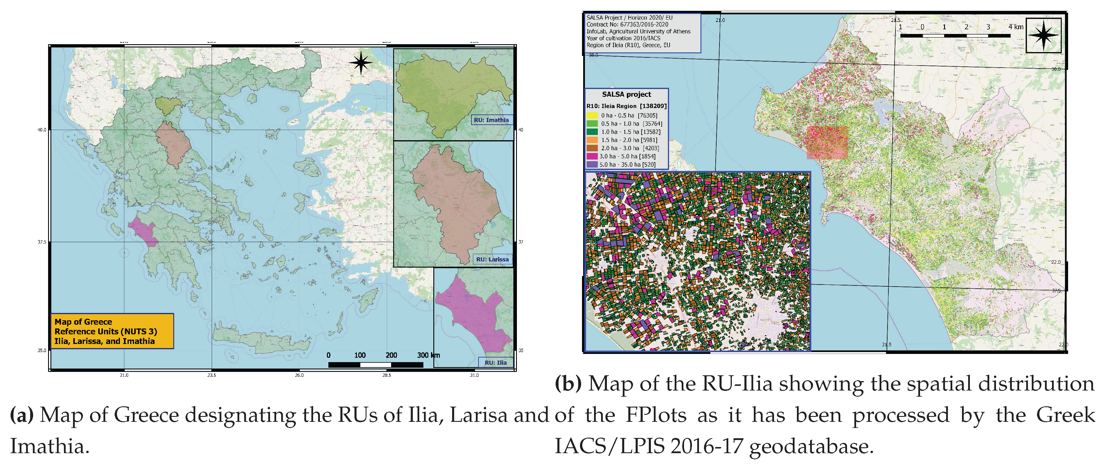
Figure 2.
Maps of RU-Larisa and RU-Imathia showing the spatial distribution of the FPlots as it has been processed by the Greek IACS/LPIS 2016-17 geodatabase.
Figure 2.
Maps of RU-Larisa and RU-Imathia showing the spatial distribution of the FPlots as it has been processed by the Greek IACS/LPIS 2016-17 geodatabase.

Figure 3.
Map of (a) RU-Ilia and (b) RU-Larisa showing the spatial distribution of field points visited for crop types identification.
Figure 3.
Map of (a) RU-Ilia and (b) RU-Larisa showing the spatial distribution of field points visited for crop types identification.

Figure 4.
Map of RU-Imathia of Greece showing the spatial distribution of field points visited for crop types identification.
Figure 4.
Map of RU-Imathia of Greece showing the spatial distribution of field points visited for crop types identification.
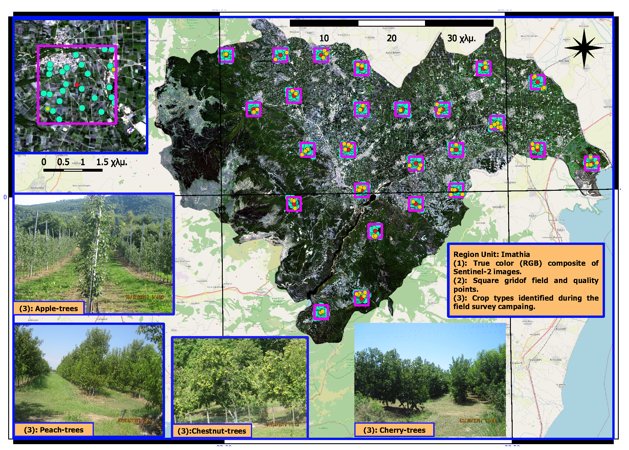
Figure 5.
Field points intersection with segments (agricultural plots) generated during the image segmentation stage [39].
Figure 5.
Field points intersection with segments (agricultural plots) generated during the image segmentation stage [39].
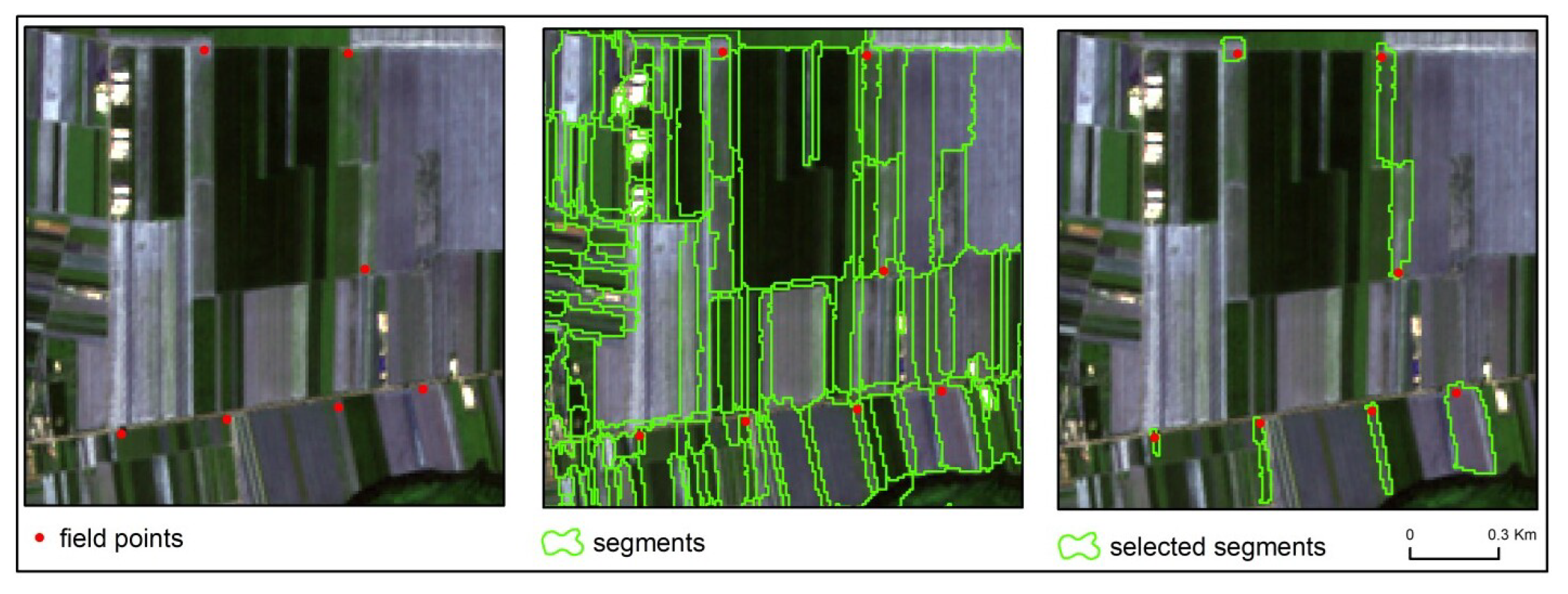
Figure 6.
Intersection of olive segments (a) and vegetables (legumes) segments (b) derived from the RS approach (Cultivation period 2017-18, RF classifier) with FPlots derived from IACS/LPIS 2016-17 geodatabase.
Figure 6.
Intersection of olive segments (a) and vegetables (legumes) segments (b) derived from the RS approach (Cultivation period 2017-18, RF classifier) with FPlots derived from IACS/LPIS 2016-17 geodatabase.
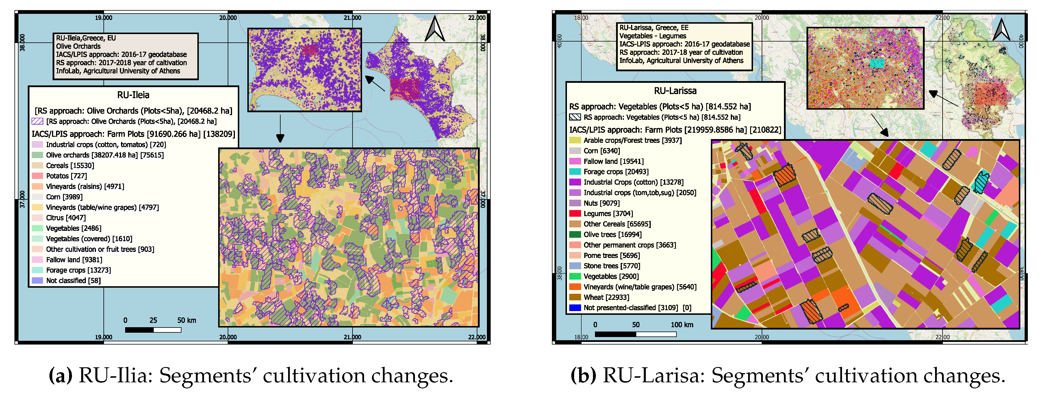
Figure 7.
(a) Intersection of peaches segments derived from RS approach (Cultivation period 2017-18, RF classifier) with FPlots derived from IACS/LPIS 2016-17 geodatabase. (b) Crops’ map derived from the RS approach (Cultivation period 2017-18, RF classifier) highlighting the small agricultural plots (segments<5 ha).
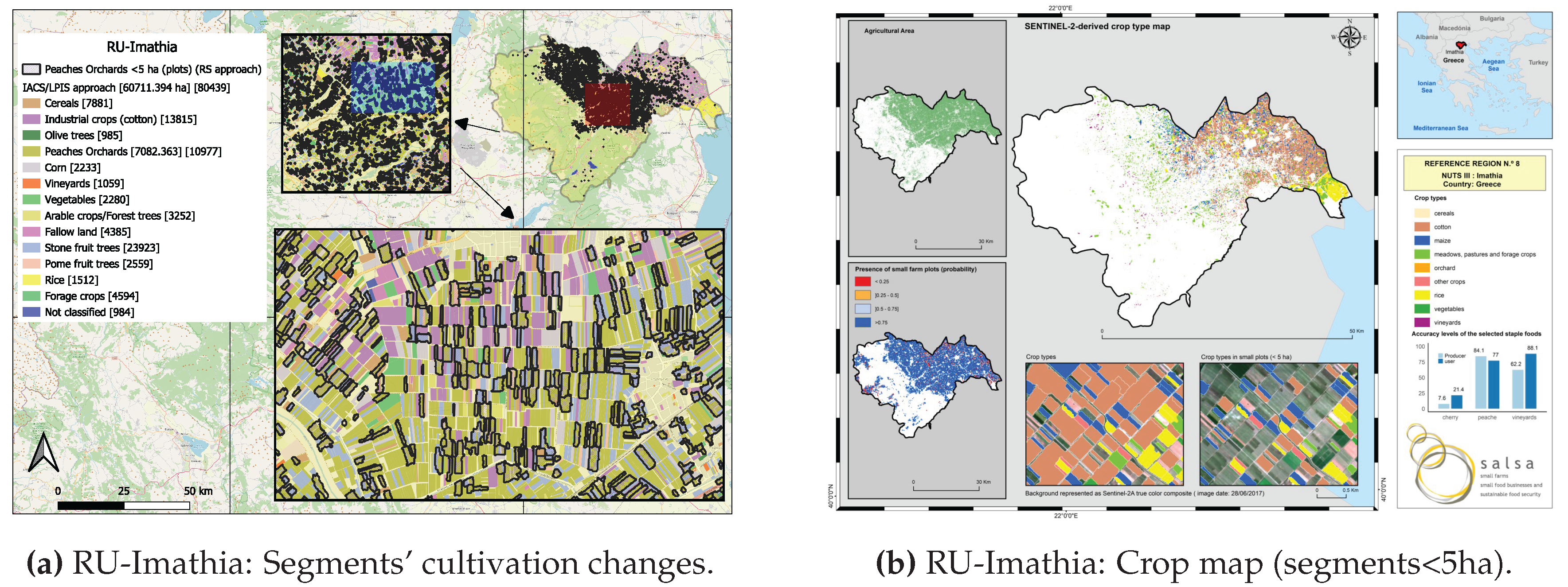
Table 1.
Number of records per country per LUCAS field-survey. In-situ (direct observations), In-situ Photo-Interpreted (not accessible points), On desk Photo-Interpreted (not in-situ) per year. * Year 2022 data is not included in the totals.
Table 1.
Number of records per country per LUCAS field-survey. In-situ (direct observations), In-situ Photo-Interpreted (not accessible points), On desk Photo-Interpreted (not in-situ) per year. * Year 2022 data is not included in the totals.
| Observations per LUCAS field-survey | |||||||
|---|---|---|---|---|---|---|---|
| Type | 2006 | 2009 | 2012 | 2015 | 2018 | 2022* | Totals |
| In-situ | 155,238 | 175,029 | 243,603 | 242,823 | 215,120 | 199,080 | 1,031,813 |
| In-situ PI | 13,163 | 59,594 | 26,669 | 25,254 | 22,894 | 147,574 | |
| On desk PI | 71,970 | 99,803 | 171,773 | ||||
| Other | 96 | 37 | 133 | ||||
| Total | 168,401 | 234,623 | 270,272 | 340,173 | 337854 | 399,648 | 1,351,293 |
| # EU MSs | 11 | 23 | 27 | 28 | 28 | 27 | |
Table 2.
Ilots classification used by the Greek IACS/LPIS 2016-17 database.
| Crop/Land Description | LPIS Code |
|---|---|
| Arable crops - Forest trees | 45.2 |
| Citrus for processing | 19, 37 |
| Corn | 3.1 |
| Fallow Land | 6 |
| Forage crops (Fodder) | 8 |
| Industrial crops(cotton) | 12 |
| Industrial crops(tomato, tobacco, sugar-beats) | 18, 17, 10 |
| Legumes (Pulses) | 11 |
| Nuts | 21 |
| Olive groves | 15 |
| Other cereals (barley, oats, rye) | 2 |
| Pears & peaches for processing | 20.1, 20.2 |
| Pome fruit trees | 67 |
| Potatoes | 24 |
| Rice | 7 |
| Stone fruit trees | 66 |
| Vegetables | 38 |
| Vegetables(covered) | 39 |
| Vineyards(raisins) | 28.1 |
| Vineyards(table/wine grapes) | 36.2, 36.3 |
| Wheat | 1 |
Table 3.
Distribution of the number of FPlots and their total UAA (ha) covered per area class and reference RU (Greek IACS/LPIS 2016-17 geodatabase).
Table 3.
Distribution of the number of FPlots and their total UAA (ha) covered per area class and reference RU (Greek IACS/LPIS 2016-17 geodatabase).
| RU-Ilia | RU-Larisa | RU-Imathia | ||||
|---|---|---|---|---|---|---|
| Classes(ha) | UAA(ha) | #FPlots | UAA(ha) | #FPlots | UAA (ha) | #FPlots |
| 19,719.0278 | 76,305 | 23,298.9013 | 87,526 | 11,579.9082 | 37,882 | |
| 25,055.3707 | 35,764 | 37,905.2561 | 51,970 | 18,598.5394 | 26,032 | |
| 16,176.6347 | 13,582 | 32,310.3043 | 26,515 | 10,933.4992 | 9,047 | |
| 10,243.1940 | 59,810 | 26,952.6916 | 15,434 | 10,243.1939 | 3,333 | |
| 9,980.5413 | 4,203 | 39,330.8814 | 16,208 | 6,301.7193 | 2,598 | |
| 6,822.8750 | 1,854 | 36,837.1641 | 9,789 | 4,215.2849 | 1,124 | |
| 3,692.6230 | 520 | 23,324.3297 | 3,381 | 30,178.4476 | 423 | |
| Totals | 91,690.2662 | 138,209 | 219,959.5986 | 210,822 | 69,711.3942 | 80,439 |
Table 4.
Distribution of the number of Farms, the number of FPlots, and the UAA (ha) covered per reference RU and per type of farm (SFs ( ha), and Large Farms ( ha)) (Greek IACS/LPIS 2016-17 geodatabase). The values in parentheses indicate the % of change in the corresponding value reported by the Official National Statistics of Greece.
| Type of Farms | ||||
|---|---|---|---|---|
| Region | Feature | SF | LF | Totals |
| RU-Ilia | #Farms | 20,454.0 (-13.72) | 5,245.0 (16.69) | 25,699.0 (-8.88) |
| #FPlots | 77,483.0 | 60,726.0 | 138,209.0 | |
| UAA(ha) | 38,478.3 (3.66) | 53,212.0 (11.86) | 91,690.3 (8.27) | |
| RU-Larisa | #Farms | 19,179.0 (51.18) | 12,799.0 (15.36) | 31,978.0 (34.47) |
| #FPlots | 67,358.0 | 143,393.0 | 210,822.0 | |
| UAA(ha) | 44,116.2 (59.24) | 175,753.4 (15.08) | 219,981.6 (21.86) | |
| RU-Imathia | #Farms | 12,886.0 (46.18) | 3,062.0 (-18.38) | 15,951.0 (26.90) |
| #FPlots | 43,054.0 | 37,359.0 | 80,439.0 | |
| UAA(ha) | 24,710.5 (39.71) | 35,985.9 (26.91) | 69,711.4 (31.83) | |
Table 5.
The no of segments undertaken the quality control check and used in the classification model with the Overall Accuracy (OA) and the Kappa values obtained for each one of the three reference RUs considered.
Table 5.
The no of segments undertaken the quality control check and used in the classification model with the Overall Accuracy (OA) and the Kappa values obtained for each one of the three reference RUs considered.
| Segments for the classification | |||||
|---|---|---|---|---|---|
| Reference RU | Total | Training | Validation | OA(%) | Kappa |
| RU-Ilia | 486 | 368 | 118 | 78.3 | 0.73 |
| RU-Larisa | 514 | 373 | 141 | 86.8 | 0.77 |
| RU-Imathia | 500 | 371 | 129 | 91.4 | 0.83 |
Table 6.
The levels of Producer and User accuracy (PA, UA), the Omission and Commission Errors (OE, CE) , and the FScore (%) per crop derived from the confusion matrix produced for each one of the Greek reference RUs considered. Note that: (1) With * we denote the crop types that were classified using a more generalized crop cover. (2) With italics we indicate the key-crop types in the respective RU.
| Reference | Crop | Crop | PA | OE | UA | CE | FScore |
|---|---|---|---|---|---|---|---|
| RU | Type | Area | (%) | ||||
| RU-Ilia | Cerials | 70.8 | 29.2 | 89.2 | 10.8 | 78.9 | |
| Meadows, | 82.7 | 17.3 | 78.1 | 21.9 | 80.4 | ||
| pastures and | |||||||
| forage crops | |||||||
| Olive groves | 20,618.20 | 88.5 | 11.5 | 82.8 | 17.2 | 85.5 | |
| Oranges | 54.7 | 45.3 | 35.4 | 64.6 | 43.0 | ||
| Other orchards | 28.6 | 71.4 | 52.6 | 47.4 | 37.0 | ||
| Vegetables | 79.9 | 20.1 | 74.1 | 25.9 | 76.9 | ||
| Vineyards/Grapes | 2,289.35 | 74.6 | 25.4 | 80.3 | 19.7 | 77.3 | |
| Watermelons | 80.7 | 19.3 | 100.0 | 0.0 | 89.3 | ||
| RU-Larisa | Cereals | 99.3 | 0.7 | 90.0 | 10.0 | 94.4 | |
| Cotton plants | 78.2 | 21.8 | 92.0 | 8.0 | 84.5 | ||
| Maize | 80.0 | 20.0 | 94.2 | 5.8 | 86.5 | ||
| Meadows, | 47.6 | 52.4 | 65.0 | 35.0 | 55.0 | ||
| pastures and | |||||||
| forage crops | |||||||
| Olive groves | 18.3 | 81.7 | 32.8 | 67.2 | 23.5 | ||
| Other orchards | 75.7 | 24.3 | 64.3 | 35.7 | 69.5 | ||
| Vegetables (Pulses) | 814.552 | 58.2 | 41.8 | 98.7 | 1.3 | 73.2 | |
| Vineyards | 75.8 | 24.2 | 51.4 | 48.6 | 61.3 | ||
| RU-Imathia | Cereals | 82.8 | 17.2 | 72.7 | 27.3 | 77.4 | |
| Cherry | 7.6 | 92.4 | 21.4 | 78.6 | 11.2 | ||
| Cotton plants | 96.1 | 3.9 | 89.0 | 11.0 | 92.4 | ||
| Maize | 93.8 | 6.2 | 95.8 | 4.2 | 94.8 | ||
| Meadows, | 85.3 | 14.7 | 91.1 | 8.9 | 88.1 | ||
| pastures and | |||||||
| forage crops | |||||||
| Orchards | 99.5 | 0.5 | 95.5 | 4.5 | 97.4 | ||
| Other crops | 24.7 | 75.3 | 73.7 | 26.3 | 37.0 | ||
| Peaches | 8,782.06 | 84.1 | 15.9 | 77.0 | 23.0 | 80.4 | |
| Rice | 93.5 | 6.5 | 94.3 | 5.7 | 93.9 | ||
| Vegetables | 57.4 | 42.6 | 79.5 | 20.5 | 66.7 | ||
| Vineyards/Grapes | 62.2 | 37.8 | 88.1 | 11.9 | 72.9 |
Table 7.
For the year of cultivation 2017-18 the Table presents: (a) The unbiased crop area estimations provided by the RS approach for small size plots (< 5 ha), (b) The achieved per key-crop selected by the RS approach, (c) The yield and the production estimations for each key-crop product by the RS approach, (d) Crop area of all size plots and production estimations for each key-crop product provided by ELSTAT, (e) the contribution of the unbiased key-crop areas of the selected key-crops per RU derived by the RS approach (small size plots <5 ha) as a % of the corresponding total UAA of the same key-crop provided by the official statistics.
| Method Used | Key-Crop | FScore | Key-Crop | Yield Esti- | Key-Crop |
|---|---|---|---|---|---|
| per RU) | Type | Area | mation | Production | |
| () | () | () | |||
| RU-Ilia | |||||
| Olive groves | |||||
| RS approach | 85.5 | 20,618.20 | 1.31 | 27,009.84 (oil) | |
| ELSTAT | 40,153.00 | 8.634 | 346,673.00 (olives) | ||
| RS contribution | 51.35% | ||||
| Grapes/Vineyards | |||||
| RS approach | for VineTable/Raisins | 77.3 | 2,289.35 | 14.68 | 33,607.66 |
| ELSTAT | for VineTable/Raisins | 4,661,80 | 10.04 | 46,793.00 | |
| RS Contribution | for VineTable/Raisins | 49.11% | 71.82% | ||
| ELSTAT | Vine/Table | 2,025,40 | 12.31 | 24,925.00 (grapes) | |
| ELSTAT | Raisins | 2,636.50 | 3.90 | 10,286.00 | |
| RU-Larisa | |||||
| Vegetables(Legumes) | |||||
| RS approach | 73.2 | 814.55 | 3.13 | 2,549.54 | |
| ELSTAT | Legumes | 8,945.60 | 12,691.00 | ||
| RS Contribution | 9.11% | 20.01% | |||
| RU-Imathia | |||||
| Peaches | |||||
| RS approach | 80.4 | 8,782.06 | 29.99 | 263,373,98 | |
| ELSTAT | 14,716.10 | 14.69 | 245,539.00 | ||
| RS Contribution | 59,68% | 107.26% |
Disclaimer/Publisher’s Note: The statements, opinions and data contained in all publications are solely those of the individual author(s) and contributor(s) and not of MDPI and/or the editor(s). MDPI and/or the editor(s) disclaim responsibility for any injury to people or property resulting from any ideas, methods, instructions or products referred to in the content. |
© 2024 by the authors. Licensee MDPI, Basel, Switzerland. This article is an open access article distributed under the terms and conditions of the Creative Commons Attribution (CC BY) license (http://creativecommons.org/licenses/by/4.0/).
Copyright: This open access article is published under a Creative Commons CC BY 4.0 license, which permit the free download, distribution, and reuse, provided that the author and preprint are cited in any reuse.


