Submitted:
23 July 2025
Posted:
24 July 2025
You are already at the latest version
Abstract
Cryptocurrencies like Bitcoin can be considered commodities under the Commodity Exchange Act (CEA) and the Commodity Futures Trading Commission (CFTC) has jurisdiction over cryptocurrencies considered to be commodities, particularly in the context of futures trading. This paper presents a method for long and short term trend prediction of certain cryptocurrencies which is predicated on an application of the Fractal Market Hypothesis. This is an area of market theory where the self-affine properties of a fractal stochastic field are used to model a financial time series. After an introduction to the underlying theory and mathematical modelling, a fundamental analysis of Bitcoin and Ethereum to U.S. Dollar exchange markets is conducted. This analysis is based on a consideration that a changes in polarity of the 'Beta-to-Volatility' and the 'Lyapunov-to-Volatility' ratios to indicate an impending change to the Bitcoin/Ethereum price trend signal. This is used to recommend a long, a short or a hold trading position for which algorithms are provided (coded in Matlab) and 'back-tested'. An optimisation of these algorithms is conducted, leading to a strategy for implementing an ideal range of the key parameters for 'driving' the algorithms developed. This is based on maximising the accuracy and profitability to assure a high level of confidence. The application of the trading strategy developed through this approach is demonstrated to provide useful information to aid cryptocurrency investments and quantify the likelihood that the market will become bull or bear dominant. Under stable conditions, Machine Learning (using the 'TuringBot') is shown to provide useful estimates of future price values and/or fluctuations over small event horizons in time. This minimises any \lq trading delay' caused by filtering the data and increases returns by providing optimal trade positions within a \lq micro-trend' that is too fast for detection otherwise. In certain cases, this increase can reach ~10%. The results presented confirm that Bitcoin and Ethereum exchanges are self-affine (fractal) stochastic fields with L\'evy distributions, displaying a Hurst Exponent of ~ 0.32, a Fractal Dimension of ~ 1.68 and Levy Index of ~1.22. They also confirm that the Fractal Market Hypothesis and its indices provide a suitable market model, that generates returns on investments that outperform all Buy and Hold strategies based on more standard market indices.
Keywords:
cryptocurrencies
; fractal market hypothesis
; symbolic regression
; optimisation
; return on investments
1. Introduction
Starting with the introduction of Bitcoin (BTC) in 2009 [1], digital currencies, known as Cryptocurrencies, have dramatically increased in value and popularity. Founded on the idea of decentralisation and anonymity, they facilitate peer to peer transactions without the need for any central bank. Transactions are recorded anonymously on the Blockchain, a publicly accessible digital ledger. Verification of the transactions are completed by `Miners’, who solve complex mathematical problems requiring significant amounts of power before the record is added to the Blockchain. These `miners’ are compensated for their efforts with a `Gas Fee’ (unrelated to fuel), which is added to every crypto transaction. The price of `Gas’ can widely fluctuate as it depends on the current traffic on the Blockchain. As an example, Gas fees at night, can be a minute fraction of the cost during peak day times.
1.1. Context: Cryptocurrencies
Due to Cryptocurrencies initial perception as a facilitator of black market transactions and money laundering, their value over time, has seen wide fluctuations and speculation. However, as the concept of a decentralised financial network has developed, and it’s use expanded to include Non-Fungible Tokens (NFTs), computer games, and the Meta-Verse, Bitcoin’s price has sky rocketed with its current market cap at around Billion [2]. Recently, director of Fidelity Investments, Jurrien Trimmer predicted that a single Bitcoin would cost by the end of 2022 [3]. This has prompted the formation of the UK’s first `Decentralised Digital Economy Platform’ [4] and countries such as El Salvador adopting Crypto as legal tender to reduce it’s dependency on the U.S. Dollar [5]. More recently, the UK government has announced it’s intention to support the emerging cryptocurrency industry with stable coins recognised as a valid form of payment. This is part of wider plans to make Britain a global hub of crypto-asset technology [6]. Nvertheless, the value still remains highly susceptible to public opinion, with a recent increase over a period of 24 hours due to an American executive order supporting `responsible innovations’ within the industry [7], followed by an drop due to Elon Musk’s negative Twitter comments about China’s crackdown on Crypto services [8] (Cryptocurrency trading is currently illegal in China).
Due to these reactions through social media, the price of Bitcoin has proved hard to predict. As banks start to open cryptocurrency departments and offer crypto-based investment options, there is potential for the development of trading algorithms, that are applicable to crypto exchanges. Such algorithms must consider the characteristics of the market and provide trend analysis to guide investment decisions. Although there are many different cryptocurrencies in use, Bitcoin and Ethereum (ETH) are the most advanced, therefore providing the most extensive historical data sets from which to perform backtesting on any proposed hypothesis.
1.2. Market Models
For some time, a large body of research papers have concluded that financial investment instruments do not display Gaussian distributed returns (i.e the Normal distribution of price changes) [9,10]. The assumption that asset returns conform to normality comes from the fundamentals associated with the Efficient Market Hypothesis (EMH), a principle model, and standard tool for finance markets since the mid . This is based on an underlying statistical model known as the Random Walk Model (RWM). In turn, the RWM was originally based on Louis Bachelier’s study of French government bonds in 1900 [11]. In this case, Bachelier put aside the conventional `fundamental’ analysis, where predictions are purely based upon research and information, and attempted to determine the probability that a price would move up or down.
Using the phenomenon of Brownian motion, first theorised by Albert Einstein in 1905 [12], Bachelier proposed that market changes were independent and identically distributed variables [11] allowing the use of the `Gaussian’ distribution first derived by Carl Fredrick Gauss. Through developments based on the concepts presented by Bachelier, the EMH was a result of work primarily by Eugene Fama, where financial markets are considered to be `informationally efficient’, i.e. the price always reflects the available information [13]. Based on the RWM, the EMH also assumes independently random events characterised by a Gaussian distribution. The more efficient the market is, the more random the price changes are. This assumption of complete instantaneous information availability is however, not realistic and philosophically irrational, especially in the case where information is intentionally withheld [14]. Many critics hold the reliance on the EMH and it’s derivatives, such as the Black-Scholes model, to be the causes of the `Dot-Com’ crash of 2001 and the global economic meltdown in 2008 [15,16].
Conventional currency and commodity analytic methods include RWM and Monte Carlo simulations [17]. These however, have a number of disadvantages. For example, Monte Carlo analysis cannot give accurate results without a well defined underlying statistical distribution for the stochastic field. Attempts to define certain cryptocurrency distributions have proved inaccurate [18], showing the ineffective nature of current models and methodologies thereof. An evolution of the `Technical’ market theory has seen the adoption of the Fractal Market Hypothesis (FMH). This is a hypothesis for analysing financial markets based on the principals of Fractal Geometry. Discoveries that financial stochastic fields do not conform to Gaussian distributions, displaying skewed and heavy tailed Probability Density Functions (PDFs), can have a dramatic effect on risk management. The FMH assumes a non-Gaussian approach allowing for the consideration of time dependence and serial correlations within the time series. Under this model, one can develop market metrics capable of representing the instantaneous time evolution of the underlying cryptocurrencies non-stationary behaviour. This can be used to analyse trends.
In this paper, the FMH is used as the basis to develop market metrics which provide a change in polarity of the so called Beta-to-Volatility Ratio (BVR) and/or the Lyapunov-to-Volatility Ratio (LVR) signals. These metrics are used to indicate a change in trend of the Bitcoin to U.S. Dollar and the Ethereum to U.S. Dollar exchange rates. They are used to recommend a long or short trading position. This approach is tested using a Matlab based backtesting system for daily opening price data from February 12th 2016 to February 12th 2022 and hourly opening times from November 12th 2021 to February 12th 2022. An analysis of the exchanges as a whole is conducted to determine whether they are fractal stochastic fields and therefore consistent with the FMH. In addition, a Machine Learning (ML) approach based on Symbolic Regression (SR) is used to compliment the short term price predictions in periods of high trend stability. This is done in order to increase profitability over a given event horizon and further, to predict the actual value of prices in the very short term.
1.3. Structure of the Paper
This paper is structured as follows; Section 1 provides some context to the world of cryptocurrencies and standard market hypothesis in economics. Section 2 outlines the platforms available to trade in cryptocurrencies before presenting previous research and deriving two trend analysis metrics based on the FMH. Section 3 conducts an analysis on Ethereum and Bitcoin exchanges to determine their underlying distribution before presenting the functions and methods that are used in the analysis of individual financial time series. Section 4 considers the use of Symbolic Regression to provide short term estimates of the actual price of a cryptocurrency time series and not just its trend. However, it is the stability of the trend or otherwise that is used to assess the potential accuracy of such a prediction. Section 5 presents the analysis and results obtained during the work conducted. Section 6 discusses the implications of these results. Finally Section 7 provides conclusions on the work undertaken and recommends any future research. The paper is accompanied by an appendix that contains all of the relevant Matlab functions developed during the project so that readers have the facility to test the system for themselves and develop the work further, as required.
1.4. Original Contributions
The principal and original contributions in this paper are as follows:
- (i)
- Appraisal of principal FMH parameters in regard to the analysis for cryptocurrency time series.
- (ii)
- Application of the FMH to cryptocurrencies (specifically BVR and LVR metrics).
- (iii)
- Development and optimisation of Matlab software for computing said metrics and undertake backtesting.
- (iv)
- Optimisation of parameters for computing BVR/LVR for maximising profitability.
- (v)
- Application of Symbolic Regression for short term price prediction.
- (vi)
- Optimisation of input data for price prediction using Symbolic Regression.
2. Background and Theory
This section presents previous research on cryptocurrency markets and introduces the history of the FMH. In addition, key metrics, capable of determining the nature of the market under consideration, are addressed. The section also derives methods of assessing time series trend direction and stability under the assumption of a self-affine field displaying a Lévy distribution.
2.1. Previous Research
There has been a sizeable volume of academic work examining crypto price change characteristics and returns. Many of these efforts have been devoted to determining whether high market cap cryptocurrencies, such as BTC and ETH, exhibit long-term dependency in their price signals or their derivatives. The majority of the papers show evidence of crypto market inefficiency, allowing profitable trading opportunities. However, there is also a thread of evidence to suggest that BTC is becoming efficient as it evolves in time. In 2016 Urquhart examined daily price data from 2010 to 2016 to test for informational efficiency within BTC [19]. Using a number of tests including the Ljung and Box test, Runs test, Hurst exponent and Bartels test, long term memory was assessed. It was concluded that no efficiency was present and that the Hurst exponent showed strong indications of anti-persistence. However, towards 2013, it was observed that BTC began to show signs of maturity.
Research undertaken by Nadarajah and Chu in 2017 [20], which was based on similar data sets from 2010-16, split into two 3 year samples, employed additional tests such as the generalised spectral test and Portmanteau test. Results suggested a returns independence, in line with Urquhart’s findings. Long-term dependence of BTC returns and volatility was studied by Bariviera in 2017 using daily data from 2011-2017 [21]. Using De-trended Fluctuation Analysis (DFA) and sliding windows to determine the Hurst exponent, results were collected providing evidence that BTC returns show persistence reducing to efficiency post 2014. However, volatility displayed constant persistent behaviour up to 2017. Further work by Bariviera et al. in 2017 [22] determined that alternative time scales did not affect long term dependence. A further study into the long-range memory of BTC was conducted by Lahmiri et al. [23]. Their findings rejected the EMH, showing the existence of market memory under all the distribution assumptions using Fractional integrated GARCH frameworks.
In 2018, after a dramatically increasing market, Al-Yahyaee et al. [24] used daily data spanning from 2010 to 2017 to perform a comparison between BTC efficiency and other assets such as Foreign exchange. This was the first time Multifractal Detracted Fluctuation Analysis (MF-DFA) developed by Kantelhardt in 2002 had been used to evaluate the BTC market. Results indicated that BTC had the strongest long-term persistence and least efficiency of all markets under consideration. Alvarez-Ramirez et al. [25] tested BTC using DFA. Their results showed that BTC had periods of efficiency and inefficiency, with the later leading to anti-persistence. In the same year Jiang et al. [26] tested for long term dependence in daily data from 2010-17 using the Hurst exponent on a 14-day rolling window basis, Ljung and Box test and AVR test. These tests provided further evidence of inefficiency and therefore long term memory. Continued work in 2018 saw Zhang et al. [27] use daily data from 2013 to 2018 to test a collection of cryptocurrencies. Results were achieved using kurtosis and skew measurements coupled with autocorrelation and DFA. They showed that the BTC exchange was shifting towards an efficient market with a value of 0.5. However, similar to the work of Bariviera in 2017, Volatility displayed clear long term dependence. Later in 2018, Harold Hurst’s Re-scaled Range analysis (R/S) was used to evaluate persistence in the biggest market capitalisation cryptocurrencies by Caporale [28]. The time evolution of the Hurst exponent showed BTC to be becoming increasingly efficient and an instability in it’s persistence behaviour. They concluded that trend trading strategies could be used to generate profits above the standard indexes.
Moving on to 2019, Celeste et al. used R/S analysis and continuous wavelet transformations to assess the presence of fractal dynamics in BTC and ETH’s prices [29]. Their results showed strong evidence of market memory, with ETH presenting evidence of a growing underlying memory behaviour. In line with other works, BTC’s emerging maturity was also noted. Later in 2019, Hu et al. rejected the EMH by using a panel framework indicating the presence of cross-sectional dependence among high cap cryptocurrencies [30]. The Adaptive Market Hypothesis was tested for both BTC and ETH by Chu in 2019, where the effect of news and events on the exchanges was analysed [31]. This work used hourly data from July 2017 to September 2018, the Ljung and Box test and Kolmogorov-Simimov test, among others. He concluded that BTC and ETH showed time varying efficiency. It was also noted that the sentiment and type of news or event may not be a significant factor in determining efficiency.
In regard to more recent times, Al-Yahyaee et al. [32] studied the multi-fractal charactsristics of several cryptocurrencies using the time rolling MF-DFA approach and quantile regression. Results indicated long-term memory effects and the time varying inefficiency noted by the majority of other researchers. They concluded that high liquidity and low volatility increases efficiency and helps active traders utilise arbitrage opportunities. In the wake of the COVID-19 pandemic, Kakinaka and Umeno analysed the impact of the virus on the multi-fractal nature and efficiency of cryptocurrencies [33]. Using MF-DFA upon daily data from January 2019 to December 2020 they concluded that short term multi-fractal behaviour had increased but, in the long term, had decreased.
Finally, in 2021, David et al. used Auto-Regressive Integrated Moving Average and Auto-Regressive Fractionally Integrated Average methods as well as DFA to determine the persistence, randomness and chaoticity of BTC and other currencies [34]. The Hurst exponent, Fractal dimension and Lyapunov exponents were also used. Results showed the existence of long term dependence and persistence in BTC prices over daily data from July 2016 to March 2019.
The significant portion of this collection of work clearly points to a rejection of the EMH and the time evolution of BTC becoming more efficient. There is further evidence of long term memory effects, whereby a future price depends on some previous price, indicating that investors can predict future returns lowering market risk. Since the FMH assumes inherent memory within a stochastic price field, it is a natural conclusion that this mode be used in future works concerning cryptocurrencies.
2.2. Trading With Cryptocurrencies
Cryptocurrencies can be traded on a number of platforms, each with their own benefits. Examples, such as Coin-base and Binance, are trading services that cater purely to the crypto-markets, whilst other platforms such as Etoro also allow general stock and commodities trading. Each platform has its own fee structure for facilitating the buying and selling of currency. Coin-base charges for transactions [35], whilst other sites such as Etoro charge [36]. However, these are not the only charges when handling crypto-currencies. There is an intrinsic cost to add a transaction to the blockchain known as a `Gas Fee’ as discussed in the introduction. Heavily dependent on current blockchain traffic and the complexity of the transaction, gas prices can widely fluctuate, making trades far less cost effective. This can dramatically effect a trading strategy. In the example of Coin-base .v. Etoro, although the latter charges a higher base fee, it does not require a gas fee to be paid. Considering that the average gas fee is , highs can reach the thousands, this makes Etoro a more stable platform.
Currently, the Ethereum blockchain is transitioning to Eth 2.0, an upgrade that ushers in a new mechanism for adding transactions to the blockchain that is less power hungry, consequently reducing gas fees. Should this move be completed by the end of 2022, as predicted, it could change the preferred trading platform. Currently, Etoro is the only popular, internationally trusted platform that allows crypto-based options and derivatives. For the purpose of this publication, the Etoro model will be used where no gas fee is applied. The Return On Investment (ROIs) will be presented pre-fee and therefore as gross profit.
2.3. The Fractal Market Hypothesis
Work conducted as early as the 1960’s, proposed that commodity price change distributions were too peaked to be Gaussian. This became known as Leptokurtosis, a characteristic also observed by Mandelbrot [37,38]. This, and other works, indicate that the assumption of normally distributed price changes is inadequate with respect to the fundamental statistics of Financial Time Series (FTS). It prompted the development of the FMH. Formally introduced by Edgar Peter in his 1994 book entitled `Fractal Market Analysis: Applying Chaos Theory to Investment and Economics’ [39], the FMH was a culmination of work from the likes of Mandelbrot and Ralph Elliott. It was largely built upon the theory of Fractal Geometry, first proposed by Felix Hausdorff in 1918 [40] and later popularised by Mandelbrot in his 1982 book `The Fractal Geometry of Nature’ [41]. This field of mathematics studies how fractured objects exhibit self-similarity, a phenomenon where geometric features are preserved at any scale [42]. This property is intimately related to the properties of chaotic signals that can typically be generated through the iteration of strictly nonlinear functions, and modelling FTS as chaotic signals has found practical applications in a range of trading scenarios [43].
Now known to be an example of a stochastic self-affine field as a function of time, the self-affine properties of a financial sets were first recorded by Ralph Elliott in 1938 [44]. Unlike conventional calculus, in Fractional Calculus, the derivative of a function has an inherent memory. In this context (that is FMH signals can be modelled as fractional differential equations) the FMH provides a model for analysis of a financial signal where, importantly, the time series has memory, i.e. the price of a given currency or commodity depends on some previous price. This is a major advancement on the EMH, which implies that if a market is efficient then prediction is not possible. Noting that a FTS appears statistically the same at different scales, the assumption can be made that the PDFs of price values will appear the same over different time scales.
Many self-affine functions exist, with early examples including the `Lévy Curve’, developed by Paul Lévy in his 1938 paper `Plane or Space Curves and Surfaces Consisting of Parts Similar to the Whole’ [45]. Early FMH developments used another area of Lévy’s work, namely the Lévy Distribution. Benoit Mandelbrot observed that changes in cotton prices fit a Lévy distribution [46] with a Lévy Index () of 1.7 [38]. The Levy Index provides a measure of a distributions deviation from the norm, with the FMH assuming , where lower values of indicate longer tails and a higher peak; higher values indicating the opposite; and being the case for a Gaussian distribution. As the Lévy index falls further from 2, the probability of rare but extreme events, so called `Lévy Flights’, increases.
There are other metrics used to determine a signals fractal characteristics. Mandelbrot, using principles of Brownian motion applied to asset prices, attempted to show that when markets exhibit long-term dependence, their trend will have a tendency to continue. He went on to develop a metric capable of determining a fields persistence (trend continuation) or anti-persistence called the Hurst exponent (H). Named after Harold Edwin Hurst’s work concerning damn development on the river Nile in 1906 where he discovered that the range of high to low water levels increased by a fractional power law [47]. Essentially a measure of long-term memory, when , a time series exhibits anti-persistent behaviour (uncorrelated in time). When , a time series shows persistence (correlation). In the context of a FTS, a high H manifests itself as a price that is bias in a certain trend direction over time. This suggests that in terms of a RWM the price value deviates by a greater distance from it’s origin. Both parameters and H are related to the Fractal dimension (), which is itself a measure of a fields complexity at different scales, i.e. a measure of self-affinity [48]. These can all be determined through the Spectral Decay Coefficient () which is outlined later in this report.
Given that fractals are iterative processes relating to `Chaos Theory’, there is an implicit connection between `Chaos’ and the FMH. In this respect, another important parameter is the Lyapunov Exponent (). It characterises a systems level of chaotic behaviour, i.e. its evolution from non-chaotic to chaotic. On this basis, can be used to determine the evolution of a FTS and aid trend analysis (as discussed in this report). With these metrics (H, , and ), the analysis of irregular time series becomes relatively straightforward, within the context of the FMH.
2.3.1. Characteristic Indices
The observation that price changes in a FTS are inefficient [9] allows the introduction of a number of further indices to analyse the variability in stochastic field distributions. These act as a metric of the data’s deviation from the normal distribution and characterise the fields susceptibility to undergo Lévy flights and exhibit long term market memory. Moreover, these metrics can all be defined through linear relationships of the spectral decay coefficient, , for a self-affine stochastic fields’ power spectrum. Therefore, definitions of these indices can be reduced to the calculation of the .
The power spectrum of a self-affine signal decays according to a power law [49].
where is the spectral frequency (specifically the temporal angular frequency) and c is a real constant. Using logarithms, the above equation can be re-written as
from which the value of can be obtained by determining the gradient of a linear regression applied to the power spectral log-log plot. In computational terms, application of the least squares regression formula provides a value of when applied to the entire field. The Matlab code for calculating is shown in Appendix A.8. Using this result, the following standard algebraic formulae for the following measures can be obtained:
where H is the Hurst Exponent [50].
where is the Fractal Dimension of the signal [41].
where is the Levy Index [51]. These measures and their meanings with respect to stochastic field distributions and the relevant cryptocurrencies are discussed in Section 2.3.
A FTS commonly consists of a set of discrete values, representing the price of a currency or commodity. There is value in developing deterministic models to analyse economic systems, providing such a quantitative analysis can aid the management of risk. However, large markets are usually functions of random variables characterised by external influences which are complex and therefore difficult to define. These influences on the system are compounded due to their non-linear nature caused by feedback, a market reacting to itself, or its sensitivity to shocks under `market memory’ conditions.
For these reasons, the models are often relatively complicated. By dispensing with the efficient market view of economic systems in favour of a fractal base, an index to predict the future price trend behaviour can be developed as outlined in the following discussion. The goal is to develop a single measure capable of predicting the start of an upward (bull) or downward (bear) trend in a cryptocurrency price.
A standard model for a signal , in this case a continuous, time dependent currency price, is embodied in the equation
where ⊗ denotes the convolution integral,
In Equation (4), is the Impulse Response Function, is the Source Information Function and is the stochastic function of time - residual and additive noise [52]. An inherent problem of signal processing is the extraction of the relevant information from the `noisy’ signal when only an estimate of is possible. This remains the case with financial signal processing. However, in this case, consists of a wide density of global transactions that occur throughout time. The wide and effectively random nature of these transactions produce such a broad spectrum that they can be interpreted as `White Noise’, even if this `Noise’ represents real transactions. Under this assumption, Equation (4) can be modified to
where now represents the white noise of the `system’.
Consider a financial price signal where the system noise is in fact a valid price. Then the Signal-to-Noise Ratio can be considered to be high enough that residual noise can be ignored. Due to the human element of the transaction system, the convolution is where the feedback, or transaction history, is introduced into the model. This is a linear stationary model. However, financial signals are inherently non-stationary. Thus, a metric relating to a stationary model must be applied on a moving window basis to create an `index signal’ which represents the time evolution of the metric. This signal can then be used to indicate the instantaneous nature of the signal but not used to `predict’ the future, which is a common misconception in financial signal processing.
Under the assumptions of the fractal market displaying a Lévy distribution, the standard Fourier space signal signature, , can be defined as (using convolution theorem)
where is the noise present in the system and is the transfer function of the signal given by
The temporal form of the transfer function is obtained by taking the Inverse Fourier Transform (IFT) giving [53]
where is the Gamma function and - a metric that quantifies the self-affine characteristics of the signal - and is the Heaviside step function given by
The signal is thus given by (using the convolution theorem)
The metric is related to the Fractal Dimension (), Hurst Exponent (H) and Levy Index (), and hence, by association, measures the signals persistence or anti-persistence, i.e. whether the signal is convergent (bear market trend) or divergent (bull market trend).
The self-affine characteristics of the signal for an arbitrary scaling factor, , can be analysed as follows. Suppose we let and compute for the same convolutional transform but for function instead of . Given Equation (7), this yields
and thus, we can write,
However, because is being taken to be a stochastic function, there will be differences between the time signatures observed over different time scales but, on the basis of Eq. (8), the distribution of amplitudes will remain the same over all scales. In other words, we can consider to be statistically self-similar, a property that is compounded in the equation
This is the defining characteristic of a self-affine stochastic function and therefore shows that Equation (7) is a valid representation of a fractal signal - a self-affine stochastic field.
This equation provides a method of calculating the metric (by applying regression method to the power spectrum for as discussed earlier) over an entire data set. However, this is not useful for estimating the instantaneous self-affine characteristic of the signal over time.
Suppose we consider a small `look-back’ window of data, where , is used to compute the index on a rolling basis. In this case, the resulting time varying metric will provide an indicator of the base field’s persistence such as a currency exchange rate.
Applying this approach to Equation (7), for the case when , the convolution integral can be approximated as
where
In practice, given Equation (9), T is the windowed data length, which is a fraction of the full data complement. Defining , creates a single calculable measure when and the signal is convergent, indicating an impending decay in value of the underlying currency. When there is an indication of a rise in price.
Applying logarithms to Equation (9), we obtained the linear equation
and thus, once again, using the least squares regression algorithm, the log-log line gradient is given by the value of . Implemented in code, this is a faster computational proceedure than performing rolling convolutions, especially when the FTS consists of many data points. The Matlab function for computing is provided in Appendix A.3.
2.3.2. The Lyapunov Exponent
To develop another metric capable of indicating the time evolution of a stochastic field, other properties of a FTS can be utilised. For example, suppose we model a FTS as
where is the amplitude of the signal (the price value) for the iteration and is a small -order error. This is the basis for the RWM whether it be consistent for classical or fractional Brownian diffusion. However, self-affine stochastic fields do not exhibit Gaussian properties, being more susceptible to rare and extreme events and displaying longer distribution tails, which is indicative of a Lévy distribution. Under this model, fractal fields exhibit fractional diffusion where the error in each time step can have wide and fluctuating values.
Chaos theory is a field of applied mathematics where seemingly insignificant differences in initial conditions produce significant system outputs changes. This makes long term deterministic models and predictions impossible [54]. Fractional diffusion is in itself a chaotic iterative process where the next step is the result of some form of non-linear function.
A basic form for a chaotic iterative signal is
where is some non-linear function that depends critically on the value of a parameter or parameter set. In coupled systems, a single non-linear element will render the entire system as chaotic. These systems are Iterated Function Systems (IFS). Introduced in 1981 by John E. Hutchinson, they provide methods of constituting self-affine fractal geometries and signals [55].
In regard to Equation (10) the stability of an iterative process must be quantified. This can be done by considering the following iteration.
In this case, the error at any iteration n is a measure of the rate of separation of values between two iterations. The Lyapunov exponent () is based on modelling this error as
Formally, this exponent is the measure of the rate of separation of infinitesimally close trajectories [56]. In this context it can be used to examine how sensitive a signal is to an initial condition, i.e. how chaotic (unstable) the signal is. This is because, if the error at each iteration will increase rapidly. Similarly, if the error will undergo exponential decay as the iteration progresses. From Equation (11) it is clear (summing over ) that we can write the Lyapunov exponent in the form
In the case of a FTS, is taken to the price value .
For a cryptocurrency time series, is calculated computationally as the sum of the log changes in price. From Equation (12), it is clear that if , then the iterative process is stable, i.e. it converges. Moreover, if the process will diverge. Based on this observation, a positive value of denotes a signal with a chaotic characteristic and a negative value signifies a convergent, stable system. As values of increase, so does the rate at which the signal will converge or diverge [57]. Using this simple formula applied to a FTS assumed to be of the form of Equation (5), the Lyapunov exponent can be calculated for a small `look-back’ window of size N to once again create a metric signal that will represent a time evolution of the nature of the time series. As is merely a normalisation factor, if then and visa versa. Therefore, a change in polarity of the metric is a sign of the gradient of the time series, and thereby an indicator of the growth or decay of the currency price. The Matlab code used to implement this calculation for an input time series is presented in Appendix A.1.
2.3.3. The Lyapunov-to-Volatility Index
The accuracy of a FMH trend indicator, be it the Lyapunov or Beta indexes, relies on the size of the moving window used during the calculation. This moving window introduces a trading delay into the system directly proportional to it’s size. In the case of and , transitioning from positive to negative, or visa-versa, is an indication of a transition in price trend. This transition manifests as the metric’s graphical zero-crossings. However, this in itself, is not a measure of the stability of this trend.
The volatility, , is a measure of FTS stability. A trend indicator can be scaled using the volatility to produce not only a predictor of future trends, but also as a measure of the stability of that trend. In the case of the Lyapunov exponent, the resulting index is the Lyapunov-to-Volatility Ratio;
where the volatility is defined as
where is the price value. The Matlab function for computing the volatility is presented in Appendix A.2.
The same scaling can be applied to , i.e. , which now provides a different method, from a different theoretical base, to indicate changing price trends and their stability. These can be compared during system testing to observe any changes in accuracy or returns.
Although the LVR can now double as a stability indicator, the position of the zero-crossings, which recommend long or short positions, will depend on the accuracy of . This itself depends on the inherent `noise’ present within the FTS. A FMH model assumes stationarity, which is not the case in Lévy distributed stochastic fields. Their tendency to exhibit Lévy flights create `micro-trends’ that can have a dramatic effect on the system. This can yield errors in the exact position of the zero-crossings (buy/sell positions), especially with respect to small term trend deviations.
To mitigate this effect, a moving average filter can be applied to the FTS, , reducing the effect of the noise. This can be represented in the following continuous form;
where calculates the mean of the windowed data of length W. This method is also applied to the resulting LVR signal so that
In this case however, the windowed data is of length T, the financial index calculation period. Using the LVR, the zero-crossings are simply defined by the following Kronecker delta functions:
where t is the current position of the time series and is a small time step. Essentially, represents the end of a bear trend and the beginning of a bull trend and the opposite transition is represented by . Combined with the previous Matlab functions, this provides a method of trend prediction that can be used to analyse BTC-USD/ETH-USD FTS and recommend long or short trades. Exploration into the optimisation of the W and T parameters for a specific FTS is conducted in Section 5.1.
3. Methodology
To perform trend prediction on a FTS, a suitable model for the series must be chosen. This determines the nature of the functions used to calculate any market metrics and conduct historic backtesting. The following section presents an overall analysis of the BTC-USD and ETH-USD markets to determine a `distribution of best fit’ before outlining the code implementing the equations derived in Section 2.3, the backtesing strategy, and ML short term prediction.
3.1. Cryptocurrency - An Efficient or Fractal Market
Before any trend prediction approach can be adopted, there must be a determination of whether cryptocurrencies display efficient or fractal behaviour. To achieve this, 7 years of opening prices (00:00:00 GMT) on both the BTC-USD and ETH-USD markets were collected. For the purpose of this report, only BTC-USD will be described in detail, with the accompanying results for ETH-USD presented to readers.
Figure 1 shows the price of Bitcoin from February 12th 2016 to February 12th 2022. The data was obtained from https://www.CryptoDataDownload.com using the Gemini database for Coinbase hourly prices. The extraction of this data was achieved using a Matlab function which will be introduced in Section 3.3.2. All work prepared for this paper was conducted in Matlab and Excel.
Figure 2 displays the Probability Density Function (PDF) of BTC-USD prices. The distribution clearly does not conform to the traditional `Bell Curve’ synonymous with a Normal distribution. The standard deviation was calculated to be with a Kurtosis of indicating a Leptokurtic curve with a narrow peak. The Skew is indicating a longer tail to the right.
However, this work is concerned with the distribution of price changes between daily opening prices. In this respect, Figure 3 shows the PDF of the absolute log of BTC-USD price changes. Figure 4 displays the actual price changes. The forward difference is used to purely display price changes and logs taken to remove exponential elements within the signal.
An efficient market is considered to follow a RWM where each event is random and independent. Under this consideration, price changes should follow a Gaussian distribution. However, it is clear from Figure 3 that the peaked nature of the PDF is far more indicative of a Lévy distribution. This provides some initial evidence that BTC-USD is not an efficient market. Figure 5 depicts the log price PDF with a standard Gaussian bell curve overlaid to enforce the difference.
As outlined in Section 2, the limitations of the EMH has led to the introduction of new analytic methods. The Hurst exponent (H), resulting from Re-Scaled Range Analysis (RSRA), is a measure of a signal’s persistence or anti-persistence, i.e the likelihood that the next change will be in line or opposed to the current trend direction. would signify an independently distributed signal, indicating a classical Brownian diffusion model, whilst indicates a persistent system and indicates an anti-persistent system. Using Equation (1), the Hurst Exponent was calculated, yielding a value of , confirming that the BTC-USD exchange displays anti-persistence characteristics and does not conform to conventional Brownian motion, i.e classical diffusion.
Another measure relevant to the BTC-USD time series is the Fractal Dimension (). A measure of the self-similarity of a stochastic self-affine field, it can provide insight into the power spectrum range. With being the maximum value, any value below this () will provide a quantitative representation of the fields deviation from normality. Using Equation (3) for the case of BTC-USD, . This is further evidence that this exchange is not an efficient market.
Finally the Lévy index gives a representation of the signals variability, with recovering a Gaussian distribution of price changes and signifying a Cauchy distribution. As decreases from 2, the distribution becomes increasingly peaked. Using Equation (3) the Levy index was calculated to be , clearly indicating that the BTC-USD should be modelled as a Lévy distribution where the stochastic field is fractal in nature and susceptible to more frequent rare but extreme events called `Lévy flights’.
The power spectrum of a signal can be used to characterise any correlation present within the signal [58]. This correlation is an indicator of any long or short term memory, another characteristic of fractal self-affine fields. In the spectrum, increased intensity at lower frequencies indicate a long term market memory effect, with high intensity at higher frequencies indicating short term memory. The function to determine the correlation between two time prices for a financial time series is given by
where ↔ represents the transformation to Fourier space and the spectrum is given by
The Auto-Correlation Function (ACF) is produced by taking the IFT of the power spectrum. This provides a measure of how present price data is correlated with future prices. According to the EMH, the time series should be uncorrelated and therefore exhibit no market memory. This would visually be rendered as a flat power spectrum and a peaked ACF around the origin.
The resulting power spectrum of the absolute log price changes is displayed in Figure 6, and shows that there is increased intensity at the lower frequencies, indicating long term market memory and correlation within the data set. The corresponding filtered ACF is displayed in Figure 7 and shows that there is long term market memory introduced at days, with peaks of increasing amplitude at and days. Both of these results differ from that expected under the EMH. Therefore, evidence that the BTC-USD exchange does not conform to an efficient market view.
Finally a quick comparison between Daily and Hourly price changes provides further evidence of self-affinity. In a fractal signal, the PDFs would be invariant of scale and therefore the same. Table 1 shows a compilation of all of the results for Ethereum and Bitcoin indexes. The results are all very similar confirming that both the markets are fractal.
This body of analysis provides clear indication that the BTC-USD and ETH-USD exchanges are not efficient markets. The absolute log price changes are shown to not conform to a Gaussian distribution, with a peaked and skewed PDF observed showing that price changes are not independent. They display clear long term correlation and market memory effects as well as being subject to Lévy flights. Therefore, both cryptocurrency fields have a highly non-linear, fractal, self-affine nature and require a FMH approach.
3.2. Analysis
To determine if the LVR () and BVR () are useful metrics for recommending trading positions they must be tested on real life markets. Backtesting is a well established process, allowing traders to determine how effective a trading strategy is on historical data, thereby allowing them to assess its benefits or otherwise.
Using an evaluator function, the accuracy of the trading positions, represented by the zero crossings of the metric signal, can be quantified. Operating on the fact that when , indicating a buy position, the following price trend is predicted to be positive. The next position (sell) should, therefore, be at a higher price. This case would be seen as a valid result, however, if the sell position was indicated at a lower price, this would be considered a failure as it has resulted in a net loss. This concept can be used in reverse for when , indicating a short position and a predicted downward trend.
Applied to all trading positions in the backtesting output, a combined accuracy for the data set can be determined, quantifying how many recommended positions resulted in positive returns. The function for backtesting is presented in Appendix A.4.
For this body of work, individual time series for each year of BTC-USD/ETH-USD daily opening price data were made from 2016 to 2022, as well as time series representing individual months of hourly data from Nov-Feb 2022. This allowed a wide range of data sets to be analysed on different time scales.
The backtesting function receives parameters W, filtering window width, and T, the financial index calculation window. It also normalises the raw price data so that it can be displayed on the same scale as the resulting metric signal. Finally, the function produces a split graphic displaying the metric signal (LVR), the filtered/unfiltered price data and (left plot), and the non-normalised FTS (right plot). An example of which is displayed in Figure 8.
This example uses parameters of and . It shows 8 trades in total resulting in positive returns with a total ROI of .
Another advantage of backtesting is the freedom to perform parameter analysis to find the optimum range that provides the greatest accuracy and returns. As eluded to in Section 2.3.3, the trading delay caused by pre-filtering coupled with micro-trends can cause errors in the recommended trading positions. Therefore, logically, there will be a `sweet spot’ of parameters where the delay doesn’t heavily effect the system output and still adequately reduces the noise present in the signal.
Using the function , presented in Appendix A.5, backtesting was performed on an iterative basis, where each iteration increments the parameters W and T. The function produces two mesh representations of parameter combinations against evaluator results and returns, allowing comparison between parameters that achieve optimum accuracy and profit to determine if the two are correlated in any way. Due to possible micro-trends and over filtering, position accuracy can result in a loss, as the evaluator operates using the filtered data set, not the real time series. Figure 9 shows an example evaluator mesh for the BTC-USD 2020-21 time series, where the x and z axis’ represent the parameter combinations and the y axis represents the accuracy percentage.
3.3. Code Development
Previous studies into FMH have supplied portions of code that can be used as a base to implement the equations presented in Section 2.3 [59]. A number of modifications and additional features were added for speed and ease of use. All of these relevant functions are presented in the Appendix. The main functions discussed in this section of the paper are: , which is applied to the signal before calling the function to assess the results.
3.3.1. System Optimisation
On initial testing, the function was taking minutes to complete for a parameter sweep (W, T). This put time limitations on progress. For this reason, the first step was to increase the performance of the code.
On an initial view, the iterative functions for calculating the metric signals, such as the Lyapunov Exponent (Listing 1), were using for loops, which take a total time of , where N is the total number of iterations and is the time required to complete the operations within one loop. The total time taken is increased, due to the function residing within another loop, to , where n is the total number of iterations of the outer loop.
LISTING 1: Lyapunov Function With A for Loop
%Compute the log differences of the data.
for n=1:N-1
d(n)=log(data(n+1)/data(n));
end
d(N)=d(N-1); %Set end point value.
L=sum(d); %Return the exponent.
Using vectorisation improves the speed of the function by a factor of N, as only 1 operation is required, therefore the new total time would be . This is a significant improvement when there are multiple functions being called on an iterative basis, all using data sets of data points. At this number of values, the performance is increased by a factor of , where a is the number of functions called within the loop that required a for loop. In this case, a minute runtime was reduced to seconds. A vectorised version of the function above is shown below.
Listing 2: Vectorised Lyapunov Function
%---------------------------------------------------------
% Create a vector of the data points 1 step ahead
step_ahead_data=[data(2:end),1];
% Calculate the log of the ratio of data points.
log_dif=log(step_ahead_data./data);
% Append differences log with the final value.
log_dif(end)=log_dif(end-1);
L_Exponent=sum(log_dif); %Return the Lyapunov exponent.
Further reading of the code provided reveals the use of a proprietary moving average function. On inspection, this performed in the same fashion as the native Matlab filter function with the exception that it modified the length of the input data, choosing to discard the first n elements that do not give a `fully loaded’ filter, instead of truncating the values. This has a dramatic knock-on-effect, as now the system outputs must be re-assigned a new length, using another for loop. Therefore, using the Matlab function removes another loop and decreases the complexity, as there is no longer a need to sync the system outputs together.
This is a significant benefit as the initial method of assignment relied on an x-axis array and not an index position, meaning that the output arrays had T leading 0’s before allocating the element as the value when compared to the input data. This made comparison very complicated. These changes dramatically improved the readability and speed of the functions which allowed for faster testing and therefore a more comprehensive analysis.
3.3.2. Additional Functions
In conjunction with the improvements to the system performance, a number of additional functions were created to ease analysis and handling of the cyrpto-currency historic data set. The first of these was a function capable of creating the required FTS from 7 years of hourly historical data. For this report, individual years of daily opening time data and months of hourly opening time data were required. Creating the function, presented in Appendix (Appendix A.9), allowed the raw full historical archive data set to be used. With the time step, where 1 is equal to 1 hour, and the end date of the time series, in this case 12th Feb 2022 at 00:00:00, the function is capable of finding the first element and taking the next element separated by the time step for the in days.
The ROI function, shown in Appendix (Appendix A.6), is capable of applying the resulting long/short position indicators to the real-time data and determining the price change, be it negative or positive. The summation of individual trade returns can be compared to the initial investment, the price of the first position, allowing the total percentage return on investment to be presented to the user for comparison to other market indices and trading methods. It achieves this by receiving arrays of both data and trade positions, then indexing the unfiltered price data at said positions, calculating the difference between elements. Price changes are then appended to an array before a summation and the ratios are calculated. This function was incorporated into the backtesting system so that returns are calculated concurrently with the system metrics, also allowing a returns mesh plot to be compiled when performing optimisation. There were a number of other functions created during the course of this work; however, as they are not essential to the presentation of the results, they are not presented here.
3.4. Short Term Prediction
The methods outlined in this paper so far, attempt only to predict a future movement in a FTS and use this prediction to recommend trading positions. It makes no attempt to predict the scale of said movement. Considering the variability of volatility within cryptocurrencies, attempts of prediction at arbitrary time points would be futile. However, the underlying assumption in this fractal approach is that a `strong’ BVR or LVR amplitude signifies relatively stable market dynamic behaviour, and are therefore less likely to undergo a Lévy flight. This window of stability can be exploited to conduct short-term price predictions in the effort to assist a trader achieving an optimum trade position over a short future time horizon. Setting a threshold to define this `stable period’ will assign a certain degree of confidence to any predictions made. With this approach, the BVR signal now represents not only a trend indicator but also an opportunity for short term price prediction.
4. Time Series Modelling Using Symbolic Regression
A period of trend stability empirically states that tomorrow’s price will be similar to today’s. Thus, formulating equations to represent the data up to that point in time (i.e. within the `stable period’) would allow discretised progressions into the future for a short number of time steps. This process can continue for as long as the stability period persists on a moving window basis.
This methodology suggests the use of a non-linear trend matching algorithm. In this respect, Symbolic Regression is a method of Machine Learning (ML) that iterates combinations of mathematical expressions to find non-linear models of data sets. Randomly generated equations using primitive mathematical functions are iteratively increased in complexity until the regression error is close to 0, or terminated by user subject to a given tolerance, for a pre-defined set of historical data.
4.1. Symbolic Regression
Symbolic regression is a data-driven approach to model discovery that identifies mathematical expressions describing relationships between input and output variables. Unlike standard regression methods, symbolic regression does not require the user to assume a specific functional form. Instead, it searches over a space of potential models to find the best fit for the data [60,61]. Key aspects include:
- (i)
- Representation of Models: Models are represented as expression trees, where nodes correspond to mathematical operators (e.g., +, −, ×, ÷) and functions (e.g., sin, cos, exp, log), while leaves correspond to variables or constants.
- (ii)
- Search Space: The search space includes all possible mathematical functions, expressions and combinations thereof within a specified complexity limit.
- (iii)
- Fitness Evaluation: Fitness is based on criteria such as accuracy (e.g., mean squared error) and simplicity (e.g., number of nodes in the expression tree).
- (iv)
- Parsimony: Balancing accuracy and simplicity prevents overfitting.
The applications of this approach using a specific system - TuringBot - is discussed further detail in the following section.
4.2. Symbolic Regression using TuringBot
Symbolic Regression is based on applying biologically inspired techniques such as genetic algorithms or evolutionary strategies. These methods evolve a population of candidate transformation rules over successive generations to maximise a fitness function. By introducing mutations, crossovers, and selections, the approach can explore a vast space of mathematical configurations. This approach is particularly useful in generating non-linear function to simulate complicated time series. In this section, we consider the use of the TuringBot to implement this approach in practice.
In this work, we use the TuringBot [62], which is a symbolic regression tool for generating trend fits using non-linear equations. Based on Python’s mathematical libraries [63], the TuringBot uses simulated annealing, a probabilistic technique for approximating the global maxima and minima of a data field [64]. For this reason, we now provide a brief overview of the TuringBot system.
4.3. TuringBot
TuringBot [62] is an innovative AI-powered platform designed to streamline the process of algorithm creation and optimisation. By leveraging cutting-edge artificial intelligence, TuringBot enables users to generate, test, and refine algorithms for a variety of applications, such as data analysis, automation, and machine learning, without requiring extensive programming expertise. Its user-friendly interface and advanced capabilities make it an invaluable tool for professionals, researchers, and students seeking efficient solutions to complex computational problems. TuringBot stands out as a versatile and accessible resource in the ever-evolving landscape of artificial intelligence and technology. TuringBot.com is a symbolic regression software tool designed to automatically discover analytical formulas that best fit a given dataset. Symbolic regression differs from traditional regression techniques by not assuming a predefined model structure; instead, it searches the space of possible mathematical expressions to find the one that best explains or `fits’ the data. TuringBot was developed to make this process efficient, intuitive, and accessible, especially for those without a background in machine learning or advanced data science.
Launched in the late 2010s, TuringBot was created in response to the growing need for interpretable artificial intelligence models. While most machine learning tools rely on complex neural networks or ensemble models that are difficult to understand and verify, TuringBot emphasised simplicity, transparency, and mathematical interpretability. By combining evolutionary algorithms with equation simplification techniques, TuringBot is able to produce human-readable formulas that describe complex datasets. This makes it particularly valuable in scientific, engineering, and academic contexts, where understanding the model structure is as important as prediction accuracy. The software is available for Windows and Linux and comes with a straightforward graphical user interface, allowing users to load data, configure parameters, and generate formulas with minimal setup. TuringBot also offers command-line integration for advanced users and supports exporting results for further analysis. As of the mid-2020s, TuringBot has gained a user base across various domains, from physics and finance to biology and control systems. It continues to evolve with improvements in computational performance and integration with modern workflows. The name “TuringBot” pays homage to Alan Turing, reflecting the tool’s focus on combining algorithmic intelligence with human-understandable outputs.
In an era increasingly focused on explainable AI, TuringBot stands out as a lightweight, focused solution for data modelling grounded in classical mathematical reasoning. In this context, the system uses symbolic regression to evolve a formula that represents a simulation of the data (a time series) that is provided, subject to a Root Mean Square Error (RMSE) between the data and the formula together with other `solution information’ and `Search Options’.
In this work, we are interested in using the system to simulate a cryptocurrency time series of the types discussed earlier in the the paper. For this purpose, a range of mathematical operations and functions are available including basic operations (addition, multiplication and division), trigonometric, exponential, hyperbolic, logical, history and `other’ functions. While all such functions can be applied, their applicability is problem specific. This is an issue that needs to be `tempered’, given that a TuringBot generated function will require translation to a specific programming language. This requirement necessitates attention regarding compatibility with the mathematical libraries that are available to implement the function in a specific language and the computational time required to compute such (nonlinear) functions. There is also an issue of how many data points should be used for the evolutionary process itself. In this context, it is noted that the demo version used in the case studies provided in the work, only allows a limited number of data points to be used, i.e., quoting from the demo version (2024): `Only the first 50 lines of an input file are considered’.
4.4. Example Case Study
Figure 10 shows an example of a set of 50 BTC-USD data points from August 10th 2021 to September 5th 2021 (red) and the trend match outcome of the TuringBot ML system (blue). These results were acquired by manually entering 50 data points and running the system. Here, the equation of the line was achieved after iterations with a RMS error of and mean absolute error of .
The non-linear equation for the `best fit’ shown in Figure 10 is given by
Figure 10 shows no future predictions; it is purely a trend match for a period of relative `trend stability’. The principal point is that Eq. (15) can be used to evolve a small number of time steps into the future to estimate price fluctuation. By coupling the results of doing this with the scale of the LVR, for example, a confidence measure can be associated with the short term forecast that are obtained. This is because a large positive or negative values of the LVR reflects regions in the time series where the log-term volatility is low, thereby providing confidence the the forecast that is achieved. This is the principal associated financial time series analysis provide in the following section.
5. Bitcoin and Ethereum - Financial Time Series Analysis
With the derivation of market indexes and subsequent implementation in Matlab, an analysis of BTC and ETH FTS can be performed. Using the function, a collection of series were created for two time scales, yearly opening day prices ranging from Feb 2016 - Feb 2022, and monthly opening hour prices from Nov-Feb. A List of these series for BTC-USD is given in Table 2, the same collection was created for ETH-USD.
Using these, the analysis can be done on separate time scales, to not only determine the systems overall performance, but also whether the system can capitalise on the self-affine nature of the crypto-markets. For the purpose of the report, the BVR was used for analysis with the corresponding LVR results presented later in the paper for comparison.
5.1. Daily Backtesting and Optimsiation
The first step in the analysis was to not only find the optimum parameter combinations for highest accuracy and profit, but to define a rule for selecting these parameters from a set range. Starting by running the optimisation function for the BTCUSD2021 time series, the range of parameter combinations that resulted in a 100% evaluator accuracy was observed in a three dimensional mesh plot. For the remainder of this section, the Filtering Window Width and Financial Calculation Window will be referred to as W and T respectively. Figure 11 shows the resulting mesh graphic produced by the backtesting system.
It displays a broad range of W, T combinations. Due to the delay caused by the filtering process, it is logical to choose low values of W. From the mesh there are W values in excess of 90 data points, which is equivalent to over 3 months of delay in the analysis. However, small values (i.e. ) may not smooth the data enough to make the system perform well. This is confirmed by the lack of a accuracy result with .
The effect of different sizes of T, however, is not yet fully clear. Backtesting for two combinations, one with a low T value and one with a high value, is presented in Figure 12 for BTCUSD2021. It shows that for the metric signal becomes a binary representation, alternating between . This gives the trader no indication of a fluctuation in leading to a trade position.
High T values result in sinusoidal fluctuations in making it hard to define periods of high stability and fast movements in trends. This is due to the assumption of stationarity within the windowed data, used to approximate the convolution integral in Equation (9), not being feasible for such a large value of T. Given that W values should minimise delay whilst providing enough filtering to reduce noise, a suitable limit for the values of T would be .
From this comparison, T values should aim to be . W values should aim to be small enough to reduce system delay whilst maintaining a smooth enough price signal for good system performance.
To further study the optimum range, the array of combinations that returned 100% accuracy () from the function can be used to generate a new mesh plot of ROIs. As presented in Figure 13, this proves that not all optimum positions result in profitable trade positions. High value combinations of generally result in a loss over the year. However, from the topology in Figure 13, it is clear that low values of result in profitable trades irrespective of W.
This provides evidence to suggest that the highest returns are achieved when a low value of T is chosen for the smallest W value, in this instance (For combinations only). To see how the returns for positions compare to non-optimum positions, i.e. combinations that produced less than 100% accuracy, a separate mesh plot was generated where all combinations are considered. This is presented in Figure 14, where yellow represents high ROIs and dark blue low (negative). For the mesh topology, this mesh provides evidence that the combinations do create high returns relative to all combinations. Interestingly, it also displays that very small W, T values create large losses and parameter sets where also create losses.
A significant discovery extracted from this mesh plot is that the highest possible returns do not occur at the optimum positions. The highest ROI from Figure 14 is selected and the surrounding peaks do rise higher. This can be interpreted as the result of micro-trends in the time series where non-optimum parameters have fortuitously recommended trades during a local peak or trough that has yet to influence the windowed data. The aim of the system is to ensure accuracy and confidence in the trading strategy, therefore, optimum evaluator parameter combinations are preferred to highest profit achieving combinations. This priority definition warrants another evaluation of the optimum positions. Figure 15 presents a different perspective of the data displayed in Figure 11 where only the 100% accuracy combination are displayed on a two dimensional `Top Down’ view.
Figure 15 Identifies a small grid at the bottom left hand corner where W values are within the lowest range and T values are . Knowing that this grid achieves the highest ROIs as shown in Figure 14, it is therefore, preliminarily proposed that this `Grid of Choice’ (GOC) represents the best range of to be chosen from. To provide more evidence of this theory, the same approach was taken for the other yearly time series of BTC-USD. Each year displayed the same properties lending weight to the GOC theory and evidencing that the assumption of a fractal stochastic field is constant throughout the data. Figure 16 shows the resulting `Top Down’ optimum parameter mesh (left) and the ROI mesh (right) for BTC-USD 2020-21. It shows results consistent with that of BTC-USD 2021-22. The ridge of high (yellow) returns visible in Figure 16 are in some cases higher than the returns achieved under . However, most of these parameter combinations violate the required conditions, in this case and high W values. This could be attributed to the fact that in 2020 BTC-USD had an almost constant upward trend.
With optimum parameters for 2021-22 (), backtesting was performed. Figure 17 shows the graphical output from the function with, in green, in blue, the filtered data in red and raw price signal in black. The same color format will be used for all backtesting outputs in this report. It displays the 7 trades, resulting in a return in a year when Bitcoin’s value against the dollar widely fluctuated and lost value overall.
The nature of the trading delay is clear, with the filtered data (red) lagging behind the raw price data (black). The signal shows that there are periods of general trend stability in both bear and bull directions. By inspection, it can be seen that although some trade indications occur in the trough of the filtered data, when applied to the raw signal, the difference between the two price signals results in an overall loss for that transaction. This is a result of the micro trends Bitcoin displays coupled with the trading delay and inherent volatility.
The backtesting was completed on the same basis for the rest of the BTC-USD financial time series as well as ETH-USD. Results are displayed in Table 3. From these results, it is not always possible to achieve 100% accuracy. However, this does not lead to a loss for the year. It should be noted that during the analysis of ETH-USD data, the correlation between optimum parameters and high returns, including the GOC, was observed to provide further evidence in favour of the parameter selection theory.
5.2. Hourly Backtesting and Optimisation
Given that the BTC-USD market has been shown to be a self-affine fractal signal exhibiting scale invariance, backtesting over a different scale, in this case hourly prices, should return similar results. However, as can be seen from Table 2 the monthly time series have double the number of data points. For this reason, the field is expected to have a higher level of detail and therefore noise. To inspect this, Figure 18 shows a 20 day extraction from the Jan-Feb 2022 time series. The high volatility and wild price fluctuations are more prevalent than for the daily data, with micro-trends occurring faster with bigger relative movements.
Due to the increased noise content, a higher level of filtering was expected to maintain an acceptable level of accuracy and therefore confidence in the recommended trade positions. This results in a GOC where T levels remain consistent but W values rise significantly.
As with the daily time series, the first step is to run the function for the BTCUSD Jan-Feb 2022 field. Figure 19 shows the resulting mesh plot for all parameter combinations. Compared to the daily data, the general topology is far lower and as excepted, 100% accuracy is achieved with much higher values of W, in this case . T values remain consistently low, an expected result due to the self-affinity of the underlying price signal.
Taking a further look at the `Top Down’ view of the optimisation mesh plot in Figure 20, few accurate combinations of parameters exist. However, even with the sparsity of the results, there is still a clear grid containing the small range of W values for low T values. This is consistent with the expected findings. Producing the mesh plot for parameter returns, Figure 21, confirms that the GOC remains a source of strong returns.
Analysing the mesh plot of ROIs, the topology suggests an ideal location for parameters with returns around being a peak surrounded by low and negative results. This lends further evidence that the GOC is a valid theory. An interesting outcome is the plateau of high returns for high T values, irrespective of what filtering is applied. Many of these combinations are invalid due to or , the ideal range of filtering for this data. An explanation for this could be that for high values of T, the metric signal becomes heavily sinusoidal, containing low frequencies. This could result in low numbers of trades operating at heavily delayed trade positions that are fortuitously executed. Other anomalous peaks in returns surrounding the origin also violate the rule. Such small filtering sizes increases the expected number of trades to high and infeasible values, due to the fees synonymous with trading cryptocurrencies. A comparison of these two invalid combinations is shown in Figure 22. In the backtest, a 0% accuracy still gives a positive return, confirming the anomalous nature of these combinations.
The sharp and focused nature of the peak suggests that the effect of micro trends in the hourly time series is greater. Returns are reduced rapidly at small deviations from optimum combinations. The backtesting output for is shown in Figure 23. 9 trades are executed resulting in a ROI. The increased volatility in the time series is reflected in the corresponding volatility in .
When applied to the other monthly time series, an interesting observation is the increase of filtering required as the fields evolve in time, suggesting that both BTC and ETH are entering a phase of high volatility. Table 4 displays the results for each monthly financial time series used in backtesting.
5.3. Analysis Using LVR
The backtests performed in previous sections were repeated for yearly financial time series using the LVR to observe any changes in results, The equivalent graphical LVR output for BTCUSD2021 is displayed in Figure 24. Results were consistent with the BVR metric, confirming that both ratios are valid for trend analysis. The LVR produced a metric signal with a greater amplitude than which provides more flexibility to change the conditions on which the trading positions are recommended. Currently trades are considered viable only when crosses the axis. However, if the signal was re-programmed to produce a delta peak when the signal reaches a certain threshold, say , this could reduce trading delay. A full set of ROI results for all BTC and ETH time series is presented in Table 5.
5.4. Returns On Investment - Pre-Prediction
A full comparison of and returns compared to the standard `Buy and Hold’ strategy (B&H), where the price change over the whole time series is taken, is shown in Table 6.
It shows that the proposed system outperforms B&H for every financial time series under consideration, both for BTC and ETH coins, with the exception of BTCUSD 2016-17 LVR. In bear dominant years of high market loss, such as BTC 2018-19, the system was capable of producing a positive return. In other cases, where the year saw high overall gains, the system was able to improve further.
These returns are high when compared to other stock market indexes, with average returns considered to be , including; S & P Commodity index returning an average between 2009 and 2019, and the S & P 500 an average of between 2005 and 2019. Overall, returns for the hourly data sets also proved to beat the B&H strategy.

Table 7.
Percentage return on investment of BTC-USD and ETH-USD for hourly financial time series using both LVR and BVR indicators compared to Buy & Hold strategy (B&H).
Table 7.
Percentage return on investment of BTC-USD and ETH-USD for hourly financial time series using both LVR and BVR indicators compared to Buy & Hold strategy (B&H).
| Year | BTC-USD | ETH-USD | ||||
|---|---|---|---|---|---|---|
| ROI - | ROI - | B&H (%) | ROI - | ROI - | B&H (%) | |
| Nov-Dec | 16.4 | 11.8 | -23.8 | 27.5 | 27.2 | -13.5 |
| Dec-Jan | 16.7 | 20 | -13.4 | 12.8 | 15.5 | -20.3 |
| Jan-Feb | 29.7 | 31.1 | -0.78 | 47.8 | 51.1 | -9.4 |
5.5. Short Term Price Prediction Using Machine Learning
As discussed in Section 3.4, periods of high trend stability, indicated by a `strong’ BVR amplitude, signify the opportunity for short term prediction using Symbolic Regression (SR). As this period continues, non-linear formulas can be re-generated every day based on historical opening prices on a rolling window basis. Once generated for a time point , the formula can be evolved for short term future time horizons , , ,... where n is the total number of data points used to create the formula. The hypothesis is that data points within the stable trend period can be used to generate non-linear formulas capable of guiding a trader to the optimum position execution, with the prices preceding the period being volatile and therefore detrimental to the SR algorithm.
Applying this to the BTCUSD2021 time series, a high BVR period can be defined as or and designated . The BVR signal reaches this threshold on the 21st of August, indicating the ability to utilise SR. Advancing forward 34 days to September 10th, still within the , the TuringBot is used to generate a trend formula using the previous 34 days opening prices (). The resulting solution is
Using this equation, data points , , , ... can estimate price fluctuations over a short time horizon. Figure 25 shows the actual BTC-USD price data from Aug 21st to Sep 20th in black, the trend `fit’ for historical data up to Sep 10th, shown in blue, and then future estimated prices for + 5 days to Sep 15th in red and +10 to Sep 20th in green. Each price estimation figure will use the same format.
Observing the SR output graph, it is clear that the prediction provides no useful guidance. It doesn’t predict the large drop in price on day 36, nor the increase in the preceding days. An optimal profit would have been achieved by exiting the long position on day 36 at . However, the prediction estimates , a price gap of nearly . During the backtesting for this data set, a short position was recommended on September 20th at . Using Figure 25 as a reference, no increased profit would have been created. On September 16th () drops below and ceases. This proves that no additional profit could have been made by the ML system. Formulas were generated for days 30-34, to see if an earlier prediction would have yielded better results. In every case, the estimated future prices gave no accurate guidance and failed to optimise the sell position. Figure 26 contains prediction plots for (top) and (bottom). The latter of which shows widely fluctuating prices and provides no confidence in it’s accuracy.
As a test, Figure 27 shows the non-linear formula generated at September 7th (Day 34) using the preceding 31 data points within and an additional 3 points from before the stable period began (i.e. ). This test goes against the ML hypothesis.
This output does provide credible guidance, indicating an exit of the long position on September 10th (Day 37) for . Compared to the zero-crossing recommendation on September 20th, this new trade position increased profit by or , a significant increase in profit. To examine this further, Figure 28 shows a formula generated for August 2nd to September 7th, now using 20 data points from outside the ().
This result is based on using the following equation:
giving a very accurate prediction. It correctly estimates the short price rise before the sharp fall. An indicated exit on September 11th at increases profit by or . The interesting observation here is that more precise price estimations came from extending the `look-back’ window beyond the . Due to the manual nature of the TuringBot, this process was only completed for the BTCUSD2021 time series and not for all time series.
6. Discussion
The analysis of both the cryptocurrencies considered in this research, has shown clear indications of non-normality (i.e non-Gaussian behaviour). This is a defining characteristic of a fractal stochastic field. The peaked and broader side bands of the PDF for these financial signals deviate from a Gaussian PDF model, violating a core principle of the EMH. Disregarding the assumption of an efficient cryptocurrency market allows various indicators to be utilised to determine the financial fields nature. All these indicators were calculated as linear functions associated with spectral decay of the signal which was obtained through linear regression of the log power spectral plot. However, this method can lead to inaccuracies due to the erratic nature of the log power spectrum. As seen in Figure 29, the gradient of the log-log regression line could have a range of values.
In order to obtain an accurate value of , precise calculations of the spectrum and optimum region for fitting the regression line are required, which in most cases is not available [65]. As all of the indicators considered are linearly related, more precise methods of calculating their values are available, such as the `Higuchi method’ for determination of and the algorithms for computing the Hurst exponent [66,67]. However, in the case of crypto-markets, the collection of indicators used showed such high deviations from normality that their inaccuracy would have made no difference to the conclusions in association with the application of a self-affine field model.
Each index showed a different aspect of deviation. The Hurst exponent (H) showed a level of anti-persistence not consistent with RWMs. The Levy index () indicated a peaked PDF, indicative of a Lévy distribution, not a Gaussian distribution. The value of the fractal dimension () showed that the field has a narrower spectrum consistent with a self-affine signal. The ACF showed clear signs of data correlation, long term market memory. This provided an overwhelming amount of evidence that the standard market hypothesis is not applicable and therefore the potential inaccuracy in the computation of can be ignored.
During backtesting and optimisation, a range of ideal values for the W, T parameters was alluded to. The need to reduce trading delay, whilst minimising the noise in the signal, proved to be dependent on the time scale of the time series, with larger filtering windows being required for the more detailed hourly data fields. Financial calculations had to be undertaken over small time windows relative to the length of data being analysed, whilst staying above the limit of 2. Unlike W, T values did not increase with an increase in scaling. Observing the positions, the location of the GOC can be acquired. This is related to the smallest range of W values for which T is minimised. This GOC was consistent, through all fields of the same currency and scale, leading to the guidelines for the parameter choice as follows: W - Smallest values for which noise is sufficiently removed; T - . Although this range, for the two parameters, did not always result in the most profitable trades, the high accuracy allowed high confidence in a profitable strategy. The fluctuation in ROI for neighbouring combinations can be explained by rapid micro-trends making an `ideal’ position recommendation impossible given the level of trading delay.
Another method to help overcome the trading delay is to redefine the conditions for which the position indicator produces a Kronecker delta. Currently, positions are only recommended when either or change polarity. However, if this was altered so that the Kronecker deltas were produced when a given threshold is passed, the system would react faster to changing trends. The implications of this are that price changes opposed to the current trend direction require less impact on the filter window to produce a Kronecker delta indicator.
The only down side to this change, is the increased risk due to parabolic metric flights caused by fast trend sweeps large enough to influence BVR/LVR results into recommending buy and sell positions in quick succession. However, looking at backtesting graphical outputs, it can be seen that a reduction in trading delay occurs more frequently. This change also depends on the metric used. The LVR produces a signal with a higher amplitude, giving more flexibility to choose a threshold range. Performances for both metrics were similar, as were returns in all backtests. As the metrics are derived from a different theoretical basis, one from a fractal model and the other from a chaotic model, their similar effectiveness further proves that cryptocurrency exchanges adhere to the FMH.
The self-affine behaviour of the cypto-markets under consideration allow for different time scales to be analysed. For example, Figure 30 shows an extraction from the daily backtesting output for BTC-USD 2021-22 for Jan-Feb (left) and compares it with the same backtesting time period for hourly data.
The hourly data (right) shows a number of trades being recommended with a return over a period of overall loss in value. This is in stark contrast to the daily backtest, which showed no positions, therefore resulting in a loss. The most interesting comparison, is the opposite trade positions recommended for the last few data points, with daily data suggesting a purchase and hourly data suggesting a short market position.
The higher detail in the hourly data would be expected to produce more accurate positions. However, hourly data is particularly susceptible to micro-trends, requiring a large increase in the filtering window. This makes system outputs, based on hourly data, riskier; as evidenced from the reduced returns. Even though actual price changes over a month are less than over a year, the relative movement over the time period as a percentage is directly comparable over any scale.
Coupled with an increased number of trades per unit time, which has an effect due to the fees charged by the trading platform, the hourly trading system has it’s limitations. A combination of both strategies, whereby long term trend analysis positions are complimented by short term data, will increase the likelihood that the most profitable position can be achieved.
The application of ML to aid optimum trade executions provides price estimations that were highly inaccurate when using `look-back’ data contained within the . A range of non-linear equations, of increasing length, were created for sequential time steps within the FTS, each of which failed to predict the impending change of a trend, suggesting that increasing the window length within the has no effect on accuracy. However, accurate price estimations were produced when including a range of `unstable’ data points that proceed the window. During testing of look-back windows, that included values outside of the , it was observed that longer window lengths produce more precise results that correctly predict the magnitude and direction of the next 5-8 days within an accuracy of . For example, using a window consisting of 50 data points (), including 20 unstable values, increased the profit for a single trade by .
On re-evaluation of the approach, it becomes clear that any non-linear function based on a window of `stable’ data will only continue to display this trend when evolved forward in time. This is clearly a fundamental flaw, as, by definition, this approach will not achieve the goal of predicting a future change in trend. Extending the window beyond the creates an equation that accounts for both the low volatility trend and the high volatility movements, therefore giving a more accurate representation of the data and a better basis for future estimation. Tests on a window length of produced vastly improved results, suggesting that increasing the window length is not the primary way to improve estimations. Nevertheless, increases did improve prediction accuracy by . Thus, it can be concluded that an increase in the window length, using stable and unstable data, increases future price prediction accuracy.
Considering that the BVR and LVR are both calculated using their own rolling windows of length T, this extension should be at least T steps beyond the .
The manual nature of the TuringBot results in highly inefficient calculations. The lack of SR integration within the system is a significant flaw, if ML is to be recommended as a strategy to reduce trading delay. A proprietary SR algorithm or existing library will greatly increase usability . However, this is outside the scope of this work. Extensive manual testing of the ML method was not able to be completed over the time frame available for this work. A beneficial evolution would be an implementation in Python where large ML and evolutionary computing libraries are currently available. However, more recently, TuringBot.com has released an API for their software, allowing remote access to the SR algorithm from within the system code. This provides another approach to increasing efficiency.
During code development, using truncation to preserve data length and vectorisation to improve performance proved vital to conducting an analysis, the slow nature of the original functions making the program non-viable for continued and efficient trading. The creation of the function made the system universal, where any .csv database of financial data could be uploaded and converted into a compatible time series.
Optimisation of the code resulted in a system that could generate an output in seconds. This was a significant improvement, making its use in conjunction with a live trading system viable. This decrease in computational time allows a continuous live data stream to be used, where fast tick times of a few seconds are implementable. However, this level of data requires a marked increase in filtering or new methods of creating price data. Opening daily prices can be replaced by an average of the underlying prices of the minimum time step.
7. Conclusions: Summary, Discussion and Future Directions
The fundamental analysis of BTC and ETH crypto-markets proved to be consistent with previous research. Even though the majority of these concluded that BTC was developing into a more mature and efficient market, the analysis in this paper shows that it is still far from an efficient market. Since there is no previous research on price and trend prediction for crypto-markets using similar approaches in the available literature, no comparison can be conducted.
Analysis indicated that the data does not fit a normal distributional model. For Bitcoin, the Hurst exponent was calculated to be indicating anti-persistence and short term dependence. The Lévy Index was recorded at and a Fractal Dimension of . Moreover, long term market memory was observed from the auto-correlation functions. These results prove that cryptocurrencies are not efficient markets and a fractal model is relevant. In this context, the self-affine properties were confirmed by observing similar PDFs over scaled time series, results that are reflected in Ethereum markets as well.
7.1. Summary
Based on the principles of the FMH, two basic indicators were derived from different theoretical backgrounds, both being scaled by the volatility to produce a pair of trend analysis metrics. The success of both metric signals, when examining their zero-crossings, are an indication of a change in trend. Positive returns were found for all time series analysed even in bear dominant time periods.
Analysis of parameter sweeps, gave a basis for choosing optimum parameters values. Filtering window sizes need to be minimised to reduce trading delays whilst removing noise for accurate system outputs. For the range of filter widths (W), the width of the window (T) is be chosen to be . This rule for choosing parameters was shown to give high accuracy and returns. Short time steps create time series with high levels of noise making trend prediction less accurate and more susceptible to micro-trends causing position indications that result in a revenue loss. As a result of this, it is recommended that a combination of long and short format analysis is undertaken. This is where the short term results are used to identify the most profitable time to make a position as recommended by the associated long term analysis.
Any adoption of ML to predict future price fluctuations and thereby reduce trading delay has been shown to be highly inaccurate unless the window of data points used extends back beyond the by a minimum of T steps. Longer windows containing more data points were shown to increase accuracy. With regard to general use, the TuringBot did not provide an efficient method of implementing SR. Further improvements in the system should therefore focus on a full integration.
The analysis undertaken has shown that this approach outperforms `Buy & Hold’ strategies for all the time series considered. It also outperforms benchmark returns set by stock market indices. Given the overall performance of cryptocurrencies in the last five years, this is not surprising. However, profitable returns were observed in all bear dominant time series. Any further research should explore scale combination strategies to increase profitability. A natural evolution is the development of an integrated SR algorithm. A final area for further research may be to determine whether more cryptocurrencies are fractal in nature, and if any price correlations exist between them.
7.2. Discussion
The aim of this publication has been to provide readers with a detailed background to the algorithms that have been developed. Apart from the introductory materials given in Section 1 and Section 2, the results given in this paper are, to the best of the authors knowledge, new and original, especially in terms of their application, the numerical results presented, and more specifically, the type of data that has been investigated and the results thereof., i.e., Cryptocurrencies. In this context, an important feature of the paper is the Matlab code used in the investigation, which has been provided to allow readers to re-work the results and develop the approach further. The authors consider this to be an important component of the paper, especially for readers who would be interest to implement the algorithms in the commodities markets etc.
In this context, it is worth noting that TuringBot is just one of several emerging applications in the field of genetic programming that can be used to evolve nonlinear functions for simulating real noise. Among these are various Python-based solutions that enable the development of a fully integrated Python program, eliminating the need to rely on an external application like TuringBot. One such example is gplearn, a Python library that implements genetic programming with an Application Programming Interface inspired by and compatible with scikit-learn [68].
7.3. Future Directions
The approach considered in this work is algorithmic, in the sense that long term trends and short term price values are based on a set of quantifiable algorithms and their optimisation. In the former case, these algorithms and based on functions that compute metrics associated with the Fractal Market Hypothesis. in the latter case, the algorithms are based on a nonlinear functions that are repeatedly generated using symbolic regression. In this sense, the methods presented in this work couple conventional time series modelling with machine learning. This approach is in contrast to the use of deep learning models which have the ability to capture relationships between features in time series data, for example, and long-term dependencies in data [69]. In this context, deep learning models have the ability to improve the accuracy of the results. However, the price that is paid for this is the `volume’ of training data that is required to operate a deep learning model effectively. Thus, a specific area of future research is to undertaken a comparison between the approach considered in this paper and the use of deep time series forecasting models, using data that is initially, specific to Cryptocurrency trading and other commodities.
Author Contributions
Conceptualisation: J.B.; Methodology: J.B.; Software development: A.B.; Validation: A.B.; Formal analysis: A.B.; Investigation: A.B. The authors have read and agreed to the published version of the manuscript.
Funding
The research reported in this article was partly funded by the Science Foundation Ireland.
Institutional Review Board Statement
Not applicable.
Informed Consent Statement
Not applicable.
Data Availability Statement
The software developed to present the results given in this work was based solely on the use of Matlab and the TuringBot symbolic regression software.
Acknowledgments
The authors acknowledges the support of the Technological University Dublin, Ireland, the University of Bath and Imperial College London, UK.
Conflicts of Interest
The authors declare no conflict of interest.
Appendix A. Matlab Functions
Appendix A.1. Lyapunov
function L_Exponent = Lyapunov(data)
%---------------------------------------------------------
% Function to compute the Lyapunov Exponent 'L' for data
% length N of a time period defined by tau.
% INPUTS:
% data - Input data vector for the calculation
% OUTPUTS:
% L_Exponent - Output of Lyapunov calculation
%---------------------------------------------------------
% Create a vector of the data points 1 step ahead
step_ahead_data=[data(2:end),1];
% Calculate the log of the ratio of data points.
log_dif=log(step_ahead_data./data);
% Append differences log with the final value.
log_dif(end)=log_dif(end-1);
L_Exponent=sum(log_dif); %Return the Lyapunov exponent.
end
Appendix A.2. Volatility
function Vol=Volatility(data)
%------------------------------------------------------------
%Function to compute the Volatility for data of size N.
% INPUTS:
% data - Data for computation
% N - Length of the data
% OUTPUTS:
% Vol - Result vector for the calculation of volatility
%------------------------------------------------------------
% create a vector of the data points 1 step ahead of data
%using a dummy variable '1' for last value
step_ahead_data=[data(2:end),1];
% calculate the log of the ratio of data points
log_dif=log(step_ahead_data./data);
% append differences log with the final value to negate
%final value calculated with dummy variable
log_dif(end)=log_dif(end-1);
% Return the Volatilty
Vol=sqrt(sum(abs(log_dif).^2));
end
Appendix A.3. Beta
function beta=Beta(data,N)
%---------------------------------------------------------
% Computation of the Beta Index using the least squares
%algorithm on 'data' of length N.
% INPUTS:
% data (array) - input window of data for calculation
% N (int) - Length of Data
% OUTPUTS:
% beta - Result of beta computation
%---------------------------------------------------------
% compute logarithm of the data.
xdata=log(1:1:N);
ydata=log(data);
% Compute each term of the least squares formula
%associated with log scaling law beta*log(data)
term1=sum(ydata).*sum(xdata);
term2=sum(ydata.*xdata);
term3=sum(xdata)^2;
term4=sum(xdata.^2);
% Compute beta
beta=(term1-(N*term2))/(term3-(N*term4));
end
Appendix A.4. Backtesting
function [Result,ROI] = Backtesting(W,T,time_series,show_plot)
%---------------------------------------------------------
% FUNCTION: Back-testing procedure to compute accuracy of
% trend analysis
% INPUT PARAMETERS:
% (int) W - Size of window for pre-filtering using moving
% average of data
% (int) T - Size of window for computing financial indeces.
% (array) time_series - Array of close/opening prices to be
% used, be it hourly, daily or weekly
% (int) show_plot - Flag to show figure output or supress
% during optimisation
% OUTPUT:
% Result - Array containing all the output of the evaluator.
%----------------------------------------------------------
% Create a row vector of the time_series and normalise
data=transpose(time_series);
data=data./max(data);
% Apply a moving average filter
Fdata=movmean(data,[W-1,0]);
M=length(Fdata);
% Pre-define variables
S = zeros(1,M); V = zeros(1,M);
R = zeros(1,M); F = zeros(1,M);
ZC = zeros(1,M); G = zeros(1,M);
x = [1:1:M];
%Start moving window proceses with look-back period of W.
for m=T:M
% Window the prior data.
s=Fdata(m-T+1:m);
% Compute the Lyapunov Exponent and Volatility
%B(m) = Beta(s,T); % Beta index
S(m) = Lyapunov(s); % Lyapunov Exponent
V(m) = Volatility(s); % Volatilty
R(m) = S(m)/V(m); %Lyapunov to Volatiloty Ratio (LVR).
%%% Compute zero crossings %%%
% Compute mean LVRs (post filtering then take mean
%of prior data using look-back window T).
F(m)=mean(R(m-T+1:m));
% Evaluate zero crossings from negative to
%positive half-space
if F(m)>0 && F(m-1)<=0
ZC(m) =+ 1; %Zero-crossing given positive flag.
G(m) = Fdata(m);%Assignment for later evaluation.
end
% Evaluate zero crossings from positive
% to negative half-space
if F(m)<0 && F(m-1)>=0
ZC(m) = -1;% Zero-crossing given negative flag.
G(m) = Fdata(m);% Assignment for later evaluation.
end
end % Repeat process and update plot
% Evaluate accuracy of strategy.
Result = Evaluator(ZC(W+T-1:end),G(W+T-1:end),M-W-T-1,T);
% Calculate the return on investment
ROI=Returns(ZC(W+T:end),time_series(W+T:end));
% plot time-series and output
if show_plot == 1
figure(3); subplot(1,2,1);
plot(x,Fdata,'r-',x,F,'g-',x,ZC,'b-');
hold on, plot(data,'k-'); hold off;
subplot(1,2,2); plot(time_series);
end
end
Appendix A.5. Optimisation
function Op_Pos = Optimisation(start, size, file)
%---------------------------------------------------------
% Function for optimising the parameters of the FMH system
% INPUT PARAMTERES:
% Start (int): Start position of the optimisation window,
% must have a min size of 2 to allow
% calculations within functions called
% within function
% Size (int): Size of the filtering window
% File: The financial time series
% OUTPUTS:
% Op_Pos: List of all optimum parameters which
% give the maximum efficiency.
%---------------------------------------------------------
% ensure start has a min size of 2
if start<2
start=2;
end
% pre-define loop varibales
A = zeros(size,size);
B = zeros(size,size);
% loop starting at 2 as this is the min no.
% of points required to calculate fin indicies.
for n = start:size
for m = start:size
[Result,roi] = Backtesting(n,m,file,0);
%0 used to supress output plot
A(n,m) = Result;
B(n,m) = roi;
end
end
% Locate the position of the maximum evaluator outputs.
[row,col] = find(A==max(A,[],'all'));
Op_Pos = [row,col];
disp("Max Evaluator Value = " + A(row(end),col(end)));
% Display mesh of optimised parameters and returns.
figure(20), mesh(A,'edgecolor','k');
figure(21), mesh(B);
end
Appendix A.6. Returns
function ROI = Returns(Pos_idx,data)
%---------------------------------------------------------
% Function to calucalte the Return On Investment (ROI) of
% the system under set parameters.
% INPUTS:
% Pos_idx - Array of the indicators to buy or sell
% data - Array of the financial time series (unfiltered)
% OUTPUTS:
% ROI - Output of the return on investment
%---------------------------------------------------------
data=transpose(data);
k=1;
% if there is a buy/sell indication, store the indicator,
%its position and price
for i=1:length(Pos_idx)
if Pos_idx(i) == 1 || Pos_idx(i) == -1
tick(k,:)=[i,Pos_idx(i),data(i)];
k=k+1;
end
end
if exist('tick','var')
% pre define price change variable
price_change=zeros(1,length(tick));
% initial investment is the first buy price
initial_investment = tick(1,3);
% for all elements of the buy/sell array,
% calculate price difference of long & short positions
for i=1:size(tick,1)-1
if tick(i,2)==1
price_change(i)=tick(i+1,3)-tick(i,3);
elseif tick(i,2)==-1
price_change(i)=tick(i,3)-tick(i+1,3);
end
end
% If the final indicator is a buy, calculate
% change to final data point.
if tick(end,2) == 1
price_change(end)=(data(end)-tick(end,3));
elseif tick(end,2)==-1
price_change(end)=(tick(end,3)-data(end));
end
% calculate the overall change
Return_captial=sum(price_change);
% Calcualte the percentage change from the
% initial investment in FIAT currency.
ROI=((Return_captial+initial_investment)...
/initial_investment)-1;
else
ROI=0;
end
end
Appendix A.7. Evaluator
function Result = Evaluator(ZC,G,M,T)
%------------------------------------------------------------
% FUNCTION: Evaluates accuracy of a short time trend analysis
% indicator in terms of actual price differences.
% INPUTS:
% ZC - Array composed of zeros crossing point indicators.
% G - Array composed of the time series at zero crossings.
% M - Length of Time Series analysed
% T - Period (moving window size used for data analysis).
% OUTPUT:
% Result: combined accuracy of the sustem.
%------------------------------------------------------------
% Initiate counters.
n=1; N=1;
for m = T+1:M-T-1
if G(m)>0.0
P(n) = G(m);
n = n+1;
Q(N) = ZC(m);
N = N+1;
end
end
% Initiate counters
up_good=0; up_bad=0;
% Count the number of times that an indication of an
% upward trend led to a price increase (up_good) and
%the number of times it didn't (up_bad).
for n=1:N-2
if Q(n)>0 && P(n+1) - P(n)>0
up_good=up_good+1;
end
if Q(n)>0 && P(n+1) - P(n)<0
up_bad=up_bad+1;
end
end
%Initiate counters
down_good=0; down_bad=0;
% Count the number of times that an indication of a
% downward trend led to a price decrease (down_good)
%and the number of times it didn't (down_bad).
for n=1:N-2
if Q(n)<0 && P(n+1)-P(n)<0
down_good=down_good+1;
end
if Q(n)<0 && P(n+1)-P(n)>0
down_bad=down_bad+1;
end
end
% Provide outputs on the percentatge accuracy of
% - Successfully upward trend 'Entries_Accuracy'
% - Successfully downward trend 'Exits_Accuracy'
% - The combined accuracy of both success rates
% (the 'Combined_Accuracy').
if (double(up_good) + double(up_bad)) > 0
Entries_Accuracy = 100 * double(up_good)...
/ (double(up_good) + double(up_bad));
else
Entries_Accuracy = 0.0;
end
if (double(down_good) + double(down_bad)) > 0
Exits_Accuracy = 100 * double(down_good)...
/ (double(down_good) + double(down_bad));
else
Exits_Accuracy = 0;
end
Combined_Accuracy = ...
(Exits_Accuracy+Entries_Accuracy) / 2;
Result = Combined_Accuracy;
end
Appendix A.8. Levy Index
function output = LevyIndex(data,N)
%------------------------------------------------------------
% Function: Computation of the Levy Index (gamma) using the
% least squares algorithm for 'data' of length N.
% INPUTS:
% data - Array of input data
% N - Length of data
%
% OUTPUT:
% output - Levy index
%------------------------------------------------------------
%Compute the Amplitude Spectrum
data = (abs(fft(data))).^2;
%take log of data
xdata=log(2:1:round(N/2));
ydata=transpose(log(data(2:round(N/2))));
%Compute each term of the least squares formula associated
%with log scaling law alpha*log(data).
term1=sum(ydata).*sum(xdata);
term2=sum(ydata.*xdata);
term3=sum(xdata)^2;
term4=sum(xdata.^2);
N=round(N/2); % define N for half-space
%Compute alpha
alpha=(term1-(N*term2))/(term3-(N*term4));
%Compute Levy Index
output=-alpha;
end
Appendix A.9. Read File
function [output_price,output_timestamp] = ...
readfile(input_file, time_step, time_length, end_date)
%------------------------------------------------------------
% Function for importing the data and creating the
% finanaical time series.
% INPUTS:
% input_file: contains the historical arcive data
% time_step: contains the no. of hours between each
% data point (1 day = 24)
% time_length: total time of the series in days
% end_date: end date of the series to be created in form
% - 2022-02-12 00:00:00
% OUTPUTS:
% output_price: financial time series for use in system
%------------------------------------------------------------
% import the file
price_table = readtable(input_file,'NumHeaderLines',2);
% extract the prices and time stamp from the table of data
time_stmp = table2array(price_table(:,2));
prices = table2array(price_table(:,4));
% how many data points required
no_points = (time_length*24)+1;
total_output_points=round(no_points/time_step);
% initiate output variable
output_price=zeros(total_output_points,1);
output_timestamp=string(zeros(total_output_points,1));
% find index of the first data point
idx=find(contains(string(time_stmp),end_date));
output_price(1)=prices(idx);
k=2;
for i=(idx+time_step):time_step:(no_points+idx-time_step)
output_price(k)=prices(i);
output_timestamp(k)=time_stmp(i);
k=k+1;
end
output_price=flip(output_price);
output_timestamp=flip(output_timestamp);
References
- En.wikipedia.org. Bitcoin - Wikipedia, 2022. [Online] Available at: https://en.wikipedia.org/wiki/Bitcoin [Accessed ]. 25 April.
- Coinmarketcap.com. Bitcoin - Market Cap, 2022. [Online] Available at: https://coinmarketcap.com/currencies/bitcoin/ [Accessed ]. 25 April.
- Farooqui, J.B. Will Bitcoin hit USD 100,000 or go even higher in 2022?, 2021. [Online] Available at: https://www.proactiveinvestors.co.uk/companies/news/969323/will-bitcoin-hit-us-100-000-or-go-even-higher-in-2022-969323.html [Accessed 13th April 2022].
- Portdex. Decentralised Digital Economy Platform, 2022. [Online] Available at: https://portdex.com/ [Accessed 23rd March 2022].
- Euklidiadas, M.M. LIVING WITH BITCOIN AS A CURRENCY: THE CASE OF EL SALVADOR, 2021. [Online] Available at: https://tomorrow.city/a/el-salvador-bitcoin-legal-tender/ [Accessed 21st April 2022].
- Treasury, H. Government sets out plan to make UK a global cryptoasset technology hub, 2022. [Online] Available at: https://www.gov.uk/government/news/government-sets-out-plan-to-make-uk-a-global-cryptoasset-technology-hub [Accessed 2 May 2022].
- Bambrough, B. Leak Reveals Biden’s Crypto Plans—Sending The Price Of Bitcoin, Ethereum, BNB, Solana, Cardano, XRP, Terra’s Luna And Avalanche Higher, 2022. [Online] Available at: https://www.forbes.com/sites/billybambrough/2022/03/09/leak-reveals-bidens-crypto-plans–sending-the-price-of-bitcoin-ethereum-bnb-solana- cardano-xrp-terras-luna-and-avalanche-higher/?sh=46e0131a30f9 [Accessed 10 March 2022].
- Puterbaugh, J.; Haar, R. Bitcoin Dips Below USD40,000 Again. Here’s How Investors Should React, 2022. [Online] Available at: https://time.com/nextadvisor/investing/cryptocurrency/bitcoin-crash-continues/ [Accessed 30th April 2022].
- Mandelbrot, B.B. The Variation of Some Other Speculative Prices. The Journal of Business 1967, 40, 393–413. [Google Scholar] [CrossRef]
- Fama, E.F. The Behavior of Stock - Market Prices. The Journal of Business 1965, 38, 34–105. [Google Scholar] [CrossRef]
- Bachelier, L. Théorie de la spéculation. Annales Scientifiques de l’École Normale Supérieure 1900, 3, 21–86. [Google Scholar] [CrossRef]
- Einstein, A. The Motion of Small Particles Suspended in Liquids at Rest Required by the Molecular-Kinetic Theory of Heat. Annalen der Physik 1905, 17, 549–560. [Google Scholar] [CrossRef]
- Fama, E. Efficient Capital Markets: A Review of Theory and Empirical Work. The Journal of Finance 1970, 25, 383–417. [Google Scholar] [CrossRef]
- Depalma, A. Bre-X: From Rags to Riches, Back to Rags, 1997.
- Malkeil, B.G. The Efficient Market Hypothesis and its Critics. The Journal of Economic Perspectives 2003, 17, 59–82. [Google Scholar] [CrossRef]
- Guardian, T. The mathematical equation that caused the banks to crash, 2012. [Online] Available from: https://www.theguardian.com/science/2012/feb/12/black-scholes-equation-credit-crunch [Accessed 13 April 2022].
- Scott, F. What Monte Carlo Methods Cannot Do. Human and Ecological Risk Assessment: An International Journal 1996, 2. [Google Scholar] [CrossRef]
- Chu, J.; Nadarajah, S.; Chan, S. Statistical Analysis of the Exchange Rate of Bitcoin. PLOS ONE 2015, 10, 1–27. [Google Scholar] [CrossRef]
- Urquhart, A. The inefficiency of Bitcoin. Economics Letters 2016, 148, 80–82. [Google Scholar] [CrossRef]
- Nadarajah, S.; Chu, J. On the inefficiency of Bitcoin. Economics Letters 2017, 150, 6–9. [Google Scholar] [CrossRef]
- Bariviera, A.F. The inefficiency of Bitcoin revisited: A dynamic approach. Economics Letters 2017, 161, 1–4. [Google Scholar] [CrossRef]
- Bariviera, A.F.; Basgall, M.J.; Hasperué, W.; Naiouf, M. Some stylized facts of the Bitcoin market. Physica A: Statistical Mechanics and its Applications 2017, 484, 82–90. [Google Scholar] [CrossRef]
- Salim Lahmiri, Stelios Bekiros, A. S. Long-range memory, distributional variation and randomness of bitcoin volatility. Chaos, Solitons and Fractals 2018, 107, 43–48. [Google Scholar] [CrossRef]
- Al-Yahyaee, K.H.; Mensi, W.; Yoon, S.M. Efficiency, multifractality, and the long-memory property of the Bitcoin market: A comparative analysis with stock, currency, and gold markets. Finance Research Letters 2018, 27, 228–234. [Google Scholar] [CrossRef]
- Alvarez-Ramirez, J.; Rodriguez, E.; Ibarra-Valdez, C. Long-range correlations and asymmetry in the Bitcoin market. Physica A: Statistical Mechanics and its Applications 2018, 492, 948–955. [Google Scholar] [CrossRef]
- Jiang, Y.; Nie, H.; Ruan, W. Time-varying long-term memory in Bitcoin market. Finance Research Letters 2018, 25, 280–284. [Google Scholar] [CrossRef]
- Zhang, W.; Wang, P.; Li, X.; Shen, D. The inefficiency of cryptocurrency and its cross-correlation with Dow Jones Industrial Average. Physica A: Statistical Mechanics and its Applications 2018, 510, 658–670. [Google Scholar] [CrossRef]
- Caporale, G.M.; Gil-Alana, L.; Plastun, A. Persistence in the cryptocurrency market. Research in International Business and Finance 2018, 46, 141–148. [Google Scholar] [CrossRef]
- Celeste, V.; Corbet, S.; Gurdgiev, C. Fractal dynamics and wavelet analysis: Deep volatility and return properties of Bitcoin, Ethereum and Ripple. The Quarterly Review of Economics and Finance 2020, 76, 310–324. [Google Scholar] [CrossRef]
- Hu, Y.; Valera, H.G.A.; Oxley, L. Market efficiency of the top market-cap cryptocurrencies: Further evidence from a panel framework. Finance Research Letters 2019, 31, 138–145. [Google Scholar] [CrossRef]
- Chu, J.; Zhang, Y.; Chan, S. The adaptive market hypothesis in the high frequency cryptocurrency market. International Review of Financial Analysis 2019, 64, 221–231. [Google Scholar] [CrossRef]
- Al-Yahyaee, K.H.; Mensi, W.; Ko, H.U.; Yoon, S.M.; Kang, S.H. Why cryptocurrency markets are inefficient: The impact of liquidity and volatility. The North American Journal of Economics and Finance 2020, 52, 101168. [Google Scholar] [CrossRef]
- Kakinaka, S.; Umeno, K. Cryptocurrency market efficiency in short- and long-term horizons during COVID-19: An asymmetric multifractal analysis approach. Finance Research Letters 2021, 46, 102319. [Google Scholar] [CrossRef]
- David, S.; Inacio Jr., C.; Nunes, R.; Machado, J. Fractional and fractal processes applied to cryptocurrencies price series. Journal of Advanced Research 2021, 32, 85–98. [Google Scholar] [CrossRef] [PubMed]
- Elliott, J. Coinbase Vs. Coinbase Pro, 2021. [Online] Available at https://www.investopedia.com/coinbase-vs-coinbase-pro-5120704 [Accessed 25 April 2022].
- Crypto Fees, 2022. [Online] Available at https://www.etoro.com/trading/fees/#crypto [Accessed 25 April 2022].
- Mitchell, W.C. The making and using of index numbers; A M Kelley, 1965.
- Mandelbrot, B.B. Forecasts of future prices, unbiased markets, and martingale models. Journal of Business 1966, 39, 242–255. [Google Scholar] [CrossRef]
- Peters, E.E. Fractal Market Analysis: Applying Chaos Theory to Investment and Economics; Wiley, 1994. ISBN-10: 0471585246.
- Britannica, E. Fractal Mathermatics, 2022. [Online] Available at: https://www.britannica.com/science/fractal [Accessed 10 March 2022].
- Mandelbrot, B. The Fractal Geometry of Nature; Einaudi paperbacks, W. H. Freeman, 1983.
- Soltanifar, M. A Generalization of the Hausdorff Dimension Theorem for Deterministic Fractals. Mathematics 2021, 9. [Google Scholar] [CrossRef]
- Williams, B. Williams, B. Trading Chaos: Applying Expert Techniques to Maximise Your Profits; Wiley, 1995. [Online] Available at https://c.mql5.com/3/133/ Bill.Williams.Trading.Chaos.Applying.Expert.Techniques.To.Maximize.Your.Profits.pdf [Accessed: 17 August 2025].
- Elliott, R. The Wave Principle; Lulu, 2019.
- Lévy, P. Plane or Space Curves and Surfaces Consisting of Parts Similar to the Whole; Addison-Wesley Publishing, 1938. ISBN 0-201-58701-7.
- Lévy, P. Calcul des probabilités (gauthier-villars, paris, 1925). Théorie de l’addition des variables aléatoires 1937.
- Mandelbrot, B.B. Gaussian, Self-Affinity and Fractals; Springer Publishing, 2002. ISBN: 978-0-387-98993-8.
- Mandelbrot, B.B. How Long Is the Coast of Britain? Statistical Self-Similarity and Fractional Dimension. Science 1967, 156, 636–638. [Google Scholar] [CrossRef]
- Greis, N.P.; Greenside, H.S. Implication of a power-law power-spectrum for self-affinity. Phys. Rev. A 1991, 44, 2324–2334. [Google Scholar] [CrossRef]
- Mandelbrot, B.B. Self-Affine Fractals and Fractal Dimension. Physica Scripta 1985, 32, 257–260. [Google Scholar] [CrossRef]
- Belomestny, D. SPECTRAL ESTIMATION OF THE FRACTIONAL ORDER OF A LÉVY PROCESS. The Annals of Statistics 2010, 38, 317–351. [Google Scholar] [CrossRef]
- J M Blackledge, M.L. A Review of the Fractal Market Hypothesis for Trading and Market Price Prediction. Mathematics 2022, 10. [Google Scholar] [CrossRef]
- Wikipedia. Fouirer Transform, 2025.
- G L Baker, J.B.G. Chaotic Dynamics: An Introduction; Cambridge University Press: Cambridge, England, 1996. [Google Scholar]
- Hutchinson, J. Fractals and Self-Similarity. Indiana Univ. Math. J. 1981, 30, 713–747. [Google Scholar] [CrossRef]
- Brown, R.; Bryant, P.; Abarbanel, H. Computing the Lyapunov Spectrum of a Dynamical System From an Observed Time Series. Physical Review A 1991, 43, 2787. [Google Scholar] [CrossRef] [PubMed]
- Bryant, P.; Brown, R.; Abarbanel, H. Lyapunov Exponents From Observed Time Series. Physical Review Letters 1990, 65, 1523. [Google Scholar] [CrossRef] [PubMed]
- Blackledge, J.M. Digital Signal Processing (Second Edition); Horwood Publishing (ISBN: 1-904275-26-5), 2006. [Online] Available at: https://arrow.tudublin.ie/engschelebk/4/.
- Blackledge, J.; Kearney, D.; Lamphiere, M.; Rani, R.; Walsh, P. Econophysics and Fractional Calculus: Einstein’s Evolution Equation, the Fractal Market Hypothesis, Trend Analysis and Future Price Prediction. Mathematics 2019, 7. [Google Scholar] [CrossRef]
- R Storn, K.P. Differential Evolution – A Simple and Efficient Heuristic for Global Optimisation over Continuous Spaces. Journal of Global Optimisation, 11, 341–359.
- M Dorigo, I.M.G. Ant Colony System: A Cooperative Learning Approach to the Traveling Salesman Problem. IEEE Transactions on Evolutionary Computation, 1, 53–66.
- TuringBot. Turing Bot Homepage, 2022. [Online] Available at: https://turingbotsoftware.com/ [Accessed 11 Match 2022].
- TuringBot. Turing Bot Documentation, 2022. [Online] Available at: https://turingbotsoftware.com/documentation.html [Accessed 11 Match 2022].
- En.wikipedia.org. Simulated Annealing - Wikipedia, 2022. [Online] Available at: https://en.wikipedia.org/wiki/Simulated annealing [Accessed 25 April 2022].
- Krakovská, H.; Krakovská, A. Fractal Dimension of Self-Affine Signals: Four Methods of Estimation, 2016.
- Higuchi, T. Approach to an irregular time series on the basis of the fractal theory. Physica D: Nonlinear Phenomena 1988, 31, 277–283. [Google Scholar] [CrossRef]
- Hurst, H.E. Long-term storage capacity of reservoirs. Transactions of the American Society of Civil Engineers 1951, 116, 770–808. [Google Scholar] [CrossRef]
- Python. gplearn: Genetic Programming in Python, with a scikit-learn inspired and compatible API. [Online] Available at https://gplearn.readthedocs.io/en/stable/ [Accessed: 6 July 2025].
- X Liu, W.W. Deep Time Series Forecasting Models: A Comprehensive Survey. Journal of Mathematics, [Accessed: 17 August 2025]. [CrossRef]
Figure 1.
Daily opening prices for BTC-USD from 12/02/2016 - 12/02/2022.
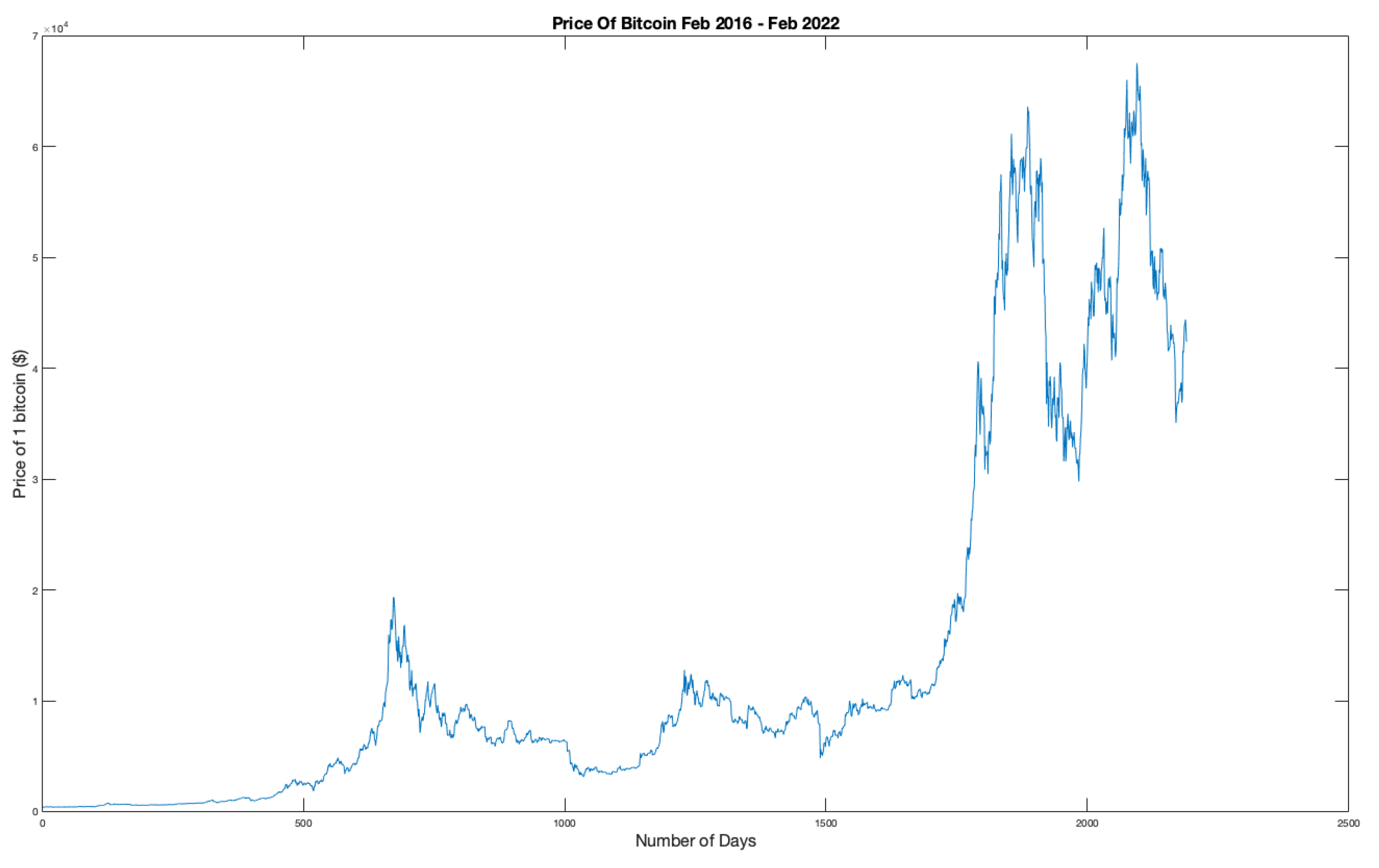
Figure 2.
Frequency histogram for BTC-USD opening prices (2016-2022).
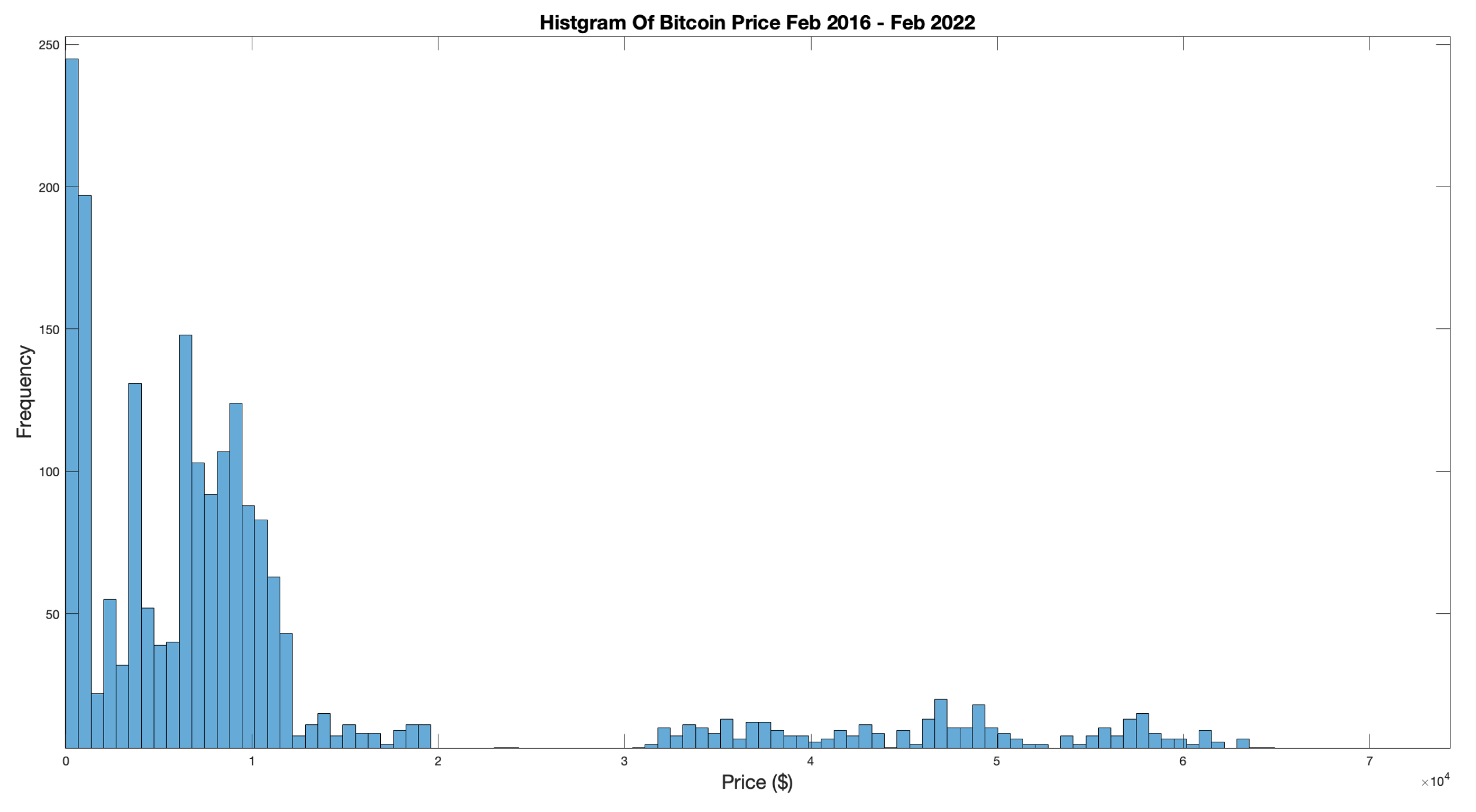
Figure 3.
Frequency histogram of log price changes for BTC-USD (2016-2022).
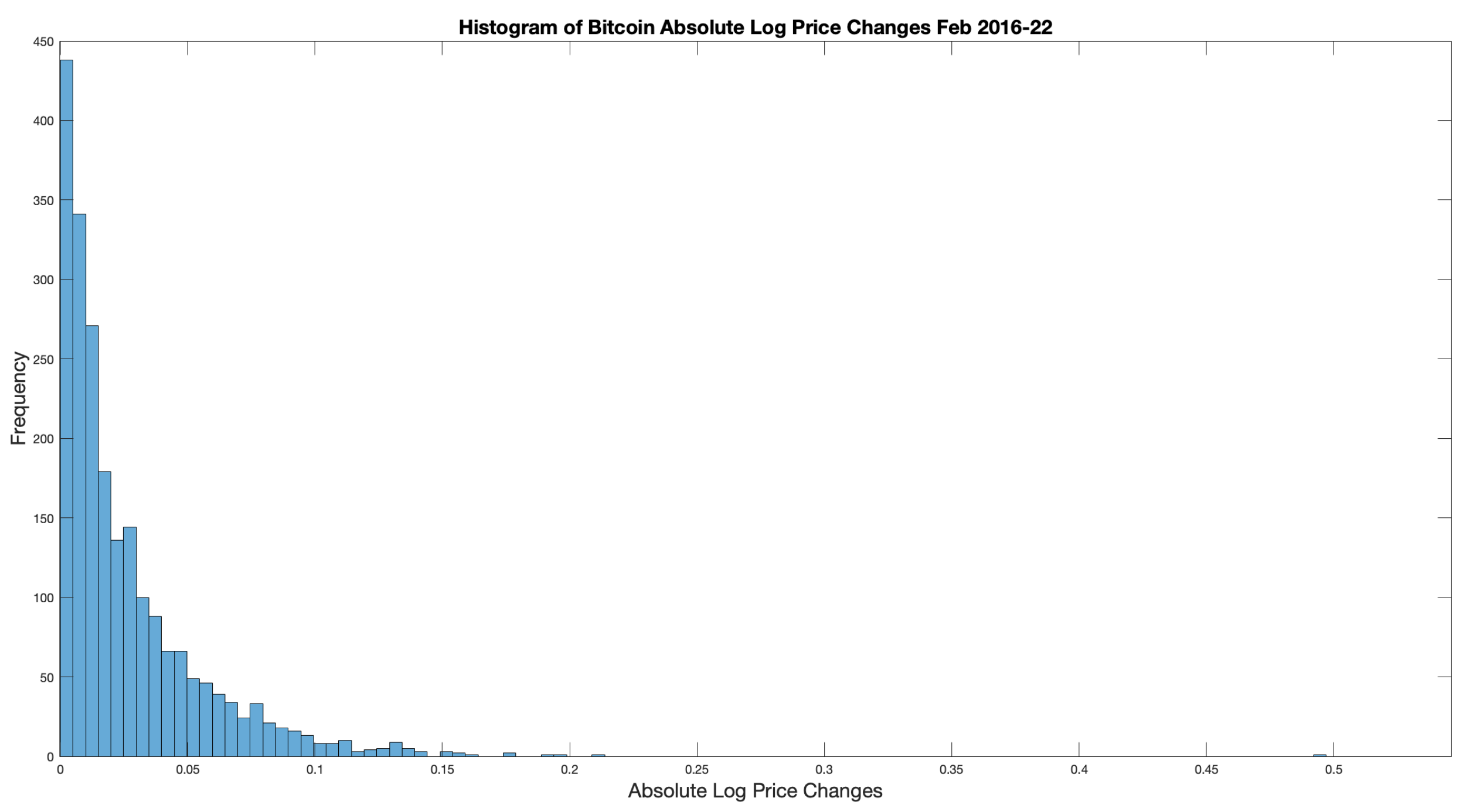
Figure 4.
Actual price changes for opening daily BTC-USD prices (2016-2022).
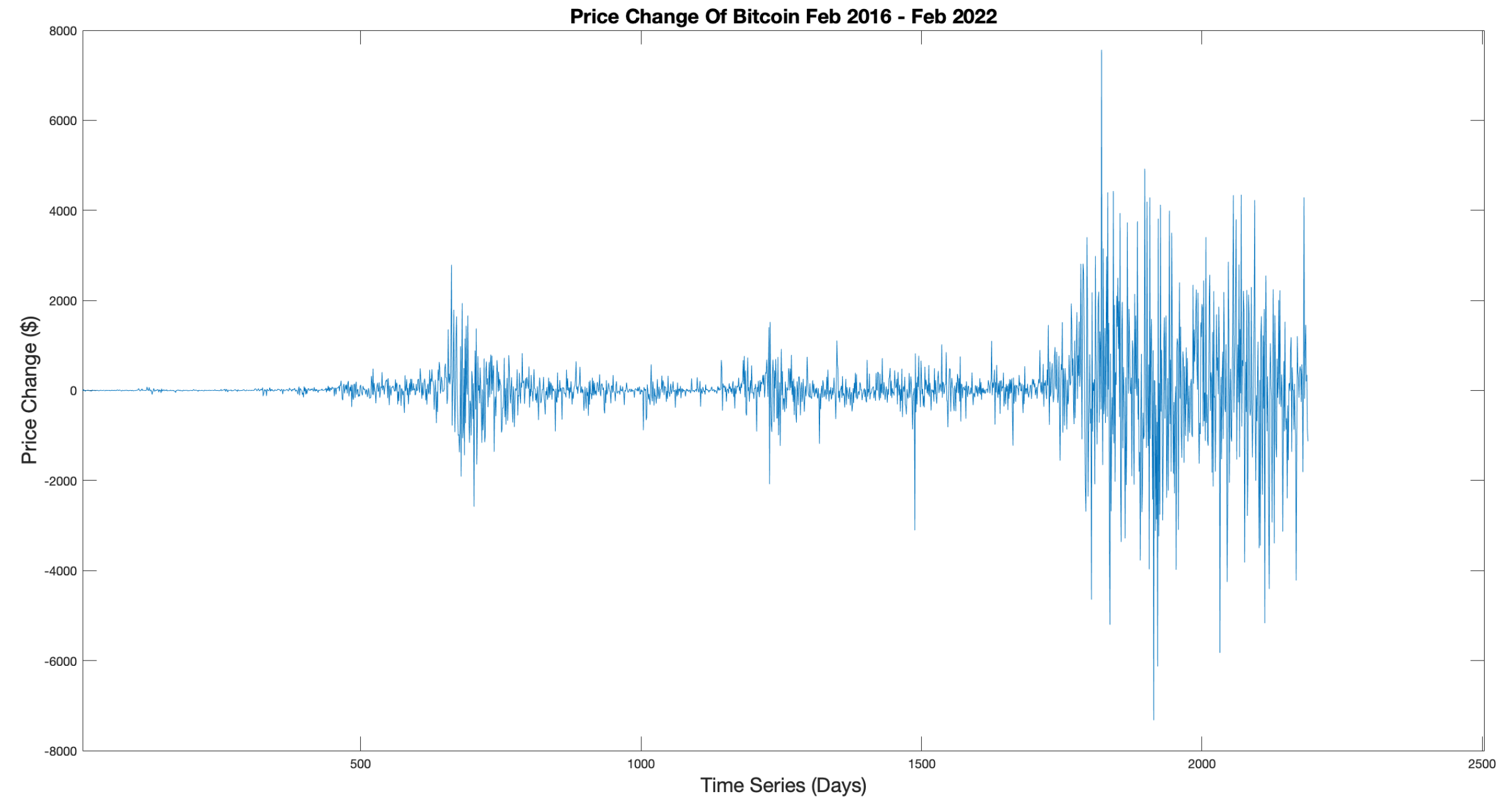
Figure 5.
Log price change probability density function for opening daily BTC-USD prices (2016-2022) Vs. standard gaussian distribution.
Figure 5.
Log price change probability density function for opening daily BTC-USD prices (2016-2022) Vs. standard gaussian distribution.
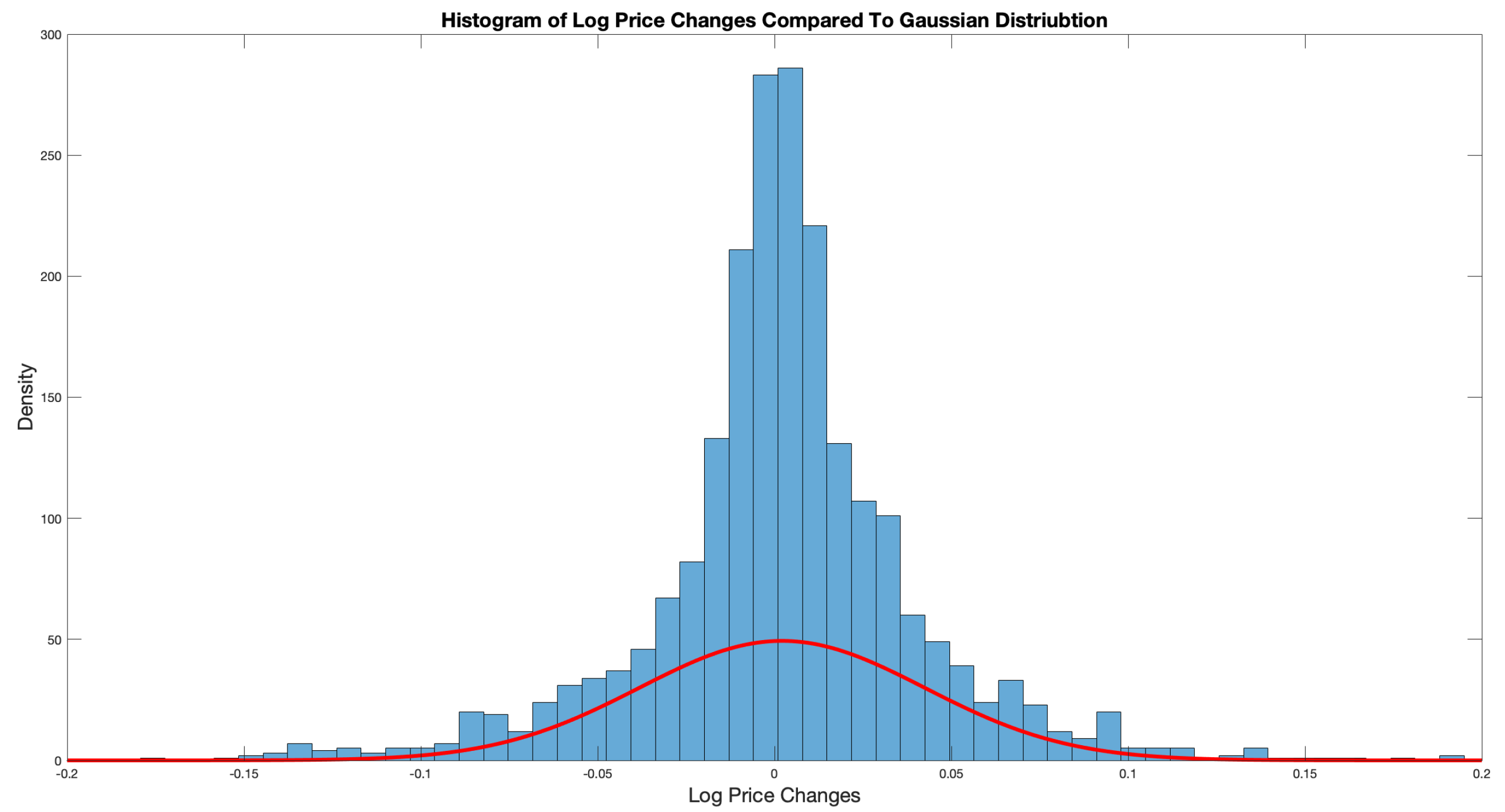
Figure 6.
Power spectrum of absolute log price change of the BTC-USD (2016-2022).
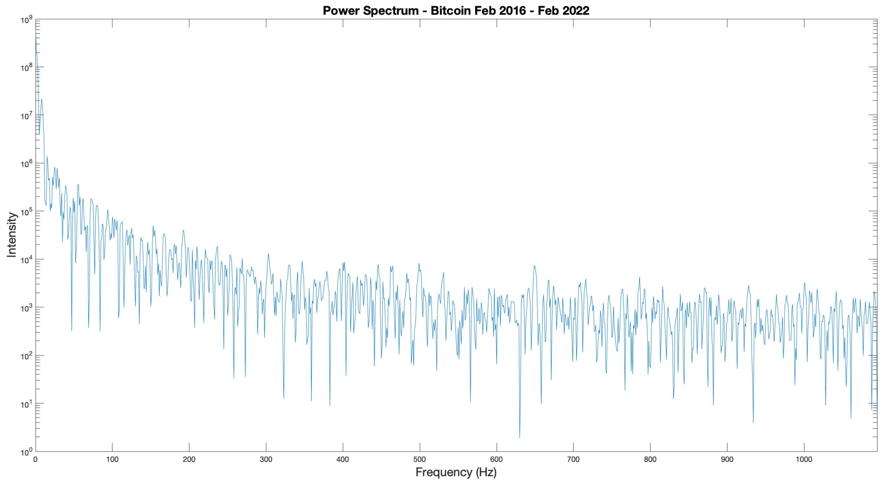
Figure 7.
Auto-correlation function output for absolute log price changes of the BTC-USD (2016-2022).
Figure 7.
Auto-correlation function output for absolute log price changes of the BTC-USD (2016-2022).
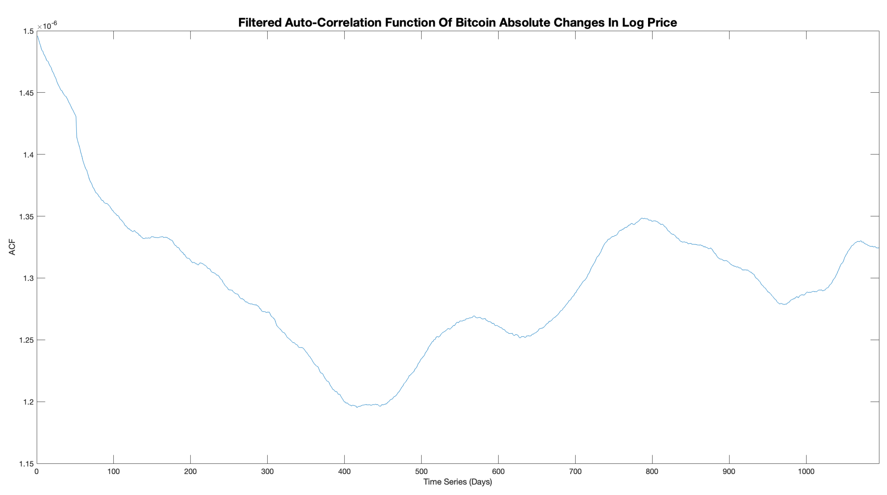
Figure 8.
Example graphical output of the backtesting function displaying - in green, in blue, filtered price data in red and the unfiltered price data in black. The right hand plot shows the unfiltered data on its original scale for comparison.
Figure 8.
Example graphical output of the backtesting function displaying - in green, in blue, filtered price data in red and the unfiltered price data in black. The right hand plot shows the unfiltered data on its original scale for comparison.
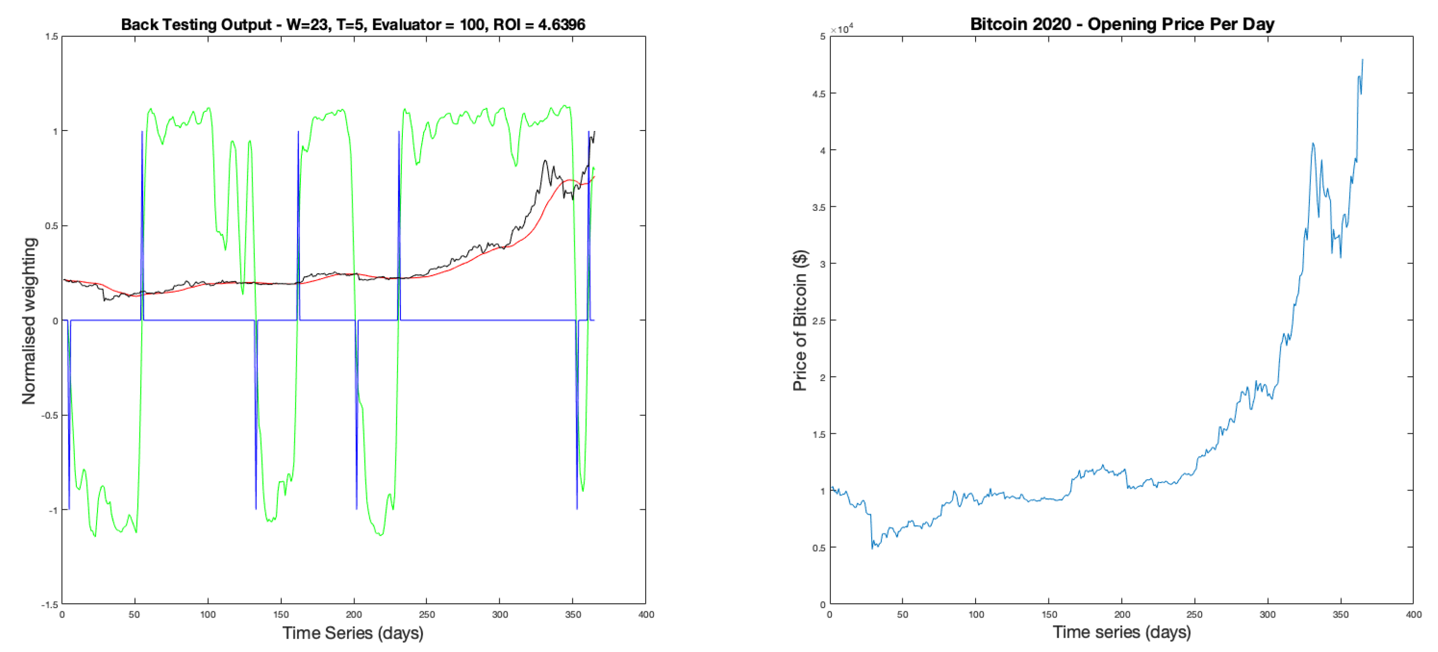
Figure 9.
Parameter optimisation for BTC-USD 2020-21 where x, z axis are W, T parameter combinations and the y axis is the evaluator output accuracy.
Figure 9.
Parameter optimisation for BTC-USD 2020-21 where x, z axis are W, T parameter combinations and the y axis is the evaluator output accuracy.
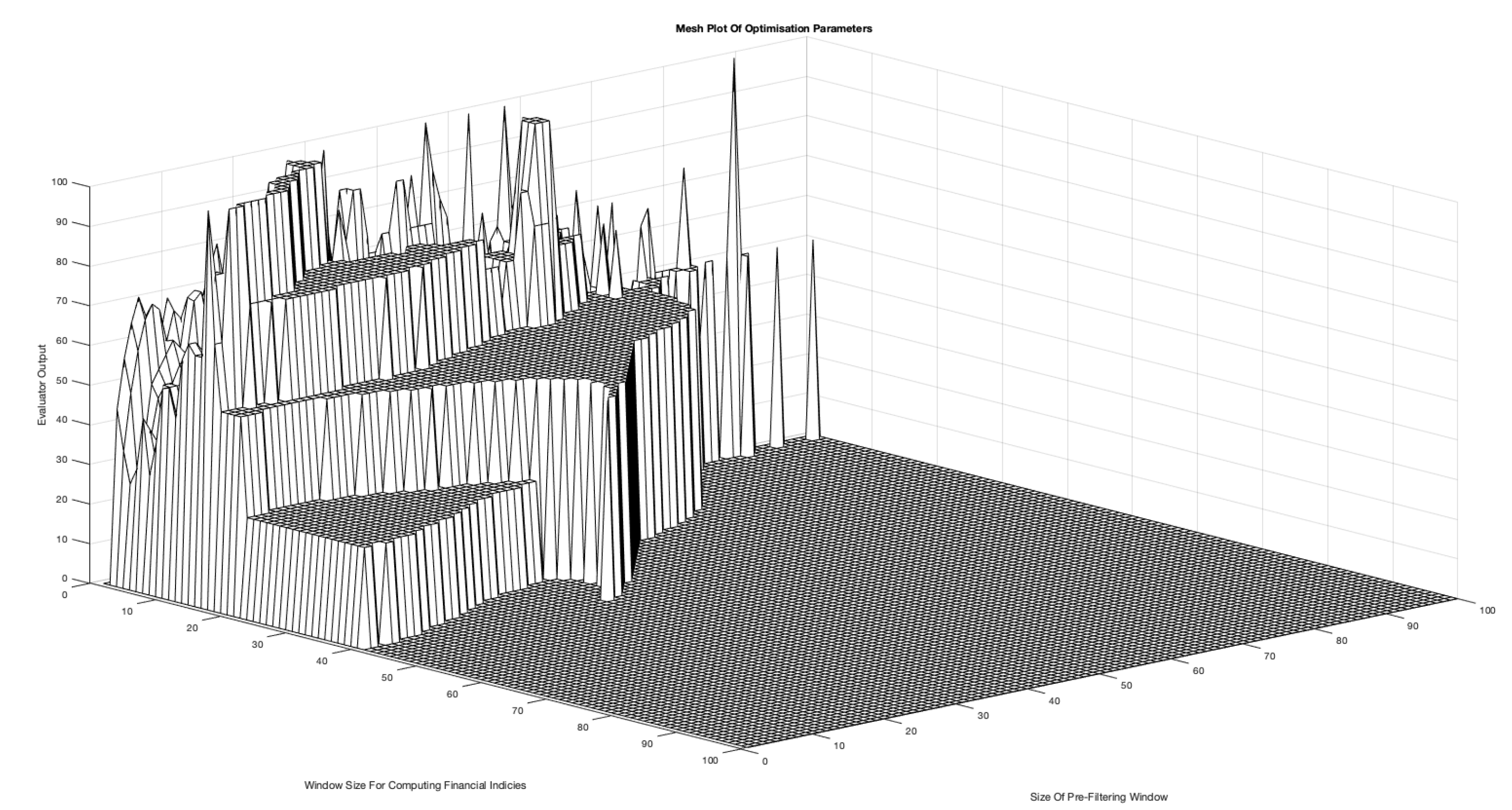
Figure 10.
Real BTC-USD prices compared to TuringBot trend fit equation for August 5th 2021 to September 10th 2021.
Figure 10.
Real BTC-USD prices compared to TuringBot trend fit equation for August 5th 2021 to September 10th 2021.
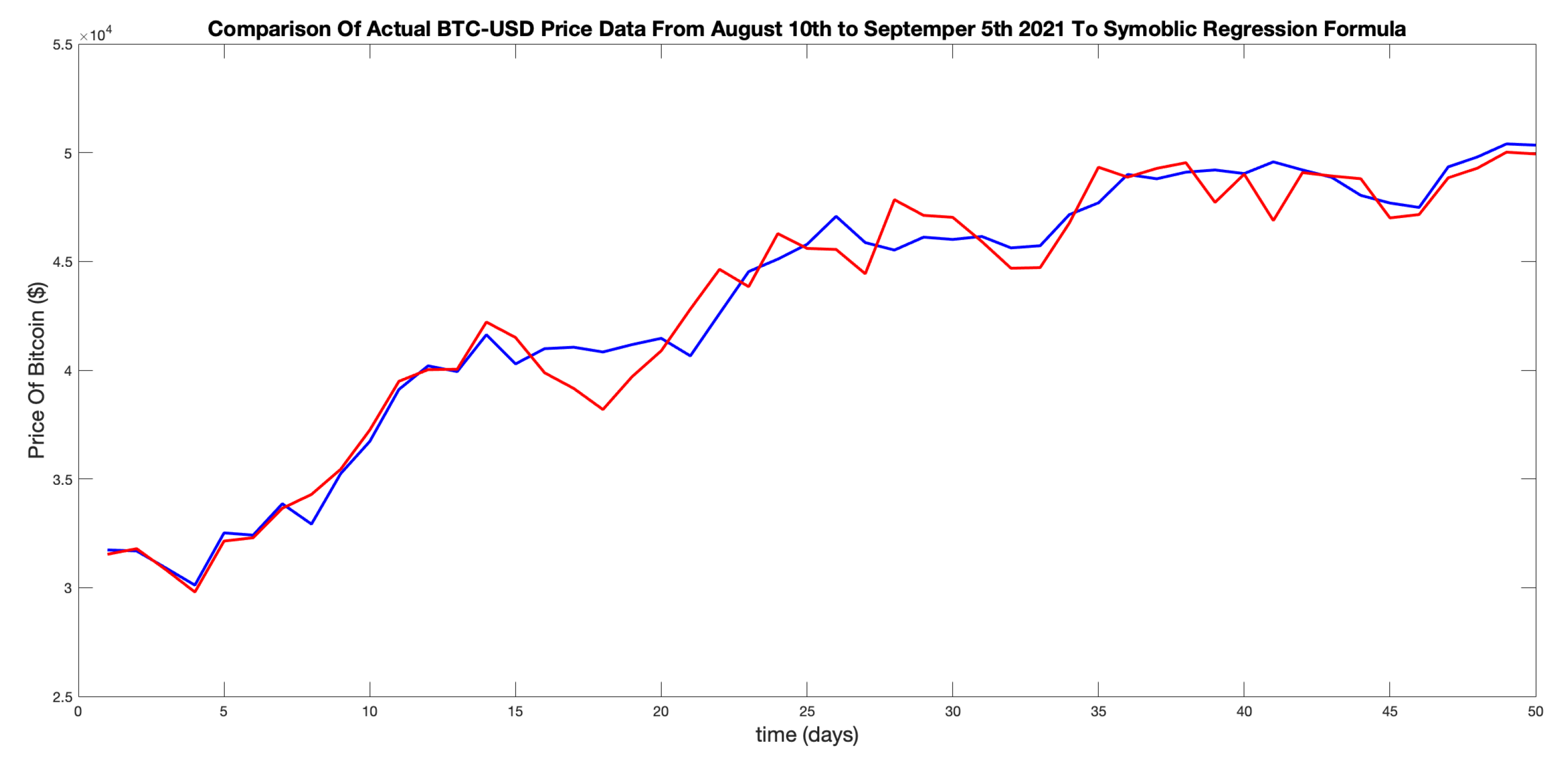
Figure 11.
Mesh plot for parameter optimisation of BTCUSD 2021-22.
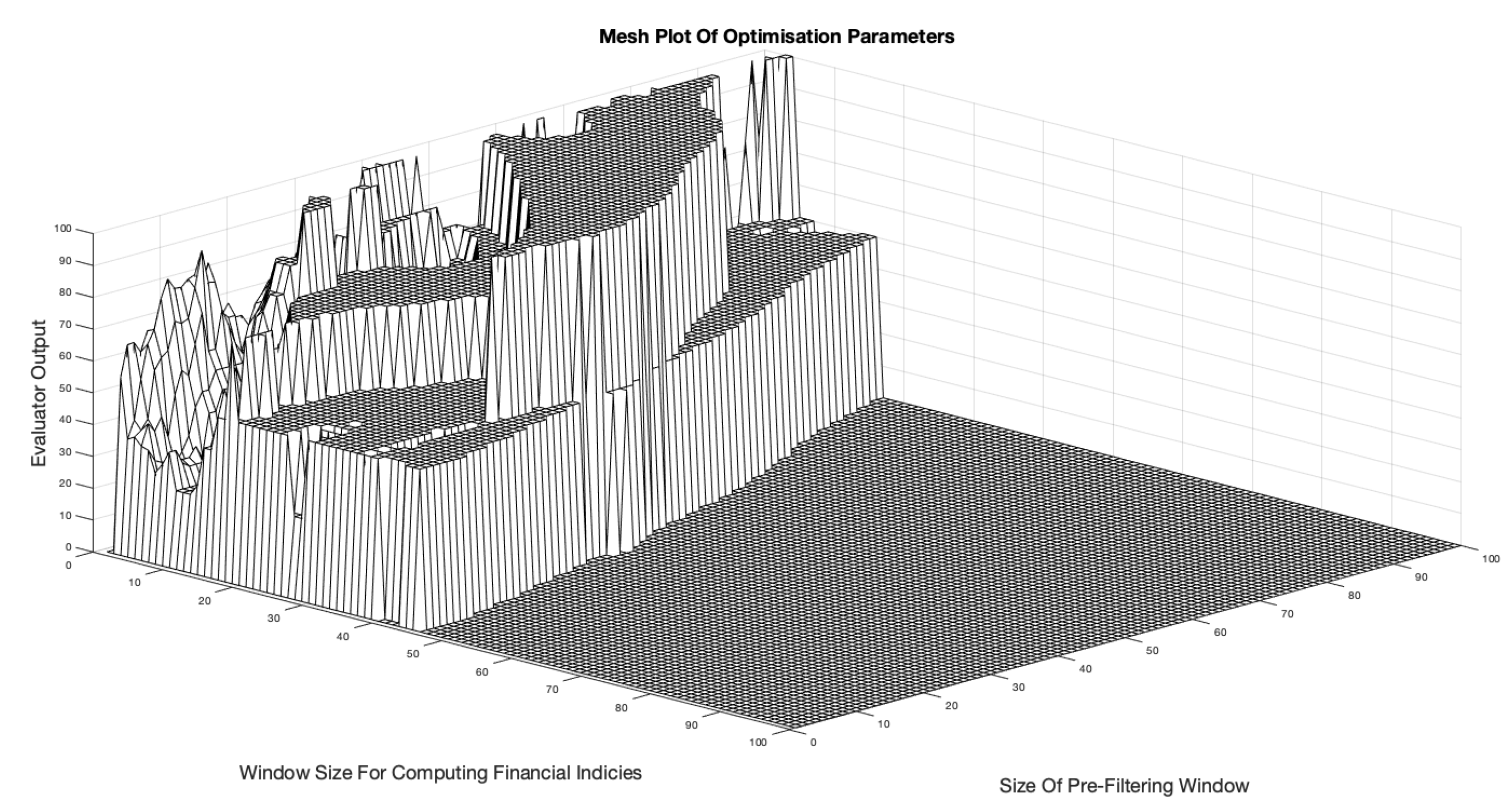
Figure 12.
Comparison Of backtesting metric signals for financial calculation windows, (red) (blue) with normalised price signal (black).
Figure 12.
Comparison Of backtesting metric signals for financial calculation windows, (red) (blue) with normalised price signal (black).
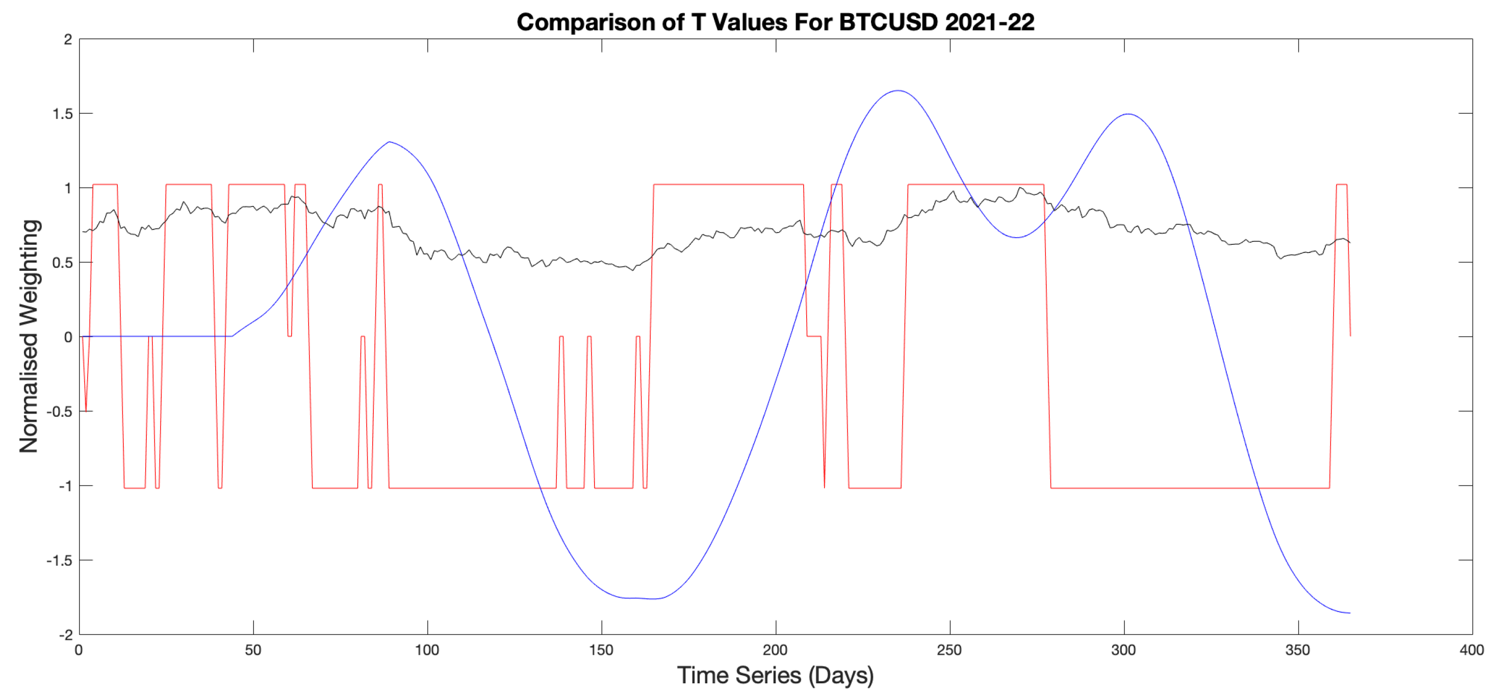
Figure 13.
Mesh plot of Return On Investment (ROIs) For BTC-USD 2021-22 optimum parameter positions where x, z axis represents W, T values respectively and y axis represents the % ROI.
Figure 13.
Mesh plot of Return On Investment (ROIs) For BTC-USD 2021-22 optimum parameter positions where x, z axis represents W, T values respectively and y axis represents the % ROI.
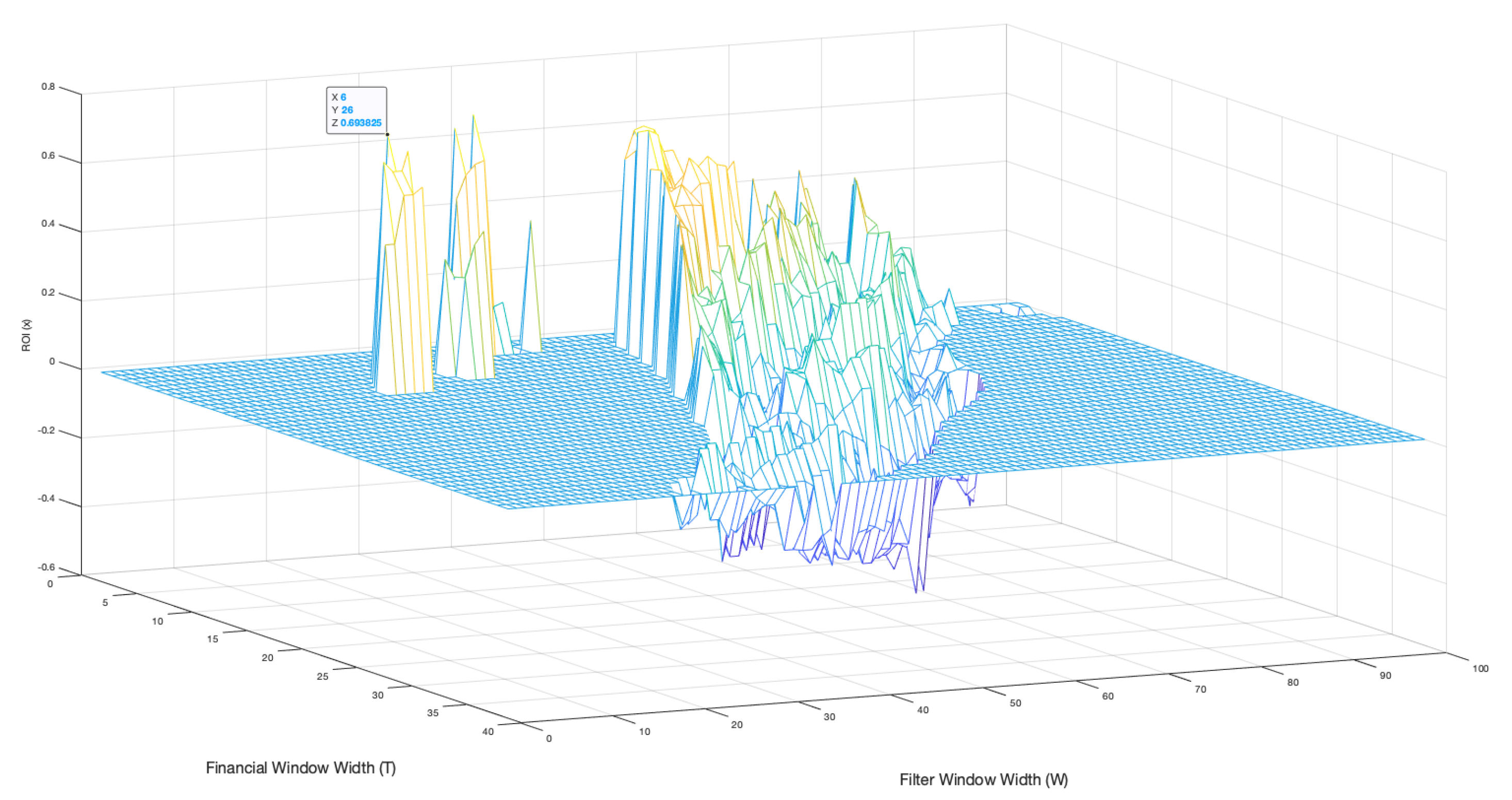
Figure 14.
Mesh plot of percentage Return On Investment (ROIs) for BTCUSD 2021-22 including all W, T parameter combinations.
Figure 14.
Mesh plot of percentage Return On Investment (ROIs) for BTCUSD 2021-22 including all W, T parameter combinations.
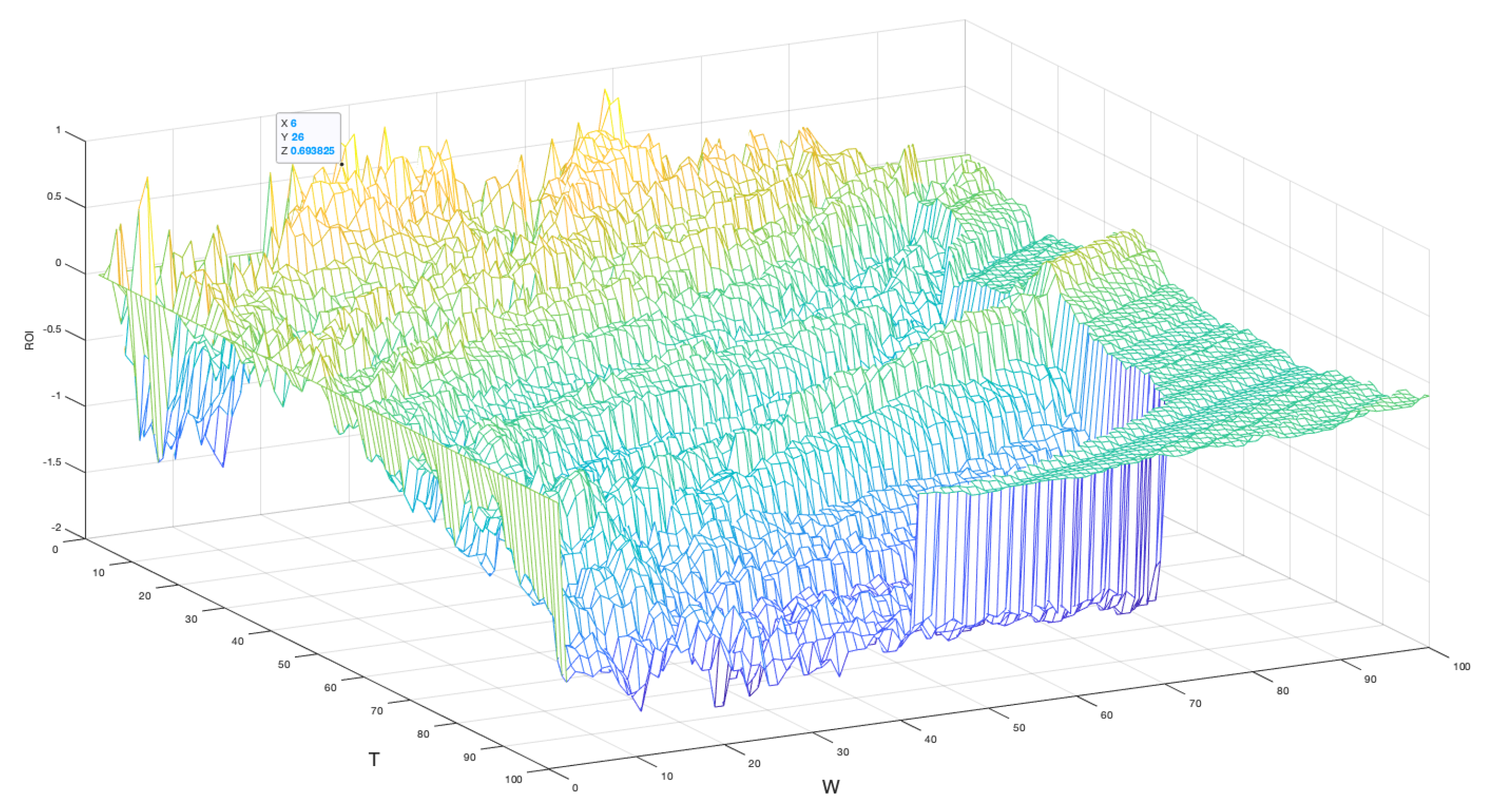
Figure 15.
`Top Down’ view of optimised parameter mesh plot showing only W, T combinations that achieve 100% accuracy for BTC-USD 2021-22.
Figure 15.
`Top Down’ view of optimised parameter mesh plot showing only W, T combinations that achieve 100% accuracy for BTC-USD 2021-22.
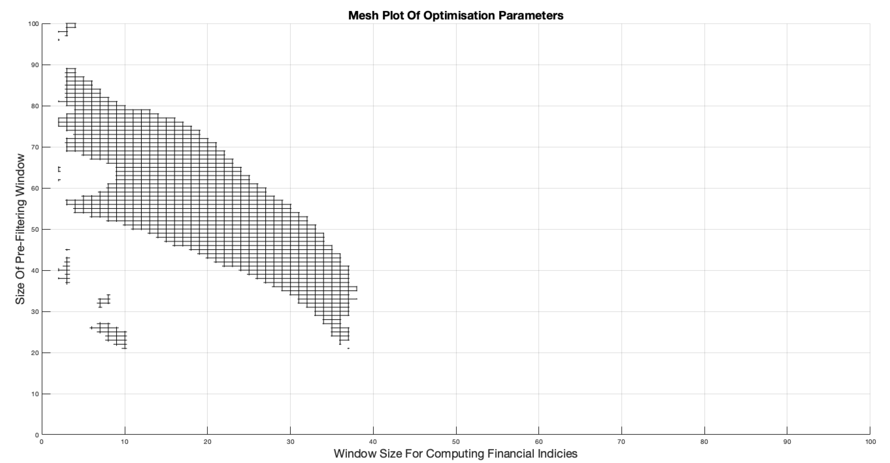
Figure 16.
Optimisation graphical output depicting `Top Down’ view of optimum parameter combinations (left) and Return On Investment (ROIs) for BTS-USD 2020-21.
Figure 16.
Optimisation graphical output depicting `Top Down’ view of optimum parameter combinations (left) and Return On Investment (ROIs) for BTS-USD 2020-21.
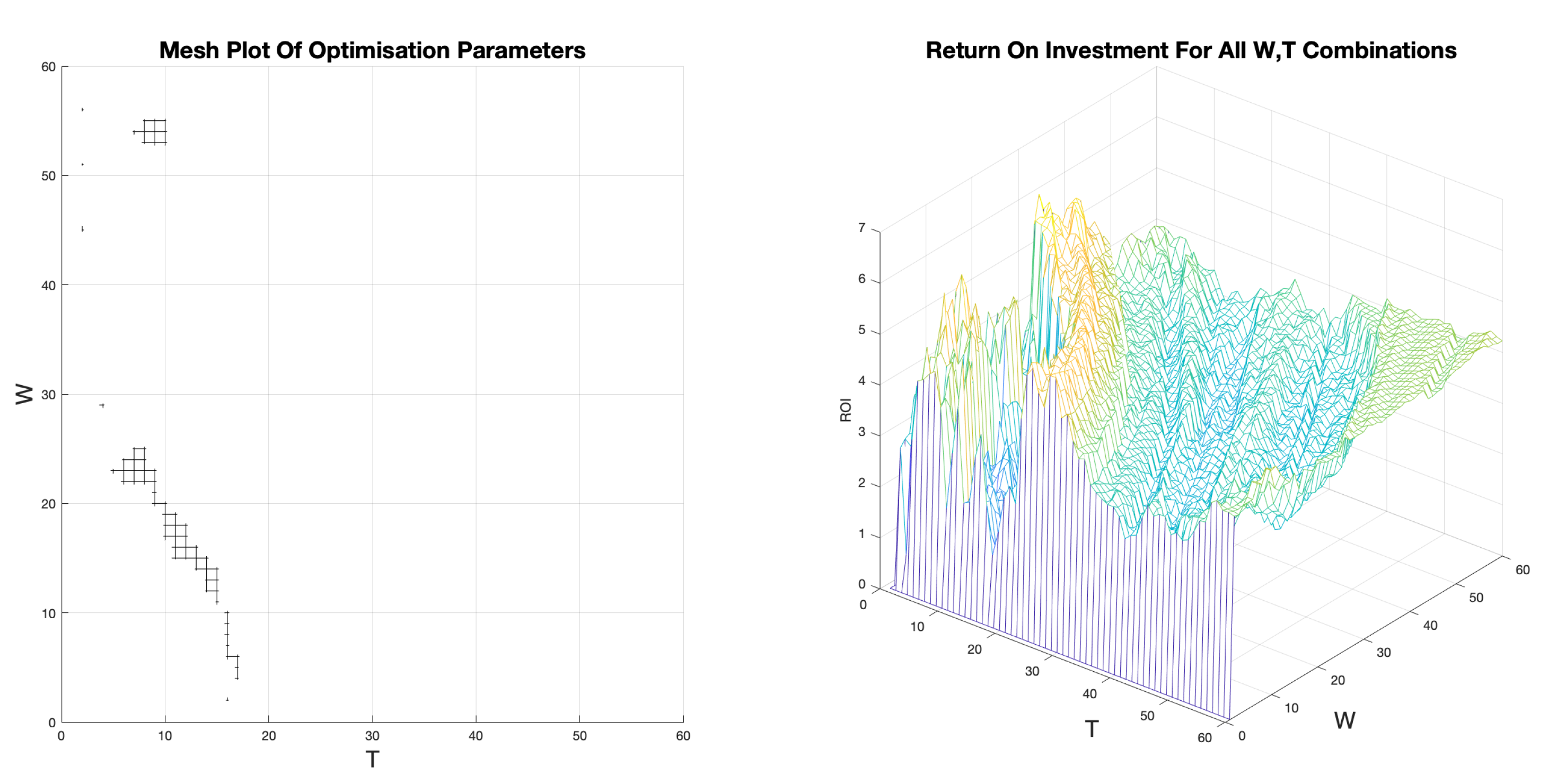
Figure 17.
Backtesting for BTCUSD 2021-22 with parameters , .
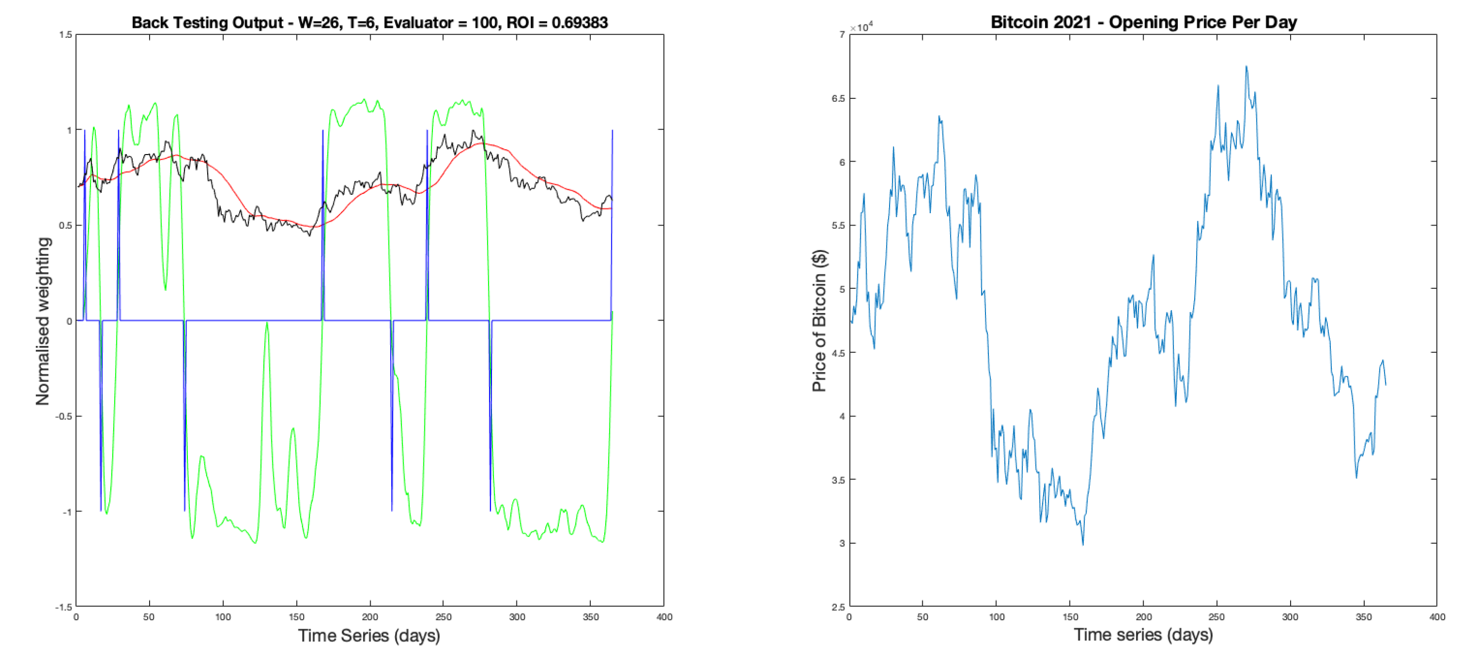
Figure 18.
20 days of hourly opening price data For BTC-USD.
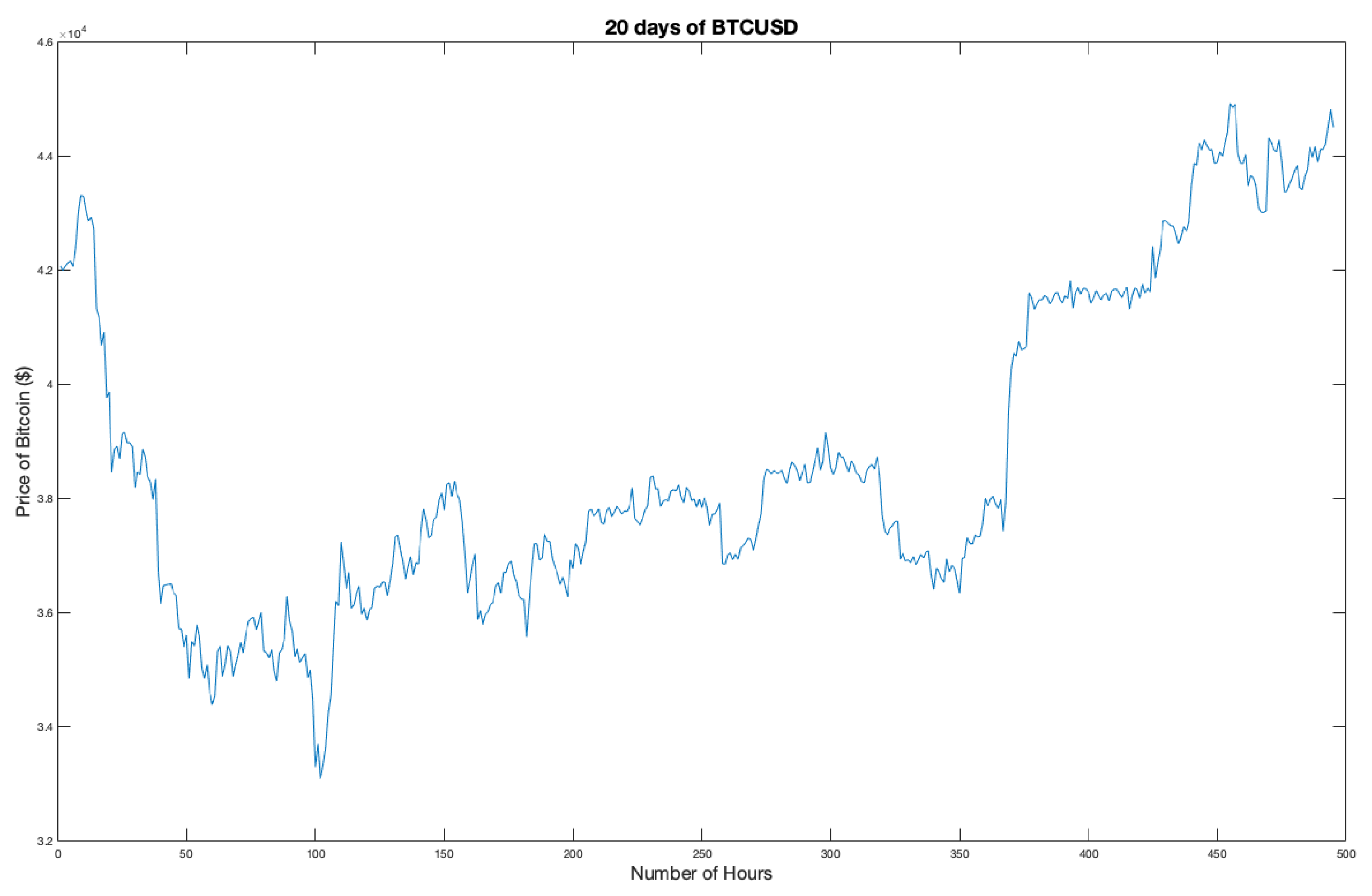
Figure 19.
Parameter optimisation mesh for BTC-USD Jan-Feb 2022.
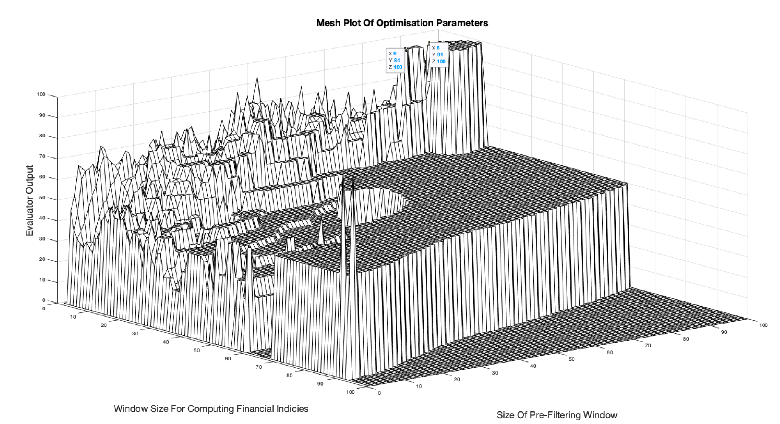
Figure 20.
`Top Down’ view of optimised parameter mesh plot showing only W, T combinations that achieve 100% accuracy for BTC-USD Jan-Feb 2022.
Figure 20.
`Top Down’ view of optimised parameter mesh plot showing only W, T combinations that achieve 100% accuracy for BTC-USD Jan-Feb 2022.
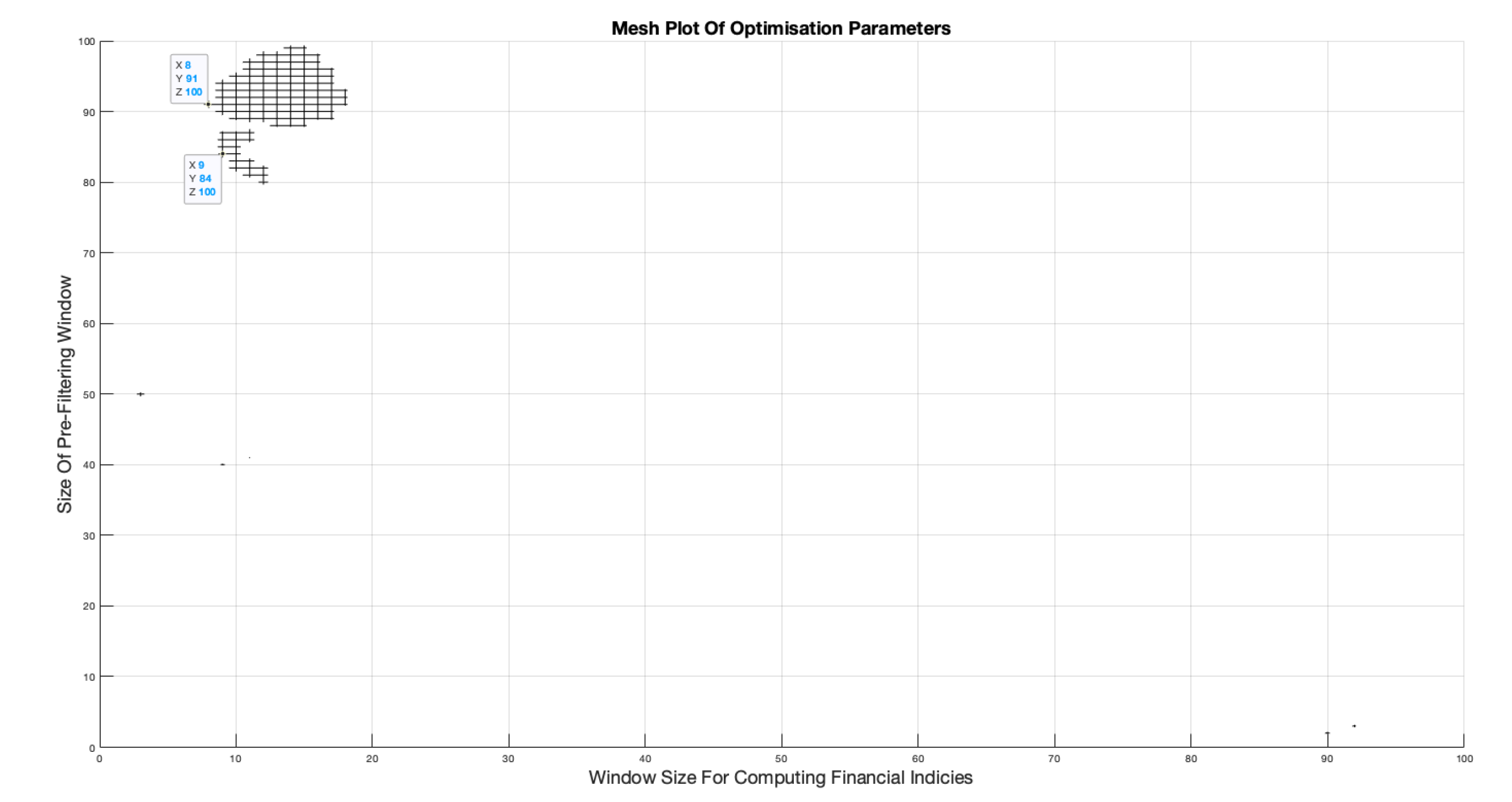
Figure 21.
Mesh plot of percentage Return On Investment (ROIs) for BTC-USD Jan-Feb 2022.
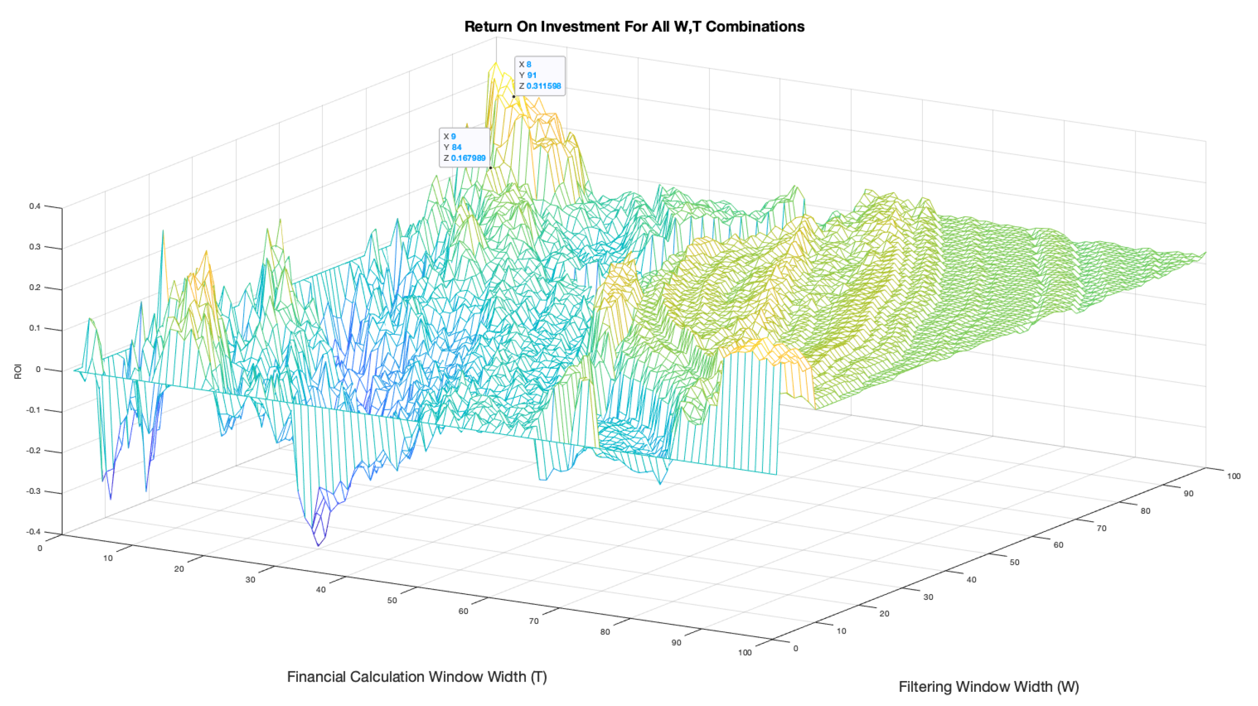
Figure 22.
Backtesting output comparison of two invalid combinations - (left) and (right).
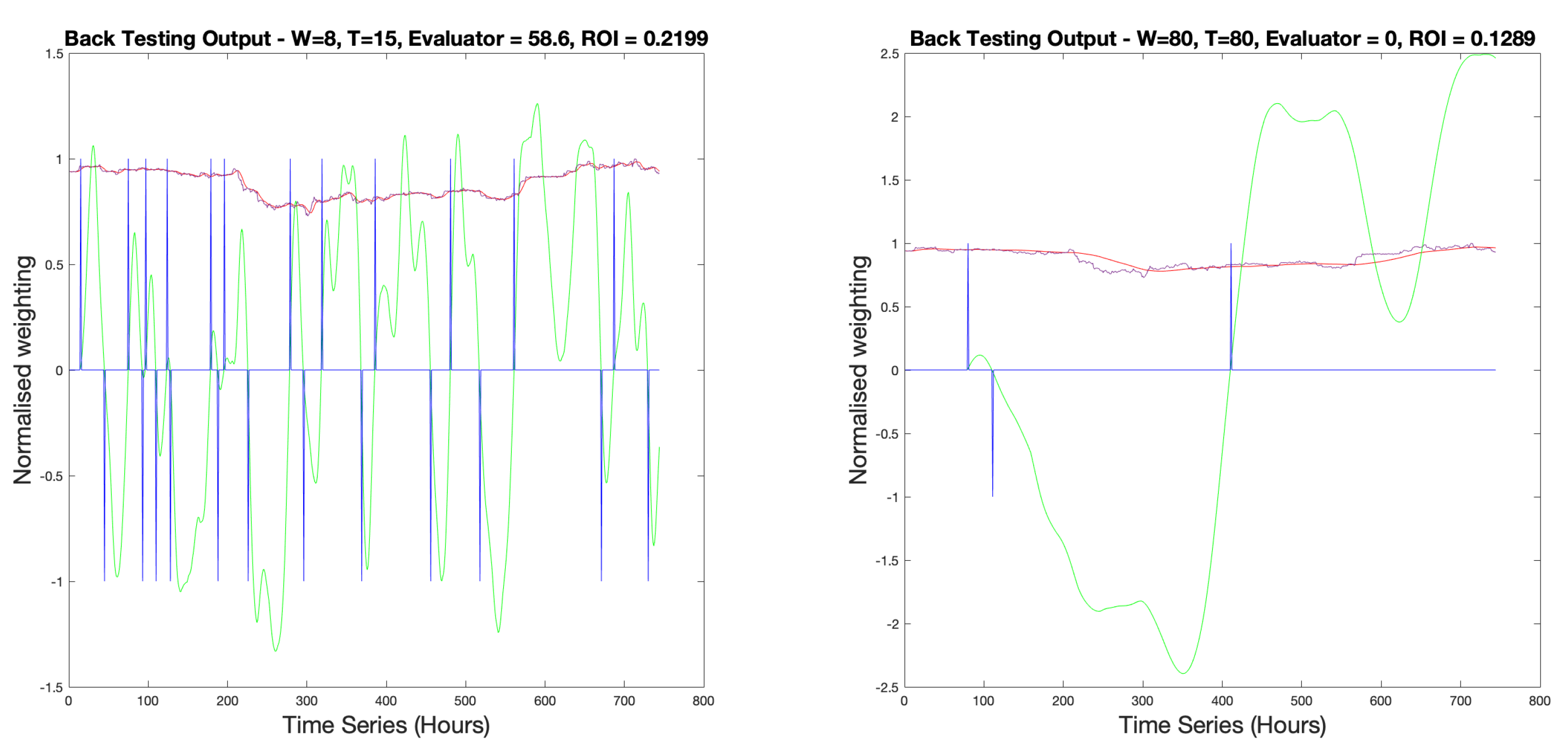
Figure 23.
Backtesting for BTCUSD Jan-Feb 2022 with parameters .
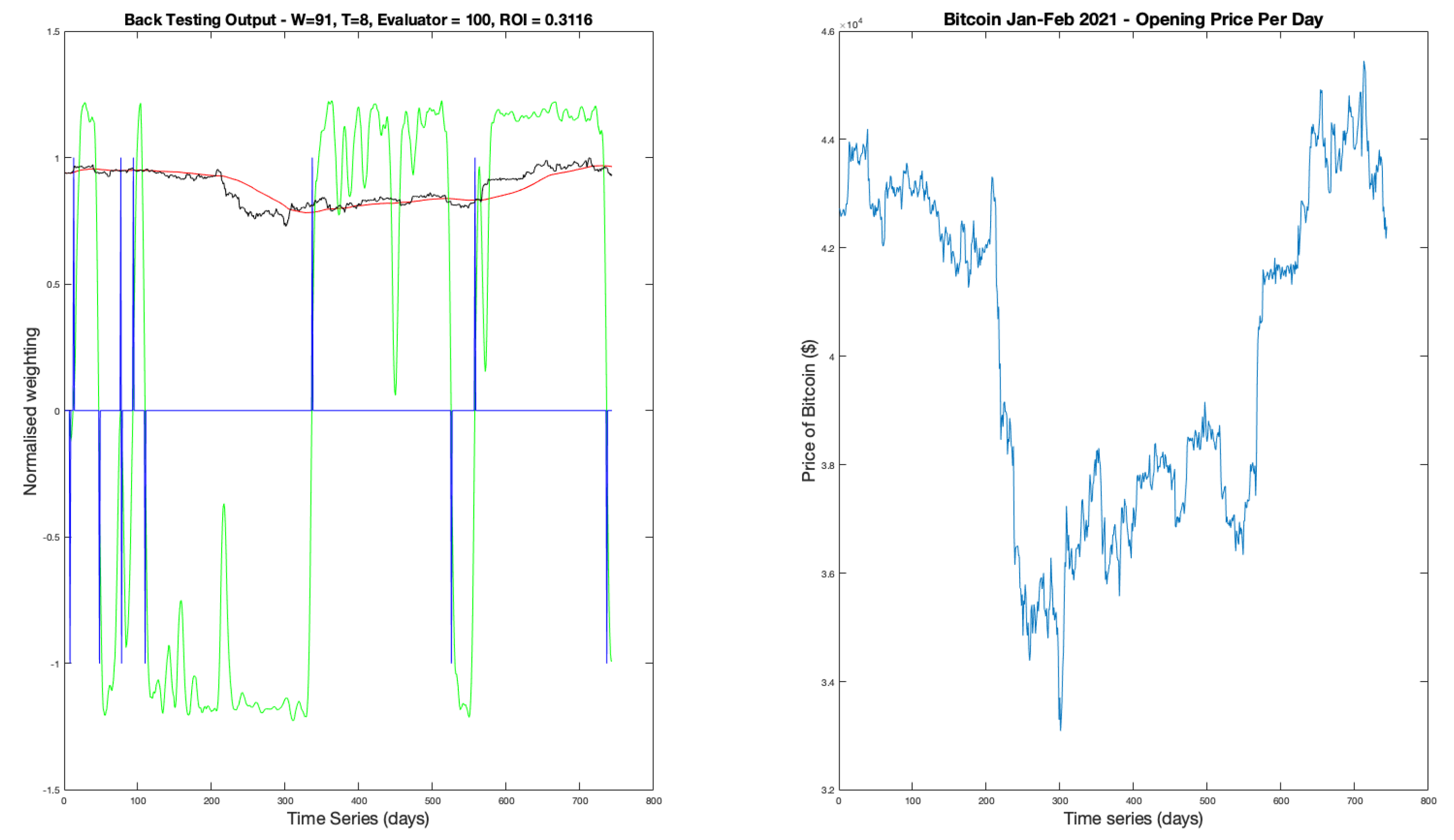
Figure 24.
Backtesting for BTCUSD 2021-22 using LVR with parameters .
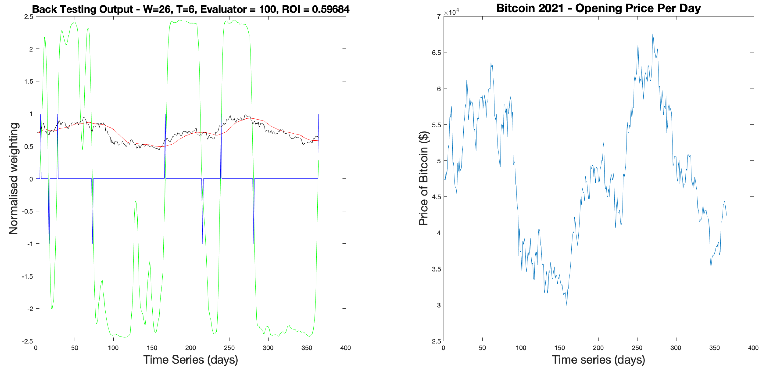
Figure 25.
Price prediction using symbolic regression for BTC-USD Aug 21st to Sep 10th with price estimation from Sep 11th to Sep 20th (+10 days).
Figure 25.
Price prediction using symbolic regression for BTC-USD Aug 21st to Sep 10th with price estimation from Sep 11th to Sep 20th (+10 days).
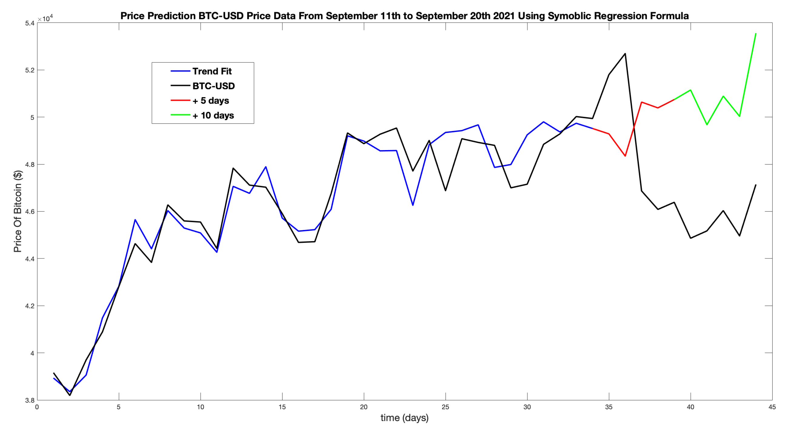
Figure 26.
Price prediction using symbolic regression for BTC-USD for look-back window lengths of (top) and (bottom).
Figure 26.
Price prediction using symbolic regression for BTC-USD for look-back window lengths of (top) and (bottom).
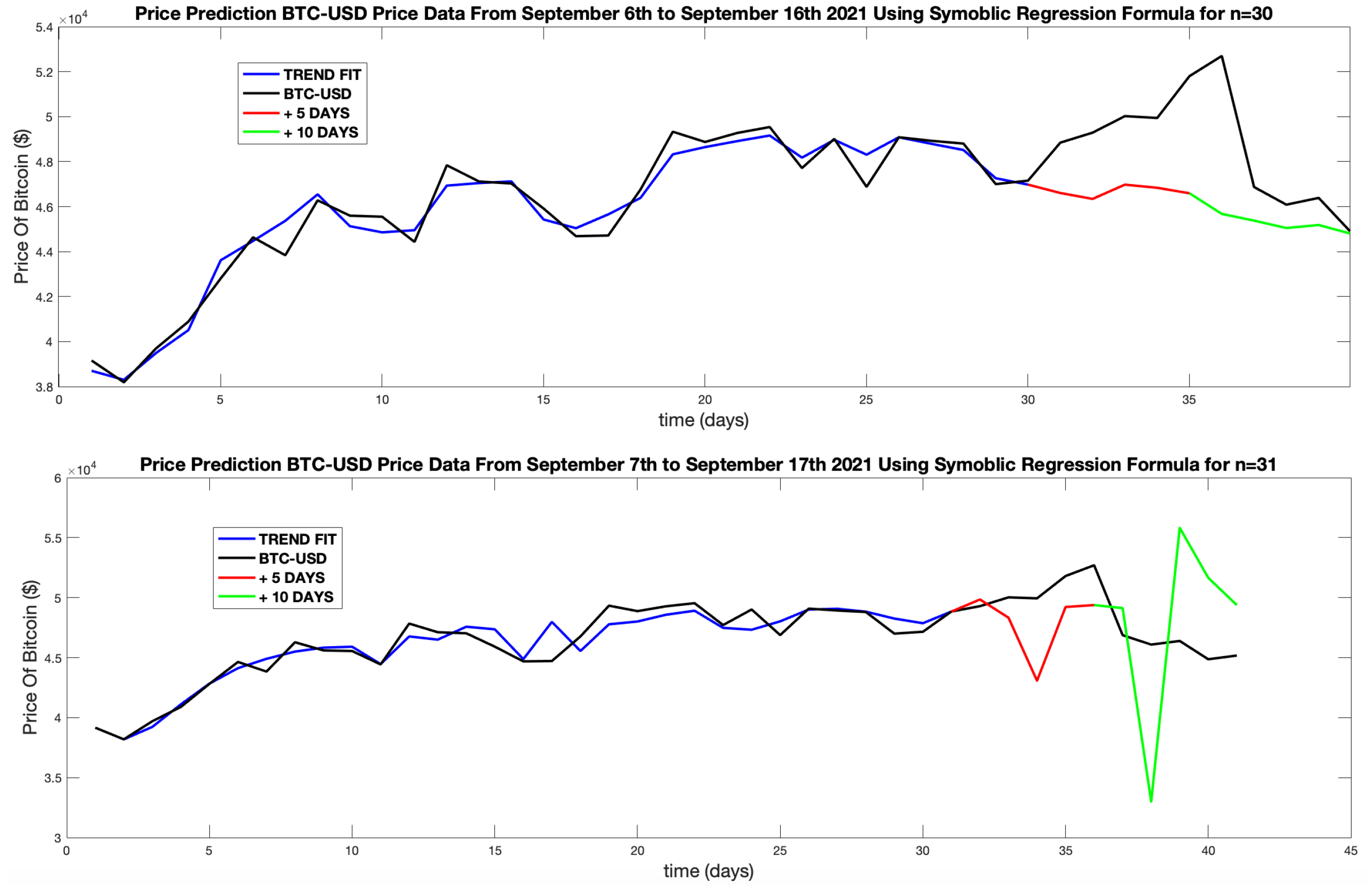
Figure 27.
Price prediction using symbolic regression for BTC-USD Aug 18th to Sep 7th with price estimation from Sep 7th to Sep 17th (+10 days).
Figure 27.
Price prediction using symbolic regression for BTC-USD Aug 18th to Sep 7th with price estimation from Sep 7th to Sep 17th (+10 days).
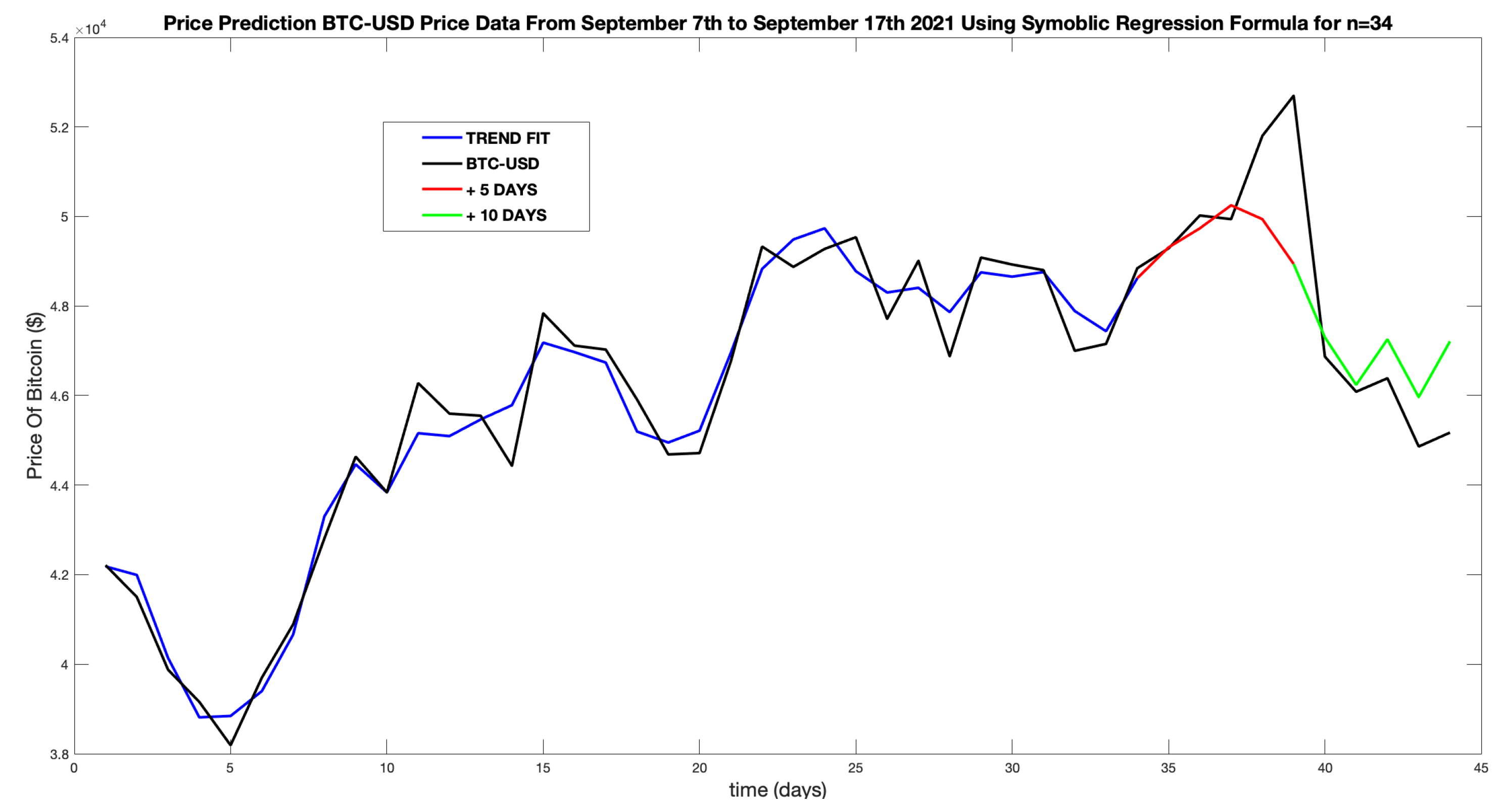
Figure 28.
Price prediction using symbolic regression for BTC-USD Aug 2nd to Sep 7th with price estimation from Sep 7th to Sep 15th (+8 days).
Figure 28.
Price prediction using symbolic regression for BTC-USD Aug 2nd to Sep 7th with price estimation from Sep 7th to Sep 15th (+8 days).
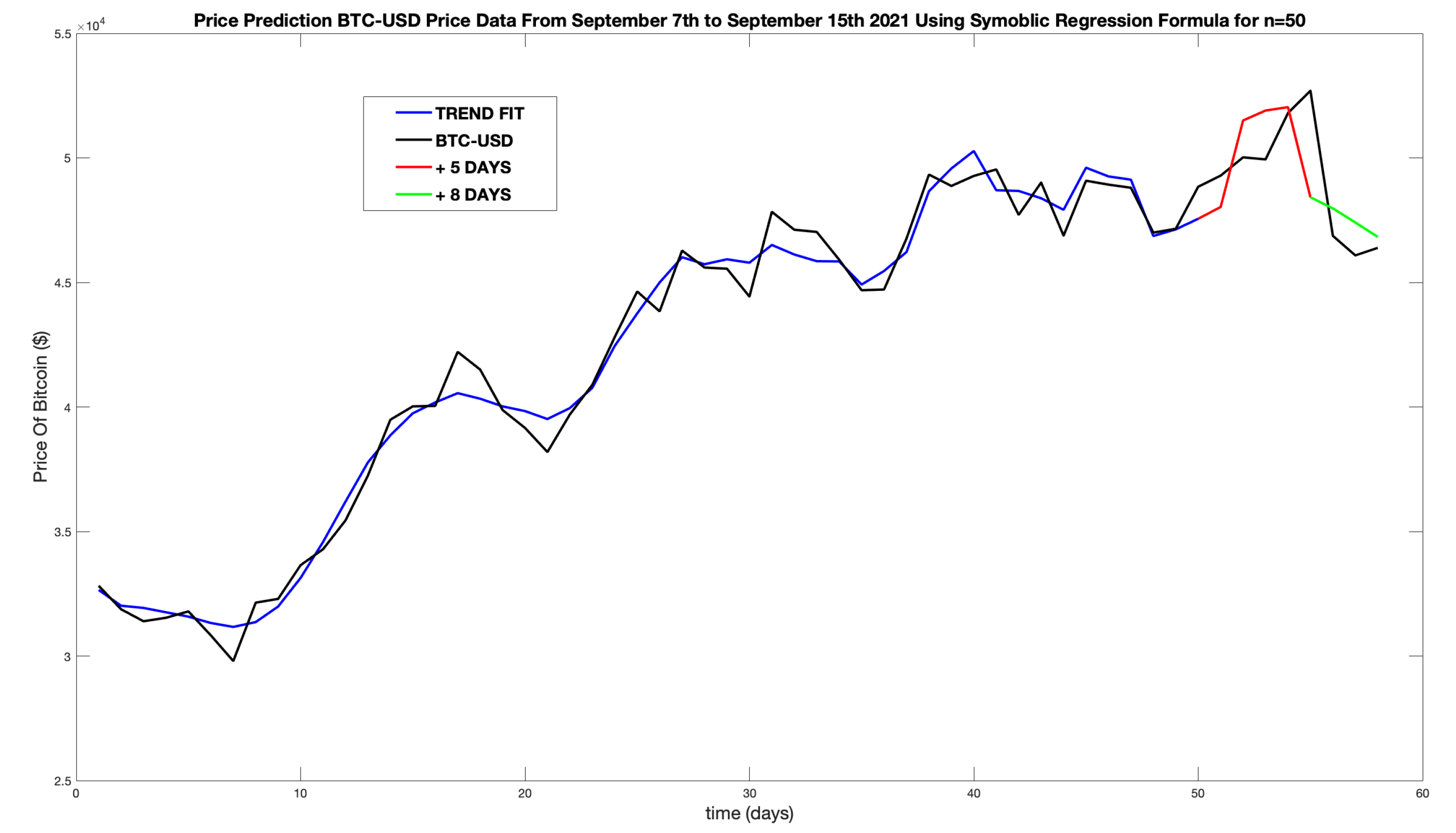
Figure 29.
Log-Log power spectrum for BTC-USD Feb 2016-2022.
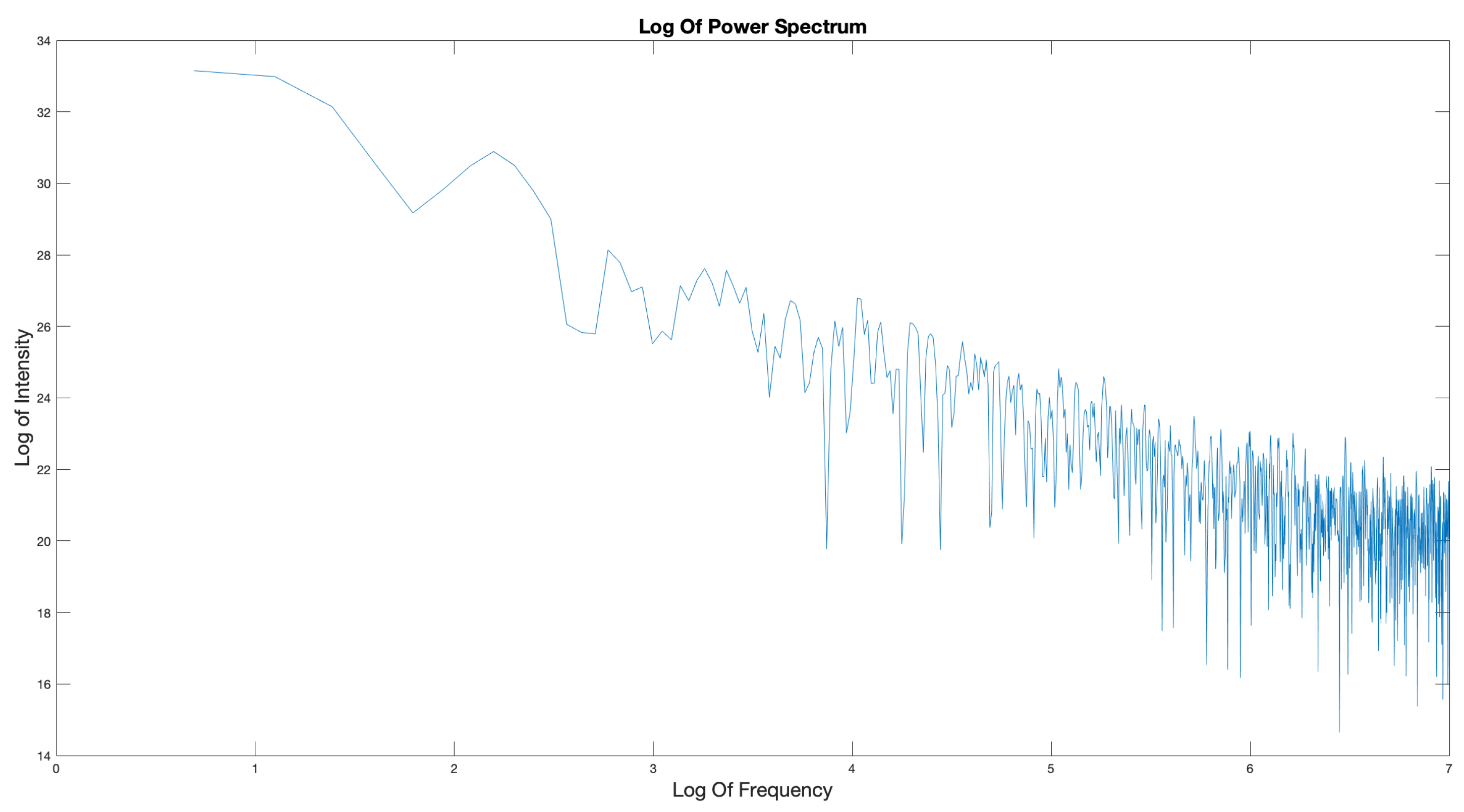
Figure 30.
Comparison between daily and hourly system outputs for BTC-USD Jan-Feb 2022.
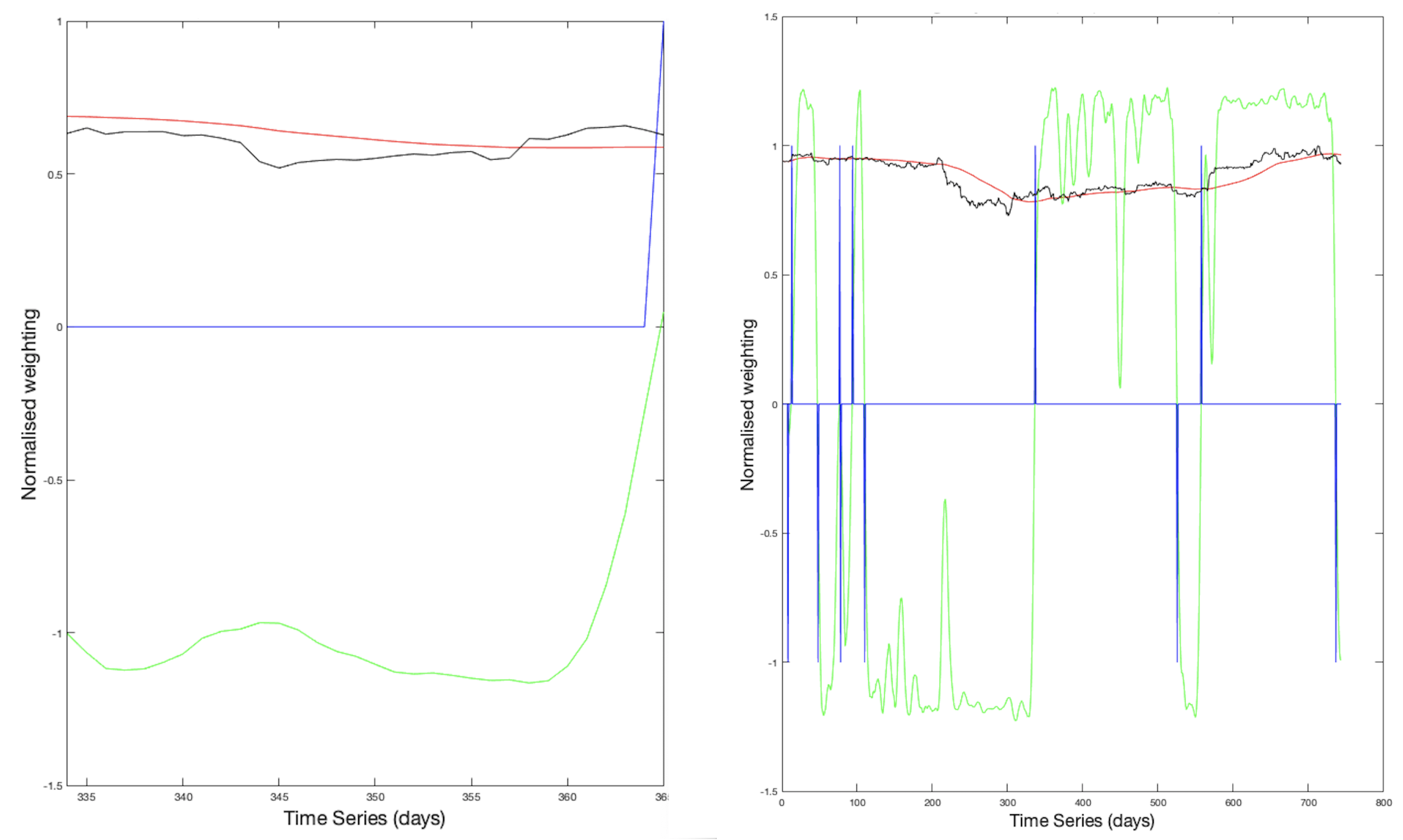
Table 1.
Comparison of BTC-USD and ETH-USD fractal indexes for both daily and hourly time series (2016-2022).
Table 1.
Comparison of BTC-USD and ETH-USD fractal indexes for both daily and hourly time series (2016-2022).
| Index | BTC-USD | ETH-USD | BTC-USD | ETH-USD |
|---|---|---|---|---|
| Daily | Daily | Hourly | Hourly | |
| Spectral Decay () | 0.8185 | 0.8232 | 0.8714 | 0.8895 |
| Hurst Exponent (H) | 0.3185 | 0.3232 | 0.3732 | 0.3895 |
| Fractal Dimension () | 1.6815 | 1.6768 | 1.6286 | 1.6105 |
| Levy Index () | 1.2218 | 1.2142 | 1.1452 | 1.1242 |
Table 2.
List of financial time series.
| Name | Start | End | Time Step | Data Points |
|---|---|---|---|---|
| BTCUSD2021 | 12-02-2021 | 12-02-2022 | 24 | 365 |
| BTCUSD2020 | 12-02-2020 | 12-02-2021 | 24 | 365 |
| BTCUSD2019 | 12-02-2019 | 12-02-2020 | 24 | 365 |
| BTCUSD2018 | 12-02-2018 | 12-02-2019 | 24 | 365 |
| BTCUSD2017 | 12-02-2017 | 12-02-2018 | 24 | 365 |
| BTCUSD2016 | 12-02-2016 | 12-02-2017 | 24 | 365 |
| BTCUSD_janfeb | 12-02-2016 | 12-02-2017 | 1 | 744 |
| BTCUSD_decjan | 12-02-2016 | 12-02-2017 | 1 | 744 |
| BTCUSD_novdec | 12-02-2016 | 12-02-2017 | 1 | 720 |
Table 3.
Percentage return on investment of BTC-USD and ETH-USD for daily financial time series using Beta-to-Volatility ratio.
Table 3.
Percentage return on investment of BTC-USD and ETH-USD for daily financial time series using Beta-to-Volatility ratio.
| Year | BTC-USD | ETH-USD | ||||||
|---|---|---|---|---|---|---|---|---|
| W | T | Evaluator (%) | ROI (%) | W | T | Evaluator (%) | ROI (%) | |
| 2016-17 | 33 | 8 | 100 | 194 | NA | NA | NA | NA |
| 2017-18 | 23 | 8 | 100 | 2,487 | 17 | 3 | 100 | 11,093 |
| 2018-19 | 20 | 3 | 87.5 | 38.5 | 21 | 3 | 100 | 76 |
| 2019-20 | 43 | 4 | 100 | 267 | 17 | 3 | 94.4 | 108 |
| 2020-21 | 23 | 5 | 100 | 464 | 15 | 5 | 100 | 1,207 |
| 2021-22 | 26 | 6 | 100 | 69 | 27 | 6 | 100 | 264 |
Table 4.
Percentage return on investment of BTC-USD and ETH-USD for hourly financial time series using Beta-to-Volatility ratio.
Table 4.
Percentage return on investment of BTC-USD and ETH-USD for hourly financial time series using Beta-to-Volatility ratio.
| Year | BTC-USD | ETH-USD | ||||||
|---|---|---|---|---|---|---|---|---|
| W | T | Evaluator (%) | ROI (%) | W | T | Evaluator (%) | ROI (%) | |
| Nov-Dec | 44 | 10 | 100 | 11.8 | 50 | 7 | 100 | 27.2 |
| Dec-Jan | 90 | 7 | 83.3 | 20 | 73 | 9 | 100 | 15.5 |
| Jan-Feb | 91 | 8 | 100 | 31.1 | 85 | 10 | 100 | 51.1 |
Table 5.
Percentage return on investment of BTC-USD and ETH-USD for daily financial time series using the Lyapunov-to-Volatility (LVR) ratio.
Table 5.
Percentage return on investment of BTC-USD and ETH-USD for daily financial time series using the Lyapunov-to-Volatility (LVR) ratio.
| Year | BTC-USD (%) | ETH-USD (%) |
|---|---|---|
| 2016-17 | 137 | NA |
| 2017-18 | 2,248 | 10,425 |
| 2018-19 | 40.6 | 62.7 |
| 2019-20 | 248 | 119.9 |
| 2020-21 | 456 | 1,158 |
| 2021-22 | 59.7 | 248 |
Table 6.
Percentage return on investment of BTC-USD and ETH-USD for daily financial time series using both LVR and BVR indicators compared to Buy & Hold strategy (B&H).
Table 6.
Percentage return on investment of BTC-USD and ETH-USD for daily financial time series using both LVR and BVR indicators compared to Buy & Hold strategy (B&H).
| Year | BTC-USD | ETH-USD | ||||
|---|---|---|---|---|---|---|
| ROI - | ROI - | B&H (%) | ROI - | ROI - | B&H (%) | |
| 2016-17 | 137 | 194 | 162 | NA | NA | NA |
| 2017-18 | 2,248 | 2,487 | 700 | 10,425 | 11,093 | 7,021 |
| 2018-19 | 40.6 | 38.5 | -60 | 62.7 | 76 | -86.2 |
| 2019-20 | 248 | 267 | 185 | 119.9 | 108 | 95.1 |
| 2020-21 | 456 | 465 | 369 | 1,158 | 1,207 | 565 |
| 2021-22 | 59.7 | 69 | -10.7 | 248 | 264 | 58.7 |
Disclaimer/Publisher’s Note: The statements, opinions and data contained in all publications are solely those of the individual author(s) and contributor(s) and not of MDPI and/or the editor(s). MDPI and/or the editor(s) disclaim responsibility for any injury to people or property resulting from any ideas, methods, instructions or products referred to in the content. |
© 2025 by the authors. Licensee MDPI, Basel, Switzerland. This article is an open access article distributed under the terms and conditions of the Creative Commons Attribution (CC BY) license (http://creativecommons.org/licenses/by/4.0/).
Copyright: This open access article is published under a Creative Commons CC BY 4.0 license, which permit the free download, distribution, and reuse, provided that the author and preprint are cited in any reuse.


