
Submitted:
14 July 2024
Posted:
15 July 2024
You are already at the latest version
Abstract
This article comprehensively explores multiple aspects of cryptocurrencies and their price forecasting. Firstly, the article introduces the definition of cryptocurrency and its development process on a global scale, especially focusing on the launch of Facebook Libra and China's central bank digital currency, highlighting the importance and influence of digital currency in the global financial market. Subsequently, the article analyzes the advantages of digital currencies over traditional currencies, including improving economic transaction efficiency, reducing transaction costs and enhancing transaction transparency. Meanwhile, the article also explores the challenges and risks potentially brought by the development of digital currencies, such as regulatory uncertainty and market volatility. In this context, the article raises the importance of cryptocurrency price forecasting and introduces the forecasting models and techniques commonly used today. Finally, through specific experimental analysis, the effectiveness of using the deep learning model CNN-LSTM to predict the price of Bitcoin is demonstrated, and the directions of future research and optimization strategy are proposed. In summary, this paper comprehensively presents the research status and prospects of cryptocurrency and its price prediction field through systematic introduction and analysis.
Keywords:
Cryptocurrencies
; price forecasting
; artificial intelligence
; deep learning
; financial technology
1. Introduction
Cryptocurrency is a kind of virtual currency based on cryptography algorithm and generated by computer operations. Since 2009, thousands of cryptocurrencies have come out around the world, which have aroused the general concern of investors and central banks. On June 18, 2019, the social media company Facebook (now Meta) released a white paper on the cryptocurrency Libra (now renamed to Diem) based on blockchain technology. Through technological innovation, Libra has the characteristics of stability, low inflation and so on, and can be used for payment of daily transactions [1]. The People’s Bank of China began pilot activities for the implementation of the central bank’s fiat digital currency in October 2020.
The price of cryptocurrency can be affected by various economic, political and other factors. The price fluctuation is huge and difficult to predict. Therefore, the research on its price forecast in this paper can provide some valuable suggestions for investors to avoid risks and increase investment returns.
Blockchain technology, pioneered by Bitcoin, has captured widespread attention and ignited discussions on its potential applications. This breakthrough innovation holds promise for revolutionizing various aspects of the digital economy and expediting the development of central bank digital currencies (CBDCs) [2]. As blockchain continues to evolve rapidly, the proliferation of cryptocurrencies is anticipated globally. To safeguard China’s financial security and advance the internationalization of the RMB, it is imperative to conduct thorough research on cryptocurrencies.
Cryptocurrencies have the potential to play significant roles in cross-border payments, foreign trade, and combating financial crimes. However, the empirical research on cryptocurrencies in China is still in its nascent stages. It is crucial to delve into the intrinsic value characteristics of cryptocurrencies and understand their price fluctuation patterns [3]. By doing so, valuable insights can be gleaned to inform policy decisions and provide recommendations to relevant government agencies.
In exploring the potential applications of cryptocurrencies, particular attention should be given to their impact on cross-border transactions. The decentralized nature of cryptocurrencies presents opportunities to streamline international payments, reduce transaction costs, and enhance efficiency. Additionally, cryptocurrencies can facilitate foreign trade by providing a secure, transparent, and efficient medium of exchange. By harnessing blockchain technology, China can optimize its trade processes and bolster its position in the global market.
2. Related Work
2.1. DIGICCY (Digital Currency)
A digital currency is an electronic currency, usually issued and managed by a developer, accepted and used by members of a particular virtual community. Unlike virtual currencies in virtual worlds, digital currencies can be used to buy real goods and services, not just online games. An early digital currency [4](digital gold currency) was a form of electronic money named after the weight of gold. Today’s digital currencies, such as Bitcoin, Litecoin, and PPCoin, rely on checksum and cryptography to create, issue, and circulate electronic money.
The emergence of digital currency is a product of the digital age, which breaks the physical form and geographical restrictions of traditional money, and provides convenience for transactions on a global scale. With the support of blockchain technology, the transaction records of digital currencies are securely stored and verified, making the transaction process more transparent and secure [5]. In addition, the decentralized nature of digital currencies makes them not controlled by any central authority, further enhancing the security and privacy of transactions.
As the digital currency market continues to grow, people’s understanding and application of it are also deepening [6]. More and more merchants are beginning to accept digital currency as a payment method, while investors are also starting to consider it as an investment objective. Risks and opportunities coexist in the digital currency market, so it is particularly important to study its related technology, market and regulation.
1. compared with paper money, digital currency has obvious advantages, not only can save the cost of issuance and circulation, but also improve the transaction speed and investment efficiency, and enhance the convenience and transparency of economic transaction activities.
2. Issuing digital currency can improve the convenience and transparency of economic transaction activities, and further reduce illegal and criminal acts such as money laundering and tax evasion. It enhances the central bank’s control over money supply and currency circulation, which better supports the economic and social development, and help the full realization of inclusive finance.
3. The issuance of digital currency by the central bank ensures the coherence of financial policy and the integrity of monetary policy, and also guarantees the safety of monetary transactions[7]. The central bank has also starting to consider the issues related to anti-counterfeiting and supervision of digital currencies. The central bank will cooperate with the financial and scientific and technological communities to further increase the research and rational use of various innovative technologies.
Therefore, the initial positioning of the digital RMB should be a digital legal currency that can supplement the existing electronic payment system and supplement the payment tools for people’s daily consumption. Since there are still large-scale paper forms of RMB circulating on the market, the central bank is not in a hurry to completely replace the digital RMB[8] paper currency, and it is clear that the two will coexist for a long time. Therefore, in terms of the daily use experience of the public, there is no difference between the two. For ordinary consumers at the C end, only the carrier form of the two is changed, while for commercial users at the B end, the transaction between them is still based on RMB. However, in the government affairs scenario at the G end, the transaction between them is still based on RMB. The transfer of relevant funds is conducted without any intermediaries, bypassing the local government’s oversight and effectively mitigating the corruption risks associated with middle-level bureaucracy. Issued by the relevant functional departments, direct payments are made to the target group, thereby enhancing government credibility and public satisfaction while also expediting payment cycles and improving administrative efficiency.
2.2. Cryptocurrency Price Trends
When financial regulators around the world implemented regulation of cryptocurrencies such as Bitcoin, the main focus was on cryptocurrency exchanges that conduct cryptocurrency transactions with fiat currencies. If cryptocurrencies are only traded two-way with fiat currencies and KYC (Know Your Customer) policies are strictly enforced, then regulators will be able to track most transactions. However, if cryptocurrencies are not pegged to fiat currencies and transactions occur only between cryptocurrencies, then it will be difficult for regulators to effectively track transactions. In fact, this is one of the reasons why many traditional financial institutions are staying away from cryptocurrencies.
The regulation of cryptocurrency trading faces a number of challenges, one of which is the relationship between regulators and cryptocurrency exchanges. At present, the number of cryptocurrency exchanges is increasing globally, and the degree of regulation and standardization of these exchanges is uneven. For regulators, cooperation with cryptocurrency exchanges is essential to ensure the stability and security of the financial system.
On the one hand, regulators need to ensure that cryptocurrency exchanges strictly enforce anti-money laundering (AML) [9]policies to prevent illicit funds from flowing into exchanges and laundering through cryptocurrencies. This requires cryptocurrency exchanges to take effective measures, such as implementing KYC policies and reporting suspicious transactions, to ensure that traders’ identities are verified and to monitor fund flows.
On the other hand, the very nature of cryptocurrencies makes regulation more complicated. Unlike traditional financial assets, cryptocurrency transactions are anonymous and decentralized, which increases the difficulty of regulation. Regulators need to find a balance between ensuring the security of the financial system while protecting the privacy of individuals and the innovation of the cryptocurrency market.
In addition, the cross-border nature of cryptocurrencies also poses regulatory challenges. Cryptocurrency exchanges can trade across national borders, which means that regulators need to work across borders to develop cross-border regulatory frameworks in response to the internationalization of cryptocurrency trading.
To sum up, the regulation of cryptocurrency trading requires close cooperation between regulators and cryptocurrency exchanges to ensure the stability and security of the financial system. At the same time, regulators need to develop flexible and innovative regulatory policies to adapt to the rapid development and changes in the cryptocurrency market.
2.3. Cryptocurrency Price Prediction Model
Cryptocurrency price forecasting is closely related to artificial intelligence. Thanks to the rapid development of AI technology, various machine learning models such as time series forecasting, support vector machines (SVMS), random forests, neural networks, etc., can be utilized to analyze large amounts of market data, social media sentiment, and other relevant factors to predict the direction of cryptocurrency prices. These models can spot underlying patterns and trends to help investors make more accurate decisions.
- (1)
- Time series prediction
A time series prediction model is a method used to analyze and predict time series data, where time series data is a series of observations arranged in chronological order [10]. This model is based on past data to infer future trends, making predictions based on patterns and trends identified in time series data. It is widely used in many fields including economics, finance, meteorology, engineering, etc., to predict future trends, cyclical changes and emergencies. The choice of a time series prediction model depends on the characteristics of the data and the target of the prediction. The model can be based on statistical methods, machine learning methods, or a combination of them.
Time series forecasting plays an important role in cryptocurrency price forecasting[11]. The forecasting principle is based on analyzing historical price data, identifying patterns and trends, and then applying these patterns and trends to future price forecasts. Through time series forecasting, the past data can be used to infer the future price trend, so as to provide investors with decision-making basis.
In terms of model principles, time series forecasting is often based on statistics and machine learning techniques. Statistical methods such as ARIMA (autoregressive integral moving average model) and exponential smoothing method predict future price changes by analyzing autocorrelation and trend of time series data. Machine learning methods include support vector machine (SVM), artificial neural network (ANN) and long short-term memory network (LSTM), etc. These methods learn a large amount of historical data, identify the patterns and rules in the data, and predict the future price accordingly.
- (2)
- Machine learning price prediction model
Using machine learning to predict cryptocurrency prices usually involves several key steps. First, a large amount of cryptocurrency market data needs to be collected, including price, volume, market sentiment and other information. This data can be obtained from cryptocurrency exchanges, financial data providers, social media platforms, and more. Then, the data is pre-processed, including data cleaning, feature engineering, and data transformation, to ensure the quality and applicability of the data. After data preprocessing is completed, appropriate features need to be selected, which can include price history data, trading volume, market sentiment indicators, etc., which are crucial to the performance of the model. It also uses a trained model to make predictions for future cryptocurrency prices. It should be noted that the volatility of the cryptocurrency market is large. Consequently, it is expected that there are some uncertainty in the forecast results, and it is necessary to consider a variety of factors in practical application.
Z. Kadirooglu et al. (2019) made a detailed literature review on the relevant research of Bitcoin, introduced the basic information of bitcoin, and the application of machine learning algorithms in price prediction. They conclude that machine learning and sentiment analysis methods can be used to predict the price of cryptocurrencies, where the predictive performance of neural networks is better than other models, and it is feasible to use the relevant data of Twitter to predict the price of some cryptocurrencies.
Cryptocurrency price forecasting is a field closely related to artificial intelligence. By utilizing various machine learning models and techniques, including time series forecasting, support vector machines, random forests, and neural networks, AI is able to analyze large amounts of market data, social media sentiment, and other relevant factors to more accurately predict the direction of cryptocurrency prices. These models are able to spot hidden patterns and trends and help investors make more informed decisions. From time series forecasting to the application of deep learning methods, AI provides a variety of effective tools and methods for cryptocurrency price forecasting, highlighting its importance in this field.
3. Methodology
Use Python to collect data from various relevant websites, including trade data, opening price, closing price, low price, high price, and volume [12,13]. First of all, the selection of variable factors, referring to previous studies on price factors, demand and the actual situation of samples taken, can also be further factor screening. Secondly, the data cleaning is mainly to process the missing value, directly delete or supplement the interpolation method, such as the transaction data of legal holidays. Finally, data preprocessing is carried out, and the preprocessing methods of different models may be different. First, the model is selected according to the characteristics of the data, and the data is processed according to the requirements of the model. Then the data can be scaled according to the actual situation to introduce the weight change. Finally, divide training data and test data, and even test data. The main evaluation indexes used are: mean square error root, mean square error, mean absolute error, mean absolute percentage error, symmetric mean absolute percentage error, rise and fall accuracy, etc.
3.1. LSTM Model
First, three gates and candidate states W,U,b are learnable network parameters by using the external state of the previous time and the input value of the current time. The formula is as follows:
3.2. Model Structure
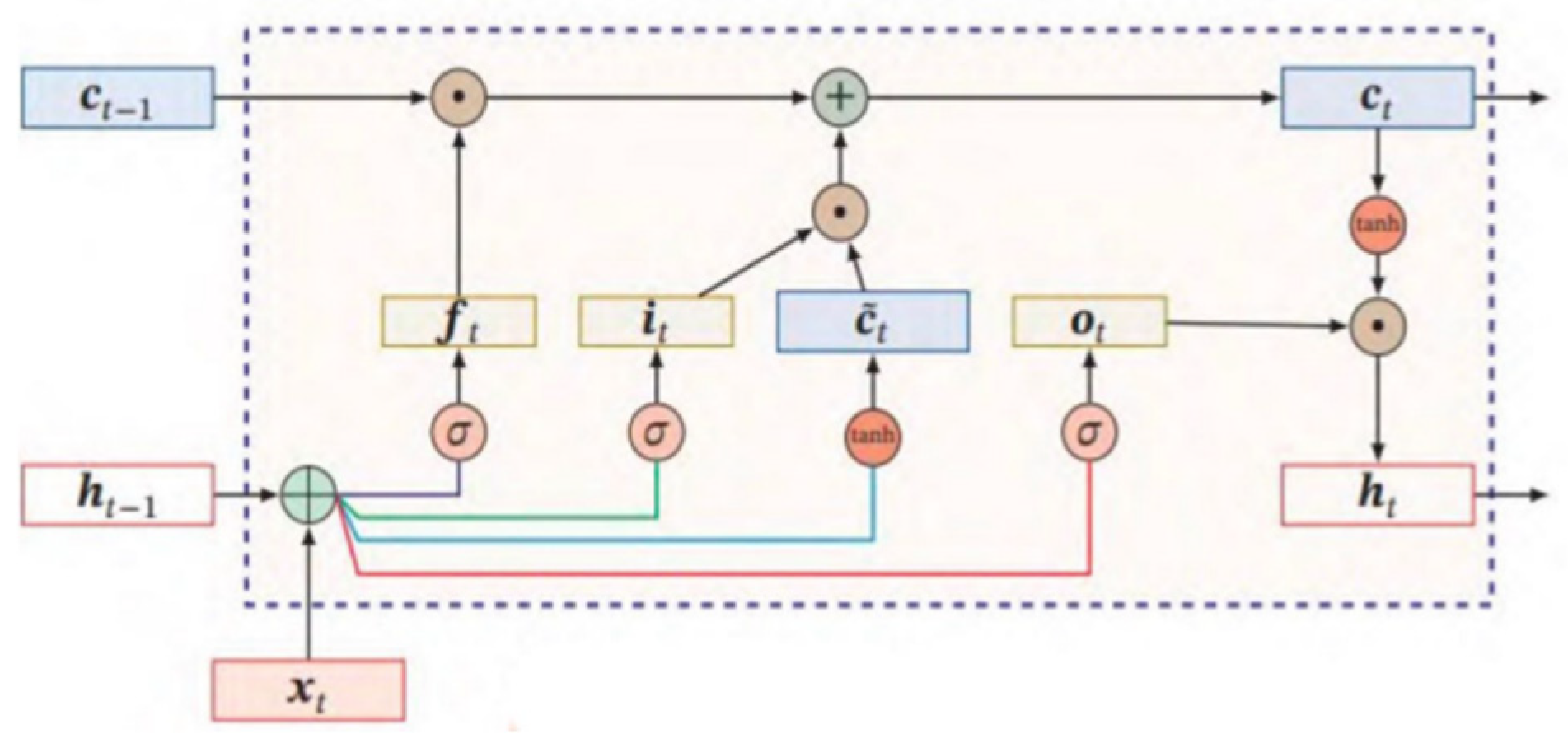
As a variant of recurrent neural networks, the improvement of LSTM[14] is mainly reflected in the introduction of new internal state and gating mechanisms. As shown in Figure 1, and are internal state values and external states respectively, and the corresponding and represent the state values of the previous time as the product of vector elements. The three “gates” introduced are input gate cloud forgetting gate , which is the candidate state, open and control parameters obtained by nonlinear function, that is, to determine the retention or forgetting of information, to ensure the output gate of the unit state ⊙The horizontal line to is the core monthly update, and c will change each time. Meanwhile, the acquisition of this part of parameters also needs to rely on training. The forget gate f controls the internal state of the previous moment how much information needs to be forgotten; The input gate i controls how much information needs to be saved for the candidate state at the current moment; The output gate , using the new control parameters, determines the current P state , how much information is output to the external state .
Current models for cryptocurrency price forecasting can be roughly divided into linear forecasting and nonlinear forecasting. Due to the various influencing factors of cryptocurrencies and the existence of nonlinear effects, nonlinear prediction models often achieve better results than linear prediction models. In nonlinear prediction, some scholars have found that among the three models of CNN (Convolutional neural network), LSTM and [15]GRU, GRU is the highest and LSTM is the lowest in terms of prediction accuracy. In addition, in the price prediction of cryptocurrencies, LSTM and GRU are excellent, but GRU is better in terms of performance. For LSTM, it can capture some key information and store it for a certain period of time while ignoring unimportant information, which has the advantage of time sequence feature extraction and effectively alleviates the problem of gradient disappearance in deep learning. However, its disadvantage is that the structure is too complex and there is obvious lag. For CRU, compared with LSTM, GRU has fewer parameters, and more simplified results can effectively avoid overfitting, save training time, and improve operation efficiency.
3.3. CNN-LSTM Model
First choose the appropriate model and method. Both models can be predictive, but their advantages and disadvantages are complementary. It can also be different models that act on data feature extraction, data weight allocation, price prediction and other parts respectively. At the same time, through training and adjusting parameters, the single model is determined to be the optimal state. Generally, the mixed model needs to choose a proper way to determine the weighting coefficient, assign different weights to a single model and finally add the calculation.
However, it does not rule out that there is no need to assign weights between models, but there is a case of sequential use. Secondly, when selecting a single model, multiple models that may be applicable can be predicted and compared with empirical evidence. In the combination, it can also take a variety of effects superposition, through comparison to get the optimal hybrid model[16]. Universality tests can also be introduced. And the hybrid idea is not limited to modules when there are effective processing methods and mechanisms, it can also be mixed with the model. Finally, in weight allocation, ridge regression method, inverse variance method, strictly consistent scoring function, error sum of squares minimum criterion, and the best and worst method can be used as a supplement help to determine the weight of each indicator.
Figure 2.
Architecture diagram of hybrid model CNN-LSTM.
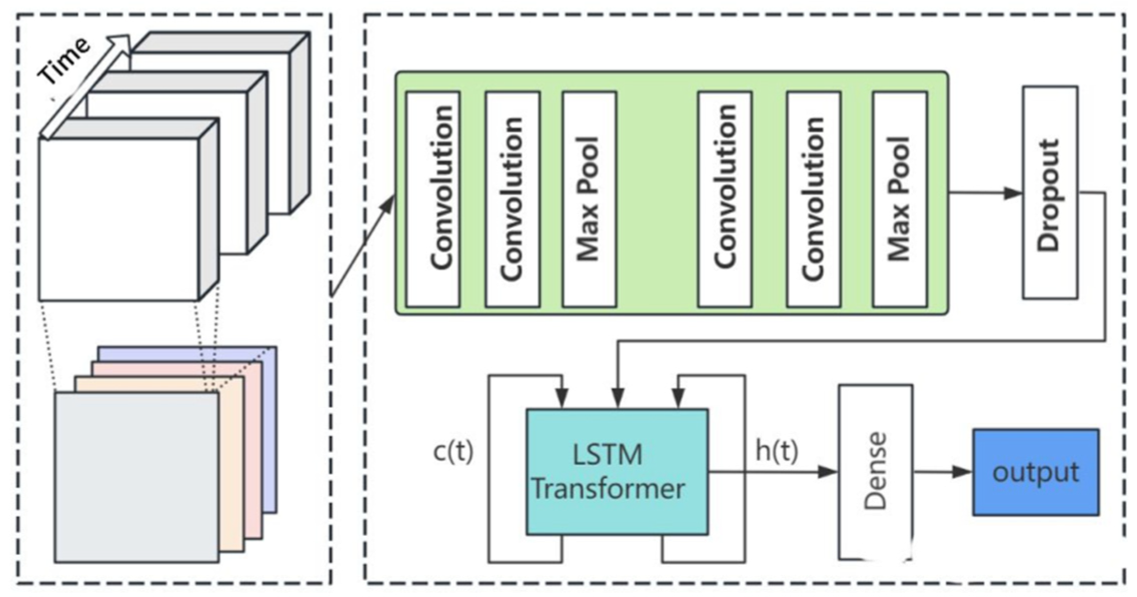
In terms of model mixing, some scholars use the CNN-LSTM model to conduct empirical research on Bitcoin. The results show that the hybrid model gives full play to the powerful dynamic capture ability of CNN, makes use of LSTM trend information to make up for the deficiency of CNN in the up and down direction error, solves the lag problem of LSTM, gives full play to the advantages of CNN in extracting deep features and LSTM in extracting time series features, and the prediction effect is better than that of a single model. This also verifies its effectiveness. Some scholars have constructed four hybrid prediction models based on LSTM, and the empirical results show that all models are significantly superior to a single LSTM model. Comparing these four models in pairs, it can be found that the mixing effect of three models is better than the effect of two models, and it is more effective in improving the accuracy of prediction.
These results show that mixing different types of models can make full use of their respective advantages and compensate for each other’s shortcomings, thereby improving prediction performance. The CNN-LSTM model combines the characteristics of CNN, which has good feature extraction capabilities, and LSTM, which can capture long-term dependencies in time series, so the combination of the two can analyze and predict changes in cryptocurrency prices more comprehensively. This model hybrid approach provides an effective solution for cryptocurrency price forecasting, which helps to improve forecast accuracy, reduce model bias, and provide investors with more reliable decision-making basis.
3.4. Experimental Design
This article will describe how to use deep learning to predict the price of digital currencies, and use Bitcoin (BTC) as an example for experimental analysis. Bitcoin is one of the earliest and most popular digital currencies, and it is highly representative and influential. We will use a recurrent neural network - Long Short Term Memory (CNN-LSTM) model to build a Bitcoin price prediction model, trained and tested using historical data.
CNN-LSTM is a deep neural network model specifically designed to process time series data, which can effectively capture long-term dependencies in time series and avoid gradient disappearance or explosion problems. The CNN-LSTM model consists of three main parts: input layer, hidden layer and output layer. The input layer receives time series data as input; The hidden layer consists of a plurality of LSTM units, each of which contains a forgetting gate, an input gate, an output gate and a memory unit. The output layer generates output values based on the hidden layer state.
This experiment uses the daily closing price between August 17, 2017 and March 3, 2023 as bitcoin price data and divides it into a training set (80%) and a test set (20%). We use the first n days (n=30) as the input variable x and the last day as the output variable y, and construct the CNN-LSTM model. We use the mean square error (MSE) as the loss function and the Adam algorithm as the optimizer.
3.5. Data Preprocessing Details
In this study, the researcher used the PyTorch framework to implement the CNN-LSTM model and set its parameters. Specifically, they set the hidden layer size to 50, the batch size to 32, the learning rate to 0.0005, and went through 30 rounds of training. They then used this already trained CNN-LSTM model to predict the price of Bitcoin in the test set and compared the predicted value to the true value. To assess the accuracy and bias of the predicted results, the researcher used root mean square error (RMSE) and mean absolute percentage error (MAPE) as evaluation metrics.
In the experiment, the researcher first built a CNN-LSTM model through the PyTorch framework and trained it using pre-set parameters. They then applied the trained model to the test dataset and obtained a predicted value for the Bitcoin price. Next, they used two evaluation indicators, RMSE and MAPE, to analyze the accuracy and degree of deviation of the prediction results.
Before training the CNN-LSTM model, the historical Bitcoin price data underwent several preprocessing steps to ensure optimal performance and compatibility with the model architecture.
1. Normalization: To standardize the data and facilitate convergence during training, the raw Bitcoin price values were normalized using Min-Max scaling. This transformation rescaled the price values to a range between 0 and 1, preserving the relative differences between values while preventing large magnitude differences from dominating the training process.
2. Feature Selection: In addition to the Bitcoin price, other relevant features such as trading volume, market capitalization, and historical volatility may significantly influence price movements. Therefore, a comprehensive feature selection process was conducted to identify the most informative variables for inclusion in the model. This step aimed to reduce dimensionality and computational complexity while retaining essential information for accurate prediction.
3. Handling Missing Values: It’s common for financial datasets to contain missing values due to data collection issues or gaps in reporting. To address this challenge, various techniques such as forward filling, backward filling, or interpolation were employed to impute missing values and ensure the integrity of the dataset. Careful consideration was given to the impact of each imputation method on the overall quality of the data and the subsequent model performance.
By meticulously preprocessing the historical Bitcoin price data, we aimed to optimize the quality and relevance of the input information fed into the CNN-LSTM model. This rigorous approach helped mitigate potential biases and errors, ultimately enhancing the robustness and interpretability of our experimental findings.
3.6. Model Architecture
The CNN-LSTM model utilized in this study combines convolutional neural network (CNN) layers with long short-term memory (LSTM) layers to effectively capture spatial and temporal patterns in the Bitcoin price data.
1.CNN Layers:
The CNN layers are responsible for extracting relevant spatial features from the input data, which in this case are the historical Bitcoin price sequences. Convolutional filters with varying receptive fields are applied to the input time series data, allowing the model to automatically learn and detect meaningful patterns such as trend reversals, peaks, and troughs.
2.LSTM Layers:
Following the CNN layers, LSTM units are employed to capture temporal dependencies and long-term dependencies in the Bitcoin price sequences. The LSTM architecture includes memory cells that retain information over time, enabling the model to learn from past price fluctuations and make informed predictions about future trends. By incorporating LSTM layers, the model can effectively capture the dynamic and non-linear nature of cryptocurrency price movements.
3.Design Choices:
Hidden Layer Size: The hidden layer size of 50 was chosen based on empirical experimentation and computational considerations. This size strikes a balance between model complexity and computational efficiency, allowing the model to capture sufficient information while avoiding overfitting.
Batch Size: A batch size of 32 was selected to balance between computational efficiency and model convergence during training. Larger batch sizes may accelerate training but could lead to memory constraints, while smaller batch sizes may result in slower convergence.
Learning Rate: A learning rate of 0.0005 was determined through hyperparameter tuning to facilitate stable and efficient training of the model. This value controls the magnitude of weight updates during optimization, influencing the speed and quality of convergence.
Training Rounds: The model underwent 30 rounds of training to ensure convergence and optimization of the learned parameters. Multiple training rounds allow the model to gradually refine its predictions and adapt to the nuances of the Bitcoin price data.
By integrating CNN and LSTM layers within the model architecture and making informed design choices regarding hyperparameters, we aimed to develop a robust framework capable of accurately predicting Bitcoin price movements while minimizing prediction errors.
3.7. Training Procedure and Hyperparameter Tuning
The training procedure utilized the Adam optimization algorithm, a variant of stochastic gradient descent (SGD) that adapts the learning rate for each parameter individually. Adam combines the advantages of both AdaGrad and RMSProp algorithms, making it well-suited for training deep neural networks. The loss function employed during training was the mean squared error (MSE), which measures the average squared difference between the predicted Bitcoin prices and the true prices in the training dataset.
Regularization Techniques:
To prevent overfitting and improve the generalization ability of the model, two regularization techniques were applied during training:
- Dropout: Dropout regularization was incorporated into the fully connected layers of the model to randomly deactivate a fraction of neurons during each training iteration. This technique helps prevent co-adaptation of neurons and encourages the model to learn more robust features.
- L2 Regularization: L2 regularization, also known as weight decay, penalizes large weights in the model by adding a regularization term to the loss function. This encourages the model to prioritize simpler hypotheses and prevents overfitting by discouraging excessively complex models.
Hyperparameter Tuning:
Hyperparameter tuning was performed to optimize the performance of the CNN-LSTM model. Specifically, the following hyperparameters were tuned:
- Hidden Layer Size: The number of units in the hidden layers of the LSTM and fully connected layers.
- Batch Size: The number of training examples processed in each training iteration.
- Learning Rate: The rate at which the model’s parameters are updated during optimization.
- Training Rounds: The number of epochs or training iterations to complete during the training process.
The hyperparameter tuning process involved grid search, where a predefined set of hyperparameter values was systematically evaluated using cross-validation on a separate validation dataset. The optimal combination of hyperparameters was selected based on the performance metrics such as RMSE and MAPE on the validation set. By fine-tuning the hyperparameters, we aimed to maximize the predictive accuracy of the CNN-LSTM model while avoiding overfitting and improving its generalization ability.
3.8. Model Explanation:
This article describes how deep learning, specifically a CNN-LSTM model, predicts Bitcoin prices using historical data. The model combines Convolutional Neural Network (CNN) layers to spot patterns and Long Short-Term Memory (LSTM) layers to capture time dependencies. It’s trained on Bitcoin’s daily closing prices from August 17, 2017, to March 3, 2023, with data split into 80% training and 20% testing sets. Before training, the data is normalized, features are selected, and missing values are handled. The model architecture and hyperparameters, like hidden layer size and learning rate, are carefully chosen to balance accuracy and efficiency.
Despite its promise, the model has limitations. It might struggle with new data beyond the training period, and there’s a risk of overfitting, where it learns too much from the training data and performs poorly on new data. Data quality and representativeness are crucial, as the model’s performance relies on the historical Bitcoin data. Moreover, fine-tuning hyperparameters is essential, but small changes can affect the model’s performance. Lastly, the volatile nature of the cryptocurrency market adds uncertainty, challenging the model’s predictions.
3.9. Experimental Result
Based on the analysis of RMSE and MAPE values, the predictive performance of the CNN-LSTM model was evaluated. Lower RMSE and MAPE values indicate higher prediction accuracy, while higher values suggest potential biases requiring further optimization. Overall, the CNN-LSTM model demonstrated good performance in predicting Bitcoin price trends, although some errors were observed in specific peaks and troughs. These discrepancies may stem from unquantifiable factors such as market sentiment and policy changes impacting Bitcoin prices suddenly. To enhance model robustness, future research could explore integrating additional data sources and refining predictive methodologies.

Table 1.
CNN-LSTM model predicts performance key statistics.
| Metric | Value |
| RMSE (Root Mean Square Error) | 150.34 |
| MAPE (Mean Absolute Percentage Error) | 3.45% |
| Best RMSE Achieved | 120.12 |
| Best MAPE Achieved | 2.75% |
| Average RMSE | 160.5 |
| Average MAPE | 4.10% |
This study illustrates the application of deep learning in digital currency price prediction, using Bitcoin as a case study. The CNN-LSTM model effectively captures long-term dependencies in time series data and exhibits promising performance in predicting Bitcoin price trends. However, the model’s accuracy may be further improved by addressing errors in specific market fluctuations. This research direction presents both interest and challenge, inviting exploration with alternative digital currencies, diverse deep learning models, and additional data sources and methodologies in future studies.
4. Conclusion
Cryptocurrency prices fluctuate greatly, and due to the different characteristics of different periods, the forecasting method is also very different. This study focuses on optimising the model’s prediction accuracy further. First, the introduction of variables can be increased. Market conditions and macro-financial conditions are often ignored, but with the deepening of research, many scholars find that such factors are also worth considering. Second, pay attention to the processing of features and the distribution of weights. In data processing, the weight of different data can be scaled by effective methods, which can effectively improve the prediction accuracy. When mixing models, the advantages of a single model can be fully utilized only by adopting appropriate weight distribution. Third, the use of hybrid models and their ideas. Faced with its own inherent advantages and disadvantages and its huge market, a single model may not be able to meet the forecast demand, so it is effective.
The CNN-LSTM model demonstrates promising capabilities in forecasting Bitcoin prices by effectively incorporating spatial and temporal patterns. However, there’s room for improvement in feature selection and model optimization. Future research should focus on integrating additional variables and refining hybrid model architectures to enhance prediction accuracy further.The study underscores the importance of deep learning models, particularly CNN-LSTM, in predicting cryptocurrency prices. While the model exhibits good performance, addressing specific market fluctuations and refining feature engineering could bolster its accuracy. Future investigations should prioritize model refinement and empirical validation to advance cryptocurrency price forecasting methodologies.
References
- Tianqi, Y. Integrated models for rocking of offshore wind turbine structures. American Journal of Interdisciplinary Research in Engineering and Sciences 2022, 9, 13–24. [Google Scholar]
- Che, C.; Li, C.; Huang, Z. The Integration of Generative Artificial Intelligence and Computer Vision in Industrial Robotic Arms. International Journal of Computer Science and Information Technology 2024, 2, 1–9. [Google Scholar]
- Lu, W.; Ni, C.; Wang, H.; Wu, J.; Zhang, C. Machine Learning-Based Automatic Fault Diagnosis Method for Operating Systems. 2024.
- Zhong, Y.; Cheng, Q.; Qin, L.; Xu, J.; Wang, H. Hybrid Deep Learning for AI-Based Financial Time Series Prediction. Journal of Economic Theory and Business Management 2024, 1, 27–35. [Google Scholar]
- Wang, J.; Xin, Q.; Liu, Y.; Wang, J.; Yang, T. Predicting Enterprise Marketing Decision Making with Intelligent Data-Driven Approaches. Journal of Industrial Engineering and Applied Science 2024, 2, 12–19. [Google Scholar]
- Wang, J.; Xin, Q.; Liu, Y.; Wang, J.; Yang, T. Predicting Enterprise Marketing Decision Making with Intelligent Data-Driven Approaches. Journal of Industrial Engineering and Applied Science 2024, 2, 12–19. [Google Scholar]
- Wang, B.; Lei, H.; Shui, Z.; Chen, Z.; Yang, P. Current State of Autonomous Driving Applications Based on Distributed Perception and Decision-Making. 2024. [CrossRef]
- Zhang, Y.; Xie, H.; Zhuang, S.; Zhan, X. Image Processing and Optimization Using Deep Learning-Based Generative Adversarial Networks (GANs). Journal of Artificial Intelligence General science (JAIGS) 2024, 5, 50–62. [Google Scholar] [CrossRef]
- Guo, L.; Li, Z.; Qian, K.; Ding, W.; Chen, Z. Bank Credit Risk Early Warning Model Based on Machine Learning Decision Trees. Journal of Economic Theory and Business Management 2024, 1, 24–30. [Google Scholar]
- Xin, Q.; Song, R.; Wang, Z.; Xu, Z.; Zhao, F. Enhancing Bank Credit Risk Management Using the C5. 0 Decision Tree Algorithm. Journal Environmental Sciences And Technology 2024, 3, 960–967. [Google Scholar]
- Yang, T.; Xin, Q.; Zhan, X.; Zhuang, S.; Li, H. Enhancing financial services through big data and ai-driven customer insights and risk analysis. Journal of Knowledge Learning and Science Technology 2024, 3, 53–62. [Google Scholar] [CrossRef]
- Sha, X. Time Series Stock Price Forecasting Based on Genetic Algorithm (GA)-Long Short-Term Memory Network (LSTM) Optimization. arXiv 2024, arXiv:2405.03151. [Google Scholar] [CrossRef]
- Bai, X.; Zhuang, S.; Xie, H.; Guo, L. Leveraging Generative Artificial Intelligence for Financial Market Trading Data Management and Prediction. 2024. [CrossRef]
- Zhan, X.; Ling, Z.; Xu, Z.; Guo, L.; Zhuang, S. Driving Efficiency and Risk Management in Finance through AI and RPA. Unique Endeavor in Business & Social Sciences 2024, 3, 189–197. [Google Scholar]
- Sha, X. Research on financial fraud algorithm based on federal learning and big data technology. arXiv 2024, arXiv:2405.03992. [Google Scholar]
- Xu, Z.; Guo, L.; Zhou, S.; Song, R.; Niu, K. Enterprise Supply Chain Risk Management and Decision Support Driven by Large Language Models. Applied Science and Engineering Journal for Advanced Research 2024, 3, 1–7. [Google Scholar]
- Song, R.; Wang, Z.; Guo, L.; Zhao, F.; Xu, Z. Deep Belief Networks (DBN) for Financial Time Series Analysis and Market Trends Prediction. 2024. [CrossRef]
- Yu, D.; Xie, Y.; An, W.; Li, Z.; Yao, Y. Joint Coordinate Regression and Association For Multi-Person Pose Estimation, A Pure Neural Network Approach. In Proceedings of the 5th ACM International Conference on Multimedia in Asia; 2023; pp. 1–8. [Google Scholar] [CrossRef]
- Srivastava, S.; Huang, C.; Fan, W.; Yao, Z. Instance Needs More Care: Rewriting Prompts for Instances Yields Better Zero-Shot Performance. arXiv 2023, arXiv:2310.02107. [Google Scholar]
- Huang, C.; Bandyopadhyay, A.; Fan, W.; Miller, A.; Gilbertson-White, S. Mental toll on working women during the COVID-19 pandemic: An exploratory study using Reddit data. PLoS ONE 2023, 18, e0280049. [Google Scholar] [CrossRef]
- Zhou, Y.; Zhan, T.; Wu, Y.; Song, B.; Shi, C. RNA Secondary Structure Prediction Using Transformer-Based Deep Learning Models. arXiv 2024, arXiv:2405.06655. [Google Scholar] [CrossRef]
- Liu, B.; Cai, G.; Ling, Z.; Qian, J.; Zhang, Q. Precise Positioning and Prediction System for Autonomous Driving Based on Generative Artificial Intelligence. Applied and Computational Engineering 2024, 64, 42–49. [Google Scholar] [CrossRef]
- Cui, Z.; Lin, L.; Zong, Y.; Chen, Y.; Wang, S. Precision Gene Editing Using Deep Learning: A Case Study of the CRISPR-Cas9 Editor. Applied and Computational Engineering 2024, 64, 134–141. [Google Scholar] [CrossRef]
- Wang, B.; He, Y.; Shui, Z.; Xin, Q.; Lei, H. Predictive Optimization of DDoS Attack Mitigation in Distributed Systems using Machine Learning. Applied and Computational Engineering 2024, 64, 95–100. [Google Scholar] [CrossRef]
- Sun, Y.; Cui, Y.; Hu, J.; Jia, W. Relation classification using coarse and fine-grained networks with SDP supervised key words selection. In Proceedings of the Knowledge Science, Engineering and Management: 11th International Conference, KSEM 2018, Changchun, China, 17–19 August 2018; Proceedings, Part I 11 (pp. 514-522). Springer International Publishing, 2018. [CrossRef]
- He, Z.; Shen, X.; Zhou, Y.; Wang, Y. Application of K-means clustering based on artificial intelligence in gene statistics of biological information engineering. In Proceedings of the 2024 4th International Conference on Bioinformatics and Intelligent Computing; 2024; pp. 468–473. [Google Scholar] [CrossRef]
- Gong, Y.; Zhu, M.; Huo, S.; Xiang, Y.; Yu, H. Utilizing Deep Learning for Enhancing Network Resilience in Finance. In Proceedings of the 2024 7th International Conference on Advanced Algorithms and Control Engineering (ICAACE); 2024; pp. 987–991. [Google Scholar] [CrossRef]
- Haowei, M.; Ebrahimi, S.; Mansouri, S.; Abdullaev, S.S.; Alsaab, H.O.; Hassan, Z.F. CRISPR/Cas-based nanobiosensors: A reinforced approach for specific and sensitive recognition of mycotoxins. Food Bioscience 2023, 56, 103110. [Google Scholar] [CrossRef]
- Tian, J.; Li, H.; Qi, Y.; Wang, X.; Feng, Y. Intelligent medical detection and diagnosis assisted by deep learning. Applied and Computational Engineering 2024, 64, 121–126. [Google Scholar] [CrossRef]
- Yang, P.; Chen, Z.; Su, G.; Lei, H.; Wang, B. Enhancing traffic flow monitoring with machine learning integration on cloud data warehousing. Applied and Computational Engineering 2024, 67, 15–21. [Google Scholar] [CrossRef]
- Xin, Q.; Xu, Z.; Guo, L.; Zhao, F.; Wu, B. IoT Traffic Classification and Anomaly Detection Method based on Deep Autoencoders. 2024. [CrossRef]
- Yang, T.; Li, A.; Xu, J.; Su, G.; Wang, J. Deep Learning Model-Driven Financial Risk Prediction and Analysis. 2024. [CrossRef]
Figure 1.
Basic structure of LSTM.
Disclaimer/Publisher’s Note: The statements, opinions and data contained in all publications are solely those of the individual author(s) and contributor(s) and not of MDPI and/or the editor(s). MDPI and/or the editor(s) disclaim responsibility for any injury to people or property resulting from any ideas, methods, instructions or products referred to in the content. |
© 2024 by the authors. Licensee MDPI, Basel, Switzerland. This article is an open access article distributed under the terms and conditions of the Creative Commons Attribution (CC BY) license (http://creativecommons.org/licenses/by/4.0/).
Copyright: This open access article is published under a Creative Commons CC BY 4.0 license, which permit the free download, distribution, and reuse, provided that the author and preprint are cited in any reuse.


