
Submitted:
04 March 2025
Posted:
05 March 2025
You are already at the latest version
Abstract
The cryptocurrency market is currently one of the most interesting areas for investment, attracting both experienced and casual investors. Although it can offer high returns, it also poses significant risks due to its high volatility. In this context, artificial intelligence, particularly through deep learning and machine learning algorithms, has played a key role in developing applications that provide investment advice, with the aim of maximizing returns and reducing investment risks.
This study proposes a system for forecasting the closing prices of ten of the leading cryptocurrencies currently available in the market, presented in a web application capable of making predictions ranging from one to four hours. To achieve this, different models using various machine learning and deep learning algorithms were analyzed and tested, including Recurrent Neural Networks, time series analysis algorithms such as ARIMA, and even some more conventional regression algorithms. For algorithm comparison, minute step Bitcoin price data over a 30-day period was used to forecast prices 60 minutes ahead. Through extensive experimentation, the GRU neural network demonstrated superior predictive accuracy, achieving MAPE = 0.09\%, MSE = 5954.89, RMSE = 77.17, and MAE = 60.20. A web application was also developed, which integrates the best-performing model to provide real-time price predictions for multiple cryptocurrencies.
Keywords:
Forecasting
; Cryptocurrency
; Machine Learning
; Time Series
1. Introduction
Cryptocurrencies currently constitute a highly attractive investment market, but they come with a high risk due to their extreme volatility. Cryptocurrencies are not subject to the same regulations as stock exchanges or banking institutions, nor do they adhere to their rules. They are a global, decentralized digital capital that allows for worldwide fund transfers in seconds without prior oversight. Investors face the question of "where to invest?" due to the large number of cryptocurrencies available on the market, with new assets emerging every day and others disappearing. Some cryptocurrencies have a more consistent track record, but the one with the most relevance and that started this whole revolution is Bitcoin, which was launched in 2008 [1].
Cryptocurrency price fluctuations occur every minute, 24 hours a day. Therefore, experts must be constantly alert to changes and well informed to generate market indicators. In this context, computer systems based on artificial intelligence have emerged, acting as decision support systems, using machine learning algorithms to make future projections based on historical data [2]. This type of data analysis indexed over time is called time series analysis.
Cryptocurrency price values represent a non-stationary time series, meaning that the observed patterns are not constant over time and therefore will not necessarily recur in the future. This makes the challenge of developing a machine learning model capable of producing reliable projections a rather difficult task to achieve.
In addition to time-series analysis, there is a wide range of models that can be implemented using various machine learning techniques, regression models, and even deep learning models. The results will depend on the quantity and quality of available data, the attributes used for the training, and the type of forecast desired. Although existing machine learning models are not difficult to implement, they may require significant computational resources depending on the size of the records and attributes used in the training process. If the number of attributes can affect performance, the selection of these attributes for the learning process also affects the results. Therefore, a careful selection of attributes that can refine projections is necessary. More information or a higher number of "attributes" does not always result in better models [3].
Another factor that can impact results is the time horizon of the data. The behaviors observed five or ten years ago may not reflect current patterns. However, a very short time horizon may result in insufficient data for reliable model forecasts [3].
The results of the machine learning models will also depend on the type of projection desired. That is, whether one aims to predict an appreciation or depreciation in the next minute, hour, day, or following days, or to forecast the price value in the next minute, hour, day, or days.
The main objective of this work is to analyze the performance of different machine learning models for cryptocurrency price prediction and to develop an application that uses the most capable machine learning model to make future projections of different cryptocurrencies at a high-frequency level, i.e., using minute-step data, using different forecast time horizons ranging from one to four hours. For this purpose, ten of the main cryptocurrencies currently on the market were selected, specifically Bitcoin, Ethereum, Binance Coin, Cardano, Solana, XRP, Polkadot, USD Coin, Dogecoin and Avalanche. This selection was based on information provided by one of the main reference platforms, coinmarketcap.com, which offers real-time cryptocurrency quotes.
This paper organizes the remaining sections as follows: Section 2 reviews prior research on cryptocurrency price prediction. The next section will detail the entire work methodology, which includes data acquisition, data preparation, developed prediction models, and their evaluation. In the next section, the results are discussed. Section 5 deals with the model deployment and describes the web application that was developed. The final section discloses the main conclusions and prospects for future work.
2. State of the Art
For the literature review, only scientific papers from the Springer and IEEE databases were looked at. The keywords cryptocurrency, machine learning, and forecasting were used. In total, 56 papers were found.
2.1. Bitcoin
Bitcoin is the first and most significant cryptocurrency on the market, being the most relevant among the selected for this study. Bitcoin was introduced in 2008 by an anonymous group under the pseudonym Satoshi Nakamoto and became operational in 2009 as an open-source network for peer-to-peer digital transactions [1]. It paved the way for Blockchain technology, which ensures transaction security through advanced cryptography. Its success led to the creation of other cryptocurrencies, and by 2021, the cryptocurrency market capitalization surpassed $1.5 trillion USD [4].
Bitcoin and other cryptocurrencies are considered speculative assets, with idiosyncratic prices driven by behavioral factors, not correlated with major financial assets. This attracted the interest of fund managers and researchers, especially in the use of machine learning algorithms for trading [5].
Bitcoin transactions are recorded in a public database (Blockchain) and verified by miners, who are rewarded with newly created Bitcoins. Unlike traditional systems, Bitcoin transactions are irreversible, reducing fraud, while the system provides high liquidity, low costs, and fast transactions [6].
Therefore, the Bitcoin ecosystem includes characteristics such as being immaterial, decentralized, accessible, transparent, economical, and irreversible, with fast and secure transactions. The currency is divisible (with the smallest unit being the satoshi) and resistant to attacks, with a total supply limited at 21 million units [5].
2.2. Time Series
Time series forecasting problems are challenging due to many unpredictable factors, resulting in complex temporal dependencies. Time series are present in various real-world applications, such as commercial transactions, econometrics, and finance [7].
These data consist of a sequence of discrete points obtained at regular time intervals. The main difference between time series and other types of data is that their characteristics must remain invariant over time. However, many real-world time series are non-stationary, meaning that properties such as mean and variance change over time, leading to high volatility and trend [7].
Time series forecasts can be univariate, using only past values of a single dependent variable, or multivariate, when N features are correlated with each other. In the case of cryptocurrencies, these features include opening, closing, high, low prices, and the traded volume within a given time interval [4].
2.3. Related Work
The works presented in this section are only those that focus on forecasting the future behavior of cryptocurrencies using machine learning models. Other studies could also be added, particularly those on predicting stock market behaviors, real estate markets, and other assets that also use machine learning models. This is especially relevant because some articles, such as [7] and [8], among others, use different objects for prediction beyond cryptocurrencies. However, cryptocurrencies exhibit distinct characteristics that result in different behaviors due to their decentralized nature, as there is no global organism for their regulation.
From the research conducted, which includes a total of 56 articles, it is clear that the most studied cryptocurrency is Bitcoin, as it is the most relevant cryptocurrency with the largest market share. As shown in Figure 1, out of the 56 articles analyzed, 26 use only Bitcoin as the prediction object, 21 use Bitcoin alongside other assets or cryptocurrencies, and only 9 use other cryptocurrencies besides Bitcoin, including Ethereum, the second most relevant cryptocurrency in the market.
Another observed aspect relates to the type of forecasting that is performed, whether it’s price prediction using regression models or signal classification (positive or negative), indicating whether the value will rise or fall. The classification can also take the form of instructions or recommendations, such as Hold/Buy/Sell, as in [9], functioning as a decision support system. Other types of forecasts found include profitability rates and volatility predictions.
The forecasting time horizon varies widely, ranging from minutes, hours, days, weeks, or even months. In the cryptocurrency market, thousands of transactions are made every second, 24 hours a day, seven days a week, with prices fluctuating by the second.
The vast majority of articles, 47, focus on price predictions, 4 on signal classification, and the remaining 7 perform other types of forecasting, as shown in Figure 2. In this case, as in others that will be presented, the total does not sum to 56 because some articles, such as [10], use more than one type of forecast type.
Another relevant aspect of the analyzed studies is the predictor attributes used in the developed models:
13 articles present models that use only the cryptocurrency price or quotation, this price being the close price of the time interval (timestep) in the dataset used. This time interval in the datasets can range from seconds, minutes, hours, to days. 18 articles only use the most common attributes, which are typically provided in market quotation datasets, namely Open, High, Low, Close, and Volume. These correspond to the opening price of the interval, the highest price traded in the interval, the lowest price traded in the interval, the final price of the interval, and the volume traded in the interval, respectively. In addition to those previously mentioned, 14 studies use other attributes or indicators for their forecasting models; 4 use quotations from different cryptocurrencies or other assets; and 9 articles use text-based attributes. These text attributes reflect sentiment analysis, positive or negative, regarding the cryptocurrency or object of analysis. Sentiment analysis is conducted on headlines and news articles, or social media posts and comments, such as on Twitter. Figure 3 shows the distribution of the types of attributes used in the analyzed studies.
Another relevant aspect that may also influence the performance of the models is the time periods of the datasets. It is not guaranteed that a model that performs well in one specific period will have the same performance in another distinct period. This is an aspect that varies significantly and is almost unique to each article. The periods covered, the time horizon, and the interval of the records (seconds, minutes, hours, days) all vary. Articles such as [2] use a dataset that spans 8 years, or [11], which uses a 7 months range, with some articles using either broader or more restricted periods.
In general, the distribution of the periods used is as shown in the graph in Figure 4, where it can be seen that the year with the greatest presence in the datasets is 2018, and only 5 articles use datasets that include the year 2022, even though 30 of the 56 articles were already published in 2022/2023. This can be explained by the time required for data collection, processing, model development, and testing, in addition to the writing of the respective articles.
From the analysis of the related works, the machine learning models used can also be highlighted, with the LSTM model being the most used, appearing in 26 articles. SVM (or SVR) is the second most used, appearing in 20 articles, and Random Forest completes the top 3 with 15 articles. The ARIMA model, the most common for time series forecasting, is found in 10 articles. Other models that also stand out with good performances are the GRU Recurrent Neural Networks, with 11 articles, and models such as Gradient Boosting/Extreme Gradient Boosting, present in 12 articles. Other models used in the studies include Facebook Prophet, ELM (Extreme Learning Machine), and LASSO (Least Absolute Shrinkage and Selection Operator). These models are not emphasized because they are used less often in this way of thinking and do not produce standout results. Figure 5 shows the distribution of these models.
Lastly, it is necessary to highlight the metrics used to evaluate the performance of the models. Among these metrics, RMSE, MAPE, MAE, MSE, and stand out as regression metrics, while F1 Score and Accuracy are used as classification metrics.
From the analysis of Figure 6, it is clear that error metrics are more common than classification metrics.
There are frequently comparison graphs between the actual values and the values predicted by the models. However, comparing the articles is somehow difficult to achieve, as they do not use the same metrics, and the objects of study (cryptocurrencies) are not the same, nor are the time periods used in the training and testing datasets. It is impossible to ensure that the results would hold using a different cryptocurrency and a different dataset.
The metric values vary significantly between the articles. The values found show the variations presented in Table 1 based on the best performance.
3. Model Development and Evaluation
The models were developed in Python, a simple and widely used programming language for developing software that use machine learning libraries. Additionally, there is a vast amount of information and code examples available for reference.
3.1. Datasets
For the training and testing of the models, different datasets were collected, which include the minute step price values of Bitcoin, Ethereum, Binance Coin, Cardano, Solana, XRP, Polkadot, USD Coin, Dogecoin, and Avalanche. The data was obtained using the Python library YFinance, which allows the extraction of cryptocurrency prices as well as other financial assets, available on the portal finance.yahoo.com.
We collected data from 12/05/2024 to 11/06/2024 to train and test the models’ minute step price values over a 30-day period.
The records include the attributes Datetime, Open, High, Low, Close, Adj. Close, and Volume, corresponding to the date and time of the price, opening value of the period, highest value traded during the period, lowest value traded during the period, closing value of the period, adjusted closing value of the period, and volume traded during the period. These fields, or attributes, are common across all financial asset quotations, from cryptocurrencies to stock market or Forex prices.
As can be seen in Table 2 and Table 3, although the same function with the same parameters is used to retrieve the data, the number of records is not the same for all cryptocurrencies, varying between 31,670 for Polkadot and 38,216 for Ethereum.
All values are in USD, and the prices vary significantly depending on the cryptocurrency. The average value for Dogecoin is 0.16 USD, the cryptocurrency with the lowest price, while the average value for Bitcoin is 67,948.15 USD, the highest-priced cryptocurrency. In terms of trading volume per minute, Polkadot has the lowest average value, at 76,259.87 USD, while Bitcoin has the highest, at 8,879,468.76 USD. Figure 7 show the Closing Price for all cryptocurrencies across the collect data period.
3.2. Data Preparation
For the datasets obtained via the YFinance API, there is not much work required at this stage, as the data is retrieved in the same format for all cryptocurrencies and no null or empty values are passed. However, this verification is performed to ensure that no null values are passed for the training and testing of the models.
After being retrieved, the records are stored in a CSV file so they can be reused and processed throughout the modeling and testing process, ensuring that the data is the same for all models and that the results are not influenced by different data being used for different models.
The Datetime attribute is used as the index for the records, and its sorting is ensured so that the records are always sequential based on date and time.
The Adj. Close column is removed from all cryptocurrency datasets, as it contains the same values as the Close attribute and is therefore redundant.
With the exception of the SARIMA model, which only uses the Close attribute, the data is scaled using the MinMaxScaler function from the sklearn library to ensure that all attribute values are on the same scale for model training. This scale is then reversed for model testing and validation.
The tests and comparison of the models were based on the 60-minute forecast, and the data was divided as follows:
- The last 60 records are used for validation.
- 80% of the remaining records are used for training.
- 20% of the remaining records are used for testing.
3.3. Evaluation Metrics
After training the machine learning models, error metrics are calculated using the test dataset to evaluate the performance of regression models. The performance metrics measure how close the actual results are to the predicted values, with the most common ones being the Mean Absolute Error (MAE), Mean Squared Error (MSE), Root Mean Squared Error (RMSE), and Mean Absolute Percentage Error (MAPE) [12].
Where represents the actual value, and represents the value predicted by the model [13].
3.4. Models
First, we compare the performance of the eight different regression algorithms using the Bitcoin records for 60-minute forecasts. This choice is due to the fact that Bitcoin is the most relevant and commonly used cryptocurrency in the analyzed studies. We selected the 60-minute timeframe because it is the shortest time horizon under analysis, thereby ensuring optimal performance.
The comparative tests were based on the use of all attributes—Open, High, Low, Close, and Volume—as well as on just the Close attribute. The SARIMA model was only trained and tested using the Close attribute because it has some particularities that distinguish it from the other models, which will be explained next.
In general, the models can be used with data from different time intervals. The records are available through the YFinance API, which allows downloading records by the minute, hour, or day. For minute-level data, the last 30 days of data can be retrieved. For hourly intervals, data from the last 365 days can be retrieved, and for daily records, there are no restrictions.
The decision to use minute-level data allows for a much larger amount of records for model training. Some models, such as neural networks, require a large amount of data to achieve better performance. In 30 days, there can be up to 43,200 records, while in one year of hourly data, there can be up to 8,760, and in five years of daily records, there could only be up to 1,825 records.
Another relevant aspect of minute-step records is that the variation in values between records is less significant, which also helps to make predictions more accurate.
Except for the SARIMA model, where values are trained minute by minute, for all the other models, there is a function to create forecasts in 60-minute sequences, also known as sliding windows. This function is adjusted according to the forecast time horizon. Thus, the last 60 minutes are used to predict the next 60 minutes.
The model’s performance is measured using the metrics previously mentioned: MSE, RMSE, MAE, and MAPE. Additionally, the nRMSE metric is introduced, which corresponds to the RMSE metric but obtained from normalized values, allowing for better comparison of model performance across different cryptocurrencies, as each one has different magnitude values.
From Keras library of the TensorFlow API, the models Long Short-Term Memory (LSTM) [14] and Gated Recurrent Unit (GRU) [15] were used, and both models were tested with 50 neurons, two layers, Adam optimizer and the loss values were calculated based on MSE. These models run for 50 epochs, and can be stopped earlier using the EarlyStopping method if the loss function values begin to increase consecutively for 5 epochs. The GRU model, in terms of Python programming, is quite similar to the LSTM, however, it is a simpler and faster model, which can also be more efficient as it handles data overfitting better.
The Auto-Regressive Integrated Moving Average (ARIMA) [16] model is obtained through the Statsmodels library. The model used is actually SARIMAX, which is prepared to use seasonality and exogenous variables in the ARIMA model, but in this case, there are no exogenous variables in the data obtained, and for that reason, the model is referred to as SARIMA and not ARIMA nor SARIMAX. This model is very resource-intensive, and on the machine where it was tested, it was not even possible to load the entire dataset to train the model. Therefore, subsets of the records were loaded, and the point where the best results were achieved was with only 360 records, meaning the price of the last 360 minutes. Even so, the model takes a long time to train, which makes it impractical for deployment in an application, as it needs to be retrained with new data to make predictions, unlike the other models that can be saved and reused to make predictions with new data without requiring training the model again.
The Linear Regression [17] is the simplest regression model, and despite that its performance was quite interesting. What was observed with the previous models is that they can more or less follow the price trends, but they do not predict the major peaks in value variation. Linear Regression tends to be even more of a straight line when presented graphically. The main advantage is that it is a very simple and fast model to train.
The Random Forest [18] model is not very common for time series forecasting, and the training process is also quite heavy when used with a large amount of data. To avoid overloading the training process too much, a model with 100 decision trees was applied. The performance of this model was slightly worse than the previous models.
The Support Vector Machine (SVM) [19] model, Support Vector Regressor for regression problems, was tested with the kernel parameter set to RBF. This model is also heavy to train with large datasets, but it performs well, especially when trained with all attributes.
The XGBoost [20] model, in terms of training, is quite fast, however, its performance in validation fell well short of the previous models, especially when trained with all attributes. In the parameters, 100 decision trees, or predictors, were used, along with a learning rate of 0.1.
Lastly, LightGBM [21], a model derived from XGBoost, achieves better results with faster training. Using default configuration values, its performance, although not as good as neural networks, is better than XGBoost when used with all predictor attributes, but worse when used with only the closing price.
3.4.1. Analysis of Models Performance
Table 4 provides a performance comparison of the eight different machine learning models developed.
The GRU model with all attributes outperformed all other models across all metrics, achieving the lowest MSE (5,954.89), RMSE (77.17), MAE (60.20), and MAPE (0.09%). Its normalized RMSE (nRMSE) was also the lowest (0.19), highlighting its robustness in handling Bitcoin’s price fluctuations. The GRU’s performance slightly declined when using only the Close attribute, with an RMSE of 96.47 and a MAPE of 0.11%. This indicates that the model benefits from having access to a wider range of input features to improve prediction accuracy. The LSTM model performed competitively, coming in second after the GRU. With all attributes, it achieved an MSE of 8,163.73 and a MAPE of 0.11%. Similar to GRU, its performance dropped when only the Close attribute was used, with an MSE of 7,237.85 and a MAPE of 0.10%. The LSTM’s slightly higher computational complexity may explain its lower performance compared to GRU for this dataset. The SARIMA model, tested only with the Close attribute, showed significantly worse results compared to GRU and LSTM. With an RMSE of 139.56 and a MAPE of 0.16%, SARIMA struggled with the volatile nature of Bitcoin prices. This may be due to its reliance on linear assumptions and the inability to capture complex patterns in the data, unlike the neural network models. Surprisingly, Linear Regression performed relatively well considering its simplicity. With all attributes, it achieved an RMSE of 83.54 and a MAPE of 0.10%, making it a lightweight yet effective option for basic price forecasting. However, its inability to predict extreme price peaks and valleys limits its applicability in high-volatility markets like cryptocurrencies. The ensemble and decision tree-based models performed worse than both GRU and LSTM, especially when trained with all attributes. For instance, XGBoost had an RMSE of 2050.87 and a MAPE of 1.57%, highlighting its struggle to adapt to the intricate time-series patterns in cryptocurrency data. LightGBM, while faster to train than XGBoost, also had higher errors compared to the neural network models.
The superiority of the GRU model, as demonstrated by its consistently lower error metrics, can be attributed to its ability to effectively model sequential data with fewer computational resources than LSTM, without compromising accuracy. The GRU’s simplified architecture compared to LSTM allows for faster training times while still maintaining the ability to capture long-term dependencies, making it particularly useful for real-time applications like cryptocurrency forecasting. In contrast, traditional models like ARIMA and regression-based algorithms, while still useful for certain financial forecasting tasks, struggled to adapt to the rapidly fluctuating nature of cryptocurrency prices. This reinforces the need for models that can accommodate non-linear and non-stationary behaviors, characteristics intrinsic to cryptocurrencies. In conclusion, the GRU model is not only the most accurate model tested but also the most practical for deployment in real-time forecasting systems, where computational efficiency is critical. Its performance highlights the potential for deep learning models to provide accurate, short-term predictions in highly volatile markets like cryptocurrencies.
3.4.2. Time Horizons
It is observed that the performance significantly decreases as the forecast horizon increases when using high-frequency data, which was expected, as forecasting so many steps ahead is much more difficult. Especially when the model is unable to predict major drops or peaks in value, and cannot foresee changes in trend direction. In other words, if a cryptocurrency is in an upward trend, the model will make predictions in the same direction, and if there is a change in the trend, the model will not predict it, as there are no predictor attributes indicating such a change might occur.
In order to study the performance of the GRU network across different forecast time horizons, the GRU was configured to run up to 50 learning cycles (epochs); however, with the EarlyStopping method configured to tolerate 5 epochs if the loss function values start increasing, the process generally does not exceed 20 cycles in each training process.
Initially, shorter forecast horizons of 30, and 45 minutes were planned, but the performance did not improve enough to justify making them available in the web application. Longer horizons of 6, 12, and 24 hours were also considered, but here the performance dropped too much. Most likely, for these longer forecast horizons, the models would train better with hourly data instead of minute-level data.
4. Results Discussion
The GRU neural network, recognized as the most effective prediction method, was used to develop forecasting models for all selected cryptocurrencies throughout time horizons ranging from 60 to 240 minutes.
In terms of performance comparison between the different cryptocurrencies with varying magnitudes, the only comparable metrics are MAPE, which is a percentage metric, and nRMSE, which is a normalized RMSE value. As can be seen from Figure 9 and Table 6, an overall increase in forecast error values is observed from the 60-minute prediction to bigger time horizons, with the exception of USD Coin, which has such subtle price variations that it shows little difference across forecasts with different time horizons.
Except for USD Coin, the following observations stand out from the tests performed: Bitcoin achieved the best performance in terms of nRMSE across all four time horizons. Also, in terms of the nRMSE metric, the worst performances were with Avalanche at 60 minutes and with Dogecoin at 120, 180, and 240 minutes, along with XRP in the last case. In terms of MAPE values, Bitcoin and Cardano had the best performance at 60 minutes, Binance Coin at 120 and 180 minutes, and Bitcoin again at 240 minutes. The Ethereum forecast had the worst MAPE values at 60 minutes, followed by Dogecoin at 120, 180, and 240 minutes.
Table 7 offers a comparison of performance metrics from several related works in the field of cryptocurrency price forecasting. While it is not possible to make direct comparisons due to the diversity in datasets, forecast horizons, and machine learning models used, we can draw several important conclusions from this table that highlight the uniqueness and strengths of our approach.
Our GRU-based approach is uniquely designed for minute-level data, making it particularly effective for short-term predictions in highly volatile markets like cryptocurrency, a context that is less explored in the related work. While many studies focus on daily or multi-day forecasts, our results show that GRU significantly outperforms traditional models (such as ARIMA and Random Forest) for minute-level predictions, achieving lower RMSE, MAE, and MAPE values. Unlike many related works that focus solely on Bitcoin, our study extends to multiple cryptocurrencies, proving the scalability of our system in a broader financial context.
These conclusions not only emphasize the novelty and added value of our work but also showcase the limitations of existing studies in addressing high-frequency forecasting challenges. By addressing a gap in the literature, this study contributes to the field of cryptocurrency forecasting, especially for real-time applications.
5. Deployment
The solution consists of a web application, accessible at https://crypto-mm.streamlit.app/, that collects minute-step price data from the last 30 days of the mentioned cryptocurrencies and provides forecasts for 4 time horizons, ranging from 1 to 4 hours.
The system also allows the models to be retrained to improve the forecasts, as data distributions can vary significantly from one period to another, thus adjusting the model to these new data patterns. The data is loaded onto the server, where all the processing is also performed. In terms of functionality, the system can be divided into three modules (Figure 10).
Data - In this first module, the application uses the YFinance API to transfer minute step data from the last 30 days to the application, and then saves them in a CSV file. The application allows the loading and graphical visualization of this data.
Models - The models can be retrained, which can be beneficial for performance, as data patterns may change over time, as previously mentioned, see Figure 11. However, retraining the models is not mandatory to make new forecasts because there is an independent model for each cryptocurrency and for each forecast horizon. Once the models are trained, they are stored to be used later when new forecasts are made.
Forecasts - This module executes the forecasts for the selected cryptocurrency and time horizon, displaying the predicted future price trend.
6. Conclusions
This study presented a high-frequency cryptocurrency price forecasting system using various machine learning models, with a specific focus on short-term prediction horizons. After extensive experimentation, the Gated Recurrent Unit (GRU) neural network was found to be the most effective model for predicting 60-minute price movements across multiple cryptocurrencies.
Compared to alternative approaches, including LSTM, ARIMA, and traditional regression models, GRU consistently delivered superior results, achieving the lowest error rates across several key metrics such as MSE, RMSE, MAE, and MAPE.
The high volatility and non-stationary nature of cryptocurrency prices make accurate forecasting a challenging task. Nevertheless, the results demonstrated that deep learning models, particularly GRU, are capable of effectively capturing complex patterns in minute-level data, making them well-suited for real-time applications. The integration of these models into a web application highlights the practical implications of this research, offering users the ability to generate real-time cryptocurrency forecasts across various time horizons.
As future work, we intend to explore the integration of external data sources, such as financial news sentiment and macroeconomic indicators, to enhance the predictive power of the models. Expanding the forecast horizon to longer time intervals, such as 6 or 12 hours, would provide further insights into the model’s ability to predict over extended periods. While GRU outperformed other models in this study, newer architectures such as transformer models or attention mechanisms could be explored for time series forecasting. These models have shown promising results in other fields and may offer improved performance for cryptocurrency price prediction.
References
- Ranjan, S.; Kayal, P.; Saraf, M. Bitcoin Price Prediction: A Machine Learning Sample Dimension Approach. Computational Economics 2023, 61, 1617–1636. [CrossRef]
- Attanasio, G.; Garza, P.; Cagliero, L.; Baralis, E. Quantitative cryptocurrency trading: Exploring the use of machine learning techniques. Association for Computing Machinery, Inc, 6 2019. [CrossRef]
- Wang, H.; Zhou, X. Less is More: Bitcoin Volatility Forecast Using Feature Selection and Deep Learning Models. Institute of Electrical and Electronics Engineers Inc., 2022, Vol. 2022-July, pp. 681–688. [CrossRef]
- Patra, G.R.; Mohanty, M.N. Price Prediction of Cryptocurrency Using a Multi-Layer Gated Recurrent Unit Network with Multi Features. Computational Economics 2022. [CrossRef]
- Sebastião, H.; Godinho, P. Forecasting and trading cryptocurrencies with machine learning under changing market conditions. Financial Innovation 2021, 7. [CrossRef]
- Nayak, S.C. Bitcoin closing price movement prediction with optimal functional link neural networks. Evolutionary Intelligence 2022, 15, 1825–1839. [CrossRef]
- Livieris, I.E.; Stavroyiannis, S.; Iliadis, L.; Pintelas, P. Smoothing and stationarity enforcement framework for deep learning time-series forecasting. Neural Computing and Applications 2021, 33, 14021–14035. [CrossRef]
- Serrano, W. The random neural network in price predictions. Neural Computing and Applications 2022, 34, 855–873. [CrossRef]
- Mahayana, D.; Madyaratri, S.A.; ’Abbas, M.F. Predicting Price Movement of the BTCUSDT Pair Using LightGBM Classification Modeling for Cryptocurrency Trading. Institute of Electrical and Electronics Engineers Inc., 2022, pp. 48–53. [CrossRef]
- Li, Y.; Jiang, S.; Li, X.; Wang, S. Hybrid data decomposition-based deep learning for Bitcoin prediction and algorithm trading. Financial Innovation 2022, 8. [CrossRef]
- Akyildirim, E.; Cepni, O.; Corbet, S.; Uddin, G.S. Forecasting mid-price movement of Bitcoin futures using machine learning. Annals of Operations Research 2021. [CrossRef]
- Botchkarev, A. A new typology design of performance metrics to measure errors in machine learning regression algorithms. Interdisciplinary Journal of Information, Knowledge, and Management 2019, 14, 45–76. [CrossRef]
- Mudassir, M.; Bennbaia, S.; Unal, D.; Hammoudeh, M. Time-series forecasting of Bitcoin prices using high-dimensional features: a machine learning approach. Neural Computing and Applications 2020. [CrossRef]
- Hochreiter, S.; Schmidhuber, J. Long Short-Term Memory. Neural Computation 1997, 9, 1735–1780. [CrossRef]
- Cho, K.; van Merrienboer, B.; Bahdanau, D.; Bengio, Y. On the Properties of Neural Machine Translation: Encoder-Decoder Approaches 2014.
- Box, G.E.P.; Jenkins, G.M. Time Series Analysis: Forecasting and Control 1970.
- Olive, D.J.; Olive, D.J. Multiple linear regression; Springer, 2017.
- Breiman, L. Random Forests, 2001.
- Cortes, C.; Vapnik, V.; Saitta, L. Support-Vector Networks Editor, 1995.
- Chen, T.; Guestrin, C. XGBoost: A scalable tree boosting system. Association for Computing Machinery, 8 2016, Vol. 13-17-August-2016, pp. 785–794. [CrossRef]
- Ke, G.; Meng, Q.; Finley, T.; Wang, T.; Chen, W.; Ma, W.; Ye, Q.; Liu, T.Y. LightGBM: A Highly Efficient Gradient Boosting Decision Tree.
- Swati, S.; Mohan, A. Cryptocurrency Value Prediction with Boosting Models. Institute of Electrical and Electronics Engineers Inc., 2022, pp. 183–188. [CrossRef]
- Dempere, J.M.; El-Agure, Z.A.; Memic, D. Data Selection to Train Machine Learning Models and Forecast Bitcoin Prices: Depth vs. Width. Institute of Electrical and Electronics Engineers Inc., 2022, pp. 39–44. [CrossRef]
- Maqsood, U.; Khuhawar, F.Y.; Talpur, S.; Jaskani, F.H.; Memon, A.A. Twitter Mining based Forecasting of Cryptocurrency using Sentimental Analysis of Tweets. Institute of Electrical and Electronics Engineers Inc., 2022. [CrossRef]
- Murugesan, R.; Shanmugaraja, V.; Vadivel, A. Forecasting Bitcoin Price Using Interval Graph and ANN Model: A Novel Approach. SN Computer Science 2022, 3. [CrossRef]
- Mittal, M.; Geetha, G. Predicting Bitcoin Price using Machine Learning. Institute of Electrical and Electronics Engineers Inc., 2022. [CrossRef]
- Dinshaw, C.; Jain, R.; Hussain, S.A.I. Statistical Scrutiny of the Prediction Capability of Different Time Series Machine Learning Models in Forecasting Bitcoin Prices. Institute of Electrical and Electronics Engineers Inc., 2022, pp. 329–336. [CrossRef]
- Lyu, H. Cryptocurrency Price forecasting: A Comparative Study of Machine Learning Model in Short-Term Trading. Institute of Electrical and Electronics Engineers Inc., 2022, pp. 280–288. [CrossRef]
- Kristensen, J.; Madrigal-Cianci, J.P.; Felekis, G.; Liatsikou, M. Cryptocurrency Price Prediction With Multi-task Multi-step Sequence-to-Sequence Modeling. Institute of Electrical and Electronics Engineers Inc., 2022, pp. 53–60. [CrossRef]
- Leon, L.G.N.D.; Gomez, R.C.; Tacal, M.L.G.; Taylar, J.V.; Nojor, V.V.; Villanueva, A.R. Bitcoin Price Forecasting using Time-series Architectures. Institute of Electrical and Electronics Engineers Inc., 2022. [CrossRef]
- Grilli, L.; Santoro, D. Forecasting financial time series with Boltzmann entropy through neural networks. Computational Management Science 2022, 19, 665–681. [CrossRef]
- Lahmiri, S.; Bekiros, S. Deep Learning Forecasting in Cryptocurrency High-Frequency Trading, 2021. [CrossRef]
- Rather, A.M. A new method of ensemble learning: case of cryptocurrency price prediction. Knowledge and Information Systems 2023, 65, 1179–1197. [CrossRef]
- Yu, D. Cryptocurrency Price Prediction Based on Long-Term and Short-Term Integrated Learning. Institute of Electrical and Electronics Engineers (IEEE), 3 2022, pp. 543–548. [CrossRef]
- Mishal, M.H.; Rakhi, N.J.; Rashid, F.; Hamid, K.; Morol, M.K.; Jubair, A.A.; Nandi, D. Prediction of Cryptocurrency Price using Machine Learning Techniques and Public Sentiment Analysis. Institute of Electrical and Electronics Engineers Inc., 2022, pp. 657–662. [CrossRef]
- Tanwar, A.; Kumar, V. Prediction of Cryptocurrency prices using Transformers and Long Short term Neural Networks. Institute of Electrical and Electronics Engineers Inc., 2022. [CrossRef]
- Li, X.; Du, L. Bitcoin daily price prediction through understanding blockchain transaction pattern with machine learning methods. Journal of Combinatorial Optimization 2023, 45. [CrossRef]
- Passalis, N.; Kanniainen, J.; Gabbouj, M.; Iosifidis, A.; Tefas, A. Forecasting Financial Time Series Using Robust Deep Adaptive Input Normalization. Journal of Signal Processing Systems 2021, 93, 1235–1251. [CrossRef]
- Malhotra, B.; Chandwani, C.; Agarwala, P.; Mann, S. Bitcoin Price Prediction Using Machine Learning and Deep Learning Algorithms. Institute of Electrical and Electronics Engineers Inc., 2022. [CrossRef]
- Son, Y.; Vohra, S.; Vakkalagadda, R.; Zhu, M.; Hirde, A.; Kumar, S.; Rajaram, A. Using Transformers and Deep Learning with Stance Detection to Forecast Cryptocurrency Price Movement. IEEE Computer Society, 2022, Vol. 2022-October, pp. 1301–1306. [CrossRef]
- Sharma, K.P.; Singh, S.K.; Choudhary, A.; Goel, H. Price Prediction of Bitcoin using Social Media Activities and Past Trends. Institute of Electrical and Electronics Engineers Inc., 2023, pp. 516–521. [CrossRef]
- Tejaswi, D.K.; Chauhan, H.; Lakshmi, T.J.; Swetha, R.; Sri, N.N. Investigation of Ethereum Price Trends using Machine learning and Deep Learning Algorithms. Institute of Electrical and Electronics Engineers Inc., 2022. [CrossRef]
- Aravindan, J.; Sankara, R.K.V. Parent Coin based Cryptocurrency Price Prediction using Regression Techniques. Institute of Electrical and Electronics Engineers Inc., 2022. [CrossRef]
- Hafez, S.M.; Nainay, M.E.; Abougabal, M.; Kosba, A. Ethereum Price Prediction using Topological Data Analysis. Institute of Electrical and Electronics Engineers Inc., 2022, pp. 146–153. [CrossRef]
- Malsa, N.; Vyas, V.; Gautam, J. RMSE calculation of LSTM models for predicting prices of different cryptocurrencies. International Journal of Systems Assurance Engineering and Management 2021. [CrossRef]
Figure 1.
Cryptocurrency distribution on the articles studied.
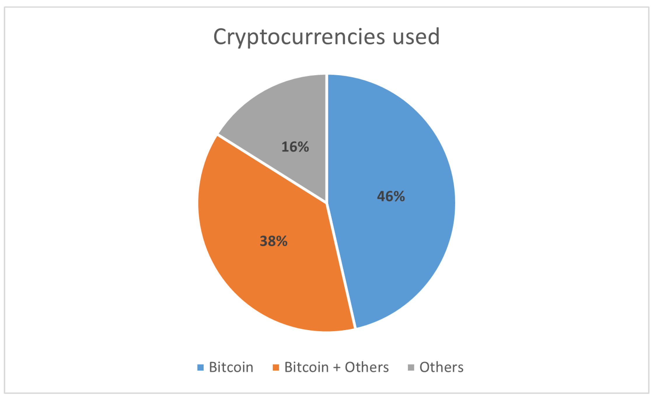
Figure 2.
Forecasting types present on the articles studied.
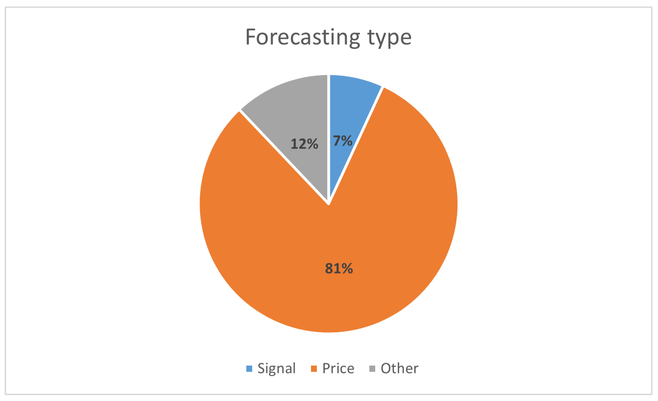
Figure 3.
Attributes used as predictors on the articles studied.
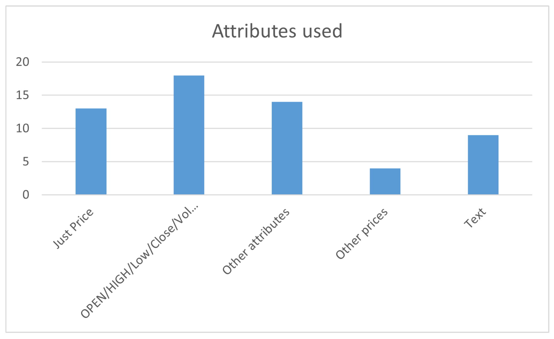
Figure 4.
Periods distribution on the articles studied.
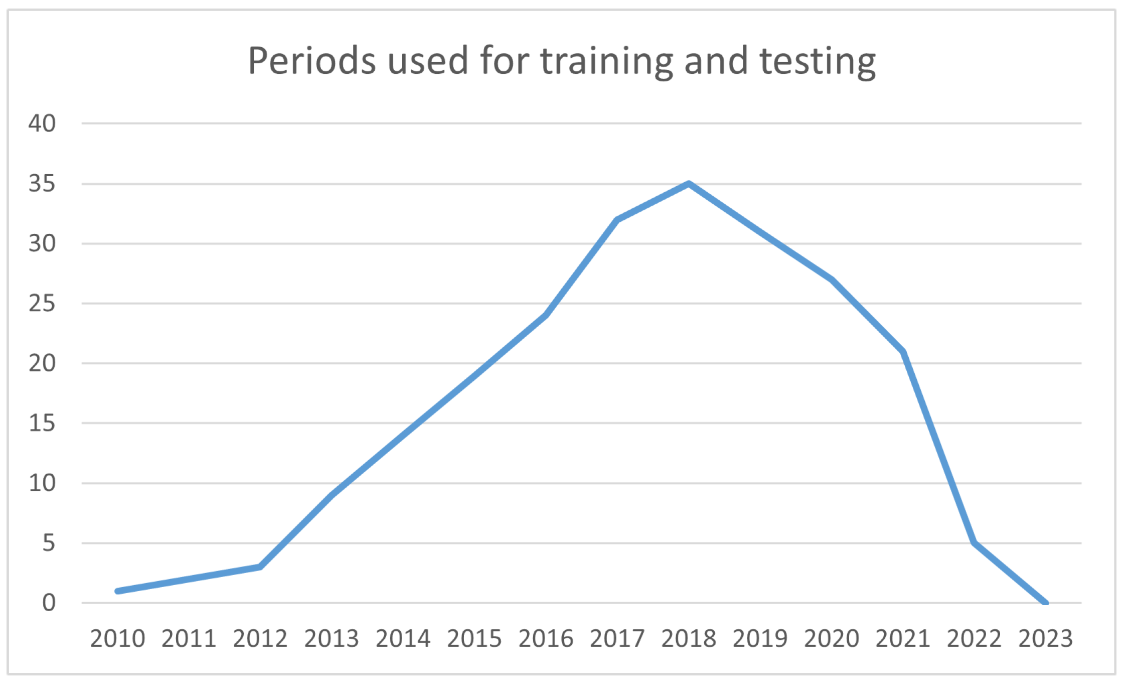
Figure 5.
Machine learning models distribution on the articles studied.
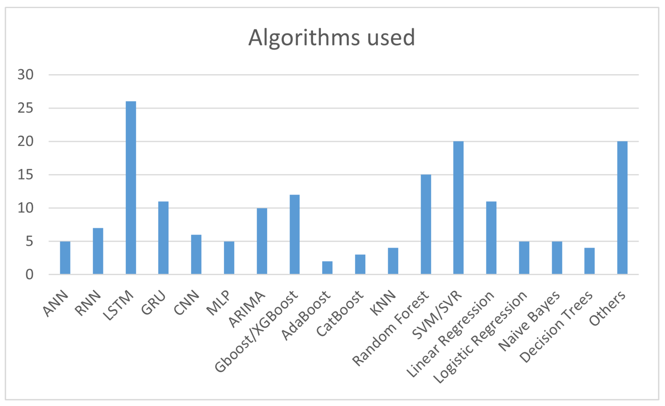
Figure 6.
Evaluation metrics used on the articles studied.
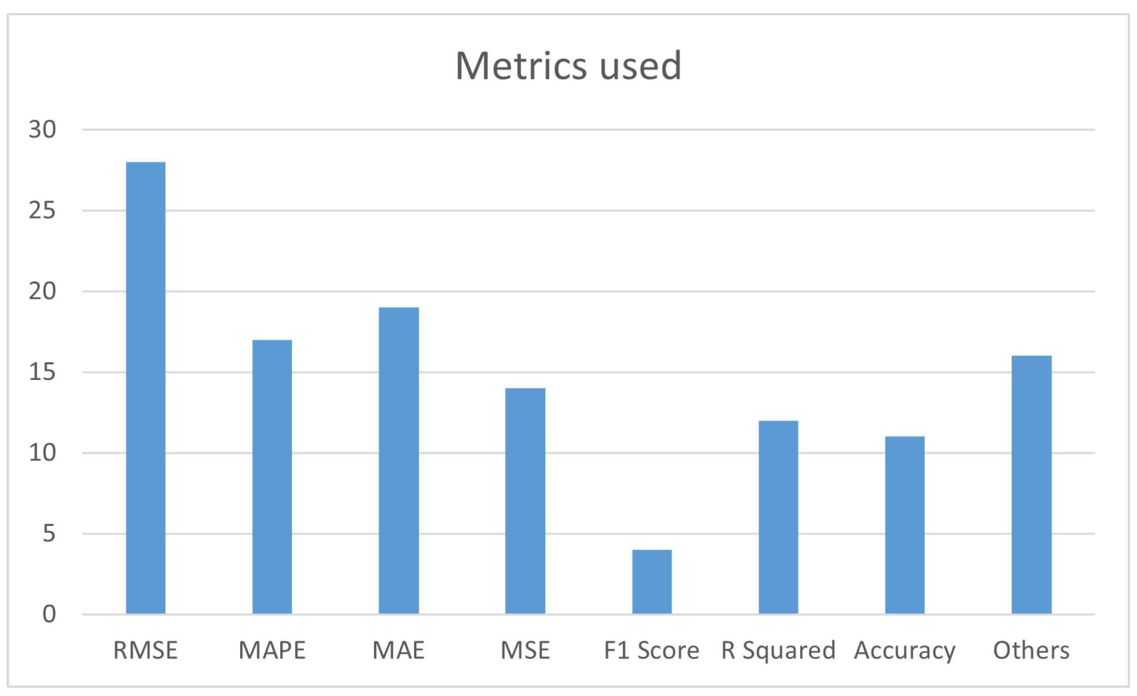
Figure 7.
Bitcoin, Ethereum, Binance Coin, Cardano, Solana, XRP, Polkadot, USD Coin, Dogecoin and Avalanche prices of the datasets used for model training and tests.
Figure 7.
Bitcoin, Ethereum, Binance Coin, Cardano, Solana, XRP, Polkadot, USD Coin, Dogecoin and Avalanche prices of the datasets used for model training and tests.
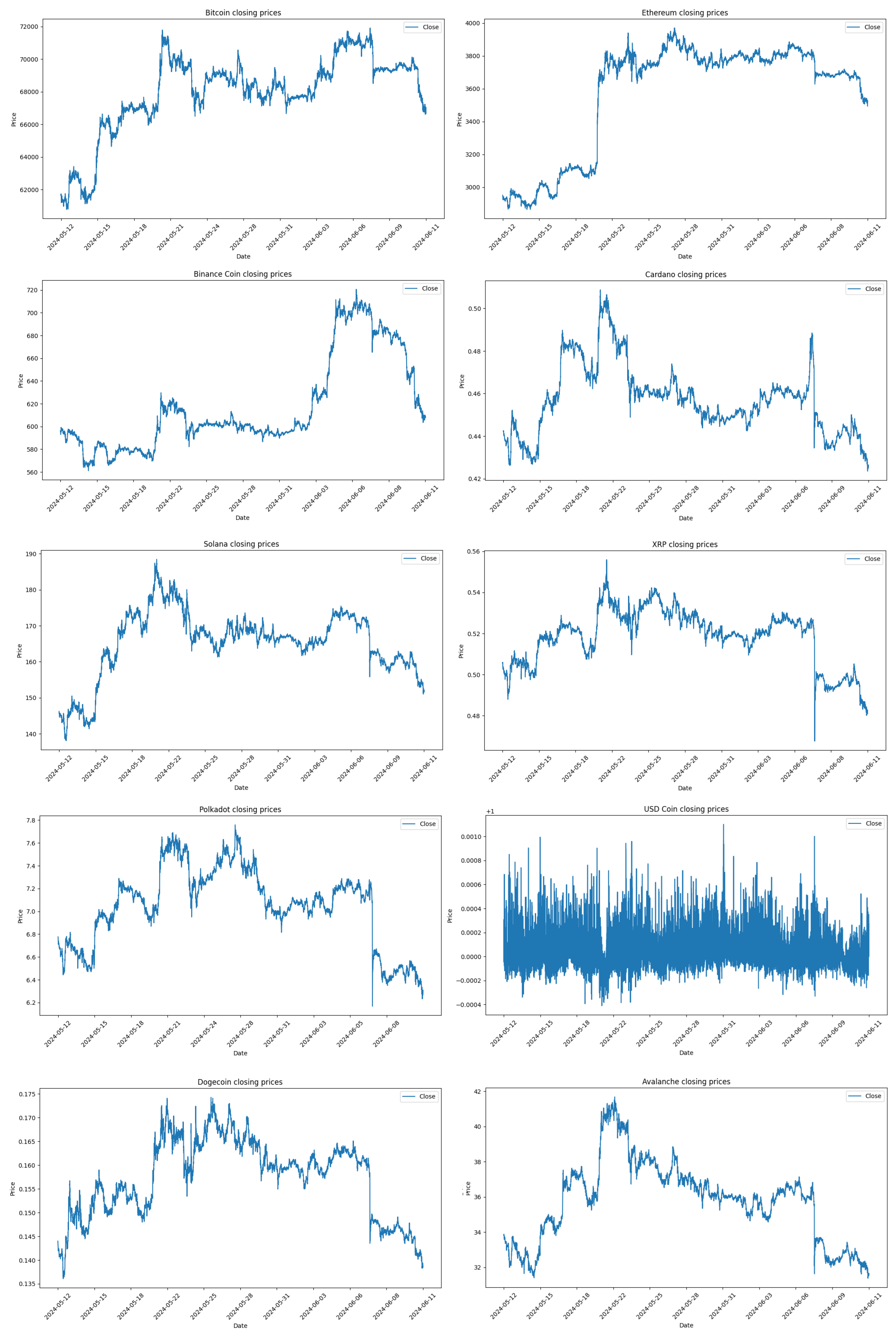
Figure 8.
Error metrics comparison for different forecast horizons.
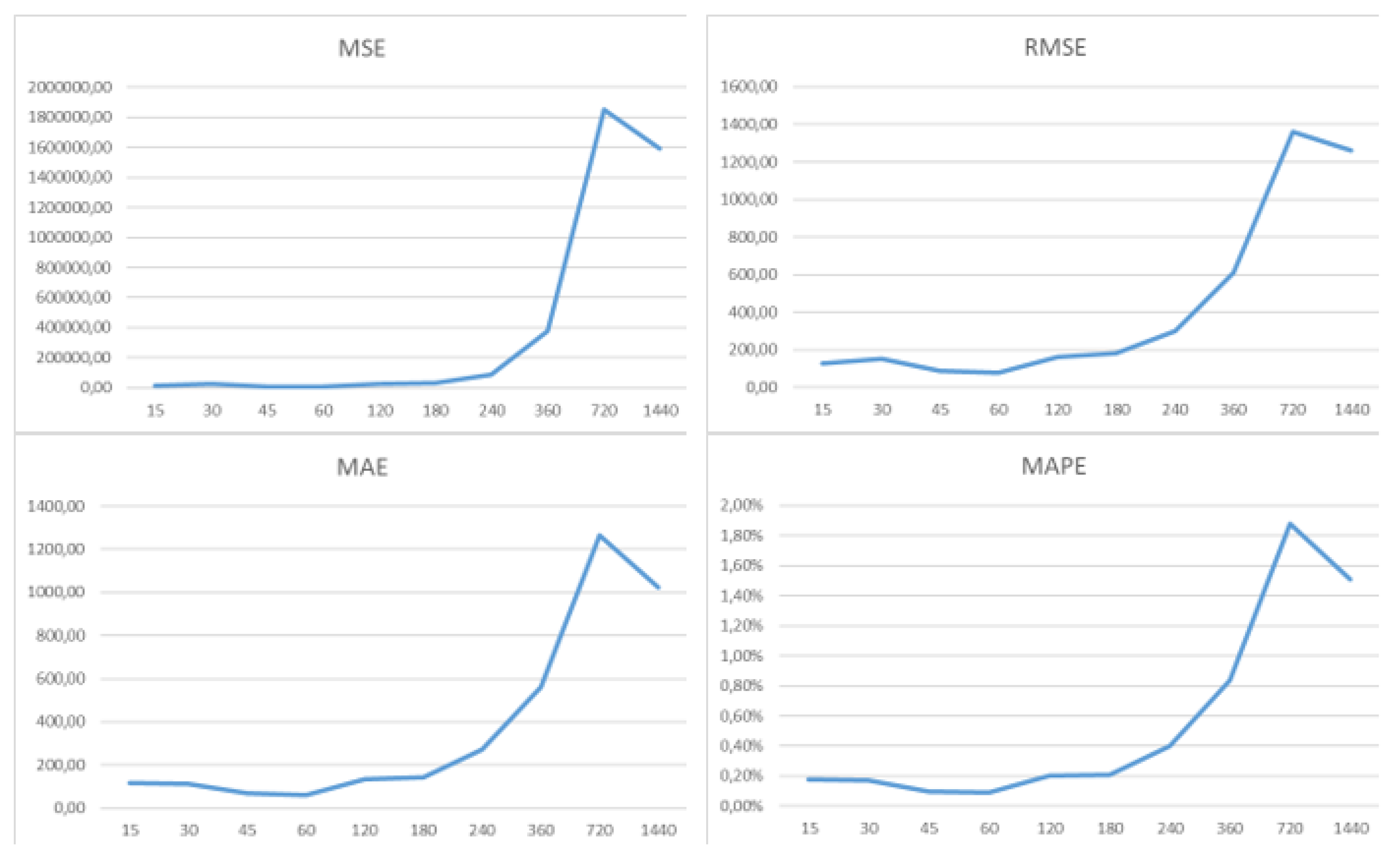
Figure 9.
MAPE and nRMSE comparison for all cryptocurrencies and different forecast horizons.
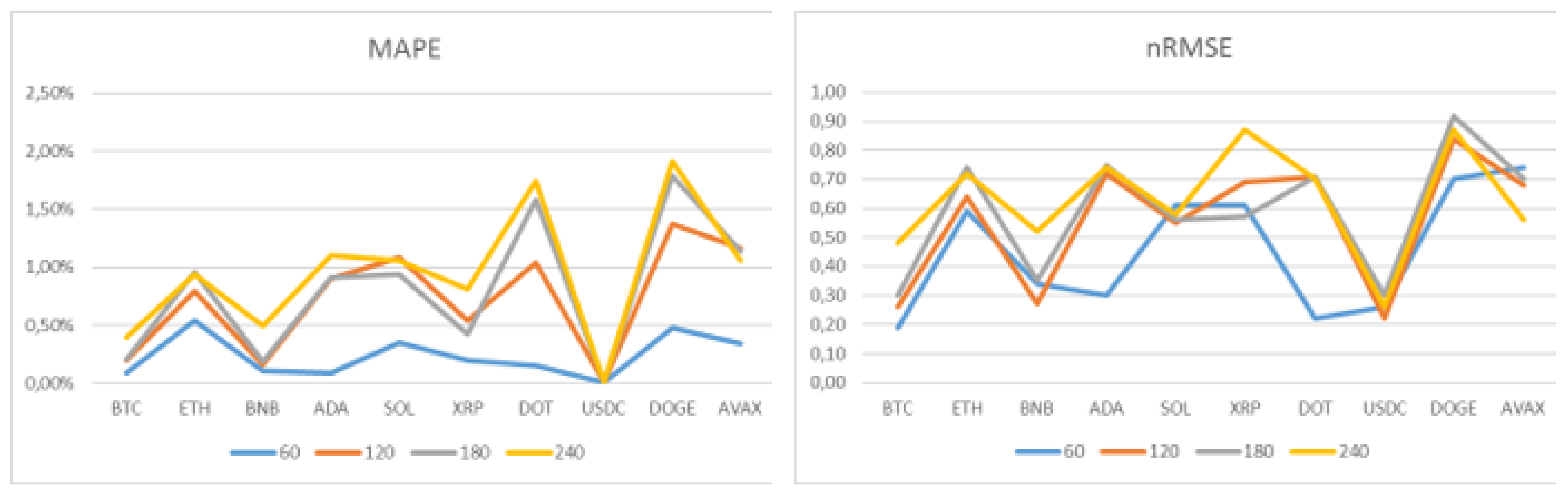
Figure 10.
Application structure.
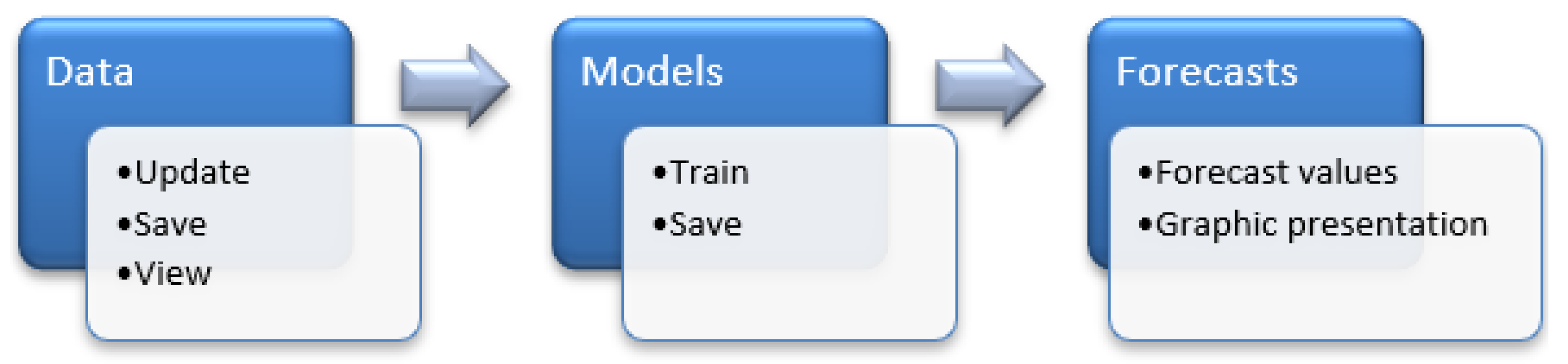
Figure 11.
App model train.
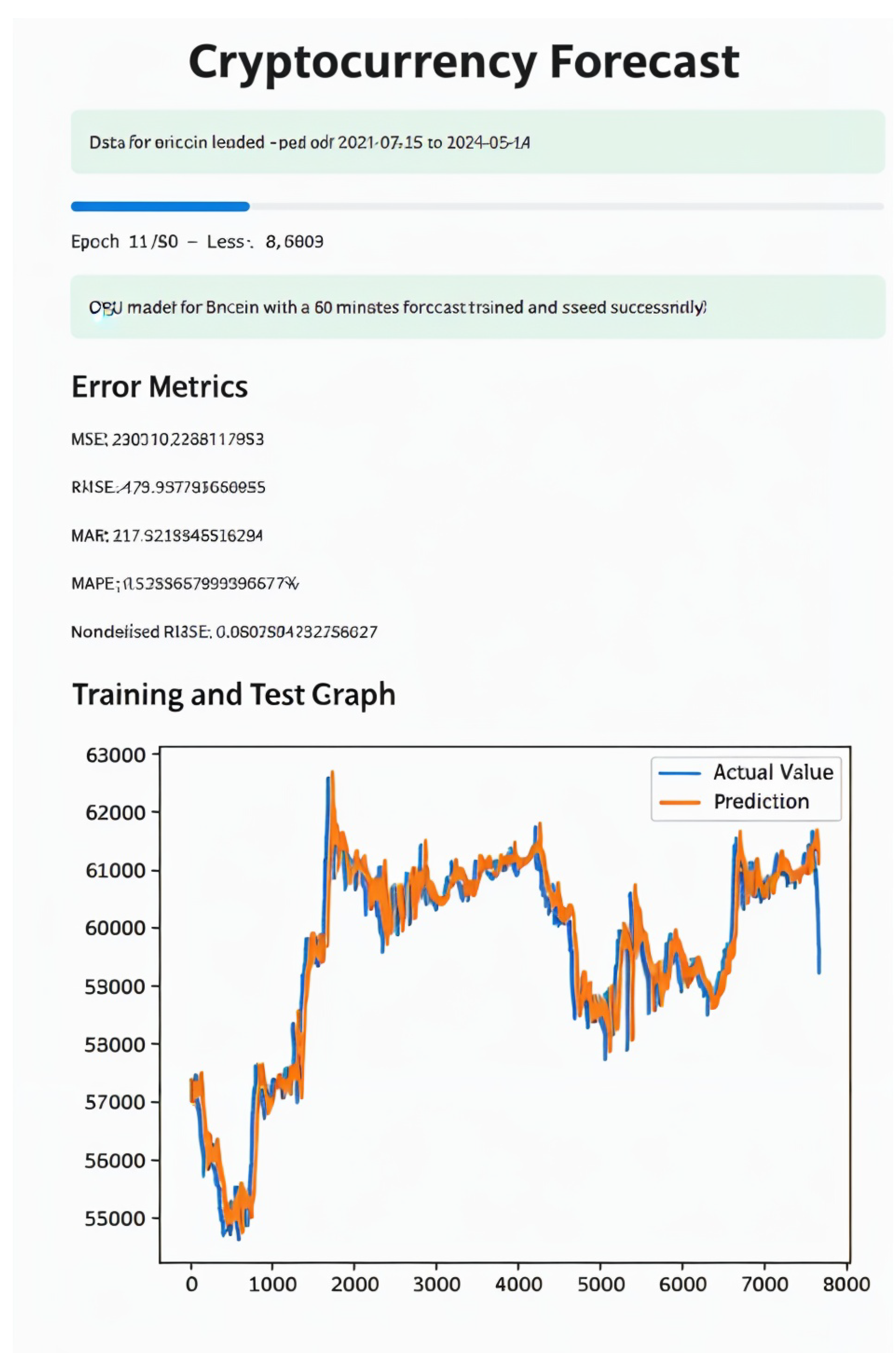

Table 1.
Statistics of evaluation metrics across all articles analyzed.
| RMSE | MAPE | MAE | MSE | F1 Score | Accuracy % | ||
| Max. | 7 527,300 | 26,653 | 6 631,800 | 2 159 166,250 | 0,920 | 0,998 | 99,690 |
| Min. | 0,007 | 0,000 | 0,002 | 0,000 | 0,611 | 0,639 | 55,940 |
| Average | 1 048,167 | 2,270 | 583,154 | 226 993,221 | 0,747 | 0,892 | 78,755 |
| Std. Dev. | 2 058,615 | 6,238 | 1 642,889 | 614 030,654 | 0,129 | 0,129 | 16,4512 |
Table 2.
Datasets - Closing prices.
| Count | Min. | Max. | Average | Std. Dev. | |
|---|---|---|---|---|---|
| Bitcoin | 33 781,00 | 60 787,36 | 71 907,85 | 67 948,15 | 2 425,81 |
| Ethereum | 38 216,00 | 2 864,56 | 3 969,70 | 3 570,00 | 340,87 |
| Binance | 37 923,00 | 561,14 | 720,60 | 617,54 | 41,25 |
| Cardano | 37 182,00 | 0,42 | 0,51 | 0,46 | 0,02 |
| Solana | 37 032,00 | 138,05 | 188,47 | 165,35 | 9,15 |
| XRP | 38 102,00 | 0,47 | 0,56 | 0,52 | 0,01 |
| Polkadot | 31 670,00 | 6,17 | 7,76 | 7,05 | 0,34 |
| USD Coin | 37 104,00 | 1,00 | 1,00 | 1,00 | 0,00 |
| Dogecoin | 38 052,00 | 0,14 | 0,17 | 0,16 | 0,01 |
| Avalanche | 37 076,00 | 31,37 | 41,68 | 35,76 | 2,28 |
Source: Yahoo Finance API. values from 12/05/2024 until 11/06/2024.
Table 3.
Datasets - Volume traded.
| Count | Min | Max | Average | Std. Dev. | |
|---|---|---|---|---|---|
| Bitcoin | 33 781,00 | 0,00 | 5 678 329 856,00 | 8 879 468,76 | 39 919 958,68 |
| Ethereum | 38 216,00 | 0,00 | 5 627 247 616,00 | 5 314 865,10 | 35 036 398,49 |
| Binance | 37 923,00 | 0,00 | 160 288 384,00 | 562 017,98 | 2 164 262,32 |
| Cardano | 37 182,00 | 0,00 | 36 492 032,00 | 124 569,45 | 544 606,32 |
| Solana | 37 032,00 | 0,00 | 495 197 696,00 | 915 416,00 | 3 743 308,07 |
| XRP | 38 102,00 | 0,00 | 210 166 016,00 | 367 591,09 | 2 000 541,95 |
| Polkadot | 31 670,00 | 0,00 | 18 362 512,00 | 76 259,87 | 305 245,21 |
| USD Coin | 37 104,00 | 0,00 | 994 848 256,00 | 1 986 002,90 | 12 395 098,23 |
| Dogecoin | 38 052,00 | 0,00 | 272 368 768,00 | 442 564,52 | 2 284 956,51 |
| Avalanche | 37 076,00 | 0,00 | 67 825 056,00 | 135 487,50 | 627 208,87 |
Source: Yahoo Finance API. Values from 12/05/2024 until 11/06/2024.
Table 4.
Models performance on 60-minute forecast of Bitcoin price.
| MSE | RMSE | MAE | MAPE | nRMSE | |
|---|---|---|---|---|---|
| Using all attributes | |||||
| LSTM | 8163,73 | 90,35 | 71,87 | 0,11% | 0,22 |
| GRU | 5954,89 | 77,17 | 60,20 | 0,09% | 0,19 |
| SARIMA | - | - | - | - | - |
| Lin. Reg. | 6979,26 | 83,54 | 64,36 | 0,10% | 0,20 |
| RF | 387460,75 | 622,46 | 572,41 | 85,55% | 1,50 |
| SVM | 10301,07 | 101,49 | 83,40 | 0,12% | 0,24 |
| XGBoost | 4206051,13 | 2050,87 | 1053,07 | 1,57% | 4,95 |
| LightGBM | 29859,99 | 172,80 | 137,39 | 0,21% | 0,42 |
| Using just the Close attribute | |||||
| LSTM | 7237,85 | 85,08 | 67,87 | 0,10% | 0,21 |
| GRU | 9307,22 | 96,47 | 75,98 | 0,11% | 0,23 |
| SARIMA | 19476,59 | 139,56 | 114,16 | 0,16% | 0,23 |
| Lin. Reg. | 6722,40 | 81,99 | 62,49 | 0,09% | 0,20 |
| RF | 38281,06 | 195,66 | 167,82 | 25,09% | 0,47 |
| SVM | 121987,11 | 349,27 | 338,49 | 0,51% | 0,84 |
| XGBoost | 37715,50 | 194,20 | 148,61 | 0,22% | 0,47 |
| LightGBM | 38132,43 | 195,28 | 165,60 | 0,25% | 0,47 |
Table 5.
GRU model performance for different forecasting horizons.
| Min. | 30 | 45 | 60 | 120 | 180 | 240 | 360 | 720 | 1440 |
|---|---|---|---|---|---|---|---|---|---|
| MSE | 23 634 | 7 786 | 5 955 | 25 713 | 33 575 | 89 106 | 375 233 | 1 854 184 | 1 589 417 |
| RMSE | 153,73 | 88,24 | 77,17 | 160,35 | 183,23 | 298,51 | 612,56 | 1 361,68 | 1 260,72 |
| MAE | 113,55 | 69,99 | 60,20 | 135,11 | 141,82 | 270,26 | 561,15 | 1 264,40 | 1 024,31 |
| MAPE | 0,17% | 0,10% | 0,09% | 0,20% | 0,21% | 0,40% | 0,84% | 1,88% | 1,51% |
| nRMSE | 0,37 | 0,21 | 0,19 | 0,26 | 0,30 | 0,48 | 0,62 | 0,73 | 0,36 |
Table 6.
MAPE and nRMSE values of the GRU model for all cryptocurrencies.
| MAPE | nRMSE | |||||||
| Cripto | 60 | 120 | 180 | 240 | 60 | 120 | 180 | 240 |
| BTC | 0,09% | 0,20% | 0,21% | 0,40% | 0,19 | 0,26 | 0,30 | 0,48 |
| ETH | 0,54% | 0,79% | 0,96% | 0,94% | 0,59 | 0,64 | 0,74 | 0,72 |
| BNB | 0,11% | 0,16% | 0,19% | 0,50% | 0,34 | 0,27 | 0,35 | 0,52 |
| ADA | 0,09% | 0,90% | 0,91% | 1,10% | 0,30 | 0,72 | 0,75 | 0,74 |
| SOL | 0,35% | 1,08% | 0,94% | 1,06% | 0,61 | 0,55 | 0,56 | 0,58 |
| XRP | 0,20% | 0,54% | 0,42% | 0,81% | 0,61 | 0,69 | 0,57 | 0,87 |
| DOT | 0,15% | 1,04% | 1,58% | 1,74% | 0,22 | 0,71 | 0,71 | 0,70 |
| USDC | 0,01% | 0,01% | 0,01% | 0,01% | 0,26 | 0,22 | 0,30 | 0,26 |
| DOGE | 0,48% | 1,37% | 1,79% | 1,91% | 0,70 | 0,84 | 0,92 | 0,87 |
| AVAX | 0,34% | 1,16% | 1,14% | 1,06% | 0,74 | 0,68 | 0,70 | 0,56 |
Table 7.
Performance comparison to related work.
| Ref. | Cripto | Forecast | RMSE | MAPE | MAE | MSE |
|---|---|---|---|---|---|---|
| [4] | Bitcoin | Price in 21 days | 251.61 | 0.31% | 164.49 | 63307.31 |
| [22] | Bitcoin | Daily price | 458.02 | - | 345512 | 209778.00 |
| [8] | Bitcoin | Daily price | 217,53 | 3,26% | 79,25 | - |
| [10] | Bitcoin | Daily price | 0,01 | 0,01% | 0,01 | - |
| [23] | Bitcoin | Daily price | 7 527,30 | 0,16% | 6 631,80 | - |
| [24] | Bitcoin | Daily price | - | 2,42% | 0,00 | 1,41 |
| [25] | Bitcoin | Daily price | 0,07 | 0,03% | - | - |
| [26] | Bitcoin | Daily price | 1 987,11 | 0,18% | - | - |
| [27] | Bitcoin | Daily price | 1 447,65 | 0,03% | - | - |
| [28] | Bitcoin | Daily price | 3 599,17 | - | - | 2 139,91 |
| [29] | Bitcoin | Daily price | - | 0,07% | - | 0,04 |
| [30] | Bitcoin | Preço diário | 1 469,41 | - | - | 2 159 166,25 |
| [31] | Bitcoin | Daily price | 372,84 | - | - | - |
| [32] | Bitcoin | 5 minute price | 1,44 | - | - | - |
| [33] | Bitcoin | 3 months price | 673,00 | - | - | - |
| [34] | Bitcoin | Daily price | 5 251,20 | - | - | - |
| [35] | Bitcoin | Daily price | 6 720,14 | - | - | - |
| [36] | Bitcoin | Daily price | 367,00 | - | - | - |
| [13] | Bitcoin | Daily price | - | 0,14% | - | - |
| [6] | Bitcoin | Daily price | - | 1,56% | - | - |
| [37] | Bitcoin | Preço diário | - | 1,69% | - | - |
| [38] | Bitcoin | 10 days price | - | - | 83,27 | - |
| [39] | Bitcoin | Preço diário | - | - | 0,02 | - |
| [40] | Bitcoin | Daily price | - | - | 0,02 | - |
| [41] | Bitcoin | 1 month price | - | - | - | 271,00 |
| [42] | Ethereum | Daily price | 253,68 | - | 115,91 | 64 355,56 |
| [43] | Litecoin | Daily price | 0,01 | - | 0,00 | 0,00 |
| [44] | Ethereum | Daily price | - | 0,75% | - | - |
| [45] | Cardano | Daily price | 0,60 | - | - | - |
Disclaimer/Publisher’s Note: The statements, opinions and data contained in all publications are solely those of the individual author(s) and contributor(s) and not of MDPI and/or the editor(s). MDPI and/or the editor(s) disclaim responsibility for any injury to people or property resulting from any ideas, methods, instructions or products referred to in the content. |
© 2025 by the authors. Licensee MDPI, Basel, Switzerland. This article is an open access article distributed under the terms and conditions of the Creative Commons Attribution (CC BY) license (http://creativecommons.org/licenses/by/4.0/).
Copyright: This open access article is published under a Creative Commons CC BY 4.0 license, which permit the free download, distribution, and reuse, provided that the author and preprint are cited in any reuse.


