Submitted:
21 July 2025
Posted:
22 July 2025
You are already at the latest version
Abstract
We investigate the key factors that shape the dynamic evolution of Day-Ahead spot prices of seven European interconnected electricity markets of the Core Capacity Calculation Region, Core CCR (Austria AT, Hungary HU, Slovenia SI, Romania RO), the Southeast CCR (Bulgaria BG, Greece GR) and the Greece-Italy CCR , GRITR (Italy), with emphasis on price surges and discrepancies observed in SEE CCR markets, during the period 2022-2024. The high differences in the prices of the two groups, has generated political reactions from the countries that ‘suffer’ from these price discrepancies, as shown by the intense reactions of the governments of the affected countries and other institutions, as the sending of letters of Prime Ministers European Commission President). By applying Machine Learning (ML) approaches, as Markov Blanket (MB) and Local, causal structures learning (LCSL), we are able of ‘revealing’ the entire path of volatility spillover of spot price as well as the Cross-Border Transfer Availabilities (CBTA) between the countries involved, from north to south, thus uncovering i.e. ‘lifting the blanket’, to discover the ‘true’ structure’ of the path of causalities, responsible for the price disparity. The above methods are supported by the ‘mainstream’ approach of computing the correlation of the spot price and CBTA’s volatility curves of all markets, to detect volatility spillover effects across markets. The main findings of this hybrid approach are: a) the volatility of Austrian market’s spot price and its CBTAs with DE, CZ, and SI, ‘uncovered’ to be a pivotal market, behaving as a ‘transmitter’ of spot price and cross-border activity volatility, over its entire connection path with SEE CCR markets, which finally ‘receive’ the volatility disturbances, causing their price surge, b) the combination of weather and geopolitical factors with the limited interconnectivity of SEE markets, seem to have exacerbated the impact of the Flow-based Market coupling method (FBMC) used in the Core CCRs, on the prices of SEE CCR’s countries that rely on the Net Transfer Capacity -NTC- mechanism, by inducing non-intuitive flows, thus challenging the reliability of European Target’s model (based on FBMC) in protecting SEE markets from ‘unexpected-unfair-irrational’ price surge.
Keywords:
Electricity wholesale electricity prices surge in SEE
; Local causality structure
; Markov blanket
; Bayesian tool
; wholesale Electricity prices
; spot price volatility spillover
1. Introduction
1.1. Price Disparity in Electricity Markets of Southeastern Europe (SEE) and Political Reactions
In this paper we present a ML approach in detecting the most critical and causal factors responsible for causing an unprecedented electricity spot prices surge, a phenomenon also called ‘European regional electricity crisis’, appeared mainly in Bulgaria (BG), Greece (GR), by analyzing the entire path of their interconnections with the ‘core’ countries of Austria, AT, Hungary (HU), Slovenia (SI) and Romania (RO), as well as the Greece- Italy interconnection. We note here that AT, HU, SI and RO are members of the Core CCR (Core Capacity Calculation Region) while BG and GR constitute the Southeast European SEE CCR (regions in which specific methodologies are used to compute cross-zonal capacities, see Section 3).
The ‘huge’ price disparity mainly in Bulgaria and Greece, and in Romania against the rest of the Core countries, challenges the capacity and success of the European electricity Target model, as we will see below. There are a variety of the factors that are behind this disparity, both ‘apparent and hidden’, as climatic, geopolitical and structural (generation mix, networks, interconnections), described in Section 3. The above countries that have been strongly affected took several initiatives to ease the pressure this disparity has imposed on their electricity Day-ahead prices. Among other reactions, they have prepared a proposal for the formation of a permanent intervention mechanism that would be triggered any time electricity prices turn extremely high in their markets, especially in cases where their region is disconnected from the rest of the core energy markets. A characteristic example of such reactions, is the letter of the Greek Prime Minister sent to European Commission President, to propose a set of measures [1]. Similar reactions were recently reported, as in Romania and in North Macedonia in which also an examination has initiated of the reasons for the huge price disparity. Another characteristic reaction is that of the Romanian Minister of Energy who sated that the country would ask the EU for compensation for this high price difference, but however listing several problems related to geopolitics (due to war in Ukraine), weather, power generation mix, and interconnections of his country with AT and other Core CCRs. Also at ministerial level, Greece, Bulgaria and Romania sat at the same table on 11th September 2024, with the three countries agreeing on the diagnosis of the problem. The three energy ministries drafted a text that was sent to the Commission, asking for flexibility from the relevant EU Directive for the implementation of a claw-back mechanism against high deviations in electricity prices. According to their draft text, this mechanism could be activated occasionally, for the imposition of a cap on the compensation of power plants and the recovery of excess revenues per technology, just as was done during the 2022 energy crisis. We point out here, however, that this mechanism (the request), in practice, cancels in practice the result of the Day-Ahead (DA) market price clearing methodology (the cornerstone of the European Target model), i.e. cancels the system's marginal price, which pays all units under this model, to contain large discrepancies. However, this objective seems to be very ambitious, as any modification on the core structure of the target model is a very crucial issue, and it needs the agreement of all involved markets’ ‘shareholders. As the Greek Prime minister said [1], ‘I do not expect that there will be immediate solutions to the problem, but at least let someone seriously deal with it, to highlight it, so that we can make sure that we do not have such distortions again in the future’.
1.2 Relating SEE CCR’s Price Discrepancies with Europe’s Target Model (TM). Is Its Algorithm an Incomprehensible Black Box?
After detecting the underlying crucial factors that have caused the discrepancies mentioned, it would be extremely interesting to examine whether these factors relate to the structural characteristics of the European Target model and more importantly, how this model has been performed in the case of the price surge mentioned. In fact, there are criticisms against the operational algorithm of the model, because at times, it seems that the algorithm has disconnected SEE countries from the rest of the European markets, turning the region into an energy island! The algorithm is based on the current mode of operation of electricity markets, which is different in Core CCRs and SEE CCRs, in respect of the way the available capacities in the zonal bidding-zones are calculated. More specifically, SEE CCR countries trade according to the net transfer capacity (NTC) mechanism, while the Core CCRs countries use the flow-based market coupling (FBMC) system (ACER 2024 report, [2]). A description of the above two mechanisms, the critical role they play in the formation of price surge in the SEE CCR, is given in Section 3 and Section 3.1. A notable ‘malfunction’ of the application of FBMC, as described in Section 3.1, is the production of counterintuitive power flows, that have drastically limited imports into high-demand regions like HU and RO, starting a price spike diffusion to ‘downstream’ BG and GR countries, a phenomenon challenging strongly the robustness of Europe’s ambitious TM, aiming at ensuring a fair and ‘homogeneous’ price landscape.
1.3. Characteristic Events in SEE CCR’s Markets, Core and Regional Structural Distortions
We give some critical events indicating the suffering of the SEE & RO electricity markets from extremely high prices. Due to exports to the North, in the evening (20:00) of 12 September 2024 in Greece, the maximum price was 485.60 euros per megawatt hour, while in Bulgaria 558.09 euros/MWh, in Romania 678.5 euros/MWh and in Hungary 667.75 euros/MWh (see Supplementary material C (table C3) for the maximum prices in the evening, hour 20:00, of 12th September 2024). For comparison, in the same period, in the Czech Republic the maximum price reached 242.87 euros/MWh and in Austria (a self-sufficient and net exporter market due to RES), at 256.15 euros/MWh. Thus, a price discrepancy (difference) of 161% against Hungary is observed which is not a conjunctural spread but rather seems to be a permanent phenomenon, not accepted in an environment of coupled markets. It is as if Greece and Bulgaria, two neighboring coupled market, have a price difference of more than 100 euros per megawatt hour, an unacceptable fact that challenges the way the Target Model operates in this region. Thus, intensive skepticism is diffused among the members of the SEE CCRs, based on such critical events as above, that the Core CCR countries, using a variety of ‘mechanisms’ in the Target Model’s FBMC approach can inhibit the normal energy outflows from their borders, reducing the capacity of cross-border transfer availability (CBTA). This occurred in the case of Hungary (HU), leaving the corridor between GR, BG and RO to meet Kiev's increased needs. This view is shared by the Greek and other governments in the region, as well as by other institutions as the president of the Greek Union of Industrial Consumers. It is broadly accepted that the ‘typical’ European electricity market is known to have some structural deficiencies-distortions that affect severely the competitiveness of EU’s member states (due to ‘systemically’ higher energy cost) [3], however due to the Ukraine crisis these distortions became more pronounced. Even at the borders of member states, for short distances, there exist price differences of 200, 300 or even 500 euros/MWh. The ‘mechanisms’ mentioned above refer to the advantages of the FBMC method in comparison to the Net Transfer Capacity (NTC) approach (in which cross-border transactions must cover at least 70% of interconnection capacity), followed by the SSE CCR countries (Section 3). The ‘mechanisms’ are considered responsible for the reduction or even zeroing, via a specific mathematical algorithm (characterized by the politicians as a black-box), of the capacity of cross-border interconnections. Besides the ‘core’ structural distortions emerging from the TM’s application on the region of the suffering markets, there are also other ones having regional effects. For example, in the interconnection of Greek and Italian electricity markets a ‘mechanism’ seems to exist, making almost systematically the Greek spot price to increase during the hours of peak demand. For example, in the evenings, constant electricity exports to Greece take place, making the cross-border transfer capacity between the two countries relatively ‘inadequate’ since the installed cable of 500 MW (at the time this report is written) becomes congested, and consequently disconnected from the system. Even more strange, the traditionally more expensive Italian wholesale market becomes cheaper than the Greek one. As an example, on 12thSeptember, at hour 20:00, the maximum price in the Italian energy exchange was 155.8 Euros/MWh, while the corresponding price in the Greek one reached at 485.60, a deviation of 212%!!
The rest of the paper is structured as follows: in Section 2 we provide a short literature review on the Markov Blanket-based causal feature selection accompanied by a description of Bayesian Analysis and Causality Structure Learning (CSL) approaches in electricity markets (extra information is also provided in Section 5). The crucial role of the power cross-border transfer availability between the markets analyzed, and especially its calculation method in Core CCR and SEE CCR counties, is discussed adequately in Section 3. The description of data sets used, their summary statistics and correlation analysis of the market’s variables, is given in Section 4. An extensive methodology of the MB and LCSL tools is provided in Section 5, which also contains practical issues in applying these methods in the field of electricity market analysis. The approach of rolling volatility of the crucial factors (extracted by the above tools) in causing the spot price surge as well as the volatility spillover effects in SEE markets, is described in Section 6. Section 7 provides the empirical results of both CSL and rolling volatility methods, with extensive comments, and finally in Section 8 we include a discussion, the conclusions and policy recommendations.
2. Literature Review on Markov Blanket-Based Causal Feature Selection
From our intensive literature review, we manage to locate a few specific research papers that apply Markov Blanket-based causal feature selection directly to energy market analysis. First, we have found several foundational works that discuss, in general, the use of Markov Blankets in causal discovery and feature selection, while in Section 2.2 we provide how MB has been adapted to energy market studies.
In the work of [4], the authors demonstrate how a generic feature-selection algorithm that returns strongly relevant variables can be transformed into a causal structure-learning algorithm. The authors prove this under the Faithfulness assumption for the data distribution. [5], provide a comprehensive review of feature selection and causal discovery research, summarizing theoretical results and presenting methods to enhance the scalability of discovery algorithms. A paper that discusses the use of Markov blankets in Bayesian networks for feature selection, addressing challenges when data distributions violate the faithful condition, and in which the authors propose the concept of representative sets to improve feature selection robustness, is the work by [6]. The study of [7] introduces a causal feature selection method based on an extended Markov blanket, aiming to reduce the number of features while retaining key ones. Experimental results demonstrate the method's effectiveness. The article of [8] explores the intersection of causal inference and feature selection, emphasizing the role of Markov blanket discovery algorithms in both fields. It discusses methods to enhance the efficiency of these algorithms. [9] summarize research on feature selection via the induction of Markov blankets over the past decade, providing insights into various algorithms and their applications. These papers mentioned above do not specifically address energy market analysis, however their methodologies have been adapted to study causal relationships and feature selection within that domain (see below). Applying Markov Blanket-based methods, in combination with LCSL methods to energy market data could help identify key factors influencing market dynamics, such as the dynamics of SEE price surges, by focusing on the most relevant variables and their causal interdependencies. Some areas on which MB has been successfully applied, are : a) healthcare: in predicting a disease, the Markov Blanket can identify the strongest causal factors (e.g., symptoms, genetic markers, lifestyle factors) while excluding irrelevant variables, b) in finance: for predicting stock prices, it can reveal key economic indicators, market trends, and company performance metrics that directly influence price movements, c) in marketing: in customer churn prediction, it can highlight the most influential factors (e.g., satisfaction scores, service usage patterns) while excluding noise.
Application of Bayesian Analysis and Causality Structure Learning Approaches in Electricity Markets
However, to the best of our knowledge, only a few papers dealing with the application of MB on analyzing energy markets were found in our literature review. [10] used a causality-based FS approach for data-driven dynamic security assessment of power systems. Their work describes how a probabilistic graphical model (of DAG type), tree augmented naïve bays structures, and an approximate MB, are used in building an online dynamic security assessment (DSA) framework. [11] have built an alternative approach to predictive modeling for energy demands, based on learning causality structure using demand date from an Argentinian electricity company. An improved, non-causal, feature selection algorithm of electricity price forecasting, using Support Vector Machine (SVM), is introduced by [12]. In their paper, the FS algorithm consists of threshold based mutual information (MI) (see Section 5.2), together with inequality correlations of symmetrical uncertainty and pairwise evaluation methods, to perform electricity price forecasting.
In [13] the authors have presented a Bayesian inference approach to unveil supply curves in electricity markets. In their study they introduced this approach, for revealing the aggregate supply curve in a day-ahead electricity market. Their proposed algorithm relies on Markov Chain Monte Carlo and Sequential Monte Carlo methods, and they argue that the major advantage of this approach is that it provides a complete model of the uncertainty of the aggregate supply curve, through an estimate of its posterior distribution. The authors have shown, in a small case study, that it is possible to reveal accurately the aggregate supply curve with no prior information on rival participants, information that can be used by a price-maker producer to devise an optimal bidding strategy.
In [14], the authors have applied Bayesian Belief Networks in the modelling of wholesale electricity price formation, specifically in power systems with a high penetration of non-firm renewable generation. Their work links the mathematical Bayesian representation to established statistical and computational approaches using a functional supply-side wholesale electricity market pricing model and introduces a novel validation method employing volatility analysis to assess the case study’s performance. Their work is valuable in examining the transition of electricity generation from firm to non-firm renewable generation, a factor that creates changes in wholesale electricity price dynamics, therefore challenging existing modeling approaches due to the stochastic nature of wind and solar as the primary energy source. They showed that constructing robust pricing models essential for optimizing financial performance in today’s electricity markets, can be greatly facilitated by using their Bayesian Belief Networks approach.
The aim of the paper in [15], is the study of Bayesian forecasting of electricity prices traded on the German continuous intraday market which fully incorporates parameter uncertainty. Their target variable was the IDFull price index, and the model’s forecasts were provided in terms of posterior predictive distributions. They validated the results, using the exceedingly volatile electricity prices of 2022. The IDFull index is the weighted average price of all continuous trades executed during the full trading session of any EPEX SPOT continuous contract. This index includes the entire market liquidity and thus represents the obvious continuous market price references for each contract.
In [16] researchers have used Bayesian networks for analysis and prediction, to understand the causal relationships between variables such as consumption, greenhouse emissions, investment in renewables and investment in fossil fuels, towards making a reliable energy policy focusing mainly on renewable energy sector, and not only by observing energy scenarios in various economic or social conditions. In their paper have presented expert models using the capabilities of Bayesian networks in the renewable energy sector, considering renewables in Germany and Italy, using the tool BayesiaLab (a powerful desktop application-Windows/Mac/Unix- for knowledge management, data mining, analytics, predictive modeling and simulation, all based on the paradigm of Bayesian networks), with supervised learning, on a data set consisted of the consumption rate of geothermal and hydro energy sectors. They have found that, as oil prices grow, greenhouse emissions will decrease, and that the precision of the expert model is no less than 90%.
In the paper [17], the authors have provided for the first time a complete literature review in the application of Bayesian networks in renewable energy systems, for which the implementation of conventional methods does not solve the problems associated with the complexities of these systems. According to the authors, recently, Artificial Intelligence techniques such as Artificial Neural Networks, Fuzzy Logic and Genetic Algorithms, have been widely used to deal with these problems in the field of Renewable Energy. However, the degree of uncertainty that is involved in these methods needs Bayesian Networks since this is one of the most effective theories to face them. In their work, they present the state of art of the applications of Bayesian Networks in Renewable Energy, such as, solar thermal, photovoltaic, wind, geothermal, hydroelectric energies and biomass, including related topics such as energy storage, smart grids and energy assessment. They have found that the main applications were in forecasting, fault diagnosis, maintenance, operation, planning, sizing and risk management, and they argue that Bayesian Networks constitute a powerful and versatile tool for the field of Renewable Energy.
With the rapid development of the economy, fully leveraging the priority role of electricity is of great significance for accelerating the modernization of electricity, continuously meeting the growing demand for electricity and social production and consumption and promoting socio-economic development. Among them, the role of electricity marketing is becoming increasingly prominent. How to fully mine and utilize the large amount of power marketing data accumulated by electric power enterprises over the years, to provide reliable support for the analysis and research of power marketing decisions. Bayesian network is a graphical pattern used to represent the continuous probability distribution of a set of variables, which provides causal information to discover potential relationships between data, and because of these characteristics, it is widely used in data mining.
In the work of [18], researchers apply Bayesian network to the analysis and research of power marketing decisions and establishes a Bayesian network suitable for power marketing decision-making for customer value evaluation, providing reliable support for marketing decision-making. They emphasized the ability of Bayesian network of making good decision models, based on their feature of making graphical patterns used to represent the continuous probability distribution of a set of variables, which provides causal information to discover potential relationships between data.
3. Power Cross-Border Transfer Availability in Core and Southeast Europe Capacity Calculation Regions (CCRs) and Its Impact on the SEE Markets Spot in Prices
Between 2022 and 2024, cross-border electricity transfer availability in Central Eastern and Southeastern Europe (CEE and SEE) significantly influenced wholesale electricity prices, particularly in the SEE region. Cross zonal trading opportunities are critical in curbing Day-Ahead or spot price volatilities. Due to insufficient cross-border transfer availability in year 2023, an explosion in negative DA prices (see Figure 5 and Table 4, Table 5 and Table 6 in this paper) occurred, because a low electricity demand coincided with an increased renewable supply in each bidding zone1. According to Figure 1 of ACER’s 2024 report [2] , Greece (GR) exhibited zero occurrences of spot negative prices, BG 11, RO 32, HU 74, AT 111, SI 96 and IT-South zero negative prices, emphasizing the need for the markets with negative prices, for local flexibility and the criticality of the cross-zonal transmission capacity (measured by CBTAs in our data set). Another crucial parameter as well as a proxy for the level of implementation of a ‘really successful’ integration of the EU power systems, related to the cross-border capacity, is the price convergence of bidding zones within Capacity Calculation Regions (CCR), in the wholesale market. During 2023, GR-IT CCR the price convergence (% of hours) was moderate2 (16%) and full (28%), while in 2022 the values were 8% and 28% respectively [2]. According to the same report, the most crucial factors explaining the price convergence are the differences in the generation mixes, the way the implicit market coupling in DA markets is implemented and finally, and most important for the targets of our study, the level of transmission capacity available for cross-zonal trade (our CBTA variable). Thus, detecting the most crucial factors shaping the price surge and discrepancy between Core markets (AT, SI, HU and RO) and the SEE markets of BG and GR, is strongly linked to the above crucial factors in explaining price convergence, between the Core Capacity Calculation Region (Core CCR) of the core markets and the SEE CCR markets, two CC regions using different capacity calculation methods3, the Flow-Based (FB) in Core CCR and Coordinated Net Transfer Capacity (CNTC), in the SEE CCR (the CBTAs in our data set are calculated by the CNTC methods, used by the TSO of the specific region). Table 1 (our elaboration based on data from [2]) informs about the implementation status of the Regional Capacity Calculation methodologies, for the markets analyzed in the present work. In 2023, the level of cross-zonal capacity offered, on average, in the biding zone borders of Core, GRIT and SEE CCRs, for the spot market is: 2100 MW Core, 2090 GRIT and 1200 MW SEE.
We now give some information, based also on [2], about the yearly evolution of transmission capacities available for cross zonal trade in the Day-Ahead market, that we consider to be very related to this analysis. More specifically, the level of interconnectivity of Member States calculated as the yearly average offered import capacity of every Member State as a percentage of peak electricity demand, and the yearly average offered export capacity of every Member State as a percentage of peak generation. Table 2 provides such information, from which we observe that the markets of Core CCRs show significantly larger levels of connectivity than the SEE CCRs and the GRIT CCR. This important information shows that the Core CCR markets included in flow-based market coupling in 2024 (also in 2022 and 2023) exhibit a considerable increase in their levels of interconnectivity, as measured by the above two measures. In general, as we have already mentioned, FB market coupling generally offers more exchange possibilities than NTC calculation, because it incorporates the modelling of the underlying electricity network in the allocation of cross-zonal capacities. The maximum import and export capacities in FB regions on a given bidding zone border are dependent on other exchanges in the region, which is not the case for NTC values, which are simultaneously feasible on all bidding zone borders. FB optimization-oriented approach leads to available capacities on specific network elements being allocated where they generate most socio-economic welfare.

Table 1.
Implementation status of the Regional Capacity Calculation methodologies, for the markets analyzed in this report (Based on data in [2]).
Table 1.
Implementation status of the Regional Capacity Calculation methodologies, for the markets analyzed in this report (Based on data in [2]).
|
Capacity Calculation Region (CCR) |
Calculation approach |
Day Ahead | |
| Regulation* | Implementation Status | ||
| Core: AT, HU, SI, RO | FB Coupling | Capacity Allocation and Congestion Management (CACM) |
Mostly |
| GRIT: GR, IT | Coordinated net Transfer capacity CNTC |
Capacity Allocation and Congestion Management (CACM) |
Mostly |
| SEE: BG, GR | Coordinated net Transfer capacity CNTC |
Capacity Allocation and Congestion Management (CACM) |
Mostly |
| *Note: Article 34 of regulation (EU), 2015/1222 | |||
To ensure that cross-zone capacity offered to the market is always efficiently allocated, all EU bidding zones borders, are now included in the Single DA-Coupling (SDAC) and the Single Intraday Coupling (SIDC), a very significant progress. In 2029, the EU Electricity Regulation [54], has ‘forced’ TSOs to offer the market a minimum level of cross-zonal capacity (CZC), considering however each TSO’s operational security limits. In 2020 a 70% minimum was imposed for implementing the requirement, without risking system security, allowing also the TSOs to opt for a transitional period. In this research paper, we assume that the way each TSO in the above CCRs (Core and SEE) have reacted to this 70% minimum of cross-zonal capacity has affected the dynamic evolution of the CBTAs of each market analyzed and consequently the spot price discrepancy between Core and SEE CCRs.
Table 2.
Level of interconnectivity of Member States in the day-ahead market measured as the average yearly import capacity as a percentage of peak demand and peak generation, in 2024.
Table 2.
Level of interconnectivity of Member States in the day-ahead market measured as the average yearly import capacity as a percentage of peak demand and peak generation, in 2024.
| Capacity Calculation. Region (CCR) |
As % of peak demand (2024) |
As % of peak Generation (2024) |
|---|---|---|
| Core: AT, HU, SI, RO | 75, 102, 224, 47 | 53, 129, 273, 34 |
| GRIT: GR, IT | 11, 13 | 11, 4 |
| SEE: BG, GR | 32, 11 | 29, 11 |
Limited Cross-Border Capacity and Market Fragmentation
The minimum 70% requirement translates in practice into the margin made available for cross-zonal trade MACZT), which is so a proxy for the level of integration of EU national day-ahead electricity markets. MACZT corresponds to the portion of capacity of a given CNEC that is made available for cross-zonal trade by the TSOs. The current level of optimization of the cross-zonal electricity transmission infrastructure across European spot markets, as well as the degree of the 70% implementation requirement is assessed by a MACZT monitoring report. However, despite EU regulations mandating that at least 70% of cross-border transmission capacity be available for electricity trading by the end of 2025, many regions in both Core CCR and SEE CCR, fell short. For example, based on the ACER’s report 2024 [2], during 2023, from the Core regions, only SI has achieved a value 97% of MACZT , (i.e. the % of hours when the minimum hourly MACZT was above 70% ), while the values of this index for other markets, in the same period, were: for AT 20% MACZT<50%, for HU only 6% for MACZT > 70 and 61% in the range 50% MACZT<70%, and RO 95% in the range 20% MACZT<50%.
Regarding the SEE CCR, encompassing the bidding zone borders Romania-Bulgaria and Bulgaria-Greece, in which the CNTC method is applied, the percentage of hours when the relative MACZT was above the minimum 70% requirement or within predefined ranges, in 2023, are as follows (ACER, 2024) : a) Bulgaria : for BG>GR and GR>BG no limiting element in the Member State, b) Greece: for BG>GR, 44% in range MACZT , 43% in range 20% MACZT<50%, while for GR>BG, 75% in range MACZT and 14% in range 50% MACZT<70% , and finally c) Romania: for BG>RO only 9% in MACZT , 53% in 20% MACZT<50% and 21% in MACZT<20%, while for RO>BG only 18% in MACZT 20% MACZT<50%, 21 % in range 50% MACZT<70% and finally 14% in MACZT<20%. The above-mentioned report also presents the percentage of hours when the limiting CNEC was, from the perspective of every Member State, located in the neighboring Member State, and therefore the TSO had no limiting CNEC to report. The report shows that this was particularly evident in the case of Bulgaria, for which the limiting CNEC on the Bulgaria–Greece and Bulgaria–Romania borders is often located in Greece and Romania, respectively. It is worth mentioning that in 2020, the SEE CCR achieved this 70% minimum target only 8% of the time, indicating substantial underutilization of interconnectors.
While the above information shows the extent to which Member States in the SEE region offered a minimum of 70% MACZT on its limiting CNECs in 2023, it does not include any information regarding the reasons for deviating below 70%. During the capacity validation period, reductions of capacity may be sent by either TSO on each bidding zone. During 2023 most limitations in the SEE CCR have been requested by the Bulgarian TSO, affecting so the MACZT results of the Greek and Romanian TSOs. A very important finding from comparing the Core and SEE CCRs adaptation in the 70% requirement is that the capacity calculation methodology implemented in the latter region does not have any specific provision in order the calculated capacities to adjust accordingly to comply with the minimum cross-zonal capacity requirements, Of course, such a provision must consider the remedial action potential in each market of the region. Due to this, a relatively poorer performance is observed in the SEE CCR in 2023. According to ACER’s 2024 report, Greece has requested a derogation in applying the requirement. Specifically, the derogation requested by the Greek TSO does not include a commitment on the levels of MACZT offered but sets a minimum value of 15% of the MCCC, a commitment that in Greece has been largely met in 2023. The same cannot be said about Romania’s action plan linear trajectory value of 43% of the MACZT in 2023.
For the Greece-Italy CCR, the Percentage of hours when the minimum hourly MACZT was above 70% or within predefined ranges in the GRIT CCR for each Member State and oriented bidding zone border – 2023 (% of hours) are as follows: a) for GR: 78% in range MACZT , for both GR>IT-South and IT-South>GR, while for b)Italy, 76% in range MACZT , for IT-South>GR. We note here that the GRIT CCR contains the internal Italian bidding zone borders and the DC bidding zone border with Greece, thus the impact of exchanges with third countries is considered limited. Additionally, thanks to the grid structural specifications, the impact of exchanges across other borders within the region is considered negligible (ACER, 2024).
From the above we conclude that SEE CCR’s limited capacity may have hindered electricity imports during periods of high demand, contributing to price spikes. Furthermore, the SEE region's reliance on the Net Transfer Capacity (NTC) mechanism, as opposed to the Flow-Based Market Coupling (FBMC) used in Central and Western Europe, exacerbated market fragmentation. FBMC's complex algorithms (a critical feature of the Target model) sometimes resulted in counterintuitive power flows, limiting imports into high-demand regions like Hungary and Romania, and leading to significant price disparities.
Figure 1 and Figure 2 show the time series of CBTAs of Austria’s CBTAs with Hungary, Slovenia, Italy and Germany-Luxembourg, and between Romania and Bulgaria (RO-BG, BG-RO), Greece and Bulgaria (GR-BG, BG-GR), respectively. In Figure 3 we show the DA prices of the markets involved in the previous cross-border transactions, for a visual inspection of how these prices have been affected by CBTAs. In July 2024 (see Figure 1), reduced imports to Hungary occurred, a notable event highlighting FBMC's shortcomings. More specifically, after July 8, FBMC allocations from Western Europe to Hungary decreased by approximately 1,200–1,300 MW during peak evening hours (19:00–24:00). This reduction was not due to maintenance or physical grid constraints but stemmed from FBMC's algorithmic decisions. Consequently, Hungary's HUPX market (Hungarian Power exchange, https://hupx.hu) experienced price surges up to €940/MWh, while neighboring Austria's prices remained around €61/MWh, illustrating a stark disparity across an internal EU border (see Figure 3). Almost concurrently, counterintuitive flows to Romania happened (see Figure 2). Romania faced reduced imports from Bulgaria due to maintenance on the BG>RO interconnector, decreasing capacity from 1,700 MW to 1,200 MW. To compensate, FBMC facilitated increased imports from Hungary. However, this led to situations where Romania's OPCOM market (the Romanian Electricity and Gas Market Operator) had prices up to €250/MWh lower than Hungary's HUPX, despite importing electricity from Hungary. Such non-intuitive flows strained Hungary's market further and underscored FBMC's limitations in addressing regional demand effectively.
Figure 1.
The cross-border transfer availabilities (CBTAs) between HU and AT, SI and AT, IT and AT, and DE and AT. (All countries are in the Core CCR). Total flows, i.e. (+) from HU to AT and (-) from AT to HU.
Figure 1.
The cross-border transfer availabilities (CBTAs) between HU and AT, SI and AT, IT and AT, and DE and AT. (All countries are in the Core CCR). Total flows, i.e. (+) from HU to AT and (-) from AT to HU.
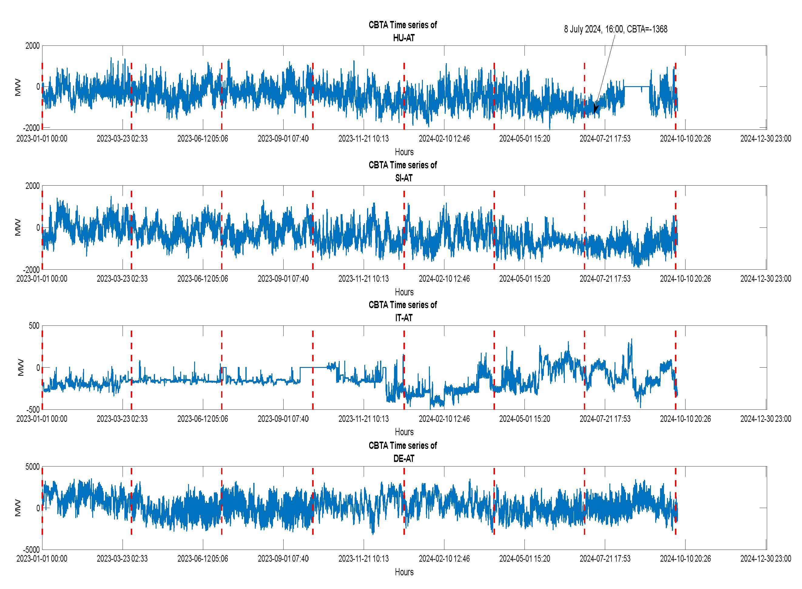
Figure 2.
The cross-border transfer availability (CBTA) between RO and BG, and between GR and BG countries. (RO is in the Core CCR, and GR and BG in the SEE CCR).
Figure 2.
The cross-border transfer availability (CBTA) between RO and BG, and between GR and BG countries. (RO is in the Core CCR, and GR and BG in the SEE CCR).
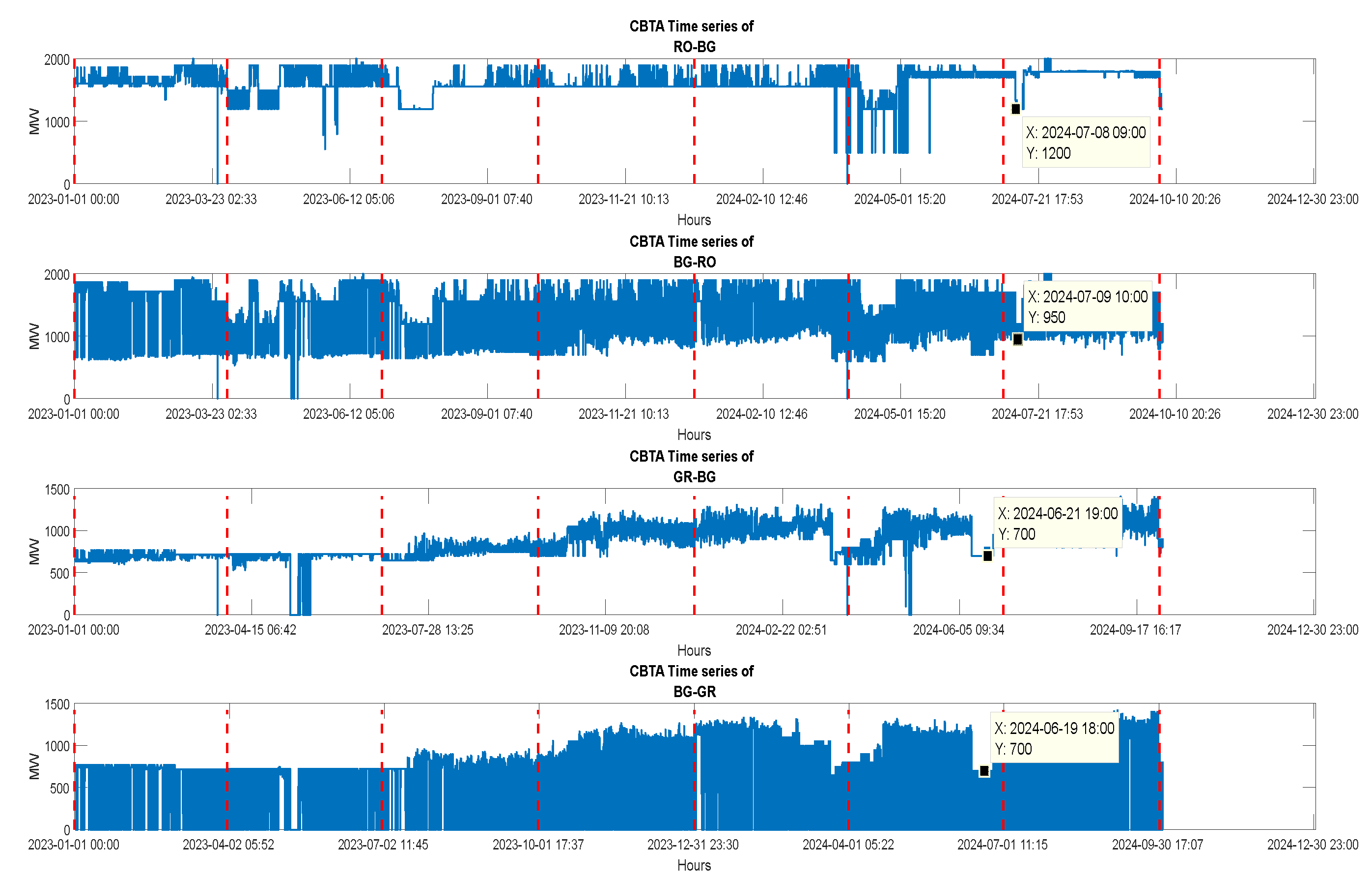
Figure 3.
DA-prices of AT, HU (Core CCR), and BG, GR (SEE CCR) markets.
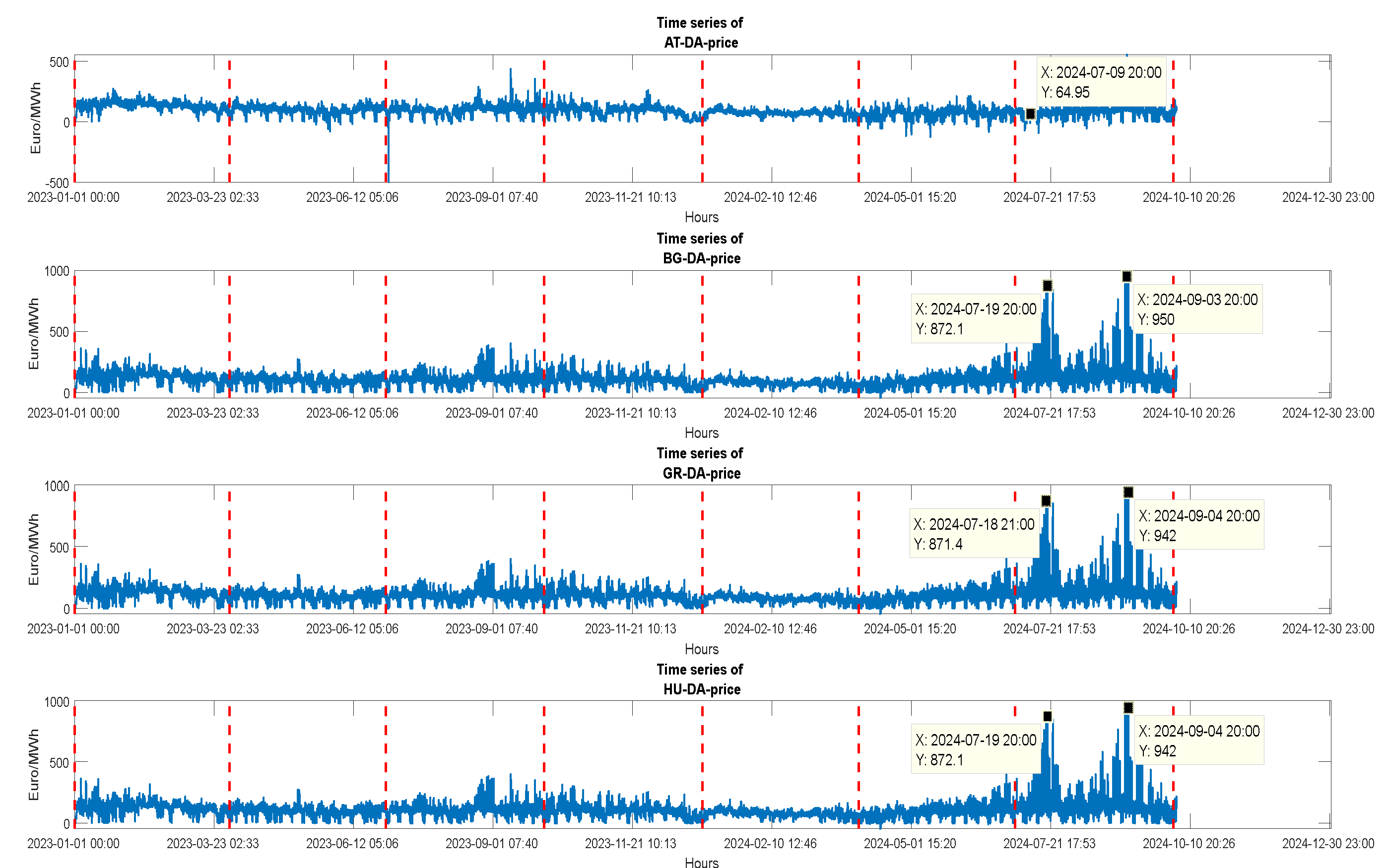
Several external factors have also enhanced the impact of limited cross-border capacity. More specifically, climate events such as record-high temperatures and droughts in SEE regions have reduced hydropower output and increased electricity demand for cooling, stressing the already constrained grid. Additionally, geopolitical tensions as the Russia-Ukraine conflict, disrupted energy supplies, with Ukraine, as we already mentioned, transitioning from an electricity exporter to an importer, increasing demand on neighboring countries' grids. Finally, infrastructure limitations, as delays in returning key power plants, like Bulgaria's Kozloduy nuclear plant, to full operation, reduced available generation capacity (the plant disrupted one of its two reactors, for a period until November 30, 2024, with the consequence the regional system to have 1 GW less). These factors have contributed to unprecedented wholesale electricity price spikes in the SEE region. Based on Figure 3, in August 2024, Greece's electricity prices more than doubled from €60 to €130 per megawatt-hour (MWh). Hungary (HU) experienced prices as high as €940/MWh during peak hours, while neighboring Austria (AT) saw prices around €61/MWh, highlighting severe regional disparities. Romania (RO) and Bulgaria (BG) also faced significant price increases, with day-ahead market prices reaching €700/MWh and €500/MWh, respectively. The findings above have stressed the importance of the interactions of volatilities of spot prices and CBTAs, that are enhanced further by the combined influences of external factors, geopolitical tensions and infrastructure limitations (as the limited interconnectivity of SEE countries, emerging from their reliance on the Net Transfer Capacity (NTC) mechanism, contrasting with FBMC's application in Central Europe, a critical discrepancy that hinders seamless integration and efficient electricity distribution). All these findings challenge the status of the current policy, an issue discussed in Section 8.
4. Data Sets, Preprocessing, Summary (Descriptive) Statistics, Correlation Analysis and Cross-Border Transfer Availability
We use data downloaded from ENTSO-E Transparency platform (transparency@entsoe.eu), for our set of seven electricity markets, including Austria (AT), Bulgaria (BG), Romania (RO), Slovenia (SI), Greece (GR), Hungary (HU), and Italy (South bidding zone) (ITsouth), from January 2022 to October 4, 2024. We analyze hourly wholesale price data expressed in in Euro/Mwh. The countries under analysis are shown in Figure 4, which also depicts the borders where the calculation of the Capacity from the interfaces changes from Net Transfer Capacity (NTC) to Flow Based (FB) [2]. The dataset covers the period from 1.1.2022 to 4.10.2024, their missing values have been filled appropriately, with frequency converted from originally 15 minutes to hourly data. Thus, the size of dataset is 24194. Figure 5 shows the time series of hourly spot prices of all markets for the period of 1st January 2022 to 4 October 2024, and Figure 6 the time series of Greek DA hourly spot prices. Two distinct periods of high spot prices and volatility, in all markets of our analysis, are observed in Figure 5. The first is from early spring (March) of 2022 to December 2022, with a pronounced upward and downward price oscillations, and a peak price occurring on 30th of July (1041 Euro/MWh). The second period covers the summer of 2024, ending approximately at the end of August 2024. We describe shortly at this point the main drivers that seem to be the prevailing factors in shaping the price dynamics shown in Figure 5. For the 2022 price surge the main drivers are : a) gas crisis from Russia’s Invasion of Ukraine, since Russian pipeline gas flows into Europe plummeted, TTF gas prices spiked over €300/MWh in late August 2022, and finally power prices in gas-dependent regions soared as gas-fired generation costs increased dramatically, b) high CO₂ Prices, EU ETS prices sustained levels above €70–€90/tonne, resulting to elevated variable costs for gas, coal, and lignite units, c) low Hydro and Renewables output, due to severe drought conditions reduced hydro output in parts of the Balkans, also low renewables increased reliance on thermal generation, d) nuclear and thermal Outages, since extensive nuclear outages in France reduced regional supply, and as a consequence raising cross-border demand into the SEE region, e) strong market interconnections, i.e. tight markets in Italy, Austria, and Germany that quickly impacted neighboring SEE countries via cross-border flows, and finally f) risk premiums and volatility, since market uncertainty drove elevated forward prices and risk premiums, spilling over into day-ahead markets. Thus, in the March-April 2022 period, these drivers are responsible for spot prices in the region to frequently exceed €300–€400/MWh, while in peak hours during crisis events, sometimes surpassed €500–€800/MWh.
Similarly, for the second period, in 2024, of high spot price volatility, the main drivers are: 1) Stabilized but Elevated Gas Prices : TTF gas prices ranged ~€25–€35/MWh in 2024, far below 2022 peaks but above historical norms, and LNG markets remained tight due to global competition, 2) Extreme heatwaves : repeated heatwaves across Southern and Eastern Europe, increased cooling demand, and lower river levels affected hydro generation and thermal plant cooling capacity, 3) Reduced nuclear and hydro generation : France’s nuclear fleet partially recovered but still faced outages, and Balkan hydro production again stressed by droughts, 4) Transmission Constraints: cross-border congestion, particularly toward Italy, constrained SEE import potential, 5) Sustained CO₂ Prices, EU ETS prices in the range of €65–€85/tCO₂, and finally 6) High Solar Penetration: major solar capacity expansions in Italy, Greece, Bulgaria, and Romania, depressed midday prices but triggered steep evening ramps.
Figure 4.
Left: definition of the bidding zone review regions as per Article 3 (2) of the BZR Methodology (Adopted from ACER 2024, [2]) and Right: ENTSO-E, 2025, Interconnections Grid. The left picture shows the Core and SEE CC regions and the right their interconnection lines.
Figure 4.
Left: definition of the bidding zone review regions as per Article 3 (2) of the BZR Methodology (Adopted from ACER 2024, [2]) and Right: ENTSO-E, 2025, Interconnections Grid. The left picture shows the Core and SEE CC regions and the right their interconnection lines.
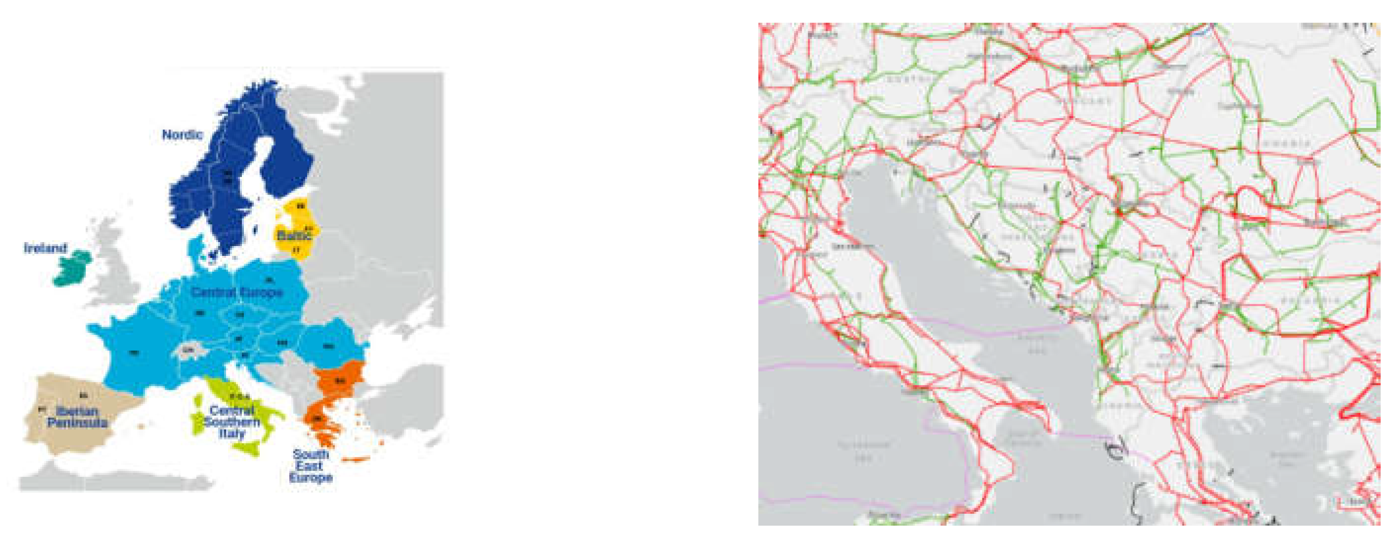
Figure 5.
Time series of hourly spot prices of all markets for the period of 1st January 2022 to 4 October 2024, with quarter boundaries, and values of price spikes at specific dates.
Figure 5.
Time series of hourly spot prices of all markets for the period of 1st January 2022 to 4 October 2024, with quarter boundaries, and values of price spikes at specific dates.
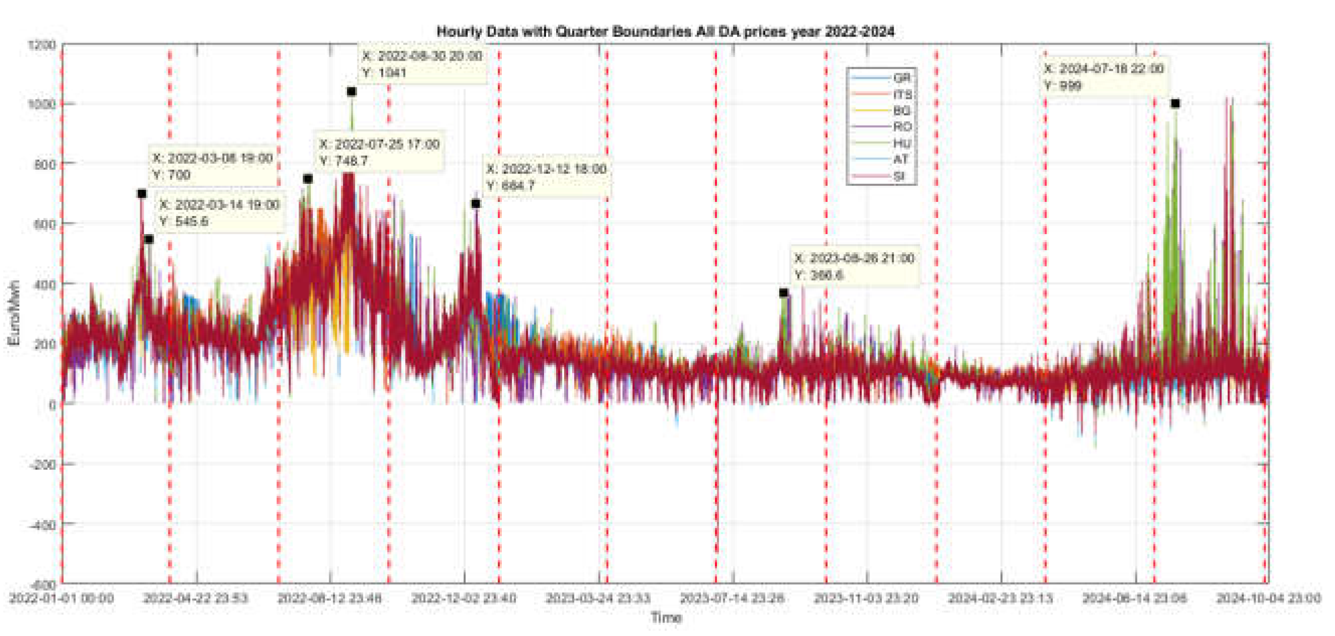
Figure 6.
Time series of Greek DA hourly spot prices for the entire period of 1st January 2022 to 4 October 2024, with quarter boundaries, and values of price spikes at specific dates. On 4th September 2024, at 21:00, the electricity spot hourly Greek price reached 942 Euro/Mwh.
Figure 6.
Time series of Greek DA hourly spot prices for the entire period of 1st January 2022 to 4 October 2024, with quarter boundaries, and values of price spikes at specific dates. On 4th September 2024, at 21:00, the electricity spot hourly Greek price reached 942 Euro/Mwh.
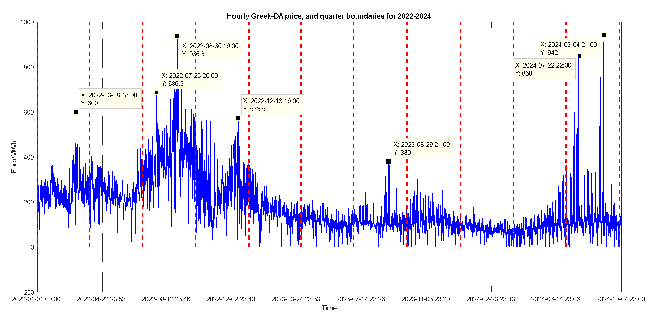
Table 3.
Shows the data set of all fundamental variables considered in our work, collected for each of the seven electricity markets. Descriptive statistics for the hourly spot prices, for each market, are given in Table 4, Table 5, Table 6, and Table 7 (for each separate year and for the entire period 2022-24, respectively). List of all sixty-seven (67) fundamental variables considered in our work, for all electricity markets. In bold letters, the DA spot prices of the markets under analysis.
| Node (Variable) | Name | Description | Unit |
|---|---|---|---|
| 1 | AT_DA_price | DA Electricity price, Austria | Euro/MWh |
| 2 | AT_actTotal_Load | Actual Total Load, Austria | MW |
| 3 | AT_foreTotal_Load | Forecasted Total Load, Austria | MW |
| 4 | AT_actGas | Gas power production, Austria | MW |
| 5 | AT_Solar_Fct | Solar forecst. Power product. , Austria | MW |
| 6 | AT_Hydro_Actual | Hydro Power Forecasted, Austria | MW |
| 7 | BG_DA_price | DA Electricity price, Bulgaria | Euro/MWh |
| 8 | BG_actTotal_Load | Actual Total Load, Bulgaria | MW |
| 9 | BG_foreTotal_Load | Forecasted Total Load, Bulgaria | MW |
| 10 | BG_actGas | Gas power production, Bulgaria | MW |
| 11 | BG_Wind_Fct | Wind forecast generated power, Bulgaria | MW |
| 12 | BG_Solar_Fct | Solar forecast. Power product., Bulgaria | MW |
| 13 | BG_Hydro_Actual | Hydro Power production, actual, Bulgaria | MW |
| 14 | BG_actual_Lignite | Lignite act power production, Bulgaria | MW |
| 15 | GR_DA_price | DA Electricity price, Greece | Euro/MWh |
| 16 | GR_actTotal_Load | Actual Total Load, Greece | MW |
| 17 | GR_foreTotal_Load | Forecasted Total Load, Greece | MW |
| 18 | GR_actGas | Gas power production, Greece | MW |
| 19 | GR_Wind_Fct | Wind forecast generated power, Greece | MW |
| 20 | GR_Solar_Fct | Solar forecast. Power product., Greece | MW |
| 21 | GR_Hydro_Actual | Hydro Power production, actual, Greece | MW |
| 22 | GR_Hydro_Storage_Actual | Hydro Power act consumption, Greece | MW |
| 23 | GR_actual_Lignite | Lignite act power production, Greece | MW |
| 24 | HU_DA_price | DA Electricity price, Hungary | Euro/MWh |
| 25 | HU_actTotal_Load | Actual Total Load, Hungary | MW |
| 26 | HU_foreTotal_Load | Forecasted Total Load, Hungary | MW |
| 27 | HU_actGas | Gas act.power production, Hungary | MW |
| 28 | HU_Wind_Fct | Wind forecast generated power, Hungary | MW |
| 29 | HU_Solar_Fct | Solar forecast. Power product., Hungary | MW |
| 30 | HU_Hydro_Actual | Hydro Power production, actual, Hungary | MW |
| 31 | HU_actual_Lignite | Lignite act power production, Hungary | MW |
| 32 | ITS_DA_price | DA Electricity price, Italy (South) | Euro/MWh |
| 33 | IT_actTotal_Load | Actual Total Load, Italy | MW |
| 34 | IT_foreTotal_Load | Forecasted Total Load, Italy | MW |
| 35 | IT_actGas | Gas power production, Italy | MW |
| 36 | IT_Wind_Fct | Wind forecast generated power, Italia | MW |
| 37 | IT_Solar_Fct | Solar forecast. Power production., Italia | MW |
| 38 | IT_Hydro_Actual | Hydro Power production, actual, Italia | MW |
| 39 | RO_DA_price | DA Electricity price, Romania | Euro/MWh |
| 40 | RO_actTotal_Load | Actual Total Load, Romania | MW |
| 41 | RO_foreTotal_Load | Forecasted Total Load, Romania | MW |
| 42 | RO_actGas | Gas power production, Romania | MW |
| 43 | RO_Wind_Fct | Wind forecast generated power, Romania | MW |
| 44 | RO_Solar_Fct | Solar forecast. Power product., Romania | MW |
| 45 | RO_Hydro_Actual | Hydro Power production, actual, Romania | MW |
| 46 | RO_actual_Lignite | Lignite act. power production, Romania | MW |
| 47 | SI_DA_price | DA Electricity price, Slovenia | Euro/MWh |
| 48 | SI_actTotal_Load | Actual Total Load, Slovenia | MW |
| 49 | SI_foreTotal_Load | Forecasted Total Load, Slovenia | MW |
| 50 | SI_actGas | Gas power production, Slovenia | MW |
| 51 | SI_Solar_Fct | Solar forecast. Power product., Slovenia | MW |
| 52 | SI_Hydro_Actual | Hydro Power production, actual, Slovenia | MW |
| 53 | SI_actual_Lignite | Lignite act power production, Slovenia | MW |
| 54 | GR_BG | Cross Border Transfer, GR-BG | MW |
| 55 | BG_GR | Cross Border Transfer, BG-GR | MW |
| 56 | IT_GR | Cross Border Transfer, IT-GR | MW |
| 57 | GR_IT | Cross Border Transfer, GR-IT | MW |
| 58 | RO_BG | Cross Border Transfer, RO-BG | MW |
| 59 | BG_RO | Cross Border Transfer, BG-RO | MW |
| 60 | SI_IT | Cross Border Transfer, SI-IT | MW |
| 61 | IT_SI | Cross Border Transfer, IT-SI | MW |
| 62 | AT-CH | Cross Border Transfer, AT-CH | MW |
| 63 | AT-CZ | Cross Border Transfer, AT-CZ | MW |
| 64 | AT-DELU | Cross Border Transfer, AT-DELU (Austria to Germany-Luxembourg) | MW |
| 65 | AT-ITNorth | Cross Border Transfer, AT-ITNorth | MW |
| 66 | AT-SI | Cross Border Transfer, AT-SI | MW |
| 67 | AT-HU | Cross Border Transfer, AT-HU | MW |
Table 4.
Descriptive statistics of hourly spot prices, for all markets, 2022-4th October 2024.
| 2022-Oct.2024 | |||||||
|---|---|---|---|---|---|---|---|
| Statistics | HU | RO | BG | GR | ITSouth | SI | AT |
| min | -500.0 | -106.30 | -45.00 | -1.02 | 0.00 | -500.00 | -500.00 |
| max | 1047.10 | 1021.60 | 950.00 | 942.00 | 870.00 | 1023.00 | 919.60 |
| mean | 161.89 | 159.40 | 154.75 | 170.61 | 180.85 | 159.71 | 151.06 |
| median | 120.96 | 119.74 | 119.28 | 130.63 | 134.06 | 117.90 | 111.30 |
| mode | 0.0 | 0.0 | 0.0 | 100 | 100 | 0.0 | 0.0 |
| Std | 128.53 | 128.13 | 119.10 | 117.57 | 120.71 | 126.31 | 122.89 |
| prctile25 | 84.18 | 83.13 | 83.09 | 92.77 | 104.08 | 82.86 | 78.46 |
| prctile75 | 204.15 | 200.63 | 197.51 | 223.07 | 220.00 | 203.50 | 189.10 |
| iqr | 119.97 | 117.50 | 114.42 | 130.30 | 115.92 | 120.64 | 110.64 |
Table 5.
Descriptive statistics of hourly spot prices, for all markets, 2022.
| 2022 | |||||||
|---|---|---|---|---|---|---|---|
| Statistics | HU | RO | BG | GR | ITSouth | SI | AT |
| min | 0.0 | 0.0 | 0.0 | -0.01 | 0.0 | 0.0 | 0.0 |
| max | 1047.10 | 964.20 | 936.30 | 936.30 | 870.00 | 879.30 | 919.60 |
| mean | 271.62 | 265.26 | 253.20 | 279.86 | 295.77 | 274.43 | 261.36 |
| median | 237.20 | 232.58 | 225.08 | 249.28 | 257.23 | 240.01 | 224.00 |
| mode | 138.41 | 138.41 | 138.41 | 200.00 | 650.00 | 220.00 | 190.00 |
| Std | 139.88 | 142.95 | 131.20 | 116.10 | 131.03 | 137.00 | 138.47 |
| prctile25 | 178.25 | 165.31 | 163.27 | 206.89 | 206.43 | 185.03 | 169.09 |
| prctile75 | 345.26 | 342.15 | 320.14 | 339.31 | 370.00 | 343.24 | 336.98 |
| iqr | 167.00 | 176.84 | 156.86 | 132.42 | 163.56 | 164.20 | 167.88 |
Table 6.
Descriptive statistics of hourly spot prices, for all markets, 2023.
| 2023 | |||||||
|---|---|---|---|---|---|---|---|
| Statistics | HU | RO | BG | GR | ITSouth | SI | AT |
| min | -500.0 | -23.18 | -1.10 | 0.0 | 0.0 | -500.0 | -500.0 |
| max | 437.47 |
436.89 | 400.00 | 383.82 | 298.20 | 426.18 | 437.47 |
| mean | 106.79 | 103.71 | 103.82 | 119.09 | 125.03 | 104.30 | 102.11 |
| median | 104.48 |
102.72 | 102.74 | 112.47 | 120.94 | 103.38 | 101.91 |
| mode | 0.0 | 122 | 122 | 100 | 100 | 120 | 0.0 |
| Std | 48.43 | 50.78 | 50.33 | 50.18 | 37.69 | 45.33 | 44.40 |
| prctile25 | 83.75 | 79.26 | 79.20 | 93.00 | 103.47 | 83.21 | 82.09 |
| prctile75 | 133.56 | 132.56 | 132.54 | 141.33 | 145.30 | 130.95 | 128.84 |
| iqr | 49.81 | 53.30 | 53.34 | 48.33 |
41.83 | 47.74 | 46.75 |
Table 7.
Descriptive statistics of hourly spot prices, for all markets, 01-01-2024 to 4th October 2024.
Table 7.
Descriptive statistics of hourly spot prices, for all markets, 01-01-2024 to 4th October 2024.
| 2024 (up to 4th October) | |||||||
|---|---|---|---|---|---|---|---|
| Statistics | HU | RO | BG | GR | ITSouth | SI | AT |
| min | -149.98 | -106.36 | -45.00 | -1.02 | 0.0 | -105.88 | -426.42 |
| max | 999.0 | 1021.6 | 950.00 | 942.0 | 252.1 | 1022.3 | 555.7 |
| mean | 90.15 | 93.53 | 92.37 | 94.79 | 103.24 | 81.85 | 70.48 |
| median | 81.85 | 85.00 | 85.00 | 88.67 | 102.84 | 79.72 | 74.21 |
| mode | 0.0 | 0.0 | 0.0 | 0.04 | 100.0 | 0.0 | 0.0 |
| Std | 78.91 | 78.66 | 74.06 | 64.93 | 31.22 | 56.02 | 37.19 |
| prctile25 | 60.49 | 61.65 | 61.42 | 69.53 | 88.84 | 58.90 | 55.13 |
| prctile75 | 104.98 | 108.01 | 107.49 | 108.11 | 115.59 | 101.82 | 91.20 |
| iqr | 44.49 | 46.35 | 46.06 | 38.58 | 26.75 | 42.91 | 36.07 |
4.1. Boxplots, Aggregated and Hourly-Wised Summary Statistics of Spot Prices
The boxplot comparison of hourly electricity prices across the seven markets reveals notable differences in both price levels and variability. Figure 7 and Figure 8 show, for comparison purposes, the boxplots of the distribution of AT and RO DA prices, hourly-wise i.e. for each separate hour H1 to H24. The boxplots of the rest of the markets are given in Supplementary material D. The same information, quantitatively, as well as other descriptive statistics, is provided in Table A1, Table A2, Table A3, Table A4, Table A5, Table A6 and Table A7, of Supplementary material A. From the figures we see that, for the price levels, Romania (RO) shows consistently higher spot prices than Austria (AT) across almost all hours. The median prices in Romania are around 200–300 EUR/MWh, while Austria's median prices mostly range between 100–200 EUR/MWh. Regarding volatility and outliers, Romania exhibits greater price volatility, indicated by wider interquartile ranges (IQRs), a larger number of extreme outliers (red pluses), often surpassing 800–1000 EUR/MWh, while Austria also shows outliers but with lower frequency and magnitude compared to Romania. For the daily hourly trends, AT’s prices are relatively stable throughout the day, and slight increases in the morning (8–11) and evening (18–21) hours, reflecting typical demand patterns, and finally price distribution is narrower, suggesting a more stable market. RO’s prices tend to spike during evening hours (19–22), both in terms of median and outliers. Morning hours (7–10) also show noticeable increases in median price and spread, and prices are lowest and least volatile between 1–5 AM, consistent with low demand. Now, regarding negative prices, Austria exhibits occasional negative prices, especially in the afternoon hours (13–17), a fact that could be due to high renewable (e.g., solar) generation exceeding demand, grid constraints or export limitations. Romania, in contrast, does not display negative prices, suggesting tighter supply conditions or less flexible generation mix, and possibly lower penetration of renewables or less dynamic market adjustments. Table 8 below gives a summary of the comments above.
Table 9 presents summary statistics across the entire datasets (not just by hour) (we have computed mean, median, standard deviation (St.dev.), interquartile range (IQR) etc., per market, aggregating all 24 hours. This gives us a general picture of volatility and price level without the hourly resolution. The indicators (statistics) (average daily price, standard deviation, average daily peak-of-peak spread, skewness and kurtosis and frequency of extreme prices, e.g. > 90th percentile) help us rank the markets more broadly, without dissecting hour-by-hour details (which are, however. shown in Figure 4, Figure 5, Figure 6, Figure 7, Figure 8, Figure 9 and Figure 10 and Table A1, Table A2, Table A3, Table A4, Table A5, Table A6 and Table A7 of Supplement A). The note at the bottom of Table 7 explains the indicators shown.
Thus, based on Table 9, the Italian and Greek markets (ITS and GR) exhibit the highest mean and median prices, suggesting a generally more expensive electricity supply, while Slovenian and Austrian markets (SI and AT) have the lowest medians (117.9 and 111.3 respectively), indicating more affordable rates. Greek market displays the wider interquartile range (IQR=120.6), reflecting greater variability in hourly prices and potentially higher market volatility (even though has the lowest aggregated st.dev). In contrast, AT and BG markets have a relatively narrow IQR, pointing to more stable and predictable pricing. Romanian and Bulgarian markets have the largest Peak-Off-Peak (PoP) spreads (95.3 and 94.1) followed by Hungarian and Greek markets (86.1 and 76.43). The largest CV (coefficient of variation, a volatility measure) is presented by TA and RO markets, followed by HU and GR markets. Additionally, skewed distributions in markets TA, BG, HU, ITS and RO hint at asymmetric pricing behavior, showing a tendency for upward price spikes. The table shows no differences between the markets for the frequency of extreme points, and HU exhibits the highest price, followed by SI and RO markets. From Table 10 we observe that the Greek and Italian markets have the highest total number of hourly price outliers.
4.2. Correlation Analysis of All Raw DATA, 2022-Oct2024.
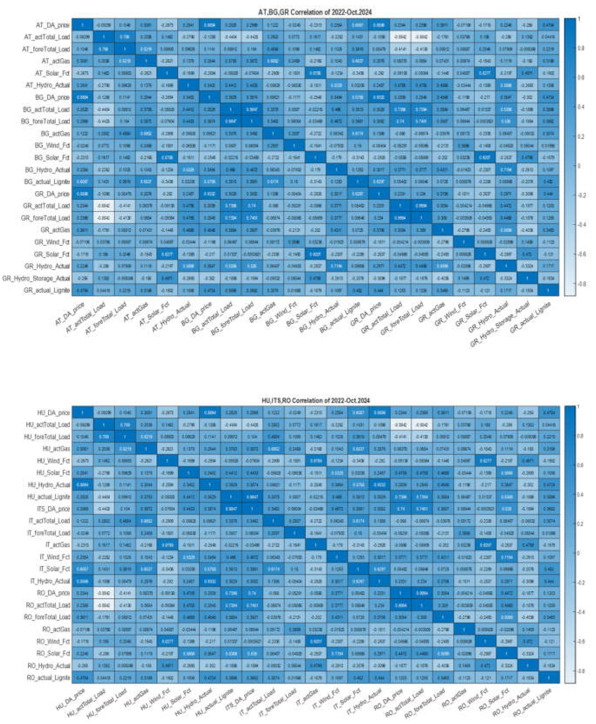
Even though correlation analysis is not capable of revealing any causalities, profound or hidden, its result can serve as a useful, albeit rough guide of the ‘interactions’ between the variables involved. We use correlation analysis (Figure 9a–d) to ‘detect’: a) strong regional spot price interactions, b) price-fuel correlations, c) North-South correlation gradient (strength), d) cluster of markets and finally e) the role of local fuels. High correlations between neighboring countries' Day-Ahead (DA) prices (e.g., AT-DA-price, HU-DA-price, SI-DA-price) suggest significant market coupling or shared supply-demand fundamentals. These strong correlations may reflect cross-border electricity trade, similar weather conditions or economic patterns, and coordinated market operations within the EU internal electricity market. Regarding price-fuel correlations, we observe that GR-Gas, AT-Gas, HU-Gas, and SL-Gas have medium to small positive correlations with DA prices in their respective countries, while this fact is not observed in BG, IT and RO markets. This results in natural gas being a relatively marginal fuel, especially during price-setting hours, highlighting the influence, to some degree, of gas prices on electricity pricing in these markets. Now, as far as the strength or gradient of correlations, from north to south markets, we observe a decrease in correlation strength between prices from Core CCR (AT, HU, SI, RO) to SEE CCR markets (GR, IT). For example, the average spot prices correlation between AT and HU, SI and RO markets, is higher than in AT and GR, BG markets (0.94 and 0.86 respectively). The same is observed between the mean correlation of prices of HU, SL and RO markets, with the mean value between HU and GR markets (0.965 and 0.915). This could indicate transmission bottlenecks, different generation mixes (e.g., higher renewable share in some markets), or regulatory or market structure differences. The figures show also clustered Markets countries like AT, HU, SI, and RO that form a highly correlated cluster, indicating a tightly interconnected sub-region, while GR and IT are more loosely connected, possibly due to their geographical positioning and more, in general, isolated grid conditions. For the role of local fuels play, we observe that hydro and lignite generation in BG and GR markets are only locally correlated with their own DA prices, which implies a local dependency on these two fuels for power generation. The two markets show similar local dependency of their own prices on their RES (wind and solar generations).
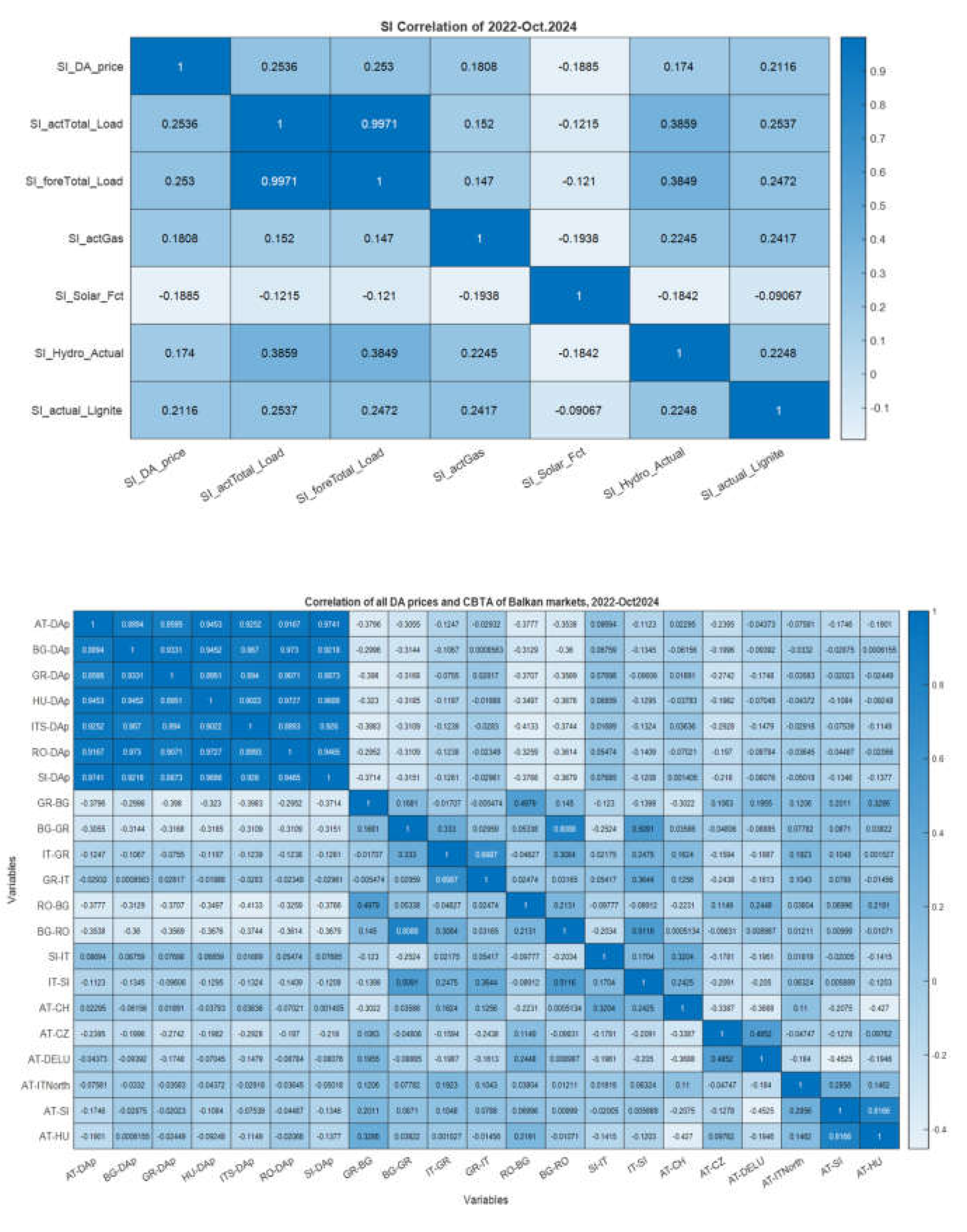
We observe also that the cross-border transfer availabilities (CBTAs) RO-BG (between Romania and Bulgaria), BG-RO, GR-BG, and BG-GR exhibit the largest, negative correlations with the spot prices. Instead of trying to explain these findings, we refer to Section 7.3 where we present the results of rolling volatility spillover of spot prices and CBTAs, between all pairs of markets. More specifically, we have computed the correlations of the rolling volatility curves of both spot prices and CBTAs, of all markets, and have analyzed their volatility spillover from one market to another, thus enhancing further the causality structure learning findings of Section 7.1 (MB and LCSL results).
Figure 9.
a: Heat map of all possible correlations between pairs of AT, BG, GR markets’ fundamental parameters, excluding CBTA. b: Heat map of all correlations between pairs of HU, ITS, RO markets’ fundamental parameters, excluding CBTA. c: Heat map of all correlations between pairs of SI market’s fundamental parameters, excluding CBTA. d: Heat map of correlations between pairs of all DA prices and Cross Border Transfer (CBT) availability.
5. Methodology
In Section 5.1 we provide a short review for Global, Local Causal structure learning, and Markov Blanket learning, emphasizing their differences and the fields they are applied, although we do not use Global causal structure learning in the present work. Section 5.2–5.4 then present the necessary mathematical background (definitions and key propositions without proofs), with emphasis on Markov Blanket learning, and finally Section 5.5–5.8 provide information on the practical aspects of the applied algorithms.
5.1. The Difference Between Global, Local Causal Structure Learning, and Markov Blanket Learning
Causal structure learning involves discovering the causal relationships among variables in a dataset. The three main approaches—Global Causal Structure Learning (GCSL), Local Causal Structure Learning (LCSL), and Markov Blanket Learning (MBL) differ in their scope and methodology. In the GCSL, the goal is to learn the entire causal graph over all variables in the dataset, using various approaches such as constraint-based, score-based, or hybrid methods to infer the global causal structure. Constraint-based method uses conditional independence tests (e.g., Parent Child -PC- algorithm, FCI), while the score-based one optimizes a scoring function (e.g., BIC, Bayesian scores) over possible graphs (e.g., GES). Finally, the hybrid method combines both approaches (e.g., Max-Min Hill-Climbing, MMHC). The advantages of GCLS are the fact that it provides a complete causal structure (it provides ‘the big picture’ of the problem under analysis, and it can infer direct and indirect causal effects. However, it is computationally expensive, especially for high-dimensional data, and it requires strong assumptions (e.g., causal sufficiency, faithfulness). This is the reason (as well as the advantages of LCSL listed below) we do not use this method in this work. The transition from local to global learning plays an essential role in Bayesian network (BN) structure learning. Mainstream algorithms for this type of learning were based on first constructing the skeleton of a DAG (directed acyclic graph) by learning the MB (Markov blanket) or PC (parents and children) of each variable in a data set and then orienting edges in the skeleton. Since it requires expensive computational resources (especially with a large-sized BN, resulting in inefficient local-to-global learning algorithms), [6] developed an efficient local-to-global learning approach using feature selection, using the well-known Minimum-Redundancy and Maximum-Relevance (MRMR) feature selection approach for learning a PC set of a variable, and proposed the efficient F2SL (feature selection-based structure learning) approach to local-to-global BN structure learning, the algorithm adopted in our preset work.
One the opposite, in LCSL the goal is to learn causal relationships for a subset of variables (e.g., the most crucial variable around a target variable). We focused on this method, since our main target is to detect the most relevant factors that shape the dynamics (especially the surge) of spot prices target variables. The most crucial variables coincide with the set of members detected in the MB. LCSL identifies MB’s members direct causes and effects without reconstructing the entire causal graph, using methods as local constraint-based methods (e.g., HITON, Grow-Shrink, see Table 11), and local score-based methods. Advantages of this learning method include that it is more scalable than global learning, and focuses on relevant variables, therefore reducing noise. However, LCSL does not capture the full causal structure (across all European interconnected markets) and may miss indirect causal effects, however avoiding both these ‘defects’, is beyond the purpose of our analysis.
We applied Local causal structure learning (LCSL) in our dataset to discover and distinguish the direct causes and direct effects of all seven DA spot prices, the chosen target variables. Since the mainstream LCSL algorithms need to perform an exhaustive subset search within the currently selected variables for PC (i.e., parents and children) discovery, to speed up and make the process more efficient, several algorithms have been developed. Examples are the work of [19], proposing the LCS FS model and the Causal Markov Blanket, CMB [18] is the algorithm adopted in our study.
In the MB learning, the goal is to identify the Markov Blanket of a target variable, which consists of Parents (direct causes), Children (direct effects), and Spouses (other parents of the target’s children). It uses conditional independence tests or local structure learning to identify the minimal set of variables that render the target variable conditionally independent from all others. A plethora of methods exist, such as HITON-MB, IAMB, Fast-IAMB, PCMB, InterIAMBnPC (see also Table 8). This learning approach is efficient for feature selection and reduces dimensionality while preserving relevant information. However, it does not provide a full causal graph and is sensitive to sample size and independence test accuracy. Therefore, we can use Global Learning when the entire causal structure is needed (e.g., causal discovery), Local Learning when only a subset of causal relationships is relevant and Markov Blanket Learning when feature selection is needed (e.g., as in machine learning, predictive modeling). In our present work we have adopted the combination of MB and LCSL and the InterIAMBnPC algorithm [32] for MB learning.
In the application of Markov Blanket Learning in detecting causalities in electricity markets the main goal, as already mentioned, is the ‘revealing’ of a subset of variables, i.e. Markov Blanket of a target variable (e.g., electricity price in a specific market) consisting of the direct causes (parents) → Fundamental drivers (e.g., demand, supply, weather, fuel prices, interconnector flows, i.e. CBTAs), direct effects (children) → Downstream impacts (e.g., price fluctuations in neighboring markets), and finally spouses (other parents of the target’s children) → Variables that influence price through shared dependencies. Therefore, by identifying the MB of a spot price, we can determine the most relevant factors affecting price fluctuations while filtering out irrelevant variables. MB is particularly useful for feature selection (reducing dimensionality), predictive modeling (improving forecasting), and identifying key influences of price changes (this is the case in our paper). We stress here that MB learning alone does not establish causal direction beyond identifying relevant variables. The challenges with using only MB learning are: a) no explicit causal structure as the learning tell us which variables are important but not necessarily the cause-effect relationships, b) it does not capture indirect effects, since some causes may influence price via intermediate variables, which MB learning might miss, and c) the method does not consider temporal causality, since spot prices are dynamic and evolve over time, and MB learning typically works on static datasets. To overcome these problems and properly discover causal relationships, as we have pointed out, we combine MBL with LCSL and mainstream time series analysis, as the rolling volatility of spot prices and CBTAs, to capture the volatility spillover effects due to interaction of the markets. The steps of our workflow are described as follows:
Step 1: MB Learning (Feature Selection). We used the algorithm IAMB, to identify the most relevant fundamental variables affecting DA electricity prices, thus reducing further the dimensionality of the dataset and focusing only on key drivers.
Step 2: Causal Discovery on the MB Selected Variables, we applied LCSL (CMB algorithm) to the wholesale DA price variables to determine direct causal relationships.
Step 3: We validated the results by using the results of volatility spillover as well as consulting experts in the electricity markets field working in the Greek TSO and other European institutions (see affiliations of authors), to ensure that our findings align with real energy market dynamics (domain knowledge).
5.2. A Short Mathematical Background in Bayesian network (BN), Markov blanket (MB) and Causal Feature Selection (CFS)
We provide here the necessary, short background theoretical information (notation and definitions etc.), based on the works of [6,20] which describe in a rigorous mathematical approach all the theoretical basis (all related theorems and their proofs).
We symbolize with C our Target Variable (TV) (or Class attribute, CA) of interest. Let φ represent the distinct TV values (or labels), as c={ , and the set of all distinct features. Let also that D is a training dataset, D=, with the number of instances, the i-th instance i.e. a n-dimensional vector defined on F, and a label of the TV associated with . To facilitate our presentation, let the set of all variables under consideration in our analysis, where and C . Let V \ indicate the set V \{ }, that is, all features excluding , ∀∈V. To consider conditionality, let use ╨ |S are conditionally independent given S, and , and the expression (not ╨) |S, to denote that is conditionally dependent on given S.
Definition 1 (Conditional Independence). Two distinct variables ∈V are said to be conditionally independent given a subset of variables S ⊆V \ { } (i.e., ╨ |S), if and only if P (|S) = P( |S)P( |S). Otherwise, are conditionally dependent given S, (not ╨) |S.
5.3. Bayesian Network, Markov Blanket, and Causal Feature Selection
We provide basic knowledge at this point associated with causal feature selection (CFS), including the basics of BN, MB, and why we choose causal feature selection. Suppose that P (V) is the joint probability distribution over the set of all variables V, and G = (V, E) represents a directed acyclic graph (DAG) having nodes V and edges E, where an edge represents the direct dependence relationship between two variables.
In a DAG, symbolizes that is a parent of and is a child of .
Definition 2 [20]. The triplet V, G, P(V)is called a BN, if the Markov condition as defined below (definition 3) is valid:
Definition 3 (Markov Condition) [20]. For a DAG G, the Markov condition holds in G, if and only if, every node of G is independent of any subset of its non-descendants conditioned on its parents. Thus, the joint probability over a set of variables V is encoded by a BN which decomposes P (V) into the product of the conditional probability distributions of the variables given their parents in G.
Let () be the set of parents of in G. Then, P(V) can be written as
In this paper, we consider a CBN, a BN in which an edge indicates that is a direct cause of [20,21]. In the definition 4 below, we give the key concepts and assumptions associated with BNs and MBs.
Definition 4 (Faithfulness) [20]. Suppose that a BN <V, G, P (V)>, then G is faithful to P(V) if and only if every conditional independence present in P is entailed by G and the Markov condition. P(V) is faithful if and only if G is faithful to P (V).
Definition 5 (Causal Sufficiency) [20]. Causal sufficiency assumes that any common cause of two or more variables in V is also in V.
Definition 6 (d-Separation) [20]. In a path πof a DAG G, and are said to be blocked by a set of nodes S ⊂V, if and only if: (a) π contains a chain
or a fork
such that the middle node is in S, or (b) the path π contains a v-structure
such that S holds and no descendants of are in S. A set S is said to d-separatefrom if and only if S blocks every path from
Theorem 1 [20,21]. Given a BN <V,G, P (V )>, under the faithfulness assumption, d-separation captures all conditional independence relations that are encoded in G, which implies that and in G are d-separated by S ⊂V \{, }, if and only if and are conditionally independent given S in P(V). The theorem concludes the equivalence of conditional independence in data distribution and d-separation in the corresponding DAG, under the assumption of faithfulness.
Definition 7 Markov Blanket (MB). [20]. The Markov Blanket (MB) of a variable in a BN is unique and consists of its parents (direct causes), children (direct effects), and spouses (other parents of the variable’s children), provided that the faithfulness assumption is valid.
The relation between PC in a BN, and how to identify spouses are given by proposition 1 and 2 respectively and are the basis of designing CFS algorithms.
Proposition 1 [21]. In a BN, there is an edge between the pair of nodes and , if and only if they are dependent (i.e. (not ╨) |S), for all S ⊆V \ { , }.
Proposition 2 [21]. In a BN, assuming that is adjacent to , is adjacent to , and is not adjacent to (e.g., → ←), if ∀S ⊆V \ { , }, ╨ |S) and (not ╨) |S∪{ is a spouse of .
The cornerstone of causal and non-causal feature selection is the concept of Mutual Information (MI), introduced initially in machine learning by [22] and later by [23,24], and used then as an additional concept in explaining feature relevance, in non-causal FS [25]. The conditional MI between X and Y given another feature Z is given by:
It is based on the concept of Sannon’s entropy:
of a variable X, and on the conditional entropy of X after observing the values of Y
In equations (3) ana (4), P(x) is the prior probability of X=x (the value x that the variable X takes) and similarly P(Y) is the posterior probability of Y=y, in the context of Bayes Rule, so the MI between X and Y is
Using (2), then in the context of non-causal FS, a feature is strongly relevant to C if and only if I(.
5.4. The Objective Function of Optimal Feature Selection Problem, Based on the MI Concept
The problem of finding a subset , given a dataset D containing C and F, in a feature selection context is formulated as follows
i.e. try to find a subset of features that maximizes the conditional probability of C. Equation (6), using equation (2) is written finally as
It is shown, in the literature provided, that the feature set S∗ defined in Equation (7) is the set of features that leads to the minimal Bayes error rate. Recently, [26] has shown that for a given classification problem, the minimum classification error attainable, by any classifier, is called its Bayes error rate. In this work we adopt the approach of [25] in choosing the Bayes error rate for justifying Equation (7) since, according to the associated literature, this error is the tightest possible classifier-independent lower-bound, since it depends only on the predictor features and the Target variable (class attribute). In setting the lower and upper bounds on the Bayes error rate, [27,28,29] have finally made the connection of the Shannon conditional entropy [30] to the Bayes error rate, a crucial step in rigorously formulating CFS approach in ML.
In general, Feature selection (FS) is used in model building as well as data understanding and is a process of identifying a subset of features (predictor variables) from the original set of features. FS is more pressing now, in the era of big data, since the handling of ‘inherently ubiquitous’ high-dimensional datasets is very difficult. FS has become the cornerstone behind any efficient classification model. There is a plethora of FS methods that fall into three categories: a) Filter, b) Wrapper and c) embedded methods. The two last methods are classifier dependent while filter methods are classifier or prediction model independent.
Strongly relevant features, weakly relevant features and irrelevant features are the types of features that characterize the relevance of given predictors with a class attribute (also called target variable) [31]. The aim of the FS is to identify the strongly relevant features of the Target variable, and this is achieved by first ranking the features according to their relevance to the Target variable and then by using an iterative process, selecting for inclusion the most relevant features [32].
In this paper, the method used for MB (the CMB) uses an emerging, very efficient FS filter method in identifying a Markov blanket (MB) of the class attribute or Target variable [33], a concept invented by Pearl [20] in the framework of Bayesian network (BN). The components of the MB of a variable are of its parents (direct causes), children (direct effects), and spouses (other parents of this variable’s children). A medical example of using this method is given in figure SB1, in Supplementary Material B.
The LCS has the advantage that causality is connected to the capacity of the related models to generate better and more interpretable predictions. The MB (filter) selection approach is also called causal feature selection (CFS) [6] (a term also used in this work) to better understand the mechanisms behind the wholesale (spot) electricity prices of the SEE markets, and more specifically the causes that are behind their ‘extreme’ values (strong price disparities). CFS approach is an approach that has been shown to be theoretically optimal, in comparison with a non-causal FS.
5.5. The Markov Blanket (MB), a Tool for Causal Feature Selection to Reveal the Strongest Factors Influencing DA Electricity Prices
The Markov Blanket, as defined previously (definition 7), a concept from Bayesian networks and the associated probabilistic graphical models, is a powerful tool able to identify the set of variables that shield a target variable from the influence of all others, a tool particularly useful in causal feature selection. We explain here how it is used in the CFS of the DA (spot) electricity price, our Target variable, symbolized as TV-SpotElectP. From definition 7, the components of the MB of this variable will be: the Parents i.e. Variables that directly cause the dynamics of TV-SpotElectP, the Children i.e. variables directly caused (affected) by TV-SpotElectP, and finally the Co-parents (Spouses) i.e. other variables that cause (affect) TV-SpotElectP’s children. Together, these components determine the smallest set that makes TV-SpotElectP conditionally independent of all other variables in the system. The steps followed in using MB for feature selection are a) building a probabilistic Graphical Model i.e. using data to construct a probabilistic graphical model, such as a Bayesian network, that encodes the conditional dependencies between variables, b) identify the Markov Blanket i.e. applying a variety of algorithms (see Table 8) to identify the Markov Blanket of the target variable, which will include the most causally relevant features for TV-SpotElectP, c) analyzing the Markov Blanket i.e. examining the MB’s that are directly or indirectly causally related to TV-SpotElectP, i.e. the strongest factors influencing target variable (the absence of a variable from the blanket implies it is irrelevant or redundant for predicting our target variable , given the variables in the blanket). We list here some of the advantages of using the MB, namely the causal relevance (since MB focuses on features with causal influence on the target, avoiding spurious correlations), the minimal feature set (Mb identifies the smallest set of variables needed for accurate prediction of target variable), and finally the fact that MB provides interpretable models(by isolating causally relevant factors, it simplifies interpretation of the model). Thus, our paper contributes towards enhancing the limited number of papers in which MB is used in the analysis of energy issues.
5.6. Practical Aspects in Applying the MB CFS Approach to Understand Price Surges in SEE Electricity Markets and a Suggested Workflow.
We describe here the steps we have followed in applying this approach to our work: in step 1 we define our target variable, i.e. the TV-SpotElectP, the wholesale prices. In step 2 we identify candidate variables. We have considered factors potentially influencing price surges, such as: a) Energy Supply Factors: Gas prices, coal prices, renewable energy generation, and imports/exports (Cross-border Transfer availability, CBTA), b) Load Factors: actual and forecasted load, of each market, c) Market Dynamics: Market coupling approaches with neighboring countries, via CBTA (see Section 3), d) Policy Factors: we have considered relevant publicly available information, for each country, policies such as subsidies, taxes, and EU Emissions Trading System (ETS) costs, only in cases that we think can support interpreting our models results. Then, in step 3, we construct a Probabilistic Graphical Model. We use data to construct a Bayesian network or a similar probabilistic graphical model, if this is possible, that represents conditional dependencies between variables in each market, based on its assumptions, and in step 4, we ‘discover’ the Markov Blanket, by using a plethora of algorithms (see Table 8), i.e. we identify the MB for a given target variable. This will include Parents (Variables directly causing price surges), Children (Variables influenced by price surges), and Co-parents (Variables that jointly influence the children of price surges). We interpret results, in the final stage: Variables in the Markov Blanket are the strongest factors influencing electricity price surges, for example, if gas prices, renewable generation, and market coupling are in the Markov Blanket, these are causally relevant, while other variables are conditionally independent given the blanket. Finally, we use LCSL approach to ‘capture’ the causality directions between the variables identified by MB. Figure 10 presents the work flow we followed in using CFS MB approach to energy market analysis.
Figure 10.
The workflow in using the CFS MB approach detecting the most crucial predictors (features) that affect hourly spot prices in the DA electricity markets analyzed.
Figure 10.
The workflow in using the CFS MB approach detecting the most crucial predictors (features) that affect hourly spot prices in the DA electricity markets analyzed.
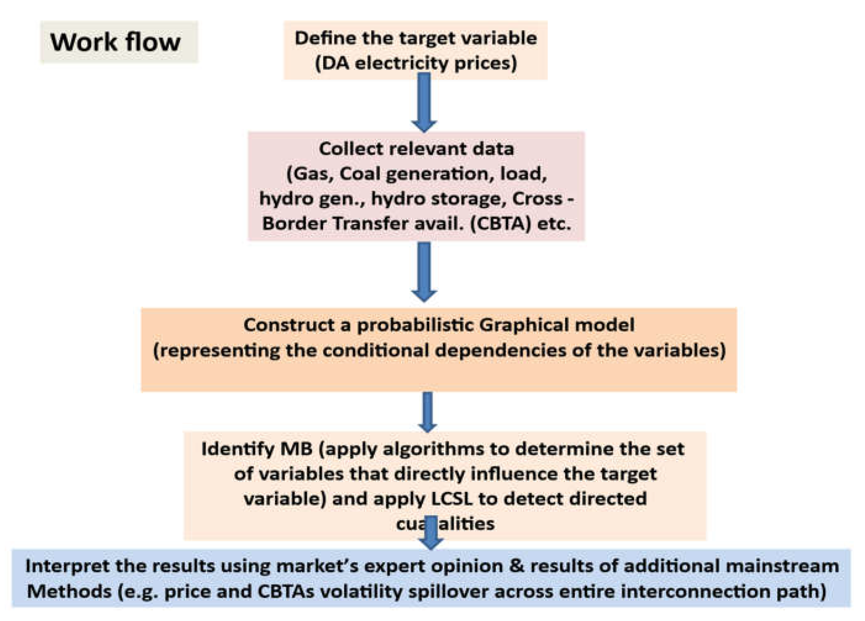
The steps in the workflow are:
- Define the Target Variable: in our case, electricity price surges in all seven markets.
- Collect Relevant Data: Gather data on potentially influencing factors, such as fuel prices, demand and supply metrics, policy changes, and geopolitical events.
- Construct a Probabilistic Graphical Model: Use the collected data to build a model that represents the conditional dependencies between variables.
- Identify the Markov Blanket MB: Apply algorithms to determine the set of variables that directly influence the target variable.
- Use LCSL methodology to identify the direct causalities between the member-variables of the MB
- Interpret the Results: Analyze the identified factors to understand their causal impact on electricity price surges, using results from volatility spillovers, and opinions form the market experts.
5.7. Justification of Using Causal Discovery and Feature Selection Approach Instead of a Typical Regression Model.
At this point, we think that we must provide the reasons for adopting the MB approach instead of other ‘mainstream’ approaches as regression modeling. We list the advantages of the Markov Blanket Approach: first, this method focuses on Causal Relationships: the Markov Blanket isolates variables with a direct or indirect causal impact on price surges, reducing noise from spurious correlations. As an example, if coal (lignite) prices are conditionally independent of price surges given gas prices, the model excludes coal prices as a key factor. Second, the approach defines a Minimal Feature Set: it identifies the smallest set of variables needed to explain the target, leading to simpler, more interpretable models. Third, the approach exhibits Robustness to Multicollinearity: unlike regression, which can struggle with multicollinearity (e.g., between gas prices and renewable generation), the Markov Blanket approach accounts for conditional dependencies. Fourth, it handles Nonlinear and Complex Interactions: Probabilistic graphical models capture nonlinear relationships and interactions between variables, which are common in electricity markets. From our literature review, Table 11 has emerged, summarizing all the previous advantages of MB over a regression approach
Table 11.
Comparison of MB with Regression Approaches.
| Aspect | Markov Blanket | Regression |
|---|---|---|
| Focus | Causal relationships | Statistical associations |
| Feature Selection | Identifies causally relevant variables | May include spurious or redundant variables |
| Handling Multicollinearity | Resolves through conditional independence | Struggles without feature engineering |
| Model Complexity | Produces a minimal set of explanatory variables | Includes all statistically significant variables |
| Interpretability | Provides clear causal explanations | Explains variance but not causality |
| Assumptions | Requires conditional independence assumption | Assumes linearity (in linear regression) |
| Performance in High Dimensions | Effective for sparse causal structures | May be overfit without regularization |
To facilitate reader’s interpretation, we provide below a simple example of a possible indicative result among other possible results described in Section 7. Example: explaining DA price surges in SEE electricity markets by using MB. Let the result of Markov Blanket Approach is as follows: MB Identifies gas prices, renewable generation, and EU ETS costs as causally relevant. The interpretation is that Gas prices directly cause price surges, renewable generation mitigate surges, and ETS costs amplify them. Other variables (e.g., coal prices) are conditionally independent given these factors. In a traditional regression approach the expected result is gas prices, renewable generation, coal prices, and industrial demand are statistically significant predictors. In the interpretation of the result of this method we may be aware that the method may overemphasize the role of coal prices due to multicollinearity with gas prices, leading to less clear causal insights.
Therefore, since our goal is to identify ‘true’ causal drivers of price surges, i.e. a causal inference target, then it is better to prefer the MB Approach. Also, this approach is preferred in the case of Complex Interactions i.e. when relationships between variables are nonlinear or involve interactions (complex inference). Finally, the MB is strongly more effective in causality inference in the case of high-dimensional data, i.e. when dealing with many potential predictors, since the MB simplifies the feature set. Finally, to complete the comparison of MB with regression, regression is preferable when the goal is simply to predict price surges, not explain them, or when linear relationships prevail in the dynamics, i.e. when relationships between variables are linear and well understood, and finally when data size or quality is insufficient for reliable causal discovery. Thus, in conclusion, the MB excels in revealing the strongest causal factors behind electricity price surges, providing a more interpretable and causally grounded analysis compared to regression. While regression is a powerful predictive tool, it is less suited for uncovering causal mechanisms in complex systems like electricity markets.
5.8. Algorithms Associated with Causal Discovery and Feature Selection (CFS) and MB
CFS is the methodology to find the Markov Blanket (MB) of the target variable in a CBN context [34], in which an edge X →Y indicates that X is a direct cause (parent) of Y, and Y is a direct effect (child) of X, therefore the MB of the target variable consists of the parents, children, and the spouses (i.e. other parents of the children), and offers a complete picture around the local causal structure (LCS). Most important, from a statistical point of view, the blanket represents a minimal set of features that makes the target variable statistically independent from all the other features conditioned on the MB [20]. The minimal set of features, determined by MB, is also the optimally found subset for the purpose of classification as well as a holistic interpretation of the predictors that strongly affect the target variable [32].
[35] invented the first sound MB discovery algorithm, GS (Growing-Shrinking) for BN structure learning, that replaced the KS model [36] who were the first to introduce MBs to feature selection, but with the problem of not being able to secure the finding of the actual MB. Another generation of improved algorithms for optimal FS are the Incremental Association-based MB (IAMB) family of algorithms, such as IAMB, inter-IAMB, IAMBnPC [36], and Fast-IAMB [37]. A list of the algorithms for global causal structure FS learning is given in the following Table 12:
Figure 11.
A schematic representation of the Global Causal Structure, Local Causal structure and Markov Blanket.
Figure 11.
A schematic representation of the Global Causal Structure, Local Causal structure and Markov Blanket.
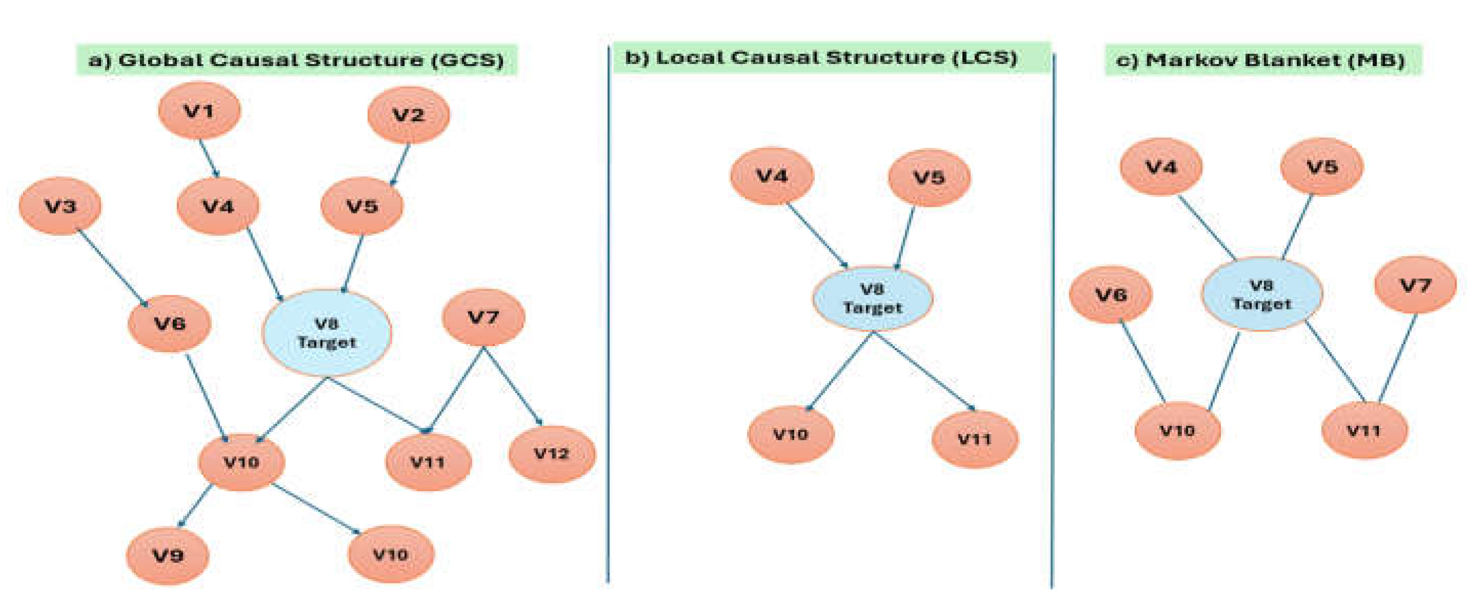
6. Rolling Volatility of DA prices and Their Correlation to ‘Grasp’ Spillover Effects
The spillover of electricity price volatility across 24 countries in the European Union has been recently studied by [38], during the period 2014-2024. Six of the markets analyzed in our paper are included (Bulgaria is missing) in their study, in which the [39,40,41] measure is used to capture the volatility spillover between AT, HU, GR, BG, RO, and IT, and their findings are used here to support our findings. They developed both a static and a dynamic assessment of spillover effects and directional decomposition between individual markets. Their main findings, that are very related to our study, show that a very large amount of the volatility (about 73 percent of the forecast error variation) is explained by cross-variance shares, meaning that only 27 percent can be attributed to shocks within each market, therefore cross-border volatility spillovers dominate the behavior in national electricity markets in Europe, an effect that has increased over time. Instead of using the Diebold-Yilmaz (DY) [39,40,41] approach (our objective in our paper is different), we have computed the rolling volatility (standard deviation) of DA prices of all markets, using a window of 720 hours (a month), as well as the correlations between all pairs of the rolling volatility curves.
We can combine the above correlation information, with several methods like visual cluster maps or a table comparing structural plus weather similarities, or clustering these markets statistically e.g., via a dendrogram (see Figure 24) to capture the clustering processes. Figure 24 shows the dendrogram method of clustering process, that uses K-means extracted features, based on the correlation matrix of the rolling volatility curves of the hourly spot prices and CBTAs of these countries so we can extract conclusions about the price volatility spillover. This is a very important step, since we connect a linear statistical measure, the correlation of rolling volatilities of the most crucial factors identified via nonlinear methods (MB and LCS), with economic and structural reasoning to extract insightful conclusions about how volatility spillovers affect the spot prices surge. Now, a natural question is what do volatility correlation values really tell us? When we correlate rolling volatilities of spot prices, we're essentially measuring how synchronous the “intensity of risk” or price variability is across markets over time—not just price levels, but how similar the volatility dynamics are. Therefore, a) high correlation in volatility indicates co-movement in risk or uncertainty across markets, b) suggests common drivers, such as weather conditions, shared fuel price shocks (e.g., gas prices), interconnected grid events, and finally policy or regulation changes affecting multiple markets. On the other hand, low correlation in volatility means that volatility is idiosyncratic, driven by local factors, like domestic generation mix, internal grid congestion and country-specific demand patterns or weather anomalies. Table 13 summarizes possible interpretations of the high and low correlation of volatilities between two markets.
In case we see low volatility correlation despite interconnection, it may suggest that one market is isolated in volatility terms (e.g., due to internal constraints or pricing mechanisms), market resilience or decoupling—volatility is not transmitting effectively, and finally asymmetric spillovers — one market is a transmitter but the other absorbs differently.
Even though correlation is symmetric, we can try to infer directional spillover tendencies, thus we overlay indicative correlation patterns with structural asymmetries, as in Table 14.
For example, we see that the interconnections BG–RO and GR-BG exhibit high volatility correlation, thus we likely observe volatility co-movement due to weather and grid interconnection, possibly bidirectional spillovers. Similarly, we see that GR volatility is correlated more with BG than with IT, despite physical ties with IT, market coupling with BG dominates volatility transmission. Therefore, our conclusion is that clustered Volatility Patterns ‘resemble’ or somehow ‘coincide’ with volatility Spillover Zones.
The Clustering Tool Dendrogram, in Our Context
A dendrogram (see Figure 21) is a tree-like diagram that shows how electricity markets (based on their volatility correlation similarities) cluster together — from most similar to least one. The dendrogram is useful to us because it helps us group structurally similar markets without relying only on market rules — it’s data-driven, i.e. it can validate or challenge existing market integration assumptions (measured by the interconnectivity level, Section 3). It reveals how volatility spillovers operate naturally, beyond algorithmic models like FBMC, and finally is powerful in highlighting hidden market coupling dynamics or stress-induced decoupling. The Y-axis shows the labels of spot prices and CBTAs. The X-Axis shows the distance or dissimilarity metric we have computed as → Distance = sqrt(2*(1 - correlation)). Therefore, lower distance = higher correlation → more similar volatilities, and higher distance = less correlated → less similar volatilities. Regarding dendrogram’s branches and merging points, the closer two markets merge at the bottom, the more similar they are in terms of volatility behavior, and markets that merge early (at low height) → high correlation of volatility patterns → structurally similar, while markets that only join clusters at higher levels are more volatility divergent.
7. Empirical Results
7.1. Markov Blanket Learning
7.1.1. MB analysis of DA Prices as Target Variable
As already mentioned, Markov Blanket discovery helps reduce the search space by selecting the most relevant variables. We present in Table 14 the results of applying the MB IAMBnPC algorithm on our dataset, choosing as target variable each DA-price, for each year to detect the evolution of the dominant factors (members of the MB) that affect the price over the period of our analysis. Also, in Figures 13a, 13b and 14, we present the annual DAGs for MB results graphically, learned by the IAMBnPC algorithm, setting as target variables the DA prices of the Austrian (AT), Greek (GR) and Italian (IT) markets. Similar figures can be drawn for the other markets but not shown in this report.
For the Austrian DA price, during 2022, we observe in Figure 13a that the set of the MB members consists of the DA prices of the two directly interconnected neighboring markets of HU and SI, as well as Italy’s price (a rather surprising result), and the cross-border transfer availabilities (CBTAs) of Austria with its neighboring Czech, Germany-Luxembourg and Slovenia (AT-CZ, AT-DELU and AT-SI). The AT-SI CBTA is present also in 2023, during which the RO-BG CBTA is also included, together with two Bulgarian power generation variables (Gas and Hydro), the HU and SI spot prices, and the SI hydro generation. Thus, it seems that the RO-BG CBTA has affected the price in HU which in turn has affected the AT price, which is also affected by the SI price. In 2024, we see that AT-DELU and GR-BG CBTAs are in the MB set, together with SI and GR(?) spot prices, AT’s solar and hydro power generations, GR’s hydro power, and IT gas and HU lignite power generations. The presence of AT-DELU CBTA in 2022, 2023 and 2024 indicates the significance of this variable in shaping the dynamics of AT spot price. We point out that the FBMC approach is implemented to optimize the cross-border electricity flows between AT, DELU, SI, HU and RO (Section 3).
In the Greek case (Figure 13b) we observe that nodes (variables) 7(BG-DAp), 19(GR-Wind), 20(GR-Solar), 22(GR-HydroStrg) and 32(ITS-DAp) are present in years 2022-2024, indicating that these factors (generation types in combination with Bulgarian and Italian spot prices) are dominant in shaping the price for the entire period of analysis. Node 39 (RO-DAp) is present in both 2022 and 2024, while node 54(GR-IT, CBTA) affect the dynamics of Greek spot price during 2023. The directions of the influence these factors exert on the Greek price is not shown in the MB DAG, but in the learned local structure DAG’s, shown below. To conserve space in this manuscript, we do not show similar figures as Figure 14 and Figure 15 for the other spot markets, since the constituents of the corresponding MBs are given in Table 10.
In the Italian case (Figure 14), factors-nodes 47 (SI-DAp) Slovenia’s price, 36(ITS-Wind) Italy’s wind power generation and 15 (GR-DAp) the Greek spot price, are the dominant factors affecting the South Italian spot price during the whole period (2022-2024), while the Astria’s price 1(AT-DAp) affects strongly Italy’s price in 2022 and 2024. The power generation via natural gas in Italy, 35 (ITS-Gas) affects Italy’s spot price in 2023 and 2024 years, while during 2024 new factors enter the scene, as 38(IT-Hydro), and the CBTAs 58(RO-BG) and 62(AT-CH). The last node 62, is the cross-border transfer availability between Austria (AT) and Switzerland (CH). What is important from the above cases is that the AT market’s spot price and its CBTAs with some of the neighboring markets, seem to have played a crucial role in shaping the price dynamics in the SEE CC region.
Table 14.
Results of Markov Blanket (MB) CSL, of all wholesale prices, for each year by applying the IAMBnPC algorithm. Critical factors as nodes or components of the MB.
Table 14.
Results of Markov Blanket (MB) CSL, of all wholesale prices, for each year by applying the IAMBnPC algorithm. Critical factors as nodes or components of the MB.
| Causal structure learning by Markov Blanket (MB) (IAMBnPC algorithm) | ||||
| Target Variable: AT-DA-p (1*) | ||||
| Year | 2022 | 2023 | 2024 | 2022-2024 |
| Nodes (Comp. of MB) | 24,32,47,63,64,66 | 10,13,24,47,52,58,66 | 5,6,15,22,31,35,45,47,53,54,64 | 4,32,47,50,66 |
| Target Variable: BG-DA-p (7) | ||||
| Nodes (Comp. of MB) | 15,19,21,39,42,46 | 15,28,31,39,53,66 | 15,39,47,50,62 | 15,19,21,35,39,64 |
| Target Variable: GR-DA-p (15) | ||||
| Nodes (Comp. of MB) | 7, 19, 20,22,32,39 | 7,14,19,20,22,32,54 | 7,19,20,32,39 | 1,7,14,19,20,32 |
| Target Variable: HU-DA-p (24) | ||||
| Nodes(Comp. Of MB) |
1,35,39,43,47 | 1,13,27,39,47,52 | 7, 27, 39, 47 | 1,27,38,39,43,47,66 |
| Target Variable: ITS-DA-p (32) | ||||
| Nodes(Comp. Of MB) |
1,4,7,15,23,30,36,47 60, 63 |
10,15,26,35,36,37,47 52, 63 |
1,15,18,35,36,38,47,58, 62 |
1,7,15,27,36,47,58 59 |
| Target Variable: RO-DA-p (39) | ||||
| Nodes(Comp. Of MB) |
7,15,24,43,56,62 | 7,12,24,43 | 7,15,23,24,47 | 7,23,24,32,43 |
| Target Variable: SI-DA-p (47) | ||||
| Nodes(Comp. Of MB) |
1,5,24,64 | 1, 24, 35, 65 | 1, 7, 24, 32, 50 | 1,7,24,32,46,50 |
| Note: for the full name of nodes & description, see Table 1. * Indicate the number of the variable in the Table 1 | ||||
Disturbances in the volatility of its spot price and CBTAs seem to ‘propagate’ through the entire path from AT to SEE countries, causing ultimately their price surge. Since the AT, SI, HU, DELU and RO countries are in the Core CCR in which the flow-based (FB) coupling approach (a feature of the Target Model) is used in calculating the capacity availability for trade, the connection of the performance of the Target model with the issue of SEE markets price surge is now evident.
Figure 13.
a: DAG of the MB causal structure learned by the IAMBnPC algorithm, for AT-DA price target variable, for years 2022 to Oct. 2024. DAG is based on Table 14 that contains the nodes (members) of the NB, for each year and each target variable (spot price). b: DAG of the MB causal structure learned by the IAMBnPC algorithm, for GR-DA price target variable, for years 2022 to Oct. 2024. DAG is based on Table 14 that contains the nodes (members) of the NB, for each year and each target variable (spot price).
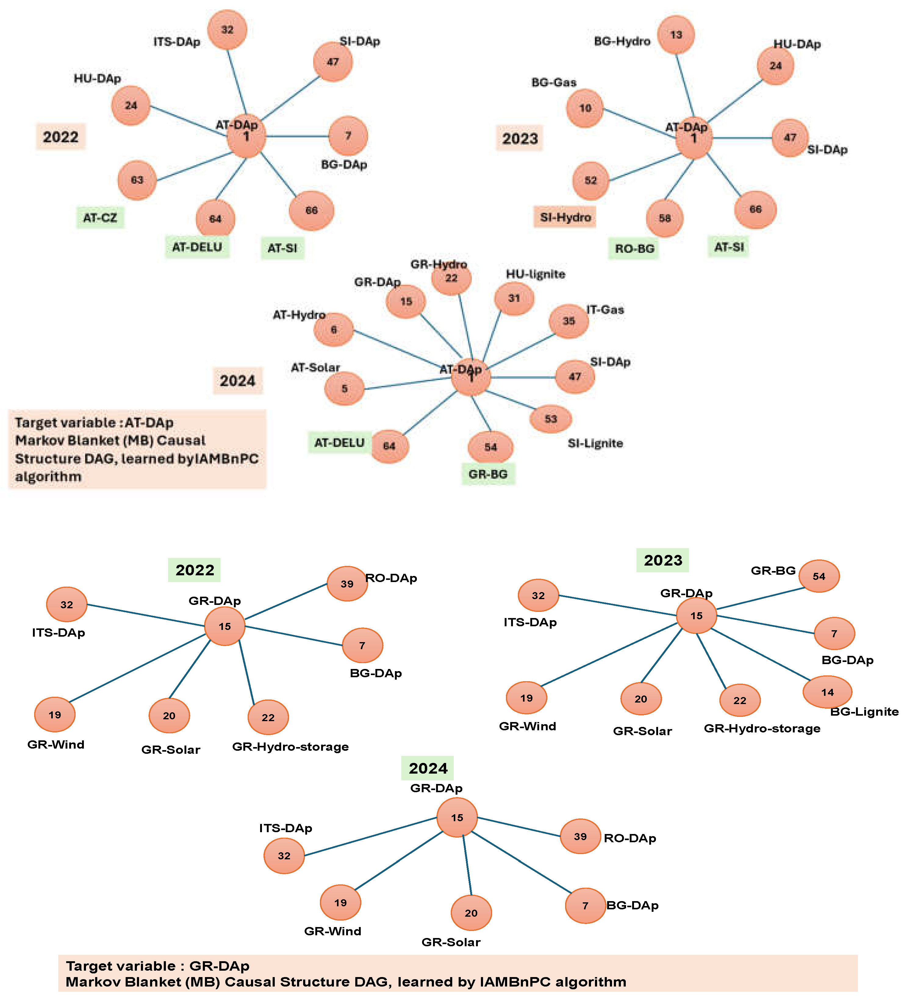
Figure 14.
DAG of the MB causal structure, learned by the IAMBnPC algorithm, for ITS-DA price target variable, for years 2022 to Oct. 2024. DAG is based on Table 14 that contains the nodes (members) of the NB, for each year and each target variable (spot price).
Figure 14.
DAG of the MB causal structure, learned by the IAMBnPC algorithm, for ITS-DA price target variable, for years 2022 to Oct. 2024. DAG is based on Table 14 that contains the nodes (members) of the NB, for each year and each target variable (spot price).
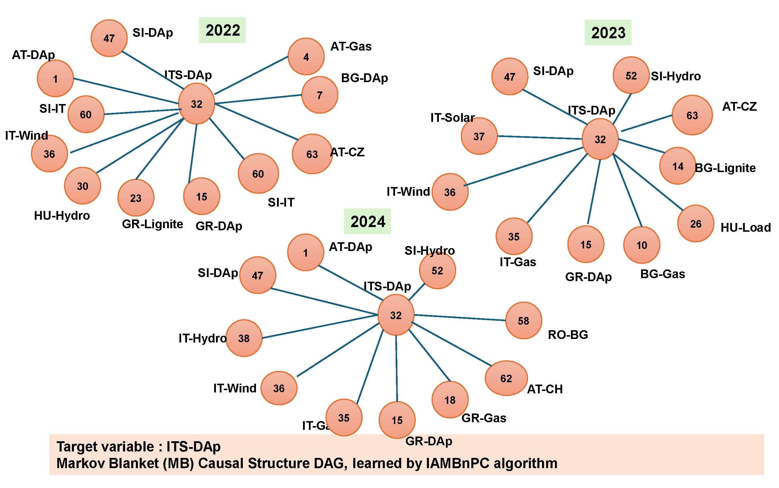
7.2. Local Causal Structure Learning LCSL Results
Having determined the Markov Blanket for each spot price, we proceed to determine the causal relationships within it (i.e. between its members).
We used the CMB algorithm [15], a very suitable method for real-world noisy data, as well as very large data matrices (in our case, the data matrices have 8761 rows and 67 columns, for full year hourly values). Table 15 summarizes the results. The table contains the MB found components, but now with directions, and extends the results including further variables in the DAG, due to the inhered wider ‘lenses’ of the LCS learning model.
From Table 15 we see that in 2022 the parents (direct causes) of Austria’s spot price, AT-DAp, are the Austria’s CBTAs with CZ and DELU (AT-CZ, AT-DELU) i.e. AT-DAp is the child of these two cross border availabilities, which are also members of its MB (see Table 14). Thus, these two CBTAs seem to be the ‘initiators’ of the price volatility disturbances that ‘propagates’ through the entire path from the Core CCR to the SEE CCR. In this year, AT-DAp has the spot prices of HU, ITS and SI, and the AT-SI CBTA as its children. AT-Solar, HU-DAp, SI-DAp and the RO-BG, SI-IT and AT-DELU cross-border transfer availability cause Austria’s price in 2023, which in turn causes the level of the Austria’s Gas generated power (AT-actGAS) and the price of RO, the parents of which in these year, as will be shown in the analysis of RO market, are AT’s spot price and Solar power generation. In 2024, AT-DAp has no direct effect (child) and is affected by a several factors: its parents are Austria’s Solar and Hydro generated power, BG price, Greece’s Hydro, Hungary’s Gas and lignite power production, Italy’s Gas generated power, Slovenia’s spot price and lignite generation, and finally the GR-BG cross-border trading. Figure 15 depicts graphically the results above.
Figure 15.
DAG of the LCSL (local causal structure), learned by the CMB algorithm, for AT-DA price target variable, for years 2022 to Oct. 2024 (Green boxes are used for CBTAs).
Figure 15.
DAG of the LCSL (local causal structure), learned by the CMB algorithm, for AT-DA price target variable, for years 2022 to Oct. 2024 (Green boxes are used for CBTAs).
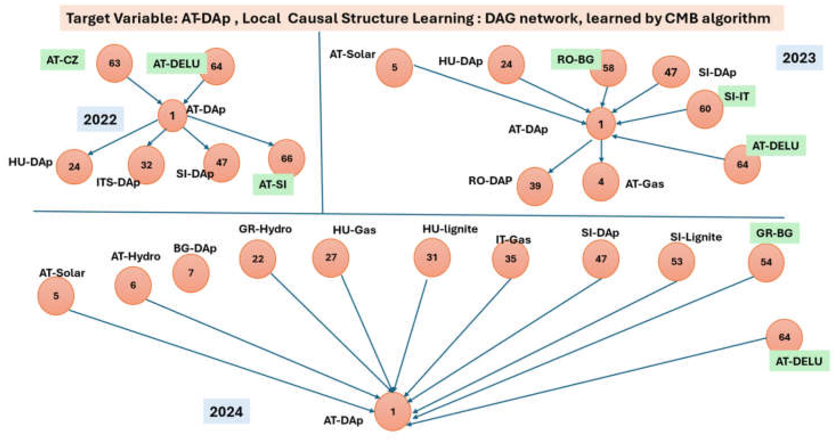
Bulgaria’s spot price (BG-DAp) in 2022 is affected by (its parents are) the spot prices of AT, GR and RO (AT-DAp, GR-DAp, RO-DAp), and the AT-Hydro, GR-wind, IT-Gas, and finally RO- Gas and Lignite. BG-DAp has no direct effects (child) this period. In 2023, AT-Solar, GR-DAp, HU-Lignite, SI-Hydro, CBTAs SI-IT and AT-SI are parents of Bulgaria’s spot price, which in turn has direct effects (children) the HU-wind power generation and Romania’s spot price (RO-DAp). During 2024, HU and RO spot prices are the causes of Bulgaria’s price, which affects (has children) the Greece’s spot price and hydro generation, and Slovenia’s Gas generated power.
In 2022, Greek spot price has as parents the spot prices of Bulgaria’s, Romania’s, Italy’s and Slovenia’s spot prices (BG-DAp, RO-DAp, ITS-DAp, SI-DAp), and Greece’s wind generated power, and affects Greece’s and Romania’s hydro power generation. During 2023, Bulgaria’s price and gas and lignite generated power, Greece’s levels in wind power and hydro storage, and finally Italy’s price and solar generation are the causes of GR-DAp, which in turn has no children (effects). Italy’s, Bulgaria’s and Romania’s spot prices, Greece’s wind and solar power generation, and Romania’s hydro and lignite generations are the causes of Greece’s spot price in 2024, which in turn has no direct effects.
Hungaria’s spot price (HU-DAp), in 2022, has as parents the spots prices AT-DAp, RO-DAp and Greece’s Gas power generation, and Romania’s wind power generation and has direct effect (children) the SI-DAp. Austria’s, Romania’s and Slovenian spot prices, Bulgaria’s, Greece’s and Slovenia’s Hydro power generations, and HU load and Solar generation, are the causes of HU-DAp, in 2023, which in turns has no direct effects. RO-DAp causes the Hungarian spot price in 2024, which has direct effects the BG and SI spot prices, HU gas and solar power generation, the RO wind generation and finally the CBTA BG-GR.
The Italian spot price in 2022, was affected by (caused by) BG’s price and CBTA IT-SI, and has caused AT’s, SI’s, GR’s spot prices, BG’s gas generation, GR’s lignite, HU’s hydro and Italy’s wind power generation, as well as the cross-border transfer availabilities SI-IT, IT-GR and AT-CZ. In 2023, BG’s, GR’s and SI’s spot prices, HU’s and AT’s Solar generations, IT’s gas and wind generations, SI’s hydro generation, and the AT-CZ CBTA were its parent (caused by). AT’s and GR’s spot prices, GR’s gas generation, and IT’s hydro and wind generations were the parents of Italy’s spot price in 2024, which caused the CBTAs RO-BG and AT-CH, and IT’s gas generation.
In 2022, Romania’s spot price was caused by BG’s, GR’s and HU’s spot prices, as well as by RO’s wind generation, and the CBTAs AT-CH, AT-HU, and IT-GR, while ha no directs effects. Its parents in 2023 were the AT’s, BG’s spot prices, and AT’s Solar and IT’s Gas power generations, and has directly affected the Hungarian price. With parents in 2024 the BG’s, GR’s, HU’s and SI’s spot prices, it has directly affected the GR’s and RO’s lignite generations
The parents of Slovenian spot price in 2022, were AT’s price, BG’s Solar and IT’s hydro generations, and has affected the HU’s and IT’s prices as well as the CBTA AT-DELU. In 2023, its parents were the AT’s, HU’s, RO’s prices and the CBTA AT-IT North. In 2024, AT’s, BG’s HU’s spot prices as well as SI’ gas generation were its parents.
7.3. Results of Rolling Price Volatility Correlation and Cluster Analysis for Studying Spillover Effects.
Figure 16 and Figure 17 show the rolling volatility curves of all DA prices, Figure 18 and Figure 19 the rolling volatility of all CBTA, and Figure 20 and Figure 21 the correlation of rolling volatilities and their dendrogram depicting the clustering process, respectively.
In Figure 16 we observe a relative resemblance in the dynamic behavior of spot price volatility of AT, BG, HU, are almost similar. More specifically, the volatility curves trend initially upwards during the third quarter of 2022, and then downwards in the 4th quarter of 2022, although in the case of AT and HU we see a rather oscillating behavior before the end of the 3rd quarter. In the case of ITS and RO prices (Figure 17), the downward volatility is strongly oscillating. The volatilities of all spot prices remain low during the 1st and 2nd quarters of 2023, trending upwards reaching their peak values in the 3rd quarter, trending downwards in the 4th quarter of 2023, remaining at very slow values during the 2nd and 3rd quarters of 2024, and finally trending upwards and reaching peak values during the 3rd quarter of 2024. We can therefore observe clearly in Figure 16 and Figure 17, the decoupling in volatility terms, in the summer 2024: GR, BG, RO and HU have high volatility probably because of the difference in prices between day and night. On the other hand, the volatility of prices in IT and AT is relatively low, while SI’s volatility is somewhere in the middle. Looking at the other time periods of our analysis, from 2022- Oct.2024, we observe identical volatility shapes.
In Figure 18 and Figure 19, we show the curves of the rolling volatility of cross-border trading, CBTA, between the markets shown in the figures. During 2022, the volatility of CBTA between Austria and Switzerland (AT-CH) exhibits strong oscillations, with peaks in the middle of the 2nd and 3rd quarters, as well as at the ends of the 1st and 4th quarters. In 2023, the volatility is constantly at a high level in the 1st quarter, shows a V shape in the second, and drops in the third, while increasing during the 4th quarter, taking its peak value at the end of 1st quarter of 2024.
A strong increase in volatility is observed during 2nd and 3rd quarters of 2024, reaching its lowest value near the end of August 2024, followed by an abrupt upward trend at the end of 3rd quarter of 2024. The rolling volatility of the CBTA between AT and CZ exhibits an strong decrease at the end of 2022 2nd quarter, remaining constantly at a very low value up to the 2023 1st quarter, followed by a lasting increase up to the end of 3rd quarter of 2023, after which a dropping and an increasing behavior is observed in the 4th quarter, then remaining constant for the rest of the periods. The rolling volatility CBTA between Austria and Germany (AT-DE), shows an abrupt decrease and then increase in 2022 Q1, remains constant during 2022 Q2 and Q3, drops and increase fast in 2022 Q4, and remains constant at a high value for the rest of 2023-24 period. The rolling volatility of CBTA between Austria and North Italy (AT-ITN), exhibits a constant dropping in the first three quarters of 2022, increases to a peak value in the middle of 2022 Q4, followed by a fast dropping and then is trending upward with oscillations, for the rest of the periods. The rolling volatility of CBTA between Austria and Hungary (AT-HU), is low in the first three quarters of 2022, followed by a upward trending and reaching a peak value in 2022 Q4, and finally exhibits an upward oscillating trend up to the 1st quarter of 2024,
7.3.1. Correlation of Rolling Volatility Curves and Their Clustering Process
The interaction of all rolling volatility curves, described previously, is shown in Figure 20, where the correlation of rolling volatility curves of all DA prices and all CBTAs (using a window of 720 hours-1 month), is shown. Using the information above, and in combination with the results of CBTA’s rolling volatility correlation, Figure 20, we can ‘capture’ the dynamics of the volatility spillover, trying to detect significant decoupling in volatility patterns that may indicate cross-border disruptions that cause the increase in the spot prices in this region. In Figure 20 we observe a relative heterogeneity in the context of correlation of rolling volatility, across markets: the Italian and Austrian markets are shown to have lower correlation of price volatility (see ‘orange’ upper-left cells in Figure 20). For example, volatility correlation of ITS with HU (0.69), SL (0.75), AT (0.80), RO (0.74) and BG (0.74), GR(0.74) markets, indicating that the correlations (a linear measure) of price volatilities are lower between geographically distant and unconnected (directly) markets. However, we observe that RO and BG markets, although distant and not directly connected with the IT market, exhibit larger correlations with ITS than with HU market, and comparable with SI market. This ‘strange’ result is justified by the ‘weaknesses of this linear measure, as well as from the results of the MB and LCS learning, Section 7.1 and 7.2. From the MB and LCS analysis (see Table 14 and Table 15), the GR-DA price (15) has parents the BG-DA price (7), whose parent is the RO-DA price (39), as well as the ITS-DA price (32). The moderate correlations of price volatility of RO-DA and BG-DA prices with the Italian price is due to this indirect connection, reflecting their nonlinear correlation, ‘captured’ via MB analysis. The correlations of price volatility between the directly connected markets are the highest, as shown in Figure 20 (yellow and orange cells, in the upper-left portion of the figure).
Thus, markets AT, HU, RO, BG seem to be the best candidates for volatility transmitters, and since AT is the first market in the entire interconnection path, seems to be the most critical market, most likely the initiator of the propagation of the price surges in SEE region. This is shown below, by examining the volatility spillover across markets via a dendrogram (see Figure 21) of the correlation of volatility values.
The highest correlations of price volatility of the Greek market are with the RO and BG (~0.948 and ~0.95 respectively), and smaller but statistically significant ones with all other markets. The results of the rolling volatility shown in the figures are consistent with the results of the MB and LCS learning which effectively contribute to capturing both linear and nonlinear spillover mechanisms of the price volatility of all markets directly and indirectly connected.
We then examine how the spot price volatility correlation of the two groups of countries, the group DE/AT/HU and the group RO/BG/GR, are compared. For the first group the correlations are corr(ATp-Hup) = 0.65, corr(ATp-BGp) = 0.72, corr(ATp-GRp) = 0.69 and ATp-ROp) = 0.70, so the mean correlation of the group is 0.69. Similarly, corr(ROp-GRp) =0.77, corr(ROp-BGp) =0.98, corr(GRp-BGp) =0.957, giving a mean volatility of 0.90. Thus, the rolling spot volatility within SEE CCR group (BG, GR) and RO increases, driven by shared scarcity shock. We also observe a drop in the volatility correlation between the two groups, from 0.90 to 0.69, indicating that the SEE CCR countries become their own self-contained volatility bubble, while core markets experience minimal impact (at least temporarily) (all above correlations are statistically significant).
We examine and compare now the volatility correlations between spot prices and CBTA, in each of the two groups. We observe statistically significant negative volatility correlations in pairs of AT-CH cross-border trading and the spot prices: corr(ATp-(AT-CH)) = -0.353, corr(BGp-(AT-CH))=-0,56, corr(GRp-(AT-CH)) = -0.48, corr(Hup-(AT-CH)) = -0.64, corr(ROp-(AT-CH)) = -0.59, corr(SIp-(AT-CH) =-0.65. Similar negative volatility correlations between Austrias’ CBTAs with other central Europe (core) countries and SEE spot prices, are observed. Thus, when Austria decreases its CBTA with countries that are interconnected with SEE countries, causes their spot prices to increase substantially.
How are the above results of the rolling volatility spillover related to the Target’s model expected ‘behavior’? We know that Target Model + Flow-Based Allocation → Market Distortion. The Target Model’s flow-based market coupling (FBMC) assumes "physical feasibility optimization” but in practice, its algorithms allocate cross-border capacities not just based on price signals but also on pre-set constraints and priorities. Since, as we know, flows were redirected to Switzerland (CH) and Ukraine, then SEE markets became de facto semi-isolated, losing competitive imports from cheaper markets (DE/AT/HU). As a result, we can conclude that price and volatility in SEE spike due to a) supply scarcity, b) loss of arbitrage smoothing and c) increased reliance on local (often more expensive) generation. This finding however, raises a new relative question: Is there strategic behavior/ “price game”? This is subtle. While it's unlikely that Germany/Austria/Hungary are explicitly “playing a price game”, the structure of FBMC allows passive gain from structural decoupling:
- When interconnection is “algorithmically blocked”, SEE CCR market prices surge, but DE/AT/HU can export at higher prices via different paths (or even import cheap and export expensive).
- If cross-zonal capacities are not allocated efficiently, this can create rent-seeking arbitrage opportunities, especially for dominant players (e.g., traders, utilities) in the core.
Therefore, our answer could be yes! However, this may not be malicious intent, but the algorithmic structure enables economic rents to concentrate in the core zone, leaving SEE markets overexposed.
7.3.2. The Dendrogram of the Clustering Process
Figure 21 shows the twenty (20) hierarchically formed clusters in a dendrogram, shown also in Table 16. We describe shortly the process of clustering of the correlations of spot prices and CBTAs volatilities, to shed further light on the way they interact: RO-DAp and BG-DAp cluster first (cluster 1), by the first U-shaped lines connecting RO and BG in the hierarchical tree. The height of U-shaped lines corresponds to the lower distance (~0.30) between the two data points, i.e. to the highest correlation between their rolling price volatilities. The next cluster (cluster 2) is that between HU spot price and the previously formed cluster of RO and BG prices, with a distance slightly larger than before, i.e. HU price has a lower correlation between its volatility, or the spillover of volatility between HU and the two markets of BG and RO is lower than the spillover of volatility between BG and RO.
Figure 21.
Dendrogram showing the clusters of the rolling volatility of DA prices and CBTA. Numbers show the hierarchical position of the clusters, characterized as leaders, early and late followers. The highest strength of volatility spillover is shown by the leader clusters.
Figure 21.
Dendrogram showing the clusters of the rolling volatility of DA prices and CBTA. Numbers show the hierarchical position of the clusters, characterized as leaders, early and late followers. The highest strength of volatility spillover is shown by the leader clusters.
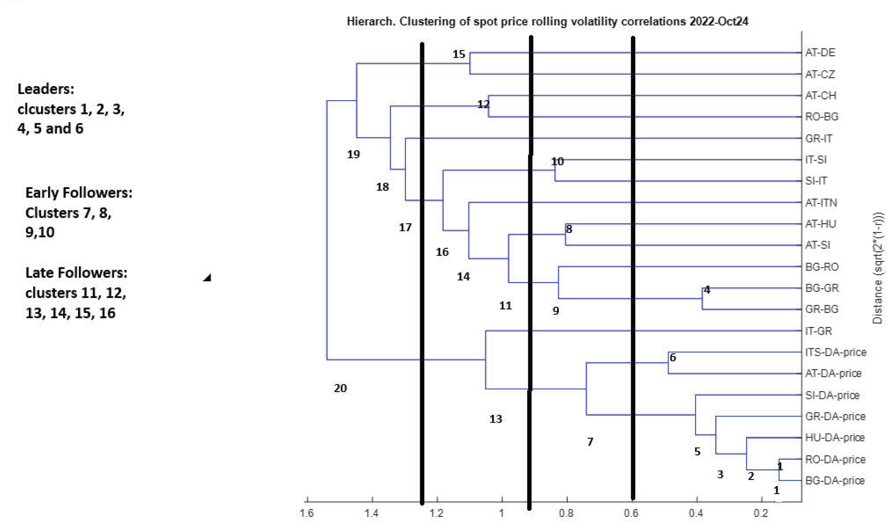
The next cluster (cluster 3) is formed between the previously clusters of (RO-BG) and HU-(RO-BG) with GR price, where the height of U is considerably larger (~0.35), indicating that the correlation of price volatilities between the markets of the two previous clusters and GR is lower, i.e. the strength of the volatility spillover between the GR and (RO-BG) and HU-(RO-BG). The process of clustering continues similarly, so the next cluster (4) is between the CBTA between Greece and Bulgaria, followed next by the cluster (5) between the spot prices of SI and the spot prices of cluster 3. Then cluster 6 is between ITS (Italy South) and Austria (AT) spot prices. Thus, interestingly, the spillover of volatility between AT and ITS prices is weaker than the spillover between BG and GR CBTAs, a very interesting finding. Table 16 shows the hierarchical steps from cluster 1 to cluster 14 of the clustering process. The cluster 8 made by CBTAs of AT-HU and AT-SI) with cluster 9 (BG-RO and (BG-GR and GR-BG) is pivotal, since it emphasizes strongly how the CBTAs of AT, HU, SI, BG, RO, and GR markets interact with, i.e. how the volatility of Austria’s CBTA spills over to the markets of BG and GR. The clustering of the AT-CH and RO-BG CBTAs (cluster 12) also enhances the strong interaction between the AT and CH markets with the two SEE markets of BG and RO! Similarly, CBTAs between Austria’s and Germany’s (AT-DE) and Austria’s and Czechoslovakia’s (AT-CZ) electricity markets (cluster 15), also indicates that the Austrian market is a pivotal market, more importantly it is a ‘transmitter’ of price and cross-border activity volatility, between markets that are located ‘up-stream’ and ‘down-stream’ in its connection path with SEE markets that receive the price and CBTA volatility disturbances that cause their price surge. Table 16 shows the hierarchy of the clustering process. Clusters 1, 2, 3,5,6 and 7 refer to pairs of several DA prices while the rest to the pairs of CBTAs. From all the above and looking carefully at Figure 21 and table 16, we will try to make further distinction between the markets, based on the hierarchy of their clustering process. More specifically, we identify markets as leaders, early and late followers, according to the priority of clustering patterns. Also, we identify Bridge markets, the ones that connect the Central Volatility Zones markets with the South Volatility Zones markets. Therefore, based on Figure 21 and Table 16, the leaders are the clusters 1, 2, 3, 4, 5, and 6, formed mainly by the spot prices and the CBTAs BG-GR and GR-BG, while early followers are the clusters 7, 8, 9, 10, formed only by cross-border trading availabilities (CBTAs), and finally late followers, formed by clusters 11, 12, 13, 14, 15 and 16, also by clusters formed only by CBTAs. Clusters 17-20 (not shown) indicate clusters of markets interactions with negligible spillover effects. It is obvious that the markets involved in the early followers volatility patterns can also be the bridge markets.
From the dendrogram and specifically the leader clusters we observe the intensive volatility spillover between BG and RO spot prices, as well as the intensive volatility spillover between the spot prices of HU and BG, HU and RO, and between GR, BG and RO. The volatility spillover of cross-border transfer availability between BG and GR is also intensive. Intensive is also the volatility spillover of AT and ITS prices (cluster 6), which affects all the previous spot prices. The conclusion here is that the volatility of spot prices of three Core CCR markets (HU, AT and RO), is diffused towards and affects severely both the spot prices as well as the CBTAs of BG and GR. The spillover of volatility is lower between the spot prices or CBTAs of the markets belonging to early clusters, e.g. the CBTAs IT-SI, AT-HU and AT-SI, also the CBTA BG-RO with BG and GR, which also is diffused and affects the spot prices of the SEE CCR markets of Greece and Bulgaria. Therefore, the clustering process shown in the dendrogram creates a structure of interactions between the pairs of quantities in the clusters (mainly leaders & early followers), a ‘suitable background’ in which if crucial events occur can ‘fire’ the formation of price spikes and surges, that can propagate towards the RO, BG and GR markets. Thus, if a disturbance in prices or CBTAs take place in the ‘upstream’ (say AT, HU) of this ‘background’, the induced volatilities diffuse to ‘downstream’ markets of BG and GR.
Under the light of the results, we examine the period 2023–2024, and specifically how the Electricity flows (indicated by the dendrogram above) between Austria (AT), Czechoslovakia (CZ), Switzerland (CH) and Germany (DE), in a cascading mode, have affected the dynamics of flows to Hungary and then to SEE CCR countries Bulgaria, Greece and Romania (a Core CCR member).
Table 16.
The hierarchy of the clustering process.
|
Cluster hierarchy |
Market fundamentals |
Cluster hierarchy |
Market fundamentals |
| 1st cluster | ROp-BGp | 9th cluster | BG-RO cbta with cluster 4 |
| 2nd cluster | HUp with cluster 1 | 10th cluster | IT-SI cbta with SI-IT |
| 3rd cluster | GRp with cluster 2 | 11th cluster | cluster 8 with 9 |
| 4th cluster | BG-GR cbta with GR-BG cbta | 12th cluster | RO-BG with GR-IT |
| 5th cluster | SIp with cluster 3 | 13th cluster | IT-GR cbta with cluster 7 |
| 6th cluster | ITSp with ATp | 14th cluster | AT-ITNorth cbta with cluster 11 |
| 7th cluster | cluster 6 with 5 | 15th cluster | AT-DE with AT-CZ cbta |
| 8th cluster | AT-HU cbta with AT-SI cbta | 16th cluster | cluster 10 with 14 |
An important question then is raised, regarding possible supply disruptions not naturally occurred but ‘artificially’, because of an algorithmic idiosyncrasy of the relevant mechanism. More specifically, by "artificially disrupted" we mean disrupted not by real physical constraints (like lines overloaded) but algorithmically by the market coupling rules incorporated in the Target Model, especially flow-based market coupling (FBMC)), that can even redirect flows toward ‘wrong’ countries. The complexity of the interactions described by the dendrogram above, that have created a ‘suitable background’ awaiting for crucial events to happen to generate price spikes and surges, can be revealed by summarizing the situation as follows. The background is that Germany, Austria, Switzerland, and Czechia are tightly interconnected and were historically considered a "copperplate" (no internal congestion). Switzerland is not in the EU Target Model (due to political reasons), but physically it’s important. Since October 1, 2018, Germany and Austria are split into separate bidding zones because of loop flows that affected Eastern Europe, especially Hungary. As already mentioned, Flow-Based Market Coupling (FBMC) is now active in the Core region (which includes AT, CZ, DE, HU, RO, etc.) since June 8, 2022. We now shortly review what happened in 2023–2024. Due to excessive renewable generation (i.e. surpluses especially in Germany) and market prices differences (especially after the Ukraine war energy crisis), electricity was flowing massively from North and Central Europe toward the South-East. Hungary (HU) became a critical transit and bottleneck country. Constraints on cross-border flows between DE–CZ, DE–AT, and AT–HU, have become dominant in the calculation. Some flows were redirected4 or "allocated differently": flows that "were supposed or wanted" to go to HU, RO, BG were sometimes "virtually" limited because of congestion elsewhere (even if the physical lines HU–RO were not full). Ukraine’s interconnection with EU (via ENTSO-E synchronization) after February 2022 allowed for commercial exchanges — mainly export from EU to Ukraine. So, the natural question that now oppressively is raised is: was this redirection an artificial one? In a sense, we answer yes, based on the findings above and the following scenario-argument: under the flow-based allocation, if an export from Germany to Romania/Hungary uses critical branches (lines) that are already congested (say in CZ or AT), then the market coupling limits how much can be sent, even if locally the HU–RO line is not congested. Meanwhile, exports to Ukraine (through Slovakia or Hungary) could still happen because they use different critical branches, or because their allocated flow factor is lower. This means that even if physically we could have sent more toward Romania, the algorithm limited it — not because of real-time physical overload, but because of calculated capacity margins. Figure 22 shows the physical connections: DE (Germany), AT (Austria), CZ (Czechia), CH (Switzerland), HU (Hungary), RO (Romania), BG (Bulgaria), GR (Greece), UA (Ukraine), as well as how flows were meant to go toward RO and SEE CCR (HU → RO → BG → GR). Most importantly, it depicts also how algorithmic flow-based rules limited flows toward SEE but allowed flows to Ukraine. Specifically, it shows that normally electricity should flow DE → CZ → SK → HU → RO → BG → GR (the right path), but the TM’s algorithm for flow-based market coupling (FBMC) ‘realized’ a congestion in CZ and AT (mainly because Germany’s renewable surpluses heavily loaded internal grids), resulting therefore in limited electricity transfers toward HU and further into RO/BG, regardless the fact that the HU→RO line was physically free. However, export HU→UA (Ukraine) was allowed because it had a lower impact on congested lines (different PTDF, see footnote 4). Therefore, RO and SEE CRR markets (BG, GR) sometimes due to limited-reduced electricity imports exhibited higher prices. Table 17 provides a short visual summary of the results of Figure 22.
7.3.3. The Behavior of the Target Model in the Issue of SEE Markets’ Price Surge
Based on the results depicted in Figure 22 and Table 17, we ask whether the European Target model has failed in our case, in the sense that it has not prevented the prices surge in SEE countries in the period 2023-2024. Having accepted in the previous section that the flow redirection was ‘artificial’, we further dig into it carefully, since the answer seems to be nuanced, not a simple ‘yes’ or ‘no’. First, a summary of what the European Target Model (ETM) was supposed to do is shown in Table 18. TM’s Flow-Based Market Coupling (FBMC) mechanism plays a crucial role in the performance of the model when applied in practice, since it models the real physics of the grid better than simple border-based allocations. An evaluation of the TM’s performance in dealing with the wholesale price discrepancies and surges in SEE CCR markets is given in the comments of Table 18. Therefore, our answer to the question is partly yes. Table 18 shows a detailed evaluation of the TM’s performance, in the case of SEE prices surge.
As a conclusion, although TM’s FBMC algorithm obeyed its design rules, price convergence and "social welfare" goals were not achieved for SEE CCR markets, a finding of strategic consequences, as the need for Europe to split large bidding zones further (e.g., Germany into north/south zones, now a real fact) (ENTSO-e, 2025, [52]), as many experts have systematically argued. Another strategic consequence is the need to invest massively in North–South transmission corridors (e.g., from Poland to Romania, from Austria to Hungary and further ‘downstream’ to South). Also, considering all the TM’s ‘malfunctions’ generated due to exports to Ukraine, mentioned previously, it is urgent for Europe review priority treatment of Ukraine export vs internal EU flows in critical times, on a higher strategic level, considering also the need of adjusting flow-based rules to better protect the markets in vulnerable regions like SEE CCRs markets. Conclusion: the European Target Model worked mechanically, but failed strategically for SEE countries in 2023–2024 — it did not deliver price convergence or fair market integration for them under stress.
8. Discussion - Conclusions and Policy Recommendations
The findings in Section 7 have shown that by applying a combination of ML methods (Markov Blanket, MB, and Local Causal Structure- LCS- learning approaches) with a mainstream approach, the analysis of volatility spillover effects between pairs of markets analyzed in this paper, has been proved to be a powerful tool for causal feature descovery, helping to reveal the strongest factors influencing (causing) the dynamic evolution of the surges of DA electricity prices occurred in the SSE CCR countries, in the period of 2023-2024.
By focusing on causally relevant features, the tool improves model interpretability and predictive performance while avoiding overfitting caused by irrelevant or redundant variables. We have shown how Markovian Blanket, a causal feature selection and discovery approach, has revealed the strongest factors in explaining the price surges in SEE electricity markets. We have also shown why this approach is better than a typical regression approach, in our case. Using the Markov Blanket for causal feature selection and discovery to explain price surges in SEE electricity markets has proved to provide us with a robust framework for identifying the strongest explanatory factors, (out of a ‘large’ number of possible market parameters), focusing on causal relationships rather than mere associations. We believe that via these causal interactions we finally managed to shed some light on the ‘real’ factors that shape the DA electricity price surges in the Southeast European countries.
To further enhance our results, we computed the rolling volatility curves of all crucial variables included in the MB sets, for each market, and their correlations to detect volatility spillovers, across the entire path of the spot prices and CBTAs, from north to south markets, to detect how ‘volatility disturbances have propagated. The combination of MB-LCS learning and Volatility Spillover analysis revealed the ‘partial failure’ of the European Target Model’s capacity to protect the price surge in SEE markets, i.e. we have found that TM facilitates cross-border price crisis diffusion.
Our findings have successfully explained how the transformation, via the target model, of a local problem of supply-demand imbalance into an electricity price problem (due to energy exchange market inflation) and then the spillover-diffusion of this problem to the entire path of the interconnected countries (DE-LU →AT→HU→RO→BG→GR), has challenged the effectiveness and reliability of the target model, as a mechanism designed to ‘homogenize’ prices and more importantly in mitigating price surges in a network of coupled electricity markets, thus its contribution to the energy transition target is seriously criticized.
8.1. Policy Issues and Future Directions
As we have already pointed out in Section 4, several factors seem to have exacerbated FBMC's challenges in the case of SEE CCR’s countries: a) the limited interconnectivity, since these countries often rely on the Net Transfer Capacity (NTC) mechanism, contrasting with FBMC's application in Core CCR’s countries. Thus, this discrepancy seems to hinder their seamless integration into the European ‘core body’ power system, b) infrastructure constraints, as the delays in returning key power plants, maintenance on critical interconnectors, such as the BG>RO line, further strained the system, and finally c) external (weather) pressures, as climate events, like heatwaves, have increased electricity demand, while geopolitical tensions, notably Ukraine's shift from exporter to importer, added pressure on neighboring grids.
We conclude that while FBMC is designed to enhance market efficiency and integration, its current implementation has, in certain scenarios, failed to protect SEE markets from spot price surges and discrepancies compared to Central European markets. The July 2024 events exemplify how algorithmic decisions, without adequate consideration of regional specificities and infrastructure limitations, can lead to significant market distortions. Addressing these challenges requires a reevaluation of FBMC's application in SEE, improved infrastructure, and enhanced coordination among regional stakeholders.
Based on the results of the study, and specifically on the ‘response’ of the Target model (TM) to the systematic discrepancies of spot prices between Core CCR and SEE CCR markets, we have already addressed the challenges imposed on TM due to its ‘partial failure’ in dealing with this issue. Therefore, to strengthen Target Model's capacity in successfully handling a future prices problem in Southeast Europe, we propose several measures that seem to be necessary. First, the need for accelerating market coupling, i.e. enhance cross-border market integration and expand interconnection capacity, as well as investing in regional grid infrastructure to reduce bottlenecks, are immediate actions to be taken. Secondly, the diversification of energy sources, via prioritizing the deployment of renewables, particularly wind and solar, to reduce reliance on volatile fossil fuels, and supporting energy storage solutions and demand-side management, are also urgent actions. Regulatory and Institutional Reforms are also needed, to strengthen market competition and reduce the dominance of state-owned utilities in the region under analysis, as well as a need to harmonize regulations to align with EU standards and foster investor confidence. The Target model must adopt crisis-preparedness mechanisms, i.e. developing tools to address price volatility, such as capacity mechanisms, strategic reserves, and demand response programs. The model must also facilitate coordination of regional efforts to manage energy security and supply risks. As a conclusion, the Target Model has not failed outright, but its shortcomings in Southeast Europe highlight the need for targeted reforms and investments. Addressing structural weaknesses and accelerating market integration are critical to ensuring that the region can fully benefit from the model while mitigating the impacts of future energy crises.
8.2. Need for an EU-Wide Systemic Approach in Decision Making
It is profound from all above that the EU needs stronger governance – a system that allows it more input into decisions made by individual countries that could have regional effects, such as planned outages. Therefore, a strong request is for more EU regulatory oversight, an EU-wide regulator for electricity that can have a systemic-holistic as well as ‘concurrent’ view of all interconnected and interacted markets. Another crucial issue, revealed by this price surges is that the decision for exporting to Ukraine has created a strong impact, that however is felt only by some countries without sufficient electricity transfers within the EU. Thus, it seems that there is a need for re-designing electricity market for options for Greece to ‘claw back windfall (unexpected) profits from generators and protect consumers during this shock’, as the Greek Prime Minister stated. Thus, Greece, Bulgaria and Romania have expressed jointly the need their interconnection projects to be funded from profits from the wholesale electricity markets. Greece already charges a windfall (unexpected) tax on energy companies and directs the proceeds in the form of subsidies to vulnerable consumers. In the current framework the EU allows market interventions but with a substantial lag, i.e. after a prolonged period of high prices. The three badly affected from the prices surges countries, Greece, Romania and Bulgaria, have expressed their request for a mechanism that will enable them to react faster to the price spikes. The price disparities also have revealed the need for the EU to enhance electricity interconnectors, so in case these disparities between countries reach extreme levels make the related interconnection projects strongly justifiable due to enhanced cost-benefit considerations. Thus, the three Balkan countries have requested that part of their revenues from electricity markets be invested in the development of the grids enhancing and their cross-border transfer availability (CBTA).
8.3. Potential limitations, Challenges & How to Overcome Them
We list at this point some possible limitations in our work as well as the actions we have taken to strengthen further the reliability of our findings: a) Data Quality: Causal discovery needs high-quality, time-synchronized data. In this study we used reliable and tested data provided by the European organization ENTSO-E, as well as regulatory reports for Greece and other SEE markets, b) Latent Confounders: we could extend the current study by applying Bayesian methods to account for unobserved effects like political risks, a work left for future consideration, c) Computational Complexity: the algorithms used in this work are very efficient in handling very large datasets, even larger than those used in our work.
Supplementary Materials
The following supporting information can be downloaded at the website of this paper posted on Preprints.org.
| 1 | Biding zone: the largest geographical area where energy exchange can take place between players without capacity calculation. |
| 2 | Full:<1 Euro/MWh, Moderate: 1-10 Euro/MWh, Low: >10 Euro/MWh) |
| 3 | Two possible methods the EU rules allow for TSOs to calculate the capacity made available for trade between EU bidding zones in a coordinated manner: the coordinated net transfer capacity (CNTC) approach and the flow-based (FB) approach. The CNTC approach, can be applied in regions where cross-zonal exchanges are less interdependent, therefore no significant added value is expected to be gained from adopting the FB approach. The FB approach is defined as the default in areas of the transmission grid where the exchanges across bidding zone borders are highly interdependent, and models only a subset of network constraints, the so-called critical network elements with contingency (CNECs) (a line or transformer either within a bidding zone or between bidding zones). An optimized allocation of cross-zonal capacities at the level of the capacity calculation region is therefore allowed, by the price coupling mechanism that can allocate the capacity made available on each CNEC to the electricity exchanges that generate the largest ‘added social value’. |
| 4 | Commercial flows are redirected (e.g. to Ukraine) because of different impact factors, PTDFs (Power Transfer Distribution Factors) determine how much a MW transfer from A to B uses each line. RAM (Remaining Available Margin) is the headroom left on a line. If a transfer Germany → Romania "uses" too much of a congested line in Austria or Czechia, it's limited. Export Germany → Ukraine (via Slovakia) might "use" less congested lines (or different ones) → so it's allowed. The core flow-based domain thus shapes what trades can happen. |
References
- PMKM, 2024 (Prime Minister Kyriakos Mitsotakis letter to EC, 2024). (https://www.primeminister.gr/en/2024/09/13/34887). Downloaded 23 Dec. 2024.
- ACER, 2024. Transmission capacities for cross-zonal trade of electricity and congestion management in the EU, 2024 Market Monitoring Report, 3 July 2024.
- Draghi, M. (2024). The future of European competitiveness: A competitiveness strategy for Europe. European Commission. https://commission.europa.eu/document/download/97e481fd-2dc3-412d-be4c-f152a8232961_en.
- Pellet, J.P.; Elisseeff, A. Using Markov Blankets for Causal Structure Learning (2008). Journal of Machine Learning Research 2008, 9, 1295–1342. [Google Scholar]
- Aliferis, C.F.; Statnikov, A.; Tsamardinos, I.; Mani, S.; Koutsoukos, X.D. . 2010. Local causal and Markov blanket induction for causal discovery and feature selection for classification part I: Algorithms and empirical evaluation. Journal of Machine Learning Research 2010, 11, 171–234. [Google Scholar]
- Yu, K.; Liu, L.; Li, J. A unified view of causal and non-causal feature selection. ACM Transactions on Knowledge Discovery from Data 2021, 15, 63. [Google Scholar] [CrossRef]
- Hong, Y.; Hao, Z.; Mai, G.; Huang, H. Causal Feature Selection Method Based on Extended Markov Blanket. International Journal of Wireless and Mobile Computing (IJWMC) 2018, 15. [Google Scholar] [CrossRef]
- Băncioiu, C.; Brad, R. Accelerating Causal Inference and Feature Selection Methods. (2021). Entropy 2021, 23, 1501. [Google Scholar] [CrossRef]
- Fu, S.; Desmarais, M.C. Markov Blanket Based Feature Selection: A Review of Past Decade. Proceedings of the World Congress on Engineering 2010 Vol I WCE 2010, June 30 - July 2, 2010, London, U.K.
- Bellizio, F.; Cremer, J.L.; Sun, M.; Strbac, G. A causality-based feature selection approach for data-driven dynamic security assessment. Electric power systems research 2021, 201, 107537. [Google Scholar] [CrossRef]
- Maisonnave, M.; Delbianco, F.; Tohme, F.; Millios, E.; Maguitman, A. Learning causality structures from electricity demand data. Energy Systems 2024. [Google Scholar] [CrossRef]
- Prahara, J.; Hariadi, T.K. Improved Feature Selection Algorithm of Electricity Price Forecasting using SVM. Published in2022 2nd International Conference on Electronic and Electrical Engineering and Intelligent System (ICE3IS). [CrossRef]
- Mitridati, L.; Pinson, P. (2017). A Bayesian Inference Approach to Unveil Supply Curves in Electricity Markets. IEEE Transactions on Power Systems. [CrossRef]
- Maticka, M.; Mahmoud, T. (2016). Bayesian Belief Networks: Redefining wholesale electricity price modelling in high penetration non-firm renewable generation power systems. [CrossRef]
- Nickelsen, D.; Muller, G. Bayesian Hierarchical Probabilistic Forecasting of Intraday Electricity Prices. arXiv:2403.05441v1 [stat.AP] 8 Mar 2024.
- Zholdasbayeva, M.; Zarikas, V. and Poulopoulos, S. Bayesian Networks based Policy Making in the Renewable Energy Sector. In Proceedings of the 12th International Conference on Agents and Artificial Intelligence (ICAART 2020) - Volume 2, pages 453-462 ISBN: 978-989-758-395-7; ISSN: 2184-433X. [CrossRef]
- Borunda, M.; Ballestros, A.R.; Jaramillo Ibarguegoytia, P. (2016). Bayesian networks in renewable energy systems: A bibliographical survey. Article in Renewable and Sustainable Energy Reviews. September 2016. [CrossRef]
- Guo Ying, (.B.).; Ni Yang Wang Yuan Zhao Jing Liu Liwei Research on Power Marketing Decision-Making Algorithm Based on Bayesian Network In, S.H.B.D.M. Zailani et al. (Eds.): ICMSEM 2023, 259, pp. 1245–1253, 2024. [CrossRef]
- Ling, Z.; Yu, K.; Wang, H.; Li, L.; Wu, X. 2020. Using feature selection for local causal structure learning. IEEE Trans. Emerg. Topics Comput. Intell. [CrossRef]
- Pearl, J. 2014. Probabilistic Reasoning in Intelligent Systems: Networks of Plausible Inference. Morgan Kaufmann.
- Spirtes, P.; Clark; Glymour, N.; Scheines, R. 2000. Causation, Prediction, and Search. Vol. 81. MIT Press.
- Bell, D.; Wang, H. A formalism for relevance and its application in feature subset selection. Machine Learning 2000, 41, 175–195. [Google Scholar] [CrossRef]
- Brown, G.; Pocock, A.; Zhao, M.-J.; Lujan, M. Conditional likelihood maximization: A unifying framework for information theoretic feature selection. Journal of Machine Learning Research 2012, 13, 27–66. [Google Scholar]
- Vergara, J.; Estevez, P.A. A review of feature selection methods based on mutual information. Neural Computing and Applications 2014, 24, 175–186. [Google Scholar] [CrossRef]
- Yu, K.; Ling, Z.; Liu, L.; Wang, H.; Li, J. Feature Selection for Efficient Local-to-Global Bayesian Network Structure Learning. ACM Transactions on Intelligent Systems and Technology.arXiv:2112.10369v1 (2021). [CrossRef]
- Fukunaga, K. 2013. Introduction to Statistical Pattern Recognition. Academic Press.
- Fano, R.M. 1961. Transmission of Information: A Statistical Theory of Communications. MIT Press.
- Hellman, M.E.; Raviv, J. Probability of error, equivocation and the chernoff bound. IEEE Transactions on Information Theory 1970, 16, 368–372. [Google Scholar] [CrossRef]
- Tebbe, D.; Dwyer, S. Uncertainty and the probability of error (Corresp.). IEEE Transactions on Information Theory 1968, 14, 516–518. [Google Scholar] [CrossRef]
- Shannon, C.E. A mathematical theory of communication. ACM SIGMOBILE Mobile Computing and Communications Review 2001, 5, 3–55. [Google Scholar] [CrossRef]
- Kohavi, R.; John, G.H. Wrappers for feature subset selection. Artificial Intelligence 1997, 97, 273–324. [Google Scholar] [CrossRef]
- Tsamardinos, I.; Aliferis, C.F. 2003. Towards principled feature selection: Relevancy, filters and wrappers. In Proceedings of the 9th International Workshop on Artificial Intelligence and Statistics. Morgan Kaufmann Publishers.
- Koller, D.; Sahami, M. 1995. Toward optimal feature selection. In Proceedings of the 13th International Conference on International Conference on Machine Learning. 284–292.
- Guyon, I. Constantin Aliferis Andre Elisseeff 2007 Causal feature selection Computational Methods of Feature Selection, H. Liu and H. Motoda (Eds.). CRC Press.
- Margaritis, D. and Sebastian Thrun. 2000. Bayesian network induction via local neighborhoods. In Proceedings of the Advances in Neural Information Processing Systems. 505–511.
- Tsamardinos, I.; Constantin, F. Aliferis, Alexander R. Statnikov, and Er Statnikov. 2003b. Algorithms for large scale Markov blanket discovery. In Proceedings of the FLAIRS Conference. Vol. 2. 376–380.
- Yaramakala, S. and Dimitris Margaritis. 2005. Speculative Markov blanket discovery for optimal feature selection. In Proceedings of the IEEE International Conference on Data Mining (ICDM’05). IEEE, 4–9.
- Cevic, S.; Zhao, Y. Shocked: Electricity Price Volatility Spillover in Europe. IMF working paper 25/7 (2025).
- Diebold, F.; Yilmaz, K. Measuring Financial Asset Return and Volatility Spillovers, with Application to Global Equity Markets. Economic Journal 2009, 119, 158–171. [Google Scholar] [CrossRef]
- Diebold, F.; Yilmaz, K. Better to Give Than to Receive: Predictive Directional Measurement of Volatility Spillovers. International Journal of Forecasting 2012, 28, 57–66. [Google Scholar] [CrossRef]
- Diebold, F.; Yilmaz, K. On the Network Topology of Variance Decompositions: Measuring the Connectedness of Financial Firms. Journal of Econometrics 2014, 182, 119–134. [Google Scholar] [CrossRef]
- Yin, J.; Zhou, Y.; Wang, C.; He, P.; Zheng, C.; Geng, Z. 2008. Partial orientation and local structural learning of causal networks for prediction. In Causation and Prediction Challenge. 93–105.
- Colombo, D.; Maathuis, M.H. Order-independent constraint based causal structure learning. The Journal of Machine Learning Research 2014, 15, 3741–3782. [Google Scholar]
- Wang, H. , Ling, Z.; Yu, K.; Wu, X. Towards efficient and effective discovery of Markov blankets for feature selection. Inf. Sci. 2020, 509, 227–242. [Google Scholar] [CrossRef]
- Tsamardinos, I.; Aliferis, C.F.; Statnikov, A. 2003. Time and sample efficient discovery of Markov blankets and direct causal relations. In Proceedings of the Conference on Knowledge Discovery and Data Mining (KDD’03). ACM, 673–678.
- Borboudakis, G.; Tsamardinos, I. 2019. Forward-backward selection with early dropping. J. Mach. Learn. Res. 2019, 20, 276–314. [Google Scholar]
- Aliferis, C.F.; Statnikov, A.; Tsamardinos, I.; Mani, S.; Koutsoukos, X.D. Local causal and markov blanket induction for causal discovery and feature selection for classifificationpart i: Algorithms and empirical evaluation. Journal of Machine Learning Research 2010, 11, 171–234. [Google Scholar]
- Pena Roland Nilsson Johan Björkegren Jesper Tegnér 2007 Towards scalable data efficient learning of Markov boundaries Int, J. Approx. Reas. 2007, 45, 211–232.
- Rodrigues, S. De Morais and Alex Aussem. 2008. A novel scalable and data efficient feature subset selection algorithm. In Proceedings of the European Conference on Machine Learning and Principles and Practice of Knowledge Discovery in Databases (ECML-PKDD’08). Springer, 298–312.
- Gao, T.; Ji, Q. Efficient Markov blanket discovery and its application. IEEE Trans. Cyber. 2017, 47, 1169–1179. [Google Scholar] [CrossRef]
- Ling, Z.; Yu, K.; Wang, H.; Liu, L.; Ding, W.; Wu, X. BAMB: A balanced Markov blanket discovery approach to feature selection. ACM Trans. Intell. Syst. Technol. 2019, 10, 1–25. [Google Scholar] [CrossRef]
- ENTSO-E Main Report, Bidding Zone Review of the 2025 Target Year, www.entsoe.eu.
Figure 7.
Box plot of the distribution of the Austrian (AT) DA prices, 2022-Oct2024.
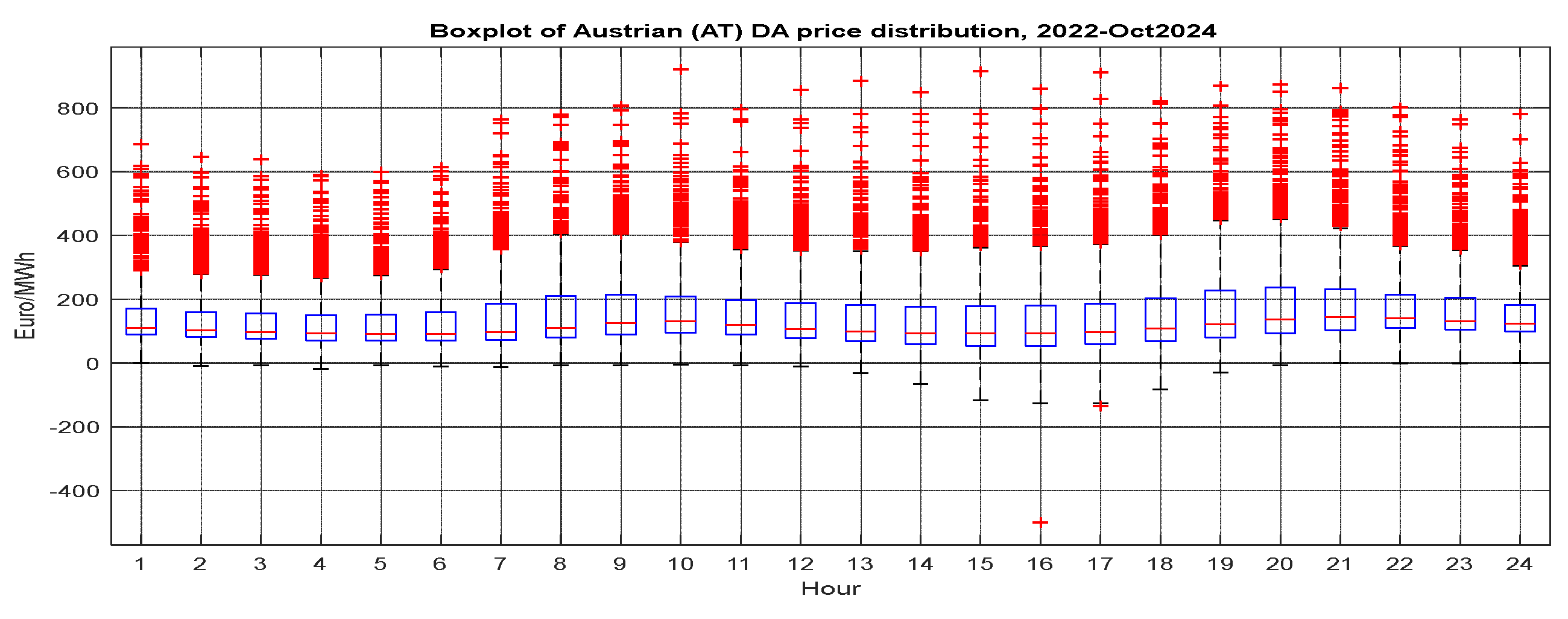
Figure 8.
Box plot of the distribution of the Romanian (RO) DA prices, 2022-Oct2024.
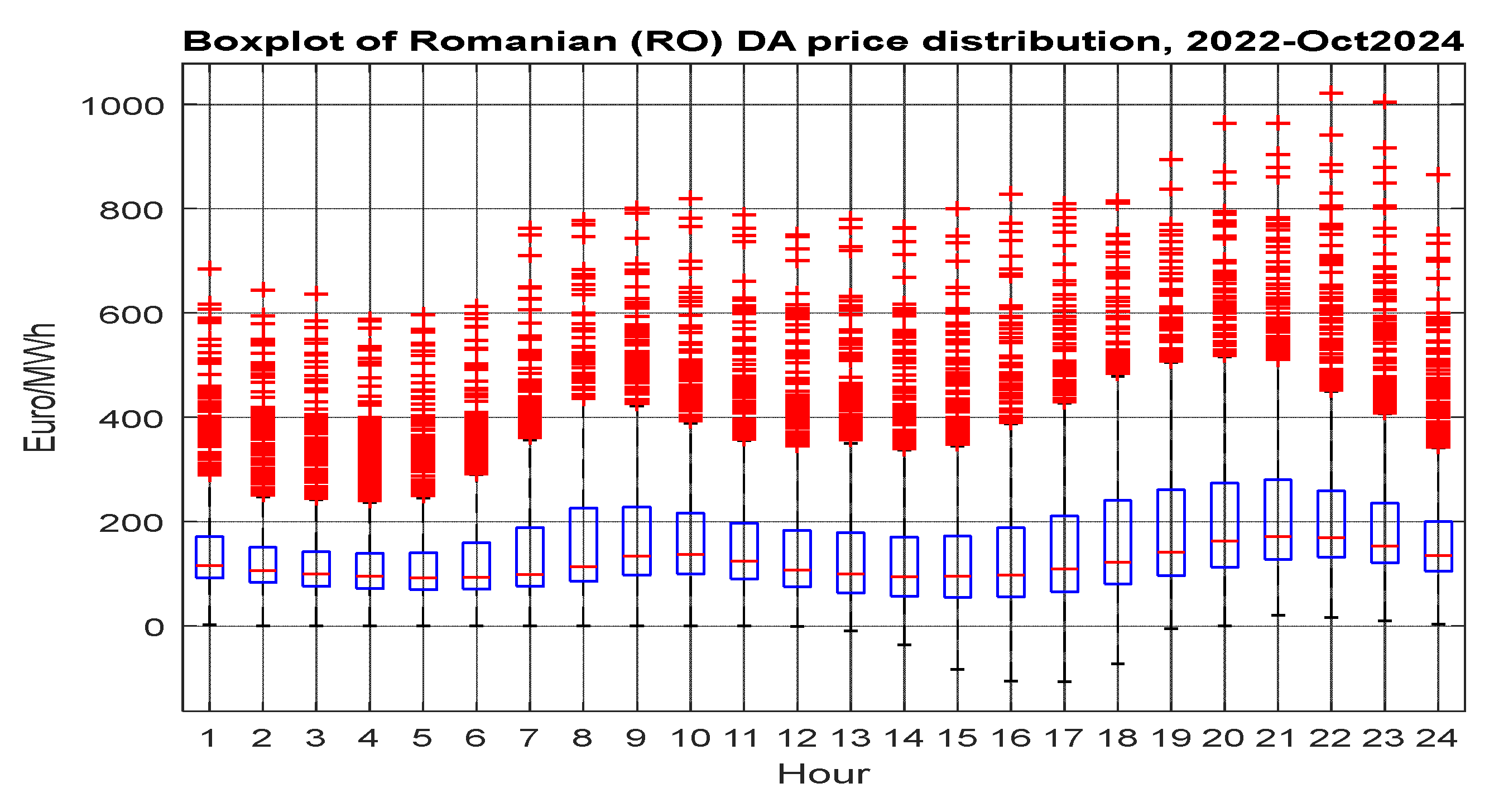
Figure 12.
A schematic representation of Causal feature selection and discovery, used in this work.
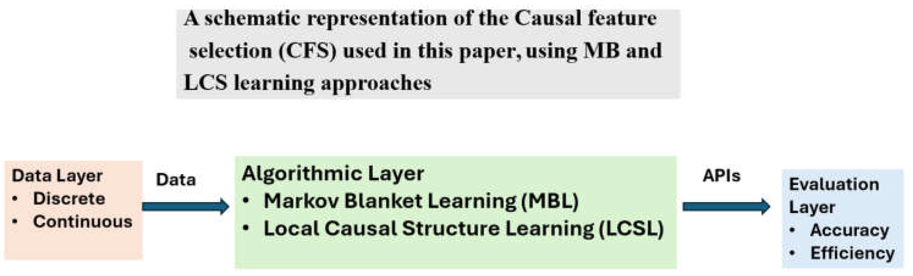
Figure 16.
Rolling volatility of AT, BG, GR, and HU DA prices using a window of 720 hours (month).
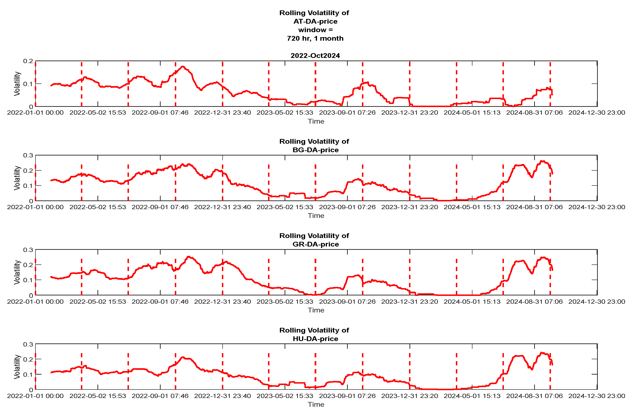
Figure 17.
Rolling volatility of ITS, RO and SI DA prices using a window of 720 hours (month).
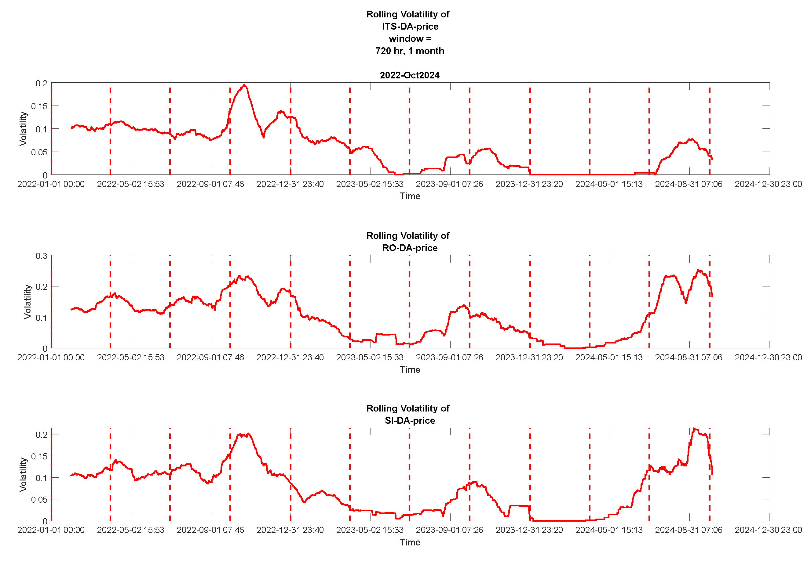
Figure 18.
Rolling volatility of AT-CH, AT-CZ, AT-DE Cross Border Transfer Availability (CBTA) using a window of 720 hours (month).
Figure 18.
Rolling volatility of AT-CH, AT-CZ, AT-DE Cross Border Transfer Availability (CBTA) using a window of 720 hours (month).
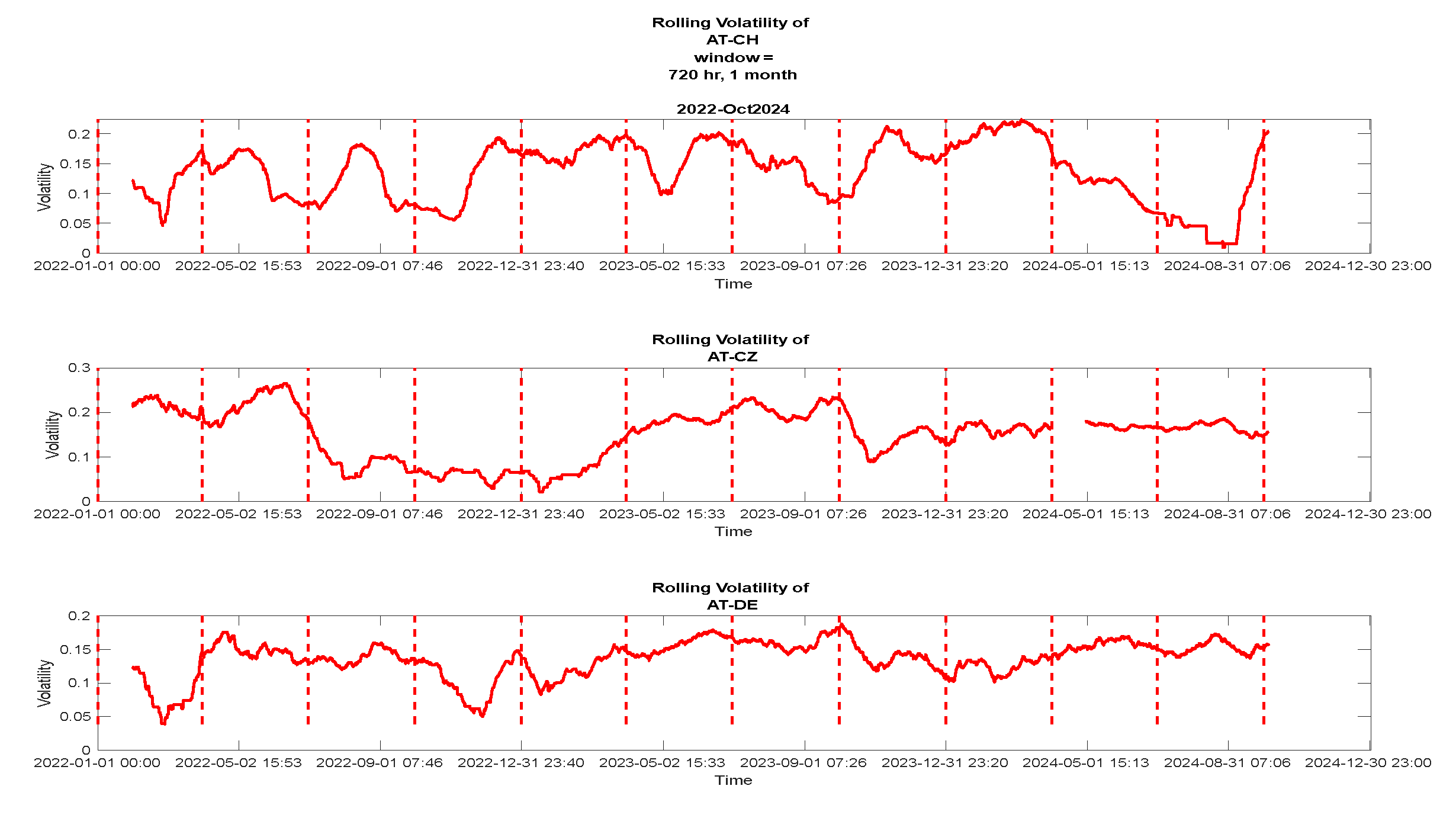
Figure 19.
Rolling volatility of AT-ITNorth, AT-Sl, AT-HU Cross Border Transfer Availability (CBTA) using a window of 720 hours (month).
Figure 19.
Rolling volatility of AT-ITNorth, AT-Sl, AT-HU Cross Border Transfer Availability (CBTA) using a window of 720 hours (month).
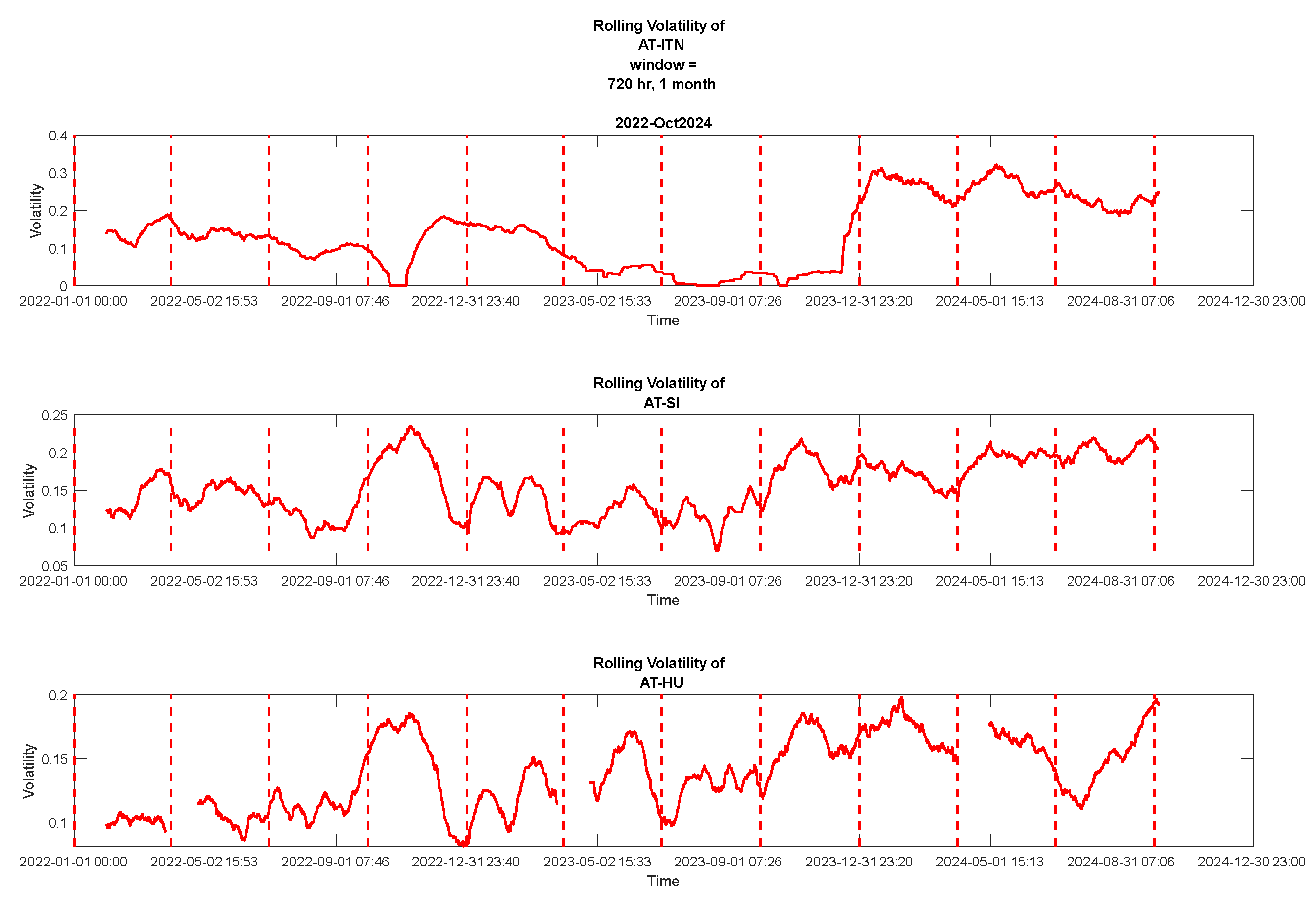
Figure 20.
Correlation of rolling volatility curves of all DA prices and CBTA using a window of 720 hours (month).
Figure 20.
Correlation of rolling volatility curves of all DA prices and CBTA using a window of 720 hours (month).
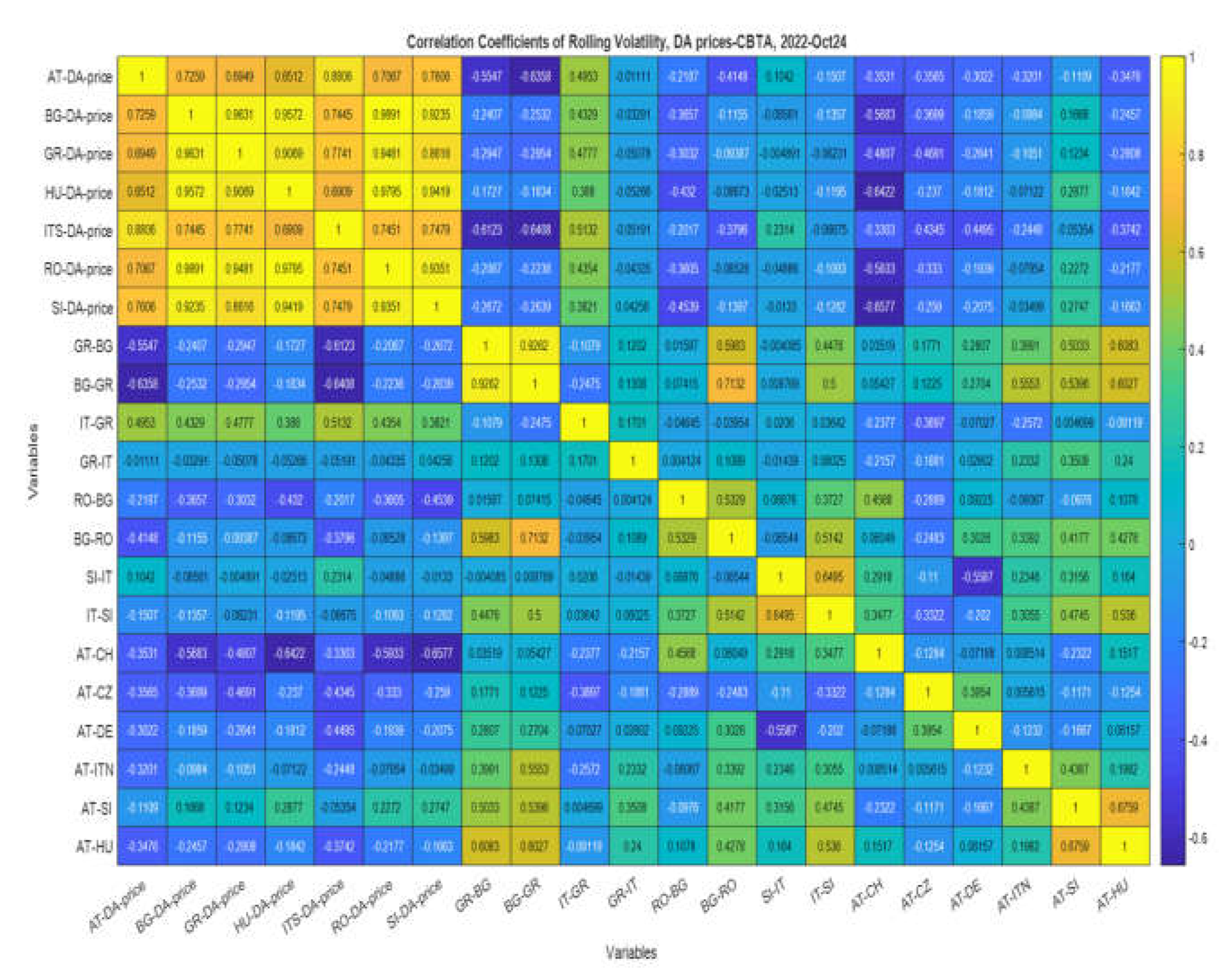
Figure 22.
Physical and commercial flows diagram, 2023-2024.
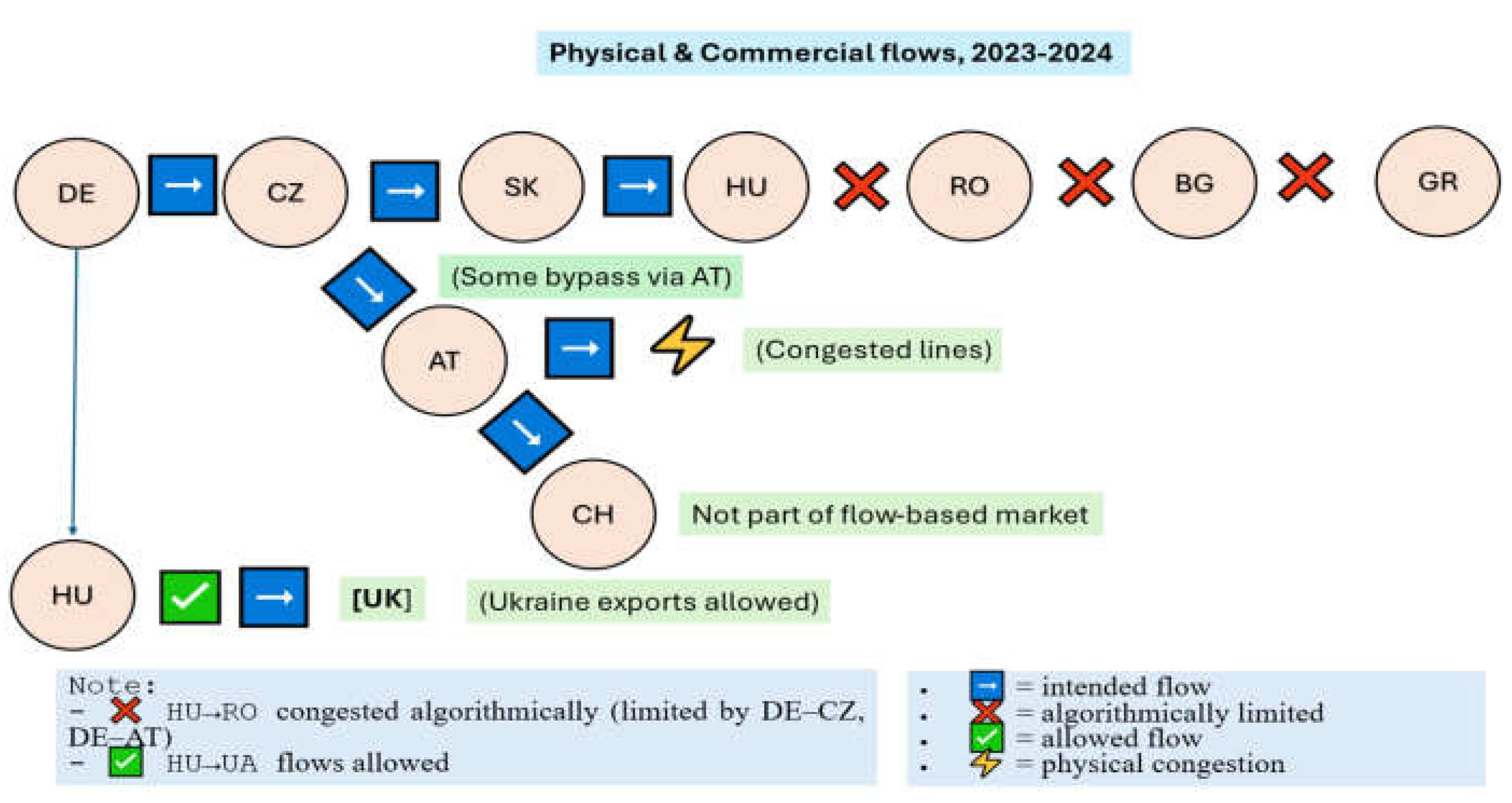
Table 8.
Summary of differences of AT and RO spot hourly price boxplots .
| Aspect | Austria (AT) | Romania (RO) |
|---|---|---|
| Median Prices | Lower (~100–200 EUR/MWh) | Higher (~200–300+ EUR/MWh) |
| Volatility | Lower | Higher |
| Outliers | Present but moderate | Frequent and extreme (>1000 EUR/MWh) |
| Negative Prices | Occasionally present | None observed |
| Peak Price Hours | Mornings and evenings | Spikes during mornings and especially evenings |
| Market Behavior | More stable and flexible | Higher stress and supply volatility |
Table 9.
Aggregated summary statistics for market comparison (per market analysis).
| Market | avgPrice | medianPrice | St.Dev | IQR | minPrice | maxPrice | CV | Peak-Off-Peak Spread (PoPS) |
Extreme-FreqPct | skewness | kurtosis |
|---|---|---|---|---|---|---|---|---|---|---|---|
| AT | 151.067 | 111.315 | 122.897 | 110.645 | -500.000 | 919.640 | 0.814 | 59.608 | 9.995 | 1.841 | 7.233 |
| BG | 154.763 | 119.295 | 119.108 | 114.435 | -45.000 | 950.010 | 0.770 | 94.164 | 9.995 | 1.802 | 7.339 |
| GR | 170.618 | 130.650 | 117.579 | 130.290 | -1.020 | 942.000 | 0.689 | 76.433 | 9.999 | 1.604 | 6.496 |
| HU | 161.898 | 120.970 | 128.535 | 119.975 | -500.000 | 1047.100 | 0.794 | 86.169 | 9.999 | 1.811 | 7.179 |
| ITS | 180.862 | 134.070 | 120.720 | 115.925 | 0.000 | 870.000 | 0.667 | 59.204 | 9.999 | 1.842 | 6.816 |
| RO | 159.411 | 119.750 | 128.138 | 117.520 | -106.360 | 1021.610 | 0.804 | 95.312 | 9.999 | 1.849 | 7.267 |
| SL | 159.725 | 117.910 | 126.317 | 120.660 | -500.000 | 1022.270 | 0.791 | 74.068 | 9.999 | 1.757 | 6.853 |
| Note: IQR : interquartile range, CV: Coefficient of Variation=std/mean, PoPS: Peak-off-peak spread i.e. avg price (7-10pm) - avg price (2-5am), Extreme-Freq Pct : frequency of extreme prices (%>90th percentile) | |||||||||||
Table 10.
Average and total (across all hours) number of hourly price outliers.
| Market | Average Number of Outliers |
Total Number of Outliers |
|---|---|---|
| AT | 20.13 | 483 |
| BG | 26 | 630 |
| GR | 31 | 767 |
| HU | 27.1 | 651 |
| ITS | 30.5 | 733 |
| RO | 28 | 672 |
| SI | 24.6 | 592 |
Table 12.
List of algorithms associated with Markov Blanket (MB), Global and Local Causal Structure Learning (GCS-LCS).
Table 12.
List of algorithms associated with Markov Blanket (MB), Global and Local Causal Structure Learning (GCS-LCS).
| Global Causal Structure Learning (GCS) algorithms | ||
|---|---|---|
| Acronym | Title of algorithm | Reference |
| GSBN | Grow/Shrink Bayesian network | [35] |
| GES | Greedy Equivalence Search | [53] |
| PC | PC | [21] |
| MMHC | Max-Min Hill-Climbing | [32] |
| PCstable | PC-stable | [43] |
| F2SL_c | Feature Selection-based Structure Learning using independence tests | [6] |
| F2SL_s | Feature Selection-based Structure Learning using score functions | [6] |
| Local Causal Structure (LCS) learning algorithms | ||
| PCDbyPCD | PCD-by-PCD | [42] |
| MBbyMB | MB-by-MB | [44] |
| CMB | Causal Markov Blanket | [18] |
| LCSFS | Local Causal Structure Learning by Feature Selection | [19] |
| Markov blanket (MB) learning algorithms | ||
| GS | Grow/Shrink algorithm | [35] |
| IAMB | Incremental Association-Based Markov Blanket | [45] |
| InterIAMB | Inter-IAMB | [36] |
| InterIAMBnPC | Inter-IAMBnPC | [32] |
| FastIAMB | Fast-IAMB | [37] |
| FBED | Forward-Backward selection with Early Dropping | [46] |
| MMMB | Min-Max MB | [45] |
| HITONMB | HITON-MB | [47] |
| PCMB | Parents and children-based MB | [48] |
| IPCMB | Iterative Parent-Child based search of MB | [9] |
| MBOR | MB search using the OR condition | [49] |
| STMB | Simultaneous MB discovery | [50] |
| BAMB | Balanced MB discovery | [51] |
| EEMB | Efficient and Effective MB | [52] |
| MBFS | MB by Feature Selection | [51] |
Table 13.
Possible interpretations of high and low correlation of volatilities between two markets.
| Conditions* | Interpretation |
|---|---|
| Markets share weather patterns | Likely weather-driven common volatility (hydro/wind output variability) |
| Markets are strongly interconnected | Likely volatility transmission via power flows/coupling mechanisms |
| Markets have similar generation mixes | Fuel-driven spillovers (e.g., gas price shocks affect both) |
| *Note: Real examples of market conditions are the results in Figure 24 and Table 13, in the results section. | |
Table 14.
Relating spot price volatility correlation patterns with structural asymmetries.
| Scenario | Implication |
|---|---|
| Market A has persistent high volatility, and others show delayed rise | A is likely a volatility transmitter |
| Market A is small but strongly correlated with a larger hub | Possibly price-taking market with imported volatility |
| Markets with weak coupling show weak correlation | Physical/market coupling is crucial for volatility transmission |
Table 15.
Results of the Local Causal Structure Learning (LCSL) using the CMB algorithm.
| Local Causal structure learning LCSL: algorithm CMB | |||
| Target Variable: AT-DA-p (1*) | |||
| Year | 2022 | 2023 | 2024 |
| Parents Children Spouses |
63, 64 24, 32, 47, 66 - |
5, 24, 47, 58, 60, 64 4, 39 - |
5, 6, 7, 22, 27, 31, 35, 47, 53, 54, 64 - - |
| Target Variable: BG-DA-p (7) | |||
| Parents Children Spouses |
1, 6, 15, 19, 35, 39, 42 46 - - |
5, 15, 31, 52, 60, 66 28, 39 - |
24, 39 15, 21, 50 - |
| Target Variable: GR-DA-p (15) | |||
| Parents Children Spouses |
7, 19, 32, 39,47 22, 44 - |
7, 10, 14, 19,22,32,37,54 - - |
7, 19, 20, 32, 39, 45, 46 5 - |
| Target Variable: HU-DA-p (24) | |||
| Parents Children Spouses |
1, 18, 39, 43 47 - |
1, 13, 22, 25, 29, 39, 47,52 - |
39 7, 27,29,43,47, 55 - |
| Target Variable: ITS-DAp (32) | |||
| Parents Children Spouses |
7, 61 1,10,15,23,30,36,47,56,60,63 - |
5, 7,15,29,35,36,47,52,63 25 - |
1,15, 18,36,38,47 35, 58, 62 - |
| Target Variable: RO-DAp (39) | |||
| Parents Children Spouses |
7,15,24,43,56 62, 67 - |
1,5,7,35 24 - |
7,15,24,47 23, 43 - |
| Target Variable: SI-DAp (47) | |||
| Parents Children Spouces |
1,12,38 24, 32, 64 |
31, 35 1, 24, 39, 65 - |
32, 38 1, 7, 24, 37, 50 |
| Notes: for the full name of nodes & description, see Table 1. Numbers in bold indicate variables included in the Markov Blanket (MB) but now equipped with direction arrows. * Indicate the number of the variable in Table 1. | |||
Table 17.
provides a short visual summary of the figure above. Short visual summary.
| From | To | Flow Status | Reason |
|---|---|---|---|
| DE → CZ → HU → RO | BG | Limited (❌) | Congestion upstream (DE–CZ, AT) |
| HU → UA (Ukraine) | Allowed (✅) | Lower congestion impact | |
| DE/AT → CH | No market coupling (⚡) | Switzerland outside EU market |
Table 18.
Detailed evaluation of the performance of the European TM, in the case of SEE spot price surge.
Table 18.
Detailed evaluation of the performance of the European TM, in the case of SEE spot price surge.
| Aspect | Result in 2023–24 | Comments |
|---|---|---|
| Price convergence | ❌ Failed | Prices in SEE diverged strongly from Core (DE/AT/CZ) |
| Grid physical realism | ✅ Worked | FBMC realistically modeled grid congestions |
| Market integration | ❌ Partially failed | SEE countries were semi-isolated |
| Security of supply | ✅ Generally OK | No blackouts, but expensive |
| Efficient capacity use | ❌ Not optimal | Some capacities underused (especially HU→RO) |
Disclaimer/Publisher’s Note: The statements, opinions and data contained in all publications are solely those of the individual author(s) and contributor(s) and not of MDPI and/or the editor(s). MDPI and/or the editor(s) disclaim responsibility for any injury to people or property resulting from any ideas, methods, instructions or products referred to in the content. |
© 2025 by the authors. Licensee MDPI, Basel, Switzerland. This article is an open access article distributed under the terms and conditions of the Creative Commons Attribution (CC BY) license (http://creativecommons.org/licenses/by/4.0/).
Copyright: This open access article is published under a Creative Commons CC BY 4.0 license, which permit the free download, distribution, and reuse, provided that the author and preprint are cited in any reuse.


