
Submitted:
15 July 2025
Posted:
22 July 2025
You are already at the latest version
Abstract
This study introduces a Spatio-Temporal Graph Attention Network (STGAT) for non-stationary financial systems to address challenges in stock price prediction, such as non-stationarity and complex dependencies, by integrating a gated causal temporal convolution module and a novel graph attention module. STGAT employs causal time-modeling to prevent future information leakage, a dynamic industry-correlation graph attention mechanism for adaptive weight learning, and a multi-scale MIMO framework for industry-grouped feature extraction. Its symmetric integration of temporal and spatial modeling balances time-series dynamics with inter-stock correlations. Experiments on the New York Stock Exchange’s commercial banking and metals sectors demonstrate that STGAT substantially outperforms XGBoost, LSTM, and SARIMA in predictive accuracy, particularly in high-volatility scenarios. This research underscores the efficacy of graph neural networks in modeling interconnected financial systems and offers insights for advancing portfolio optimization and risk management.
Keywords:
STGAT
; stock price prediction
; spatio-temporal graph neural network
; graph attention network
; causal convolution
; financial market modeling
MSC: 68T07; 68R10; 91G45
1. Introduction
In the dynamic evolution of financial markets, stock price forecasting has always been a core issue in theoretical research and practical applications [1]. Its importance is not only reflected in its value as a guide for investors’ personal asset allocation, but also as a key basis for financial institutions’ risk management, asset pricing, and investment strategy formulation. Accurate stock price forecasting can help investors capture potential gains from market fluctuations and avoid systemic risks. However, forecasting activities are complex and subject to many uncertainties [2], making understanding future stock prices extremely challenging.
Traditional stock price prediction methods, such as ARIMA models and statistical regression analysis [3], are constrained by linearity assumptions and the requirement of data smoothness, making them inadequate for capturing the inherent complexity and non-stationarity of financial markets. Stock prices are subject to abrupt fluctuations driven by macroeconomic policies, earnings announcements, geopolitical events, and other external shocks, resulting in pronounced non-linear dynamics and volatility clustering that traditional models struggle to represent effectively.
While machine learning approaches [4] overcome some linearity limitations, they often depend on handcrafted features and lack the capacity to model intricate inter-stock relationships or adapt to evolving market structures, thus limiting their generalizability and robustness. Consequently, these traditional and machine learning methods frequently fall short in delivering accurate, reliable, and timely stock price forecasts.
The booming development of deep learning has brought revolutionary breakthroughs to financial market analysis [5]. Among them, the Recurrent Neural Network (RNN) [6] and its classic variant, the Long Short - Term Memory network (LSTM) [7], can capture the dynamics of stock prices in the time dimension with their sequence modeling capabilities. The RNN realizes the modeling of temporal dependencies through the recurrent connection of the hidden layer. However, in scenarios with long - distance dependencies, the problem of gradient vanishing is significant. In contrast, the LSTM effectively solves the long - term memory bottleneck of the traditional RNN through the gating mechanism composed of the forget gate, input gate, and output gate.
However, complex correlations among stocks in the financial market (such as industry linkages and sector rotations) urgently require more efficient structured modeling tools. Thus, Graph Neural Networks (GNNs) have become a new paradigm [8]. GNNs naturally represent the dependency relationships among stocks through the topological structure of nodes and edges, and can effectively capture non - Euclidean space correlations such as upstream and downstream of the industrial chain and sector collaboration.
Based on this, Spatio - Temporal Graph Attention Networks (STGATs) [9] further integrate time - series dynamics and graph - structure representation. Through the attention mechanism, they adaptively focus on key nodes and temporal patterns. This not only breaks through the limitations of traditional methods in spatial correlation modeling but also strengthens the ability to fuse multi - scale spatio - temporal features, providing a highly promising solution for improving the accuracy and robustness of stock price prediction.
This paper proposes a spatio-temporal graph attention network (STGAT) for non-stationary financial systems, and builds a set of spatio-temporal adaptive prediction framework specifically designed for stock price prediction, and achieves technological innovation in Spatial Temporal Modeling and Model Architecture, the following are the main innovations:
- Causal Temporal Modeling Mechanism The Gated Causal Convolution network is adopted, strictly following the causal constraints of financial time series to avoid the leakage of future information.
- Dynamic Industry Association Graph Attention Model An adaptive graph attention architecture that integrates industry rotation factors is constructed. Through the edge - attribute attention mechanism of GATv2, the association weights between financial entities are dynamically learned. The model takes industry classification information and market correlation matrices as edge - attribute inputs, and through the attention mechanism, it automatically distinguishes the true associations driven by industry fundamentals from the false correlations caused by market sentiment.
- Multi - scale Industry Sector MIMO Framework A multi - input multi - output prediction architecture based on industry sectors is designed, breaking through the limitations of single - asset independent modeling. Through the industry grouping mechanism, homogeneous financial entities are clustered into sub - graphs, and the graph attention layer is used to capture the intra - group synergy and inter - group transmission relationships.
In an empirical study of the commercial banking and energy sectors of the New York Stock Exchange, the STGAT model demonstrates significantly more predictive power than traditional benchmark models such as SARIMA, LSTM, and XGBOOST. The central innovation of this study is that it rejects the traditional view of stocks as isolated individuals and instead models the stock market as an interconnected network. This network-based perspective contributes to a deeper understanding of how various relational factors affect stock prices.
This research not only expands the methodological boundaries of financial forecasting but also demonstrates the strong potential of graph neural networks in modeling complex financial systems. The findings provide important theoretical support and practical guidance for portfolio optimization, risk management, and other financial applications, and are expected to promote further development of quantitative analysis and decision support in the field of finance.
2. Literature Review
Early financial forecasting primarily relied on traditional statistical models. The ARIMA model [10], while effective for modeling smooth time series and applied to stock price forecasting [11], is limited by its linear assumptions and inability to handle the non-stationarity and abrupt changes common in financial markets. To address volatility, Engle introduced the ARCH model [12], later extended to GARCH by Bollerslev [13], which models volatility clustering. However, these models remain constrained by their linear frameworks and cannot fully capture the complex nonlinear relationships in financial data.
With the advent of machine learning, models such as support vector machines (SVMs) [14] and random forests [15] enabled the modeling of nonlinear patterns in time series data. Despite this advancement, these methods heavily depend on manual feature engineering, requiring domain expertise and limiting their generalizability and scalability.
The advent of deep learning has significantly advanced time series modeling. LSTM, proposed by Hochreiter and Schmidhuber [16], addresses the gradient vanishing/exploding issues in RNNs through gating mechanisms, enabling the capture of long-range dependencies. In financial forecasting, LSTM has demonstrated strong potential for modeling long-term correlations [17]. Temporal Convolutional Networks (TCN) [18] utilize dilated convolutions to expand the receptive field and support parallel computation, improving efficiency over traditional RNNs and making them suitable for low-latency scenarios such as high-frequency trading. WaveNet [19] employs causal convolutions to ensure temporal causality and prevent information leakage from the future, setting a benchmark for time series modeling. However, these models primarily focus on single-sequence data and struggle to capture cross-asset or spatial relationships, underscoring the need for approaches that can model complex dependencies across multiple sequences.
The rise of graph neural networks (GNN) is naturally adapted to the financial market "entity association network " features (e.g., stock industry chain associations, institutional position networks, and credit bond collateral relationships): the basic GCN proposed by Kipf & Welling [20] pioneered the graph convolution operator to achieve node information propagation. These techniques draw from cluster analysis for non-stationary climate classification and AI models for extreme temperature forecasting, providing insights into handling financial spatio-temporal dependencies in STGAT [21,22]. GAT proposed by Velickovic et al. [23], which introduces an attention mechanism to dynamically allocate neighbour node weights and accurately identify association strength differences; GATv2 optimized by Brody et al. [24], which improves dynamic attention-computational logic, becomes the current state-of-the-art architecture in the field of graph learning.
In order to break through the modelling limitations of a single model and single variable in financial and other scenarios, the researchers also tried to build hybrid models with multivariate inputs by combining multiple deep learning and classical models.
Spatio - Temporal Graph Neural Networks (STGNN) focus on the "spatio - temporal coupling" characteristics of financial data, and fill the research gap through spatio - temporal joint modeling. In the field of traffic flow prediction, Yu et al. [9] proposed STGCN which pioneered the fusion architecture of graph convolution and 1D - CNN to depict spatio - temporal dependencies, and Wu et al. [25] proposed Graph WaveNet which introduced an adaptive adjacency matrix to dynamically capture time - varying spatial correlations, laying the foundation for technology transfer in financial scenarios. In terms of financial application exploration, Sawhney et al. [26] proposed STHAN - SR which integrated spatio - temporal attention mechanisms and hypergraph structures to adapt to complex financial correlations, attempting to depict the dynamic interactions of the asset network.
Kanwal et al. [27] proposed a hybrid deep learning model, BiCuDNNLSTM-1dCNN, integrating CUDA-accelerated bidirectional LSTM and one-dimensional CNN to capture both long-term temporal dependencies and short-term local patterns in stock price time series, demonstrating superior prediction accuracy across five datasets compared to four state-of-the-art models, although noting limitations in data scale dependency and hyperparameter optimization complexity.
Jin [28] proposes GraphCNNPred, a hybrid model integrating graph neural networks (GAT/GCN) and convolutional neural networks (CNN), which leverages feature correlation graphs and temporal convolutional layers to predict trends in stock market indices (S&P 500, NASDAQ, etc.), achieving a 4%-15% improvement in F measure over baseline algorithms and demonstrating effective trading strategy performance with a Sharpe ratio exceeding 3.
Liu and Paterlini [29] proposed an LSTM-GCN model that integrates a graphical convolutional network (GCN), which is used to capture spatial dependencies in supplier-customer value chain relationships, and a long- and short-term memory network (LSTM), which is used to simulate the temporal dynamics of stock returns in relation to the Euro Stoxx 600 Index and the S&P 500 Index. The model improves forecast accuracy and risk-adjusted returns compared to the baseline model for the Euro Stoxx 600 and S&P 500 datasets.
Wenbo Yan and Ying Tan [30] propose a time-correlation graph pre-training network TCGPN, which integrates time series and node dependencies through a time-correlation fusion encoder, combines self-supervised time-completion and semi-supervised graph recovery tasks to optimise representations, and solves the problem of large-scale node memory by using a node/graph/time-masked data augmentation strategy, which has been proposed in CSI300/Performance breakthroughs in non-periodic time series forecasting on CSI300/ CSI500 stock datasets with lightweight MLP fine-tuning.
Currently, there are several aspects of financial prediction models that can be optimized. In the causal constraint dimension, traditional convolution faces the problem of future data leakage [9], while RNN models encounter obstacles in parallelization, which negatively affects both the reliability and efficiency of forecasting. Second, in terms of dynamic relationship modeling, traditional methods rely excessively on static graph structures and have a single source of correlation, limited to the use of price correlation or industry classification [28]. However, dynamic changes such as industry restructuring and black swan events occur frequently in financial markets, and the market environment is complex and volatile. Under such circumstances, forecasting models perform poorly in dealing with unexpected events and also ignore the interactions between stocks, especially those in the same industry sector. Furthermore, in terms of model magnitude, most of today’s models focus on a single stock or a single indicator, and rarely consider a specific industry sector or system level [27].
This paper proposes a spatio-temporal Graph Attention Network (STGAT) for non-stationary financial systems. It provides an innovative solution that combines logical self-consistency and market adaptability for stock price prediction.
3. Theory Fundamentals
3.1. Graph Theory and Graph Convolutional Networks
Graph theory provides the mathematical foundation for modeling graph-structured data [31]. In mathematics, a graph is denoted as , where the node set
represents entities, and the edge set E represents the relationships between entities. The adjacency matrix describes the connection strength between nodes, and the degree matrix D is a diagonal matrix with elements .
Graph Convolutional Networks (GCN) extend the convolution operation to graph structures via spectral or spatial domain methods [20]. Spectral domain GCN is based on the eigen decomposition of the graph Laplacian matrix
which maps signals from the spatial domain to the frequency domain for processing. For example, the simplified GCN layer proposed by Kipf and Welling is expressed as:
where (adding self-loops), is the degree matrix of , is the learnable weight matrix, and is the activation function. This approach implicitly captures dependencies between nodes through the adjacency matrix, enabling the propagation of features over the graph structure.
3.2. Convolutional Neural Network
Convolutional Neural Networks (CNNs) [32] were originally designed for processing grid-structured data such as images, with their core advantage lying in capturing local features through shared convolutional kernels. In time series processing, one-dimensional convolution (1D Conv) in CNNs extracts local patterns along the temporal axis through sliding windows, offering advantages of parameter efficiency and parallel computation.
The Temporal Convolutional Network (TCN) [18] extends CNNs for temporal modeling by introducing causal convolution and dilated convolution. Causal convolution ensures that the output at the current time step depends only on past inputs, satisfying the causality requirement for time series prediction. Dilated convolution expands the receptive field by setting a dilation factor d, enabling the kernel to capture longer-range temporal dependencies:
where K is the convolution kernel size and x is the input sequence. By stacking multiple dilated convolutional layers with exponentially increasing dilation factors, TCN efficiently captures long-term temporal patterns without increasing the number of parameters.
3.3. The Fusion of Spatio-Temporal Graph Convolutional Network
spatio-temporal Graph Convolutional Networks (STGCN) [9] integrate the advantages of graph theory and CNNs to simultaneously process spatial dependencies and temporal dynamics in data. The core concept of STGCN involves designing specialized spatio-temporal convolution modules that separately capture spatial relationships in graph structures and temporal evolution in sequential data.
In the spatial dimension, STGCN typically employs GCN or its variants (e.g., ChebNet, GAT) for graph structure modeling. In the temporal dimension, it utilizes CNNs (e.g., TCN) or RNNs (e.g., LSTM) to process temporal features. For instance, the STGCN framework proposed by Yu et al. decomposes spatio-temporal convolution into two sequential operations: spatial graph convolution and temporal convolution:
where denotes the spatial graph convolution operation, represents the temporal convolution operation, and and are learnable weights for spatial and temporal dimensions respectively. This decomposition enables the model to learn simultaneously node dependency relationships in space and evolution patterns in time.
4. STGAT: Model Structure and Innovation
This innovative architecture enables STGAT to simultaneously capture 1) long-term evolutionary trends and short-term volatility patterns in the time dimension, 2) complex market linkage effects in the spatial dimension, and 3) local features of unexpected market events.As such, it is expected to enhance the training of the model and is expected to produce good forecasting results.
We propose an innovative spatio-temporal graph attention network (STGAT) that aims to significantly improve the accuracy of stock price prediction while effectively capturing the complex spatio-temporal dependencies in financial markets.
The model we design contains two core components that work in tandem: a gated temporal convolution module and an augmented graph attention module, which together build a hierarchical feature extraction architecture. The former employs strict causal constraints and an innovative gating mechanism to capture long-term evolutionary patterns in the temporal dimension, preserving key features and suppressing noise, while the latter learns complex spatial relationships among stocks using a multi-attention mechanism, which adjusts the attention coefficients with the help of edge attributes.
The two modules work together through a “time-convolution-graph-attention-time-convolution” sandwich symmetry structure, and the model achieves hierarchical feature abstraction through a cascading spatio-temporal block architecture: the first block extracts the underlying spatio-temporal patterns, and the second captures the higher-order market dynamics. The final prediction layer generates accurate forecasts through feature fusion coupled with a fully connected network.
This innovative architecture enables STGAT to simultaneously capture 1) long-term evolutionary trends and short-term volatility patterns in the time dimension, 2) complex market linkage effects in the spatial dimension, and 3) local features of unexpected market events. As such, it is expected to enhance the training of the model and produce robust forecasting results.
Figure 1 illustrates the schematic of our model. This model architecture takes the spatio-temporal Graph Attention Network (STGAT) as the core. After the input data is processed by cascaded STGAT blocks, the output layer generates the results.
First, the Temporal ConvLayer, which contains causal gated convolution and residual feature fusion, is used to extract temporal patterns. Another temporal convolution layer is employed to fuse features. Residual connections within the temporal block further enhance feature propagation.
Subsequently, the GATv2 layer, equipped with dynamic attention and query - awareness capabilities, learns complex spatial relationships among stocks. Within the spatial block, operations such as GATv2, ReLU, BN layer, and Dropout are configured to effectively capture the spatio-temporal dependencies of financial data.
The combination of causal convolution and gating mechanisms (Sigmoid, Hadamard Product) optimizes information transmission, enabling hierarchical feature abstraction and accurate prediction.
4.1. Temporal Convolutional Layer
Building on the traditional TCN framework, which uses causal convolution to ensure temporal causality and dilated convolution to capture long-range dependencies, the temporal convolution layer introduces a dual-branch structure integrating gating mechanisms and residual connections. This design maintains TCN’s ability to model dynamic temporal dependencies while enhancing the focus on key temporal patterns through the gating mechanism, addressing the challenge of inadequate attention to local critical information in non-stationary sequences in traditional TCNs.
- Causal Conv: Causal convolution [33] is the core operation of the temporal convolutional layer. It strictly adheres to temporal causality, ensuring that the output at each time step depends solely on historical and current inputs, excluding future data. This design supports accurate forecasting in tasks such as time-series prediction and action segmentation.
-
Gating Mechanism: The Gated Linear Unit (GLU) [34] controls information flow through a gating mechanism, defined as:The input undergoes two linear transformations: one produces a feature vector, and the other generates a gating signal (0 to 1) via the Sigmoid function. The gating signal is element-wise multiplied by the feature vector to selectively filter relevant features. For efficiency, the input can be split along the feature dimension. GLU’s flexibility and variants enable its application to diverse tasks, enhancing the model’s ability to focus on critical information.This model leverages the Gated Linear Unit (GLU) to optimize temporal feature processing.The temporal convolution layer employs a dual-branch structure. One branch applies Sigmoid activation to the causal convolution output, generating a gating coefficient between 0 and 1 to regulate information flow. The other branch processes the causal convolution output to produce the main feature, which is gated by the coefficient via the Hadamard product and combined with the residual component.During feature fusion, the residual component is optimized to enhance effective temporal features. Residual connections stabilize training and preserve essential features, making this approach a spatio-temporal variant of the GLU mechanism.
4.2. Spatial Convolution Layer
The main function of the spatial convolution layer is to capture the features of data in the spatial dimension, that is, the relationships between nodes. Through the graph attention mechanism, it adaptively learns the importance among nodes, thereby better extracting the spatial information in graph-structured data.
-
GATv2: GATv2 (Graph Attention Network v2) [24] is an improved version of the traditional Graph Attention Network (GAT), and the core innovation is to solve the "masking bias" problem of the attention mechanism in the original GAT. Traditional GAT applies masks to invisible nodes (e.g. non-neighbour nodes) when calculating the attention weights, which leads to bias in the attention calculation process. GATv2, on the other hand, by redesigning the calculation of the attention mechanism, makes the model no longer rely on masks when calculating the attention weights, so that it can deal with all the nodes in a fairer way, and improves the model’s expressive and generalisation abilities. This optimization builds on advanced graph attention techniques, enhancing spatial relationship modeling in STGAT [35].The core operation of GATv2 is represented as follows:where and represent the feature vectors of nodes i and j, is a learnable weight matrix, and represents the attention mechanism.
- Explicit Edge Attributes: Traditional GATv2 [24] relies solely on node features, limiting its use of edge semantic information, graph structure, and domain knowledge. By incorporating edge attributes, such as industry correlation weights and stock relevance coefficients, into the GATv2 layer’s attention calculation, our model enhances domain knowledge integration and graph structure modeling. This approach dynamically adjusts attention weights, shifting from node-centered to edge-node synergistic modeling. It effectively addresses complex applications, such as financial modeling, where edge attributes carry rich semantic information.
4.3. Output Layer
The output layer of the STGAT model employs a hierarchical fully-connected architecture with a ReLU activation function, which maps the spatio-temporal features extracted by the previous STGAT module into task-specific predictions. The output layer consists of two consecutive "fully-connected - ReLU" layers followed by a final linear projection layer, which dynamically aggregates multi-scale temporal and spatial dependencies through a learnable weight matrix to efficiently transform high-dimensional graph structural features into predictions of future time steps.
5. Experimental Design and Process
Figure 2 illustrates the stock price analysis pipeline using the Spatio-Temporal Graph Attention Network (STGAT). The NYSE stock price dataset is preprocessed, including feature extraction, normalization, and graph structure construction, then split into training and test sets. The training set is processed through an input layer, stacked STGAT blocks, and an output layer for model training. The test set undergoes inference, followed by post-processing, enabling model evaluation and visualization to achieve spatio-temporal correlation-driven stock prediction.
5.1. Data Description
The dataset integrates New York Stock Exchange (NYSE) stock data (2000–2024) and Fortune 500 company data (2024), including ticker symbols and industry information. We merged the NYSE dataset with Fortune 500 industry details. Stocks were filtered based on consistent trading days and trade frequency to ensure data validity. Ultimately, 273 stocks with complete industry sector data were selected, forming a comprehensive dataset for spatio-temporal stock price analysis.
We select the following financial indicators:
- Basic trading indicators: Open, High, Low, Close, Volume
- Technical indicators: EMA (Exponential Moving Average), RSI_14 (Relative Strength Index with 14-day period)
- Daily return: Return
5.2. Data Processes
Below is an overview of our experimental process, covering data preprocessing, fitting the data into a deep learning (DL) model, and finally evaluating the trained model.
All numerical features are normalized using Min-Max scaling to the range [0, 1]:
This mitigates the impact of different feature scales on model performance.
Temporal samples are generated using a sliding window approach with window size :
- Each window contains features from to t
- The label for each window is the target value at time
- If future data is unavailable, the label is set to 0
The sampling process can be formalized as:
where denotes the feature vector at time t, and is the corresponding label.
5.3. Graph Structure Construction
This graph structure integrates spatial and temporal dependencies through a three-stage process as following. The approach enhances stock relationship modeling by incorporating matching preclusion principles for robust graph connectivity [36,37].
5.3.1. Node Feature Construction
Nodes are composed of stocks with complete trading dates on the New York Stock Exchange. Each node feature includes numerical features such as opening price, highest price, lowest price, closing price, trading volume, EMA, RSI_14, and Return. After MinMax normalization, time series information is extracted through a sliding window of size 10. The window data is used as the node input, and the target value of the corresponding next time step is used as the label. Finally, all node data is integrated through tensor operations to form a four - dimensional tensor structure of [number of samples, number of nodes, time steps, number of features].
5.3.2. Spatial Edge Construction
We define two types of edges to model spatial relationships. For each pair of nodes and , their final edge weight is computed as the sum of individual edge weights from different relationship types:
- Industry-based Edges: Encode domain prior knowledge. Stocks in the same sector are connected with a fixed weight of :
- Correlation-based Edges: Data-driven edges computed from Pearson correlation coefficients of daily closing prices:where is the Pearson correlation coefficient between the closing prices of and .
The combined edge weight between nodes and is:
All edges are undirected, enforced by adding reciprocal pairs and to ensure the symmetry of the graph convolution operation.
5.3.3. Temporal Extension
The spatial edge set is replicated across time steps within the sliding window. For each time step t (, where is the window size), node indices are offset by (N is the number of stocks) to distinguish nodes across time:
Temporal edges are constructed by replicating spatial edges at each time step with preserved weights:
The final spatio-temporal edge set is:
This process fuses spatial connectivity with temporal dynamics, forming a structured input for spatio-temporal graph neural networks.
Algorithm 1 shows the logic of spatial edge construction and temporal expansion.
| Algorithm 1: Spatio-temporal Graph Construction |
|
Input: Industry information I, Price correlation matrix C, Window size w, Number of stocks N
Output: Spatio-temporal edge set E with combined weights
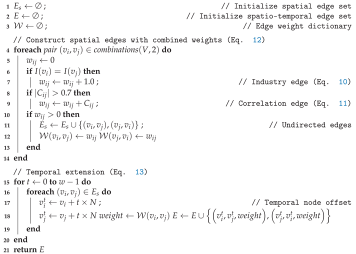
|
5.4. Experimental Setup and Evaluation
The training framework is implemented using a custom trainer (CustomTrainer), integrating data partition, model optimization, and performance evaluation. Key configurations are as follows:
5.4.1. Data Partition and Optimization Strategy
Data Partition: The dataset is partitioned into training and test sets at a 9:1 ratio, with the test set used to evaluate model generalization.
Optimizer: The Adam optimizer is employed with the following configurations:
- Learning rate:
- Weight decay:
- AMSGrad variant enabled for training stability.
Batch Processing: A batch size of 512 is used, with efficient data loading and shuffling implemented via .
5.4.2. Loss Function and Evaluation Metrics
Loss Function: The Mean Squared Error (MSE) is used as the optimization objective:
where and denote the ground truth and predicted values, respectively, and n is the number of samples.
Evaluation Metric: The Root Mean Square Error (RMSE) is consistent with the unit of the ground truth, providing an intuitive measure of average prediction. It is defined as:
The Mean Absolute Error (MAE) is a pivotal regression evaluation metric that quantifies the average magnitude of prediction errors without considering their direction. Mathematically, it is defined as:
5.5. Comparison Models in the Experiment
In order to evaluate the performance of the Spatiotemporal Graph Attention Network (STGAT) model proposed in this study, we compare it with the traditional Autoregressive Integrated Moving Average model (SARIMA), Long Short-Term Memory network (LSTM), and Gradient Boosting Tree model (XGBoost).
- SARIMA: As a classic time series analysis method, SARIMA performs well in handling data with seasonality and trend. The model structure constructed based on statistical principles can effectively capture the internal laws of the data.
- LSTM: As a powerful recurrent neural network, LSTM solves the problems of gradient vanishing and gradient explosion in traditional recurrent neural networks by introducing a gating mechanism, and can better handle the dependency relationships in long - sequence data.
6. Experimental Results and Analysis
As mentioned before, we will start from the relatively macro perspective of industry sectors to study the stock prediction effect of the model. In the experiment, we take two different stock industry datasets as examples, namely the commercial bank dataset and the energy industry dataset. We report the research results in the following two subsections. First, regarding the commercial banks sector, and second, the metal sector.
6.1. Performance on Commercial Banking Sector
To evaluate the forecasting performance of models for commercial bank share prices, we compare STGAT, XGBoost, LSTM, and SARIMA across 15 banks, using root-mean-square error (RMSE) and mean absolute error (MAE) as primary metrics. We derive key observations from Figure 3 and Figure 4, highlighting their predictive accuracy.
Combined with the bar chart and experimental data, in the task of commercial bank stock price prediction, the STGAT model shows significant advantages.
Using mean absolute error (MAE) and root mean square error (RMSE) metrics, STGAT consistently outperforms XGBoost, LSTM, and SARIMA across 15 banks in high-volatility scenarios (e.g., GS and JPM) and stable scenarios (e.g., RF). For GS bank, STGAT achieves an MAE of 23.39 and RMSE of 33.58, substantially lower than XGBoost (MAE 114.61, RMSE 117.77) and LSTM (MAE 75.55, RMSE 89.51), highlighting its ability to capture complex volatility patterns.
Stock price volatility varies significantly across banks, with higher errors for high-volatility banks (e.g., GS, JPM) and lower errors for low-volatility banks (e.g., RF) across all models. STGAT maintains low MAE and RMSE across diverse volatility conditions, demonstrating superior robustness and adaptability compared to other models, thus confirming its effectiveness for stock price prediction.
Comparing the predicted and original stock prices of four models is highly informative for commercial bank stock price prediction. Figure 5 and Figure 6 plot the original and predicted stock prices for the models on commercial bank stocks KEY and RF, illustrating their forecasting accuracy over time.
In Figure 5, STGAT’s root-mean-square error (RMSE, approximately 1.57) is 15–32% lower than XGBoost’s (2.28), LSTM’s (1.83), and SARIMA’s (2.11), demonstrating superior predictive accuracy.
For KEY stock, STGAT accurately captures inflection point slopes during the 2023 Q2 downturn (18 to 12) and early 2024 rebound (10 to 15). In contrast, XGBoost exhibits step-wise fitting errors due to piecewise linear modeling, and SARIMA fails to capture nonlinear rebounds due to its linear assumptions. This highlights STGAT’s ability to effectively model time-series structures, achieving significant improvements in volatile scenarios through its architecture.
In Figure 6, RF stock prices exhibit moderate stability with narrow fluctuations and consistent trends. STGAT’s RMSE (approximately 4.89) surpasses XGBoost (5.27), LSTM (5.49), and SARIMA (6.32). STGAT precisely captures short-term inflection points, e.g., the March 2022 pullback (1–2 trading days earlier than XGBoost), and aligns closely with actual prices in smooth sequences, avoiding SARIMA’s underestimated trends and XGBoost’s slope distortions. This confirms STGAT’s robust adaptation to dynamic trends in moderately stable scenarios via spatio-temporal correlation modeling.
6.2. Performance on Metal Sector
To further evaluate model generalization for stock price prediction in the energy sector, we compare STGAT, XGBoost, LSTM, and SARIMA across six energy companies. Figure 7 and Figure 8 present key observations, highlighting their predictive performance.
Model errors vary significantly across metals sector stocks, e.g., AA, CLF, and RS, reflecting how individual stock volatility affects prediction difficulty.
For most stocks, such as AA and CMC, STGAT achieves lower RMSE and MAE than XGBoost, LSTM, and SARIMA, demonstrating superior capability in capturing complex volatility patterns. However, for highly volatile stocks like RS, all models exhibit higher errors, indicating challenges in predicting complex volatility.
STGAT shows better stability and accuracy in predicting metals sector stock prices across diverse volatility levels, confirming its adaptability for financial time-series forecasting. Nonetheless, its performance in highly volatile scenarios, such as RS, can be further improved.
Figure 9 and Figure 10 illustrate the original and predicted stock prices for four models on metals sector stocks AA and CLF, enabling a case study of these stocks.
For AA stock, STGAT’s RMSE (4.35) and MAE (3.55), and for CLF stock, RMSE (2.98) and MAE (1.99), are significantly lower than those of XGBoost, LSTM, and SARIMA, confirming STGAT’s superior predictive accuracy.
Based on fitted curve details, STGAT accurately captures short-term inflection points for AA in 2022 Q2, mitigating XGBoost’s lag and SARIMA’s slow response. For CLF in 2022 Q2 peak and 2023 Q3 bottom, STGAT precisely aligns with inflection point slopes and time nodes, effectively filtering noise and reconstructing trends, thus overcoming local overfitting and trend underestimation in traditional models.
6.3. Ablation Study
To evaluate the contributions of the Spatio-Temporal Graph Attention Network (STGAT) components, we conducted ablation experiments. These experiments systematically removed or replaced key modules—specifically, the temporal convolution module, the spatial graph attention (GATv2) layer, and the final fully connected layer—to quantify their impact on predictive performance.
In the temporal convolution ablation, we substituted the temporal module with an identity mapping, disabling temporal modeling to assess its role in stock price prediction. For the spatial graph attention ablation, we excluded the GATv2 layer, relying solely on temporal convolution to evaluate spatial correlation significance. In the fully connected layer ablation, we omitted the final dimension transformation, directly outputting convolutional features.
All ablated models were designed to maintain the original STGAT’s network depth and parameter count, trained for 200 epochs with a batch size of 512 and an Adam optimizer (learning rate 0.0005). This setup ensures robustness, leveraging diagnosability insights to validate component contributions under network faults [40,41]. Performance was assessed using root-mean-square error (RMSE) on the test set, enabling quantitative comparison of predictive accuracy. Results for stocks, e.g., KEY, RF, AA, and CLF, are shown in Figure 11 and Figure 12.
Ablation experiments confirm the essential role of each Spatio-Temporal Graph Attention Network (STGAT) component in stock price prediction. Across datasets (e.g., KEY, RF, AA, CLF), STGAT achieves consistently lower RMSE, e.g., 1.84 for RF.
Removing the temporal convolution module significantly increases RMSE, e.g., from 2.43 to 6.33 for KEY and 1.84 to 5.13 for RF, underscoring temporal modeling’s role in capturing stock price trends and fluctuations.
Excluding the spatial graph attention (GATv2) module moderately raises RMSE, e.g., from 2.43 to 2.79 for KEY and 1.84 to 2.01 for RF, highlighting its importance in aggregating cross-stock correlations and industry patterns. Omitting the fully-connected layer increases RMSE, e.g., from 2.43 to 3.46 for KEY and 1.84 to 2.16 for RF, indicating its role in optimizing predictions through feature transformation. These components collectively enable STGAT’s effective stock price forecasting.
6.4. Time Complexity
The Spatio-Temporal Graph Attention Network (STGAT) integrates spatio-temporal features in a hybrid architecture. Its computational complexity is analyzed across its core components.
Temporal Dimension Complexity: The temporal convolution layer employs causal dilated convolution, with time complexity given by:
where B is the batch size, N is the number of nodes, T is the time step length, and are input and output channels, and is the temporal kernel size.
Spatial Dimension Complexity: The graph attention layer (GATv2) constitutes the primary computational cost of STGAT, with complexity:
where B is the batch size, T is the time step length, is the edge count, N is the node count, H is the number of attention heads, and is the head dimension. In a fully connected graph, , creating a computational bottleneck.
Table 1 compares the computational time of STGAT and baseline models across the entire experiment.
As graph size increases, training time rises significantly. Table 1 shows STGAT’s training time is not the highest among models, but its predictive accuracy justifies the additional computational cost compared to baseline models.
7. Conclusion
This study introduces a Spatio-Temporal Graph Attention Network (STGAT) for non-stationary financial systems. By integrating gated causal temporal convolution with an enhanced graph attention module, STGAT effectively captures complex spatio-temporal dependencies in financial markets. It incorporates causal time modeling, industry-related graph attention, and a multi-scale industry-sector framework, surpassing traditional single-asset models by constructing dynamic correlation networks based on intra-industry stock relationships.
Experiments on the New York Stock Exchange’s commercial banking and metals sectors demonstrate STGAT’s superior predictive accuracy compared to XGBoost, LSTM, and SARIMA, particularly in high-volatility scenarios. Ablation studies confirm the critical contributions of each component to performance.
This research underscores the efficacy of graph neural networks in modeling stock markets as interconnected networks, offering insights for advancing financial prediction methods and optimizing investment portfolios. Future work will explore multi-modal data fusion, large-scale computational efficiency, cross-market generalization, and enhanced model interpretability to further strengthen STGAT’s applicability.
Author Contributions
Conceptualization, Mu-Jiang-Shan Wang and Ze-Lin Wei; Methodology, Ze-Lin Wei and Hong-Yu An; Software, Hong-Yu An; Validation, Yao Yao and Wei-Cong Su; Formal Analysis, Yao Yao and Guo Li; Investigation, Saifullah and Bi-Feng Sun; Resources, Mu-Jiang-Shan Wang; Data Curation, Bi-Feng Sun; Writing—Original Draft, Mu-Jiang-Shan Wang and Hong-Yu An; Writing—Review and Editing, Mu-Jiang-Shan Wang and Ze-Lin Wei; Visualization, Bi-Feng Sun; Supervision, Mu-Jiang-Shan Wang; Project Administration, Mu-Jiang-Shan Wang; Funding Acquisition, Mu-Jiang-Shan Wang. All authors read and agreed to the published manuscript.
Funding
This research was funded by the National Science and Technology Major Project undertaken by the Shenzhen Technology and Innovation Council (Grant No. CJGJZD20220517141800002).
Data Availability Statement
The data supporting the reported results are publicly available from Yahoo Finance, Fortune.com, and Kaggle Fortune 500 and Kaggle Nasdaq/NYSE Stock Data datasets.
Acknowledgments
The corresponding author, Mu-Jiang-Shan Wang, conceived the Spatio-Temporal Graph Attention Network (STGAT) for stock price prediction, developing its research framework to compare graph neural network approaches with traditional methods. Ze-Lin Wei and Hong-Yu An implemented the STGAT model, conducted experiments, and analyzed results. Yao Yao verified the model’s framework and contributed to complexity analysis. Wei-Cong Su, Guo Li, Saifullah, and Bi-Feng Sun provided critical support in data curation and validation. All authors contributed to manuscript preparation. We express gratitude to the editorial team and reviewers for their valuable feedback, which significantly enhanced this study.
Conflicts of Interest
The authors declare no conflicts of interest. The funders had no role in the design of the study; in the collection, analyses, or interpretation of data; in the writing of the manuscript; or in the decision to publish the results.
References
- Vuong, P.H.; Phu, L.H.; Van Nguyen, T.H.; Duy, L.N.; Bao, P.T.; Trinh, T.D. A bibliometric literature review of stock price forecasting: from statistical model to deep learning approach. Science Progress 2024, 107, 00368504241236557. [Google Scholar] [CrossRef] [PubMed]
- Sonkavde, G.; Dharrao, D.S.; Bongale, A.M.; Deokate, S.T.; Doreswamy, D.; Bhat, S.K. Forecasting stock market prices using machine learning and deep learning models: A systematic review, performance analysis and discussion of implications. International Journal of Financial Studies 2023, 11, 94. [Google Scholar] [CrossRef]
- Bhattacharjee, I.; Bhattacharja, P. Stock price prediction: a comparative study between traditional statistical approach and machine learning approach. In Proceedings of the 2019 4th international conference on electrical information and communication technology (EICT). IEEE; 2019; pp. 1–6. [Google Scholar]
- Dargan, S.; Kumar, M.; Ayyagari, M.R.; Kumar, G. A survey of deep learning and its applications: a new paradigm to machine learning. Archives of computational methods in engineering 2020, 27, 1071–1092. [Google Scholar] [CrossRef]
- Yu, P.; Yan, X. Stock price prediction based on deep neural networks. Neural Computing and Applications 2020, 32, 1609–1628. [Google Scholar] [CrossRef]
- Sherstinsky, A. Fundamentals of recurrent neural network (RNN) and long short-term memory (LSTM) network. Physica D: Nonlinear Phenomena 2020, 404, 132306. [Google Scholar] [CrossRef]
- Yu, Y.; Si, X.; Hu, C.; Zhang, J. A review of recurrent neural networks: LSTM cells and network architectures. Neural computation 2019, 31, 1235–1270. [Google Scholar] [CrossRef] [PubMed]
- Patel, M.; Jariwala, K.; Chattopadhyay, C. A Systematic Review on Graph Neural Network-based Methods for Stock Market Forecasting. ACM Computing Surveys 2024, 57, 1–38. [Google Scholar] [CrossRef]
- Yu, B.; Yin, H.; Zhu, Z. Spatio-temporal graph convolutional networks: A deep learning framework for traffic forecasting. arXiv 2017, arXiv:1709.04875 2017. [Google Scholar]
- Makridakis, S.; Hibon, M. ARMA models and the Box–Jenkins methodology. Journal of forecasting 1997, 16, 147–163. [Google Scholar] [CrossRef]
- Ariyo, A.A.; Adewumi, A.O.; Ayo, C.K. Stock price prediction using the ARIMA model. In Proceedings of the 2014 UKSim-AMSS 16th international conference on computer modelling and simulation. IEEE; 2014; pp. 106–112. [Google Scholar]
- Engle, R.F. Autoregressive conditional heteroscedasticity with estimates of the variance of United Kingdom inflation. Econometrica: Journal of the econometric society 1982, 987–1007. [Google Scholar] [CrossRef]
- Engle, R.F.; Bollerslev, T. Modelling the persistence of conditional variances. Econometric reviews 1986, 5, 1–50. [Google Scholar] [CrossRef]
- Tay, F.E.; Cao, L. Application of support vector machines in financial time series forecasting. omega 2001, 29, 309–317. [Google Scholar] [CrossRef]
- Breiman, L. Random forests. Machine learning 2001, 45, 5–32. [Google Scholar] [CrossRef]
- Hochreiter, S.; Schmidhuber, J. Long short-term memory. Neural computation 1997, 9, 1735–1780. [Google Scholar] [CrossRef] [PubMed]
- Fischer, T.; Krauss, C. Deep learning with long short-term memory networks for financial market predictions. European journal of operational research 2018, 270, 654–669. [Google Scholar] [CrossRef]
- Bai, S.; Kolter, J.Z.; Koltun, V. An empirical evaluation of generic convolutional and recurrent networks for sequence modeling. arXiv 2018. [Google Scholar] [CrossRef]
- Van Den Oord, A.; Dieleman, S.; Zen, H.; Simonyan, K.; Vinyals, O.; Graves, A.; Kalchbrenner, N.; Senior, A.; Kavukcuoglu, K.; et al. Wavenet: A generative model for raw audio. arXiv preprint arXiv:1609.03499 2016, arXiv:1609.03499 2016, 1212. [Google Scholar]
- Kipf, T.N.; Welling, M. Semi-supervised classification with graph convolutional networks. arXiv 2016, arXiv:1609.02907 2016. [Google Scholar]
- Duan, H.; Li, Q.; He, L.; Zhang, J.; An, H.; Ali, R.; Vazifedoust, M. Climate classification for major cities in China using cluster analysis. Atmosphere 2024, 15, 741. [Google Scholar] [CrossRef]
- An, H.; Li, Q.; Lv, X.; Li, G.; Qian, Q.; Zhou, G.; Nie, G.; Zhang, L.; Zhu, L. Forecasting daily extreme temperatures in Chinese representative cities using artificial intelligence models. Weather and Climate Extremes 2023, 42, 100621. [Google Scholar] [CrossRef]
- Velickovic, P.; Cucurull, G.; Casanova, A.; Romero, A.; Lio, P.; Bengio, Y.; et al. Graph attention networks. stat 2017, 1050, 10–48550. [Google Scholar]
- Brody, S.; Alon, U.; Yahav, E. How attentive are graph attention networks? arXiv 2021, arXiv:2105.14491 2021. [Google Scholar]
- Wu, Z.; Shen, C.; Van Den Hengel, A. Wider or deeper: Revisiting the resnet model for visual recognition. Pattern recognition 2019, 90, 119–133. [Google Scholar] [CrossRef]
- Sawhney, R.; Agarwal, S.; Wadhwa, A.; Derr, T.; Shah, R.R. Stock selection via spatiotemporal hypergraph attention network: A learning to rank approach. In Proceedings of the Proceedings of the AAAI Conference on Artificial Intelligence, 2021, Vol.
- Kanwal, A.; Lau, M.F.; Ng, S.P.; Sim, K.Y.; Chandrasekaran, S. BiCuDNNLSTM-1dCNN—A hybrid deep learning-based predictive model for stock price prediction. Expert Systems with Applications 2022, 202, 117123. [Google Scholar] [CrossRef]
- Jin, Y. GraphCNNpred: A stock market indices prediction using a Graph based deep learning system. In Proceedings of the Proceedings of the 2024 2nd International Conference on Artificial Intelligence, Systems and Network Security, 2024, pp.
- Liu, C.; Paterlini, S. Stock price prediction using temporal graph model with value chain data. arXiv 2023. [Google Scholar] [CrossRef]
- Yan, W.; Tan, Y. TCGPN: Temporal-Correlation Graph Pre-trained Network for Stock Forecasting. arXiv 2024, arXiv:2407.18519 2024. [Google Scholar]
- West, D.B.; et al. Introduction to graph theory; Vol. 2, Prentice hall Upper Saddle River, 2001.
- Wu, J. Introduction to convolutional neural networks. National Key Lab for Novel Software Technology. Nanjing University. China 2017, 5, 495. [Google Scholar]
- Nauta, M.; Bucur, D.; Seifert, C. Causal discovery with attention-based convolutional neural networks. Machine Learning and Knowledge Extraction 2019, 1, 19. [Google Scholar] [CrossRef]
- Zhou, G.B.; Wu, J.; Zhang, C.L.; Zhou, Z.H. Minimal gated unit for recurrent neural networks. International Journal of Automation and Computing 2016, 13, 226–234. [Google Scholar] [CrossRef]
- Pan, C.H.; Qu, Y.; Yao, Y.; Wang, M.J.S.; et al. HybridGNN: A Self-Supervised Graph Neural Network for Efficient Maximum Matching in Bipartite Graphs. Symmetry 2024, 16, 1631. [Google Scholar] [CrossRef]
- Wang, S.; Wang, Y.; Wang, M. Connectivity and matching preclusion for leaf-sort graphs. Journal of Interconnection Networks 2019, 19, 1940007. [Google Scholar] [CrossRef]
- Wang, M.; Lin, Y.; Wang, S.; Wang, M. Sufficient conditions for graphs to be maximally 4-restricted edge connected. Australas. J Comb. 2018, 70, 123–136. [Google Scholar]
- Chen, T.; Guestrin, C. Xgboost: A scalable tree boosting system. In Proceedings of the Proceedings of the 22nd acm sigkdd international conference on knowledge discovery and data mining, 2016, pp.
- Vuong, P.H.; Dat, T.T.; Mai, T.K.; Uyen, P.H.; et al. Stock-price forecasting based on XGBoost and LSTM. Computer Systems Science & Engineering 2022, 40. [Google Scholar]
- Wang, M.; Wang, S. Connectivity and diagnosability of center k-ary n-cubes. Discrete Applied Mathematics 2021, 294, 98–107. [Google Scholar] [CrossRef]
- Wang, M.; Xiang, D.; Qu, Y.; Li, G. The diagnosability of interconnection networks. Discrete Applied Mathematics 2024, 357, 413–428. [Google Scholar] [CrossRef]
Figure 1.
The figure illustrates the hierarchical architecture of the spatio-temporal Graph Attention Network (STGAT), which enables hierarchical extraction and fusion of spatio-temporal features through cascading blocks.
Figure 1.
The figure illustrates the hierarchical architecture of the spatio-temporal Graph Attention Network (STGAT), which enables hierarchical extraction and fusion of spatio-temporal features through cascading blocks.
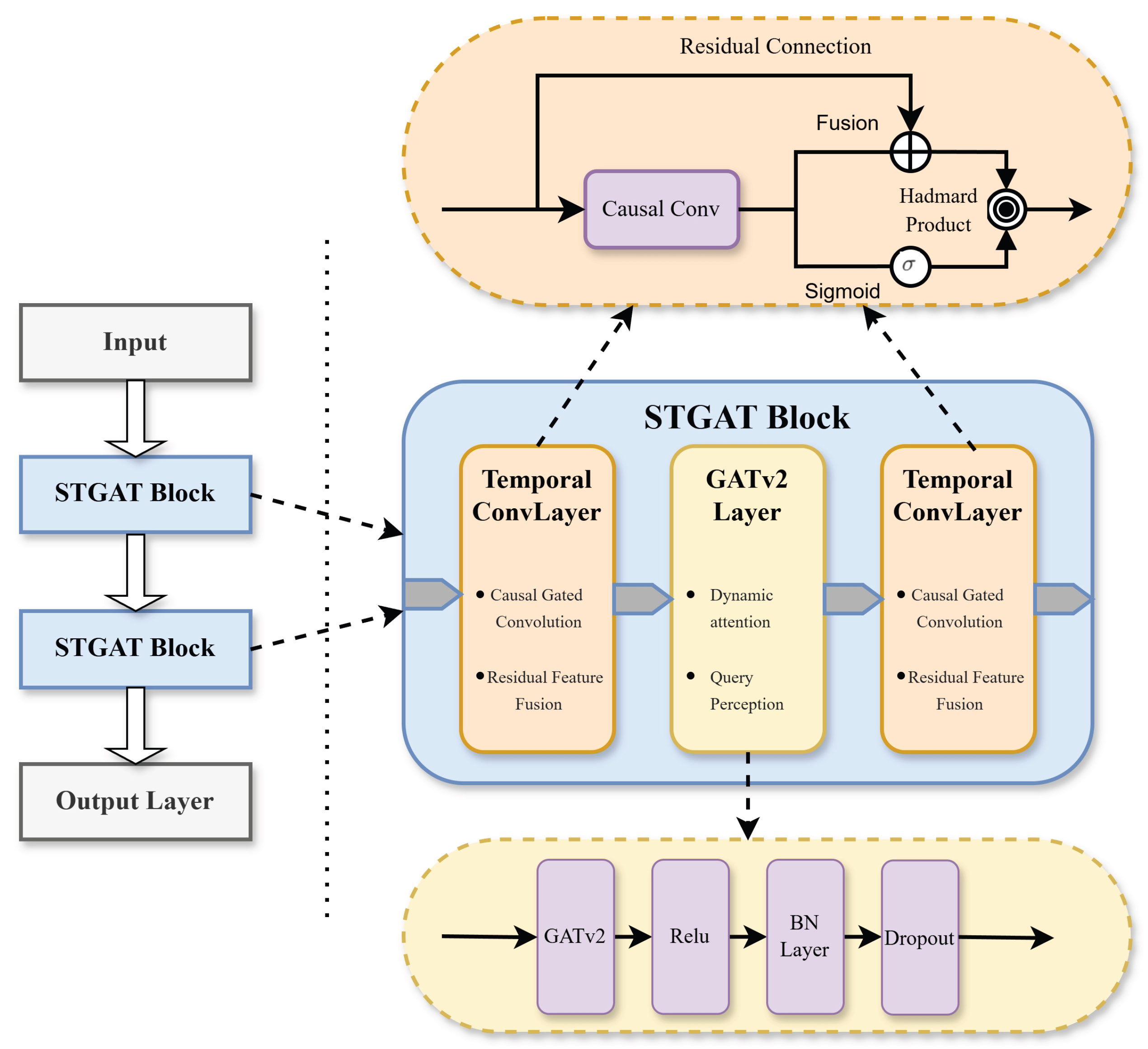
Figure 2.
This flowchart illustrates the STGAT pipeline for stock price prediction, integrating data preprocessing, model training, inference, and evaluation.
Figure 2.
This flowchart illustrates the STGAT pipeline for stock price prediction, integrating data preprocessing, model training, inference, and evaluation.
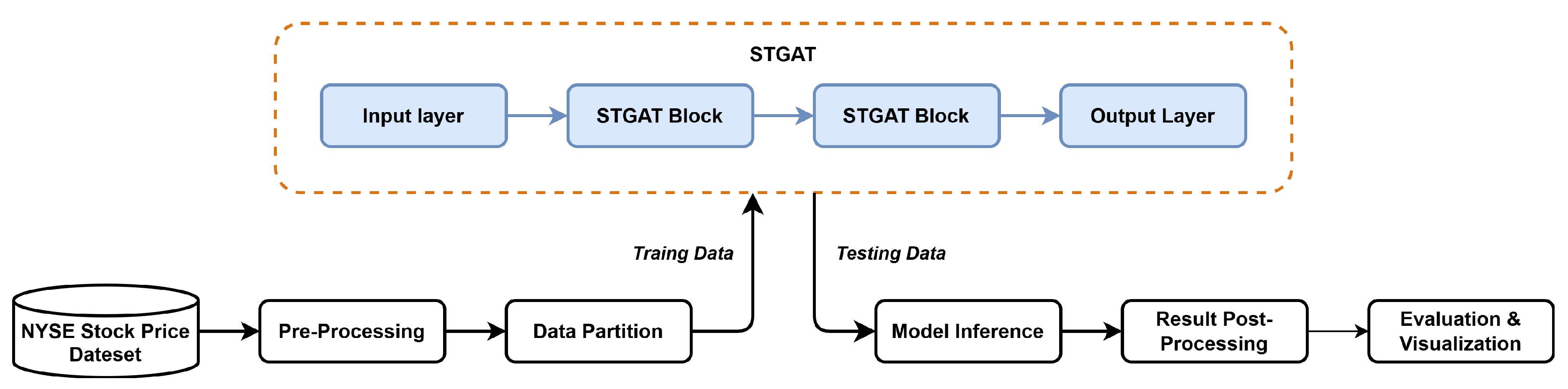
Figure 3.
RMSE values of fifteen stocks in commercial banks
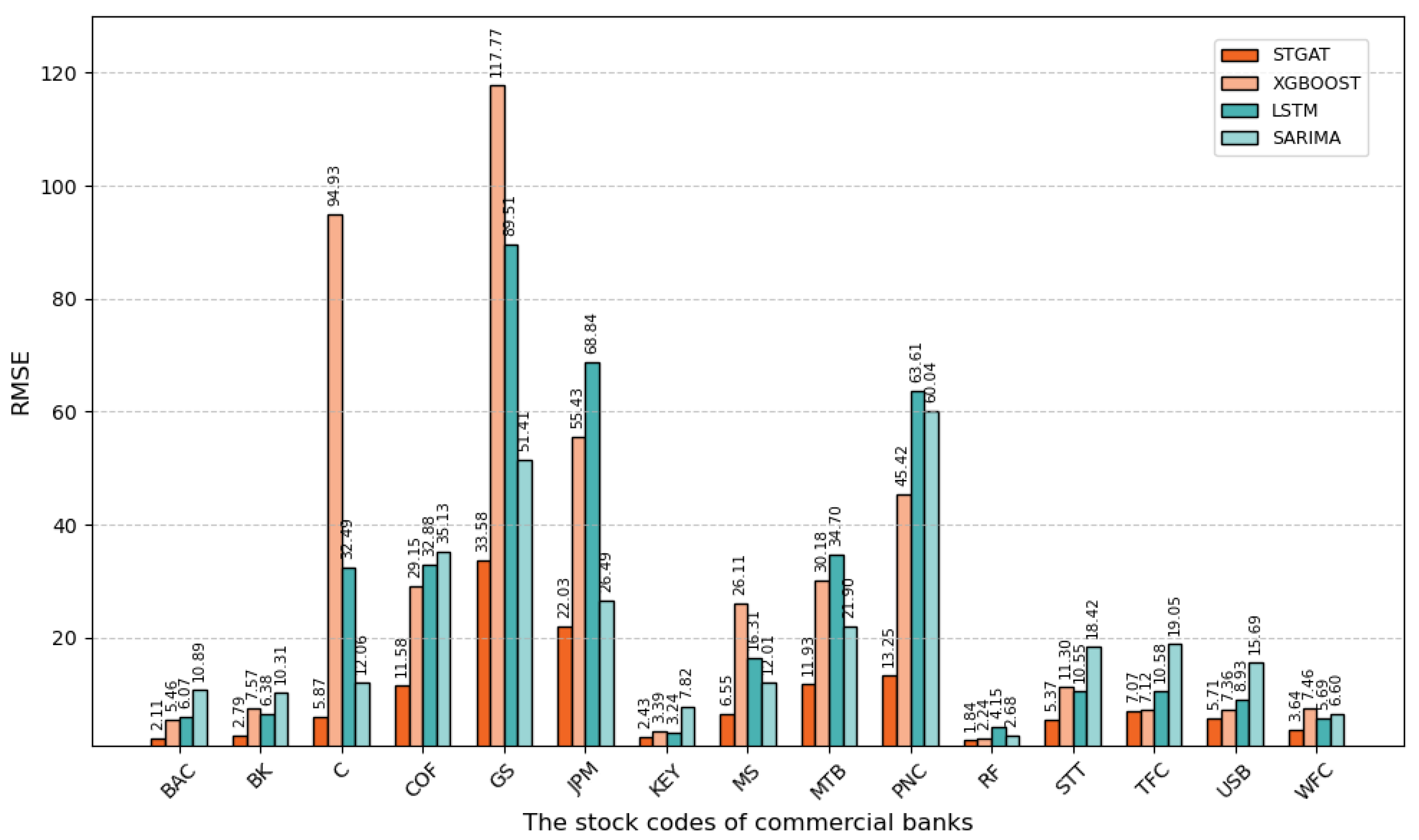
Figure 4.
MAE values of fifteen stocks in commercial banks
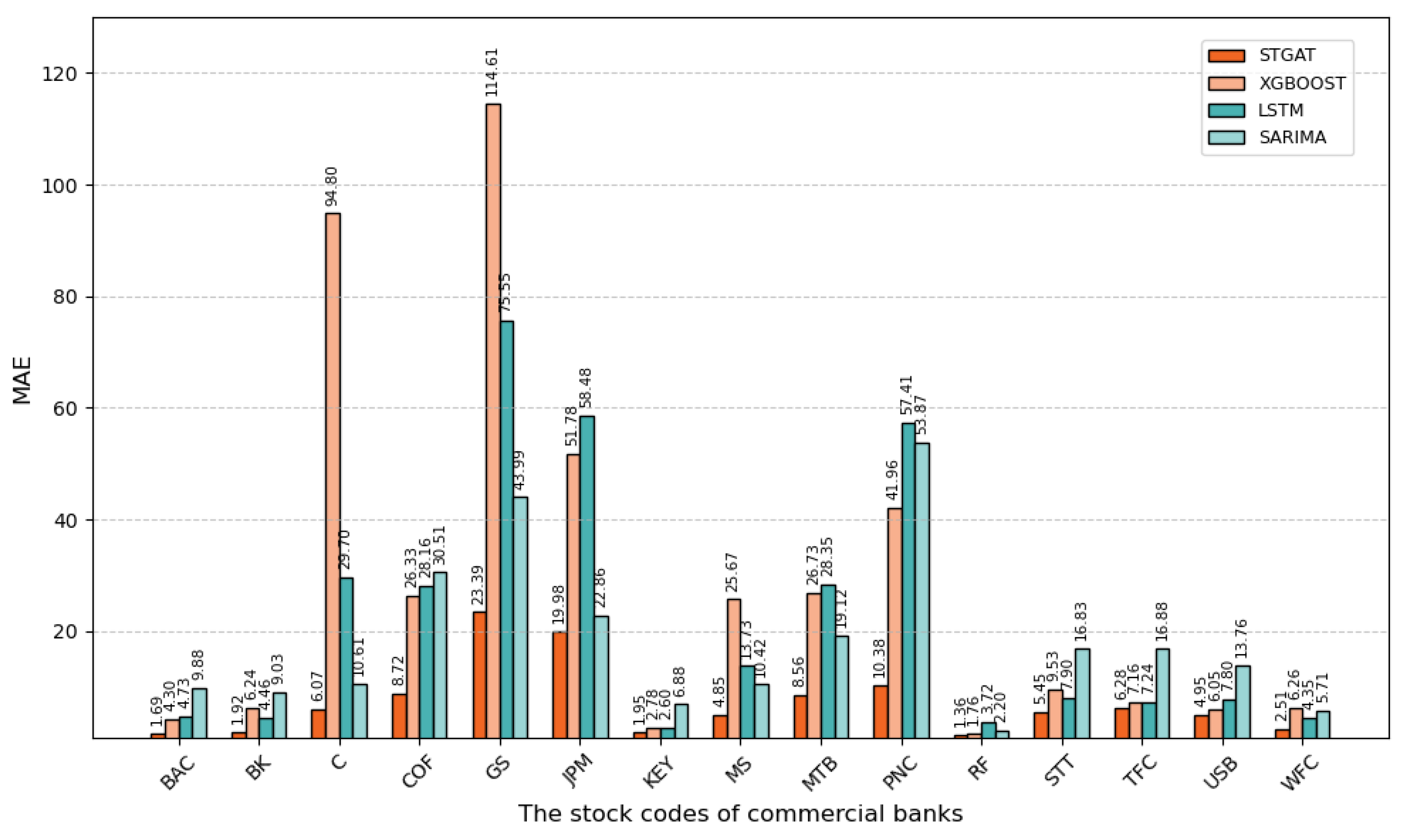
Figure 5.
Comparison of original and predicted values of KEY in commercial banks
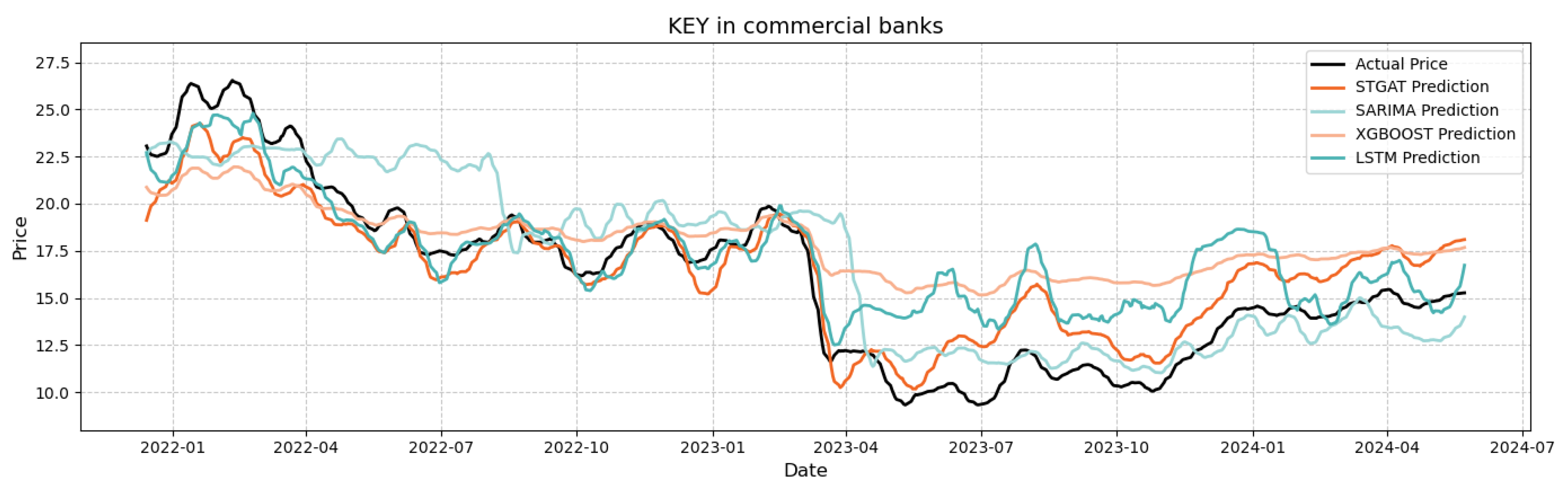
Figure 6.
Comparison of original and predicted values of RF in commercial banks
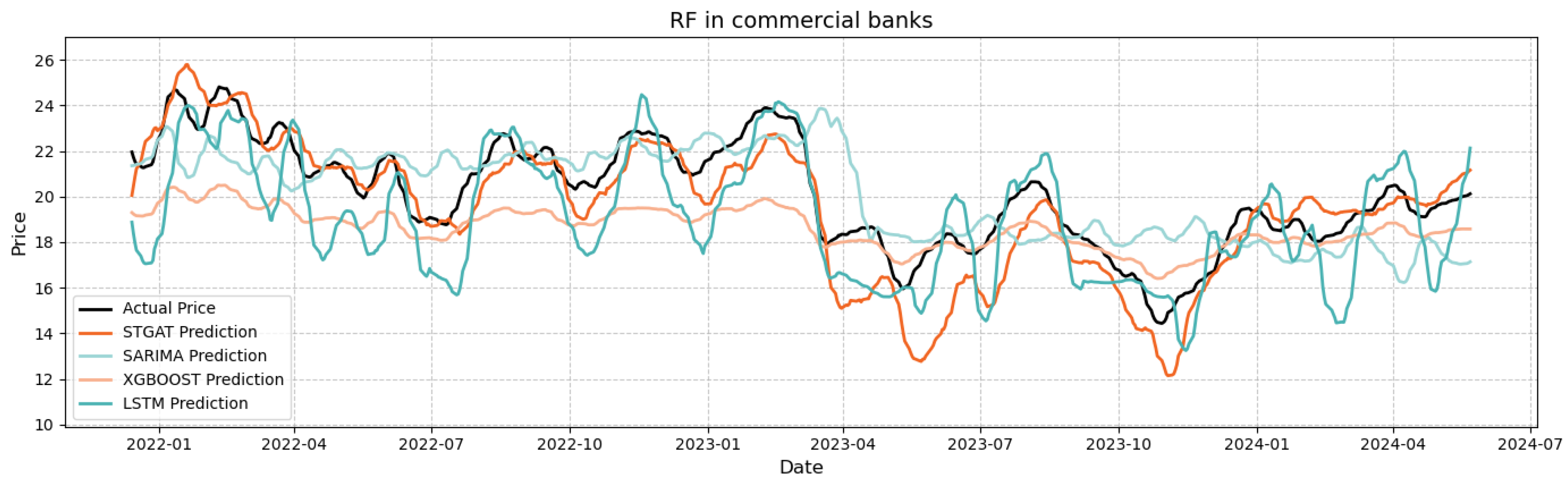
Figure 7.
RMSE values of six stocks in metal sector
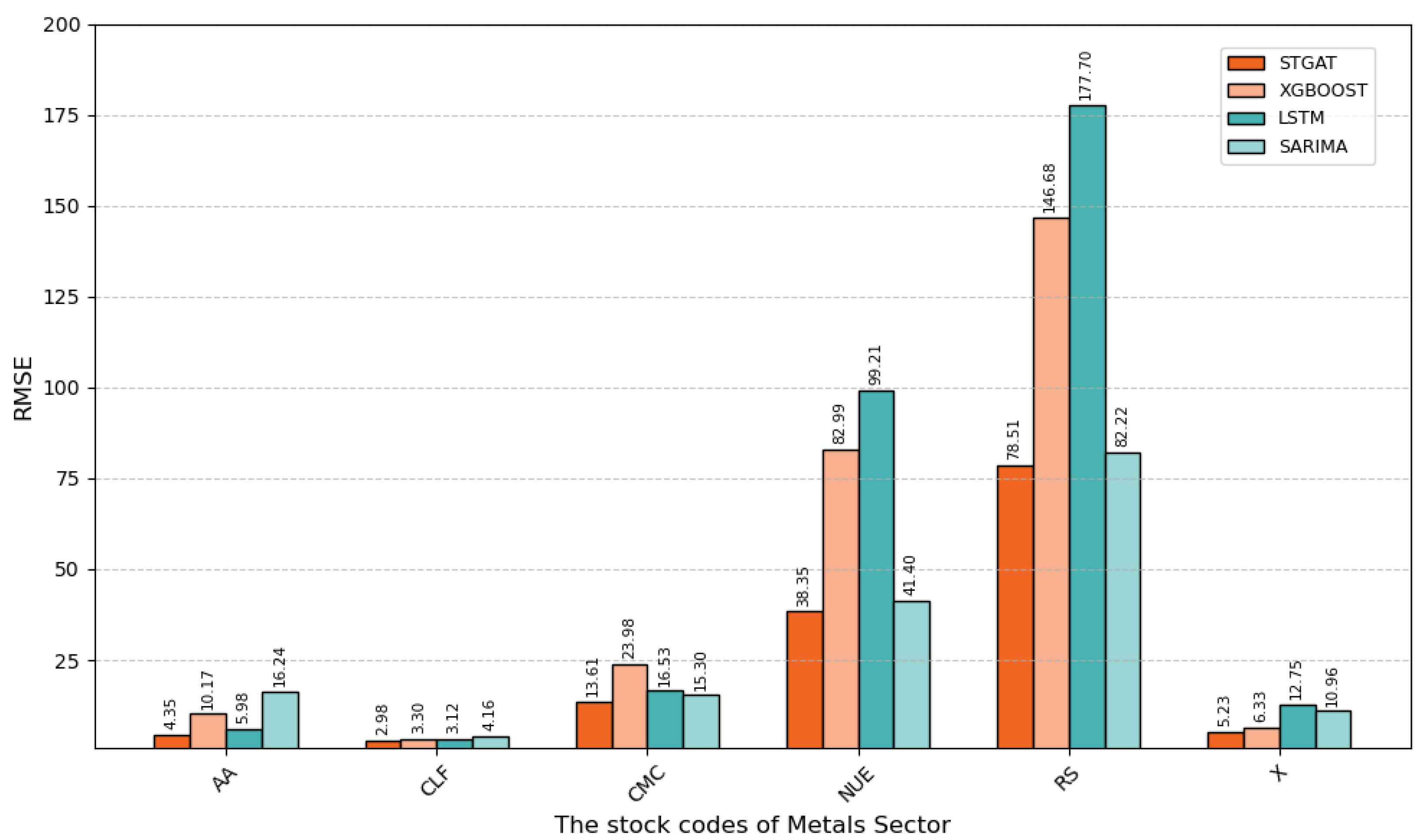
Figure 8.
MAE values of six stocks in metal sector
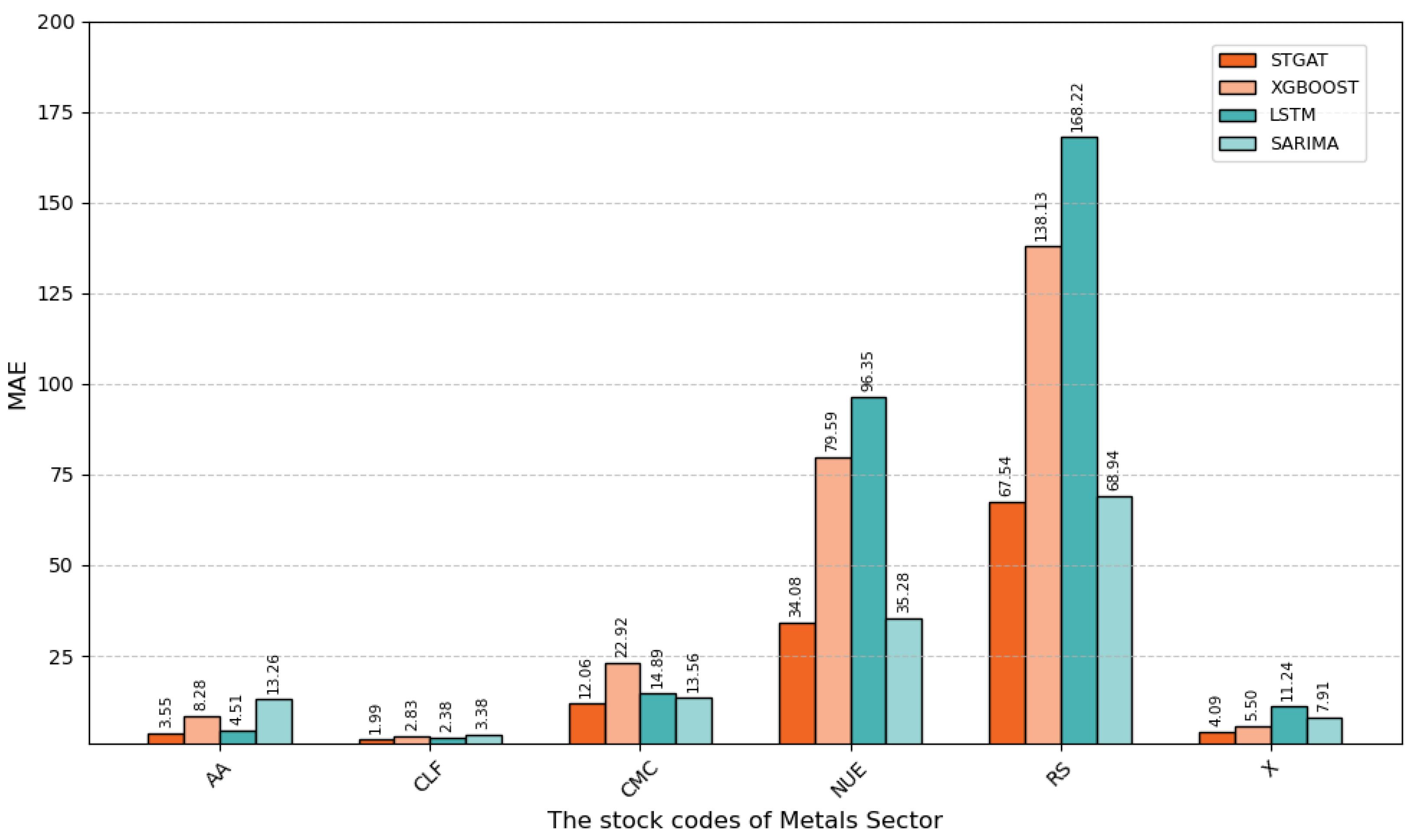
Figure 9.
Comparison of original and predicted values of AA in metal sector
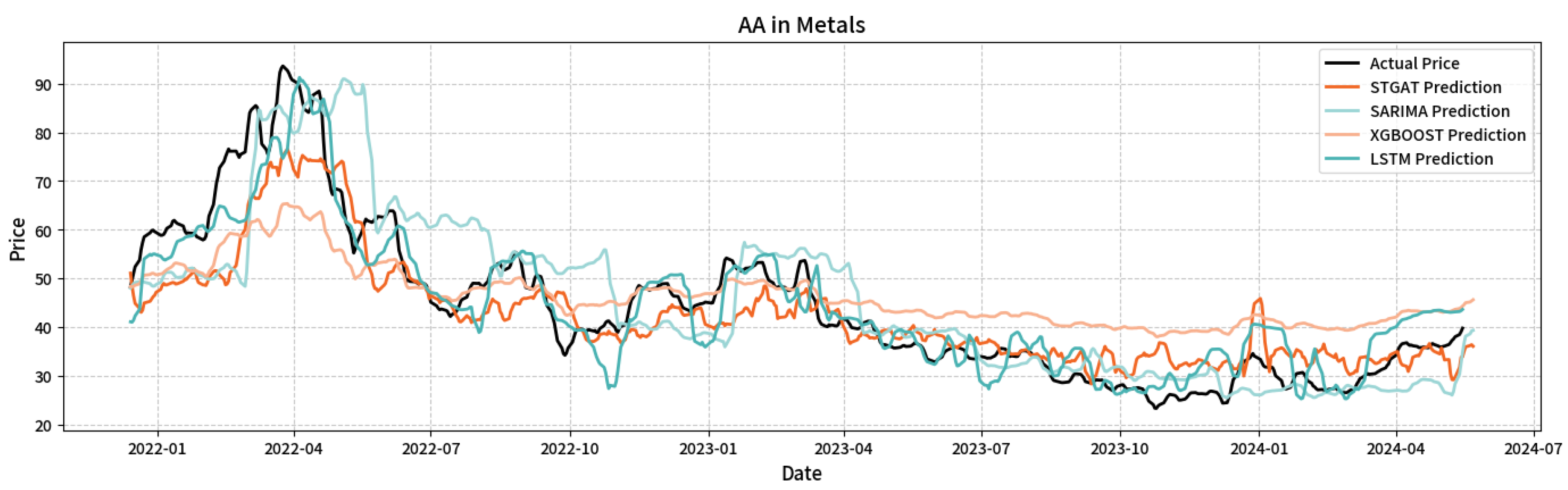
Figure 10.
Comparison of original and predicted values of CLF in metal sector
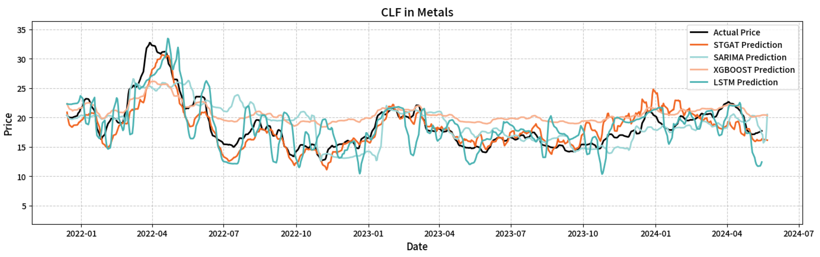
Figure 11.
Comparison of all ablated models in KEY and RF
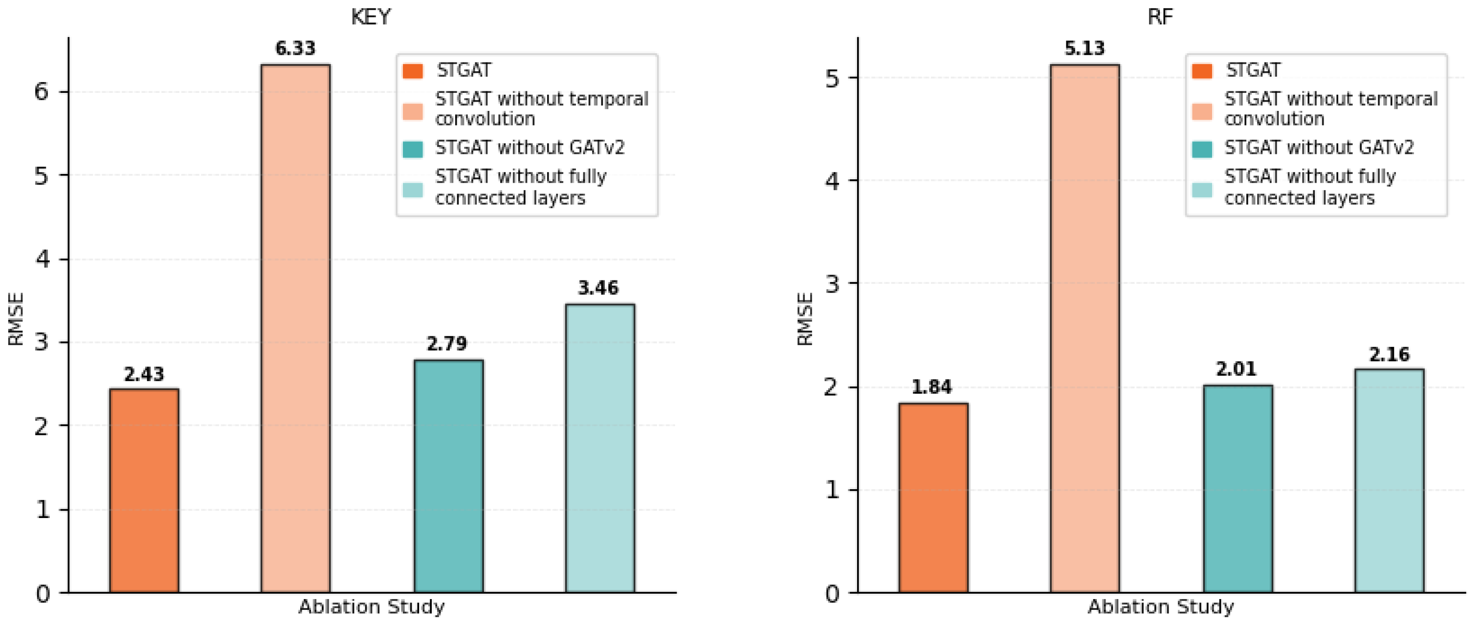
Figure 12.
Comparison of all ablated models in AA and CLF
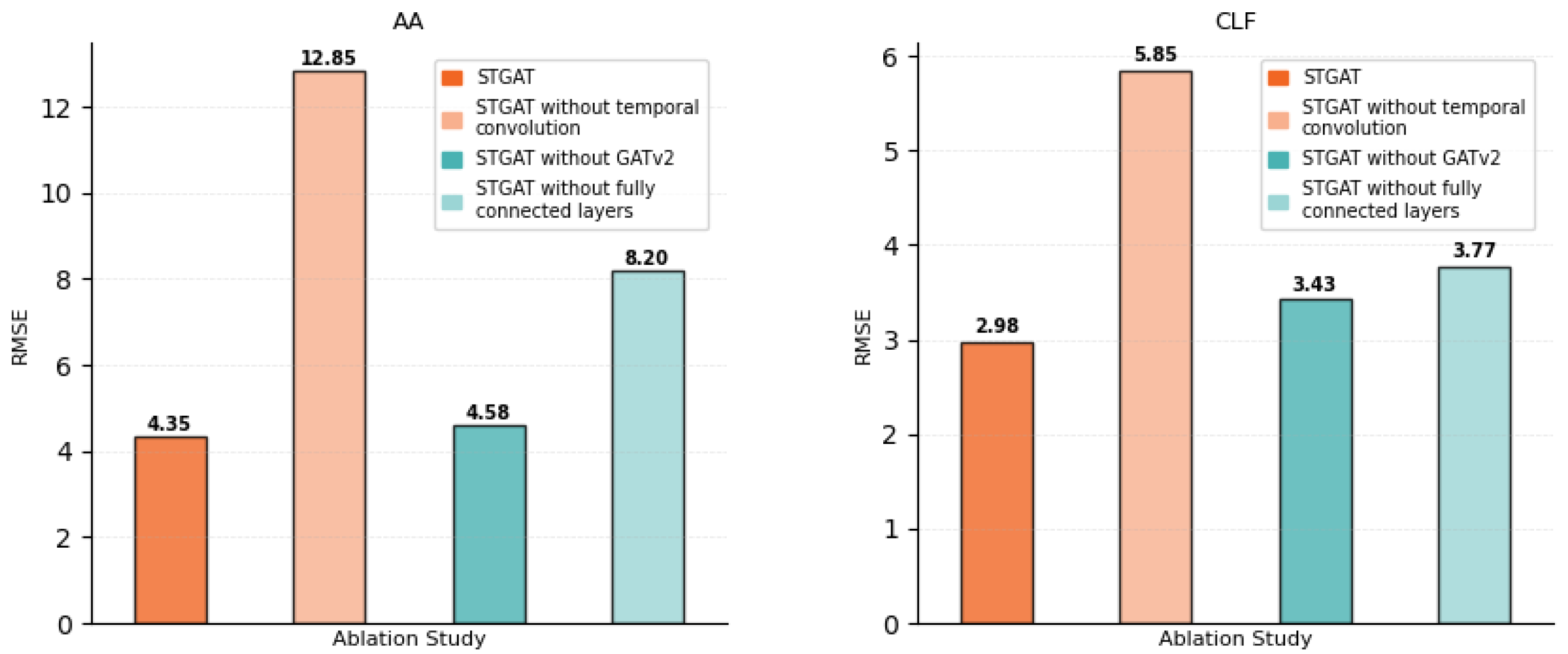

Table 1.
Training time in seconds.
| Model | Total time | Unit | |
|---|---|---|---|
| Commercial Bank Sector | Metals sector | ||
| STGAT | 1344 | 530 | seconds |
| XGBOOST | 1503 | 213 | seconds |
| LSTM | 397 | 180 | seconds |
| SARIMA | 813 | 231 | seconds |
Disclaimer/Publisher’s Note: The statements, opinions and data contained in all publications are solely those of the individual author(s) and contributor(s) and not of MDPI and/or the editor(s). MDPI and/or the editor(s) disclaim responsibility for any injury to people or property resulting from any ideas, methods, instructions or products referred to in the content. |
© 2025 by the authors. Licensee MDPI, Basel, Switzerland. This article is an open access article distributed under the terms and conditions of the Creative Commons Attribution (CC BY) license (http://creativecommons.org/licenses/by/4.0/).
Copyright: This open access article is published under a Creative Commons CC BY 4.0 license, which permit the free download, distribution, and reuse, provided that the author and preprint are cited in any reuse.


