
Submitted:
30 October 2025
Posted:
31 October 2025
You are already at the latest version
Abstract
Forecasting stock prices remains a central challenge in financial modelling, as markets are influenced by complex interactions between macroeconomic and microeconomic factors, firm-level fundamentals, and market sentiment. This study evaluates the predictive performance of classical statistical models and advanced attention-based deep learning architectures for daily stock price forecasting. Using a dataset of major U.S. equities and Exchange Traded Funds covering 2012–2024, we compare traditional statistical approaches, Seasonal Autoregressive Integrated Moving Average (SARIMA) and Exponential Smoothing, with deep learning architectures such as the Temporal Fusion Transformer (TFT), and the novel TFT-Graph Neural Network (TFT-GNN) hybrid that incorporates relational information between assets. All models are assessed under consistent experimental conditions in terms of forecast accuracy, computational efficiency, and interpretability. Results indicate that whilst statistical models offer strong baselines with high stability and low computational cost, the TFT outperforms them in capturing short-term nonlinear dependencies. The hybrid TFT-GNN achieves the highest overall predictive accuracy, demonstrating that relational signals derived from inter-asset connections provide meaningful enhancements beyond traditional temporal and technical indicators. These findings underscore the benefits of integrating relational learning into temporal forecasting frameworks and highlight the continued relevance of statistical models as interpretable, efficient benchmarks for evaluating deep learning approaches in high-frequency financial prediction.
Keywords:
stock price forecasting
; time series prediction
; statistical models
; Temporal Fusion Transformer (TFT)
; Graph Neural Networks (GNN)
; hybrid deep learning
; financial modelling
; attention mechanisms
1. Introduction
Stock price prediction is a major challenge for financial modelling due to market volatility and complexity. Despite advances in data availability and computation, developing models that consistently deliver accurate short-term forecasts remains difficult.
Classical statistical approaches such as Seasonal Autoregressive Integrated Moving Average (SARIMA) and Exponential Smoothing via the Error, Trend, Seasonal (ETS) framework offer strong and interpretable baselines with high computational efficiency. However, they often struggle to capture complex, dynamic, and nonlinear dependencies that deep learning models handle more effectively [1]. Recurrent architectures such as the Long Short-Term Memory (LSTM) models have therefore been widely applied to financial time series forecasting; see [2] for an introduction with Python, and [3] for an introduction to the MathWorks® Deep Learning Toolbox. Recent attention-based architectures, particularly the Temporal Fusion Transformer (TFT), have demonstrated superior performance in multivariate time series forecasting by combining recurrent and attention mechanisms [4].
This study evaluates and compares statistical models, the TFT, and a novel Temporal Fusion Transformer - Graph Neural Network (TFT-GNN) hybrid for daily stock price forecasting using a dataset of major U.S. equities and Exchange Traded Funds from 2012–2024.
The TFT-GNN model utilises relational data, which is often overlooked in stock market prediction; a survey by Jiang et al. [5] covering 124 stock prediction papers shows that only 4.2% used relational data. Most studies rely solely on historical prices or prices with technical indicators. This paper addresses that gap by integrating historical and relational data via GNNs, which remain largely unexplored in stock market forecasting, with many recent reviews omitting them entirely [6,7].
Results show that while statistical models remain competitive for stability and interpretability, the TFT-GNN achieves the highest predictive accuracy by incorporating relational information between assets. These findings highlight the benefits of integrating graph-based signals into temporal forecasting frameworks and provide practical insights into balancing predictive performance and interpretability in financial modelling.
2. Methodology
2.1. Overview
This study adopts a comparative modelling approach to evaluate statistical and deep learning methods for daily stock price forecasting. Specifically, two statistical baselines: SARIMA and Exponential Smoothing via ETS, are compared with two attention-based architectures: the TFT and TFT-GNN hybrid. All models were implemented under consistent data, training, and evaluation settings to ensure a fair comparison.
2.2. Data and Preprocessing
Daily OHLCV (open, high, low, close, volume) data for Apple (AAPL), JPMorgan Chase (JPM), NVIDIA (NVDA), and the S&P 500 Exchange-Traded Fund (ETF) (SPY) were obtained using the Yahoo Finance API via the yfinance Python module, covering 2012-2024.
In addition to the four primary stocks/ETFs, the full set of NASDAQ-traded securities was retrieved, with ticker symbols obtained from the NASDAQ Trader symbol directory [8]. These additional securities were essential for constructing the relational data required by the hybrid TFT-GNN model.
While the statistical models were univariate, using only closing prices, the deep learning models required extensive feature engineering, using OHLCV data to generate lagged variables and technical indicators. Feature selection was performed both before and after training. Highly correlated feature pairs were reduced to avoid redundancy, while weak linear correlation with the target did not preclude inclusion, as nonlinear, time-dependent patterns may still hold predictive value. Figure 1 shows the correlation heatmap of engineered and raw variables for AAPL, used to identify highly correlated features.
2.3. Problem Framing and Experimental Setup
The forecasting task was framed as a regression problem targeting the daily closing price. Three temporal splits were used to ensure robustness:
- Training & validation 2012–2017, test 2018.
- Training & validation 2015–2020, test 2021.
- Training & validation 2018–2023, test 2024.
A rolling-window validation procedure was applied for hyperparameter tuning, and models were retrained on full training data before evaluation on the holdout year.
2.4. Models
2.4.1. Statistical Models
SARIMA, introduced by Box et al. in 1970 [9], comprises four components: autoregressive (dependence on past values, p), integrated (differencing to ensure stationarity, d), moving average (lagged error terms, q), and are their seasonal counterparts, with period s. A full grid search of all 7 hyperparameters was computationally infeasible, so the parameter space was constrained:
- , , .
- , , .
Exponential Smoothing, introduced by Robert G. Brown in 1956 [10] and further developed in his 1959 book [11], forecasts future values by assigning exponentially decreasing weights to past observations. Its simplicity and effectiveness in short-term forecasting contributed to its popularity [12]. In 2002, Rob J. Hyndman extended this approach by introducing the ETS framework [13], which explicitly models the components of forecasting errors, trends, and seasonality in additive or multiplicative forms, with seasonal periods of 5, 21, and 63 days considered.
2.4.2. Deep Learning Models
The TFT was implemented using the PyTorch Forecasting library, combining variable selection networks, gated residual blocks, and interpretable attention layers. Originally introduced by Lim et al. at Google Research in 2021 [14], the TFT is a transformer-based architecture designed specifically for multi-horizon time-series forecasting. It builds upon the transformer framework first established in the seminal work “Attention Is All You Need” by Vaswani et al. [15], which introduced the self-attention mechanism that allows models to efficiently capture long-term dependencies in sequential data.
Unlike standard recurrent or convolutional approaches, the TFT explicitly separates static, known, and observed time-varying inputs through dedicated encoders, allowing it to model both temporal dynamics and static metadata simultaneously. The model architecture consists of a sequence of gated residual networks (GRNs) for feature processing and variable selection networks (VSNs) that dynamically choose the most relevant covariates at each timestep. Temporal dependencies are modelled through a sequence-to-sequence LSTM backbone combined with multi-head self-attention, enabling the model to focus selectively on informative past time steps.
One of the key innovations of the TFT is its interpretable attention layer, which provides insight into which historical inputs most influenced the model’s forecasts. Although computationally intensive, the TFT’s hybrid design of attention and gating mechanisms achieves a balance between model expressiveness and interpretability, making it well-suited for high-dimensional financial time-series data.
Graph Neural Networks (GNNs), first proposed by Scarselli et al. [16], extend neural network operations to graph-structured data by iteratively aggregating information from neighboring nodes, enabling the model to capture relational dependencies. In financial contexts, this allows stocks to be represented as nodes linked by correlations, sector relationships, or supply-chain ties [17]. Graph Attention Networks (GATs), introduced by Veličković et al. [18], apply attention mechanisms to graph learning, allowing the network to assign adaptive importance weights to neighboring nodes. These architectures enable the modelling of both the structure and strength of inter-stock relationships, which is valuable in stock market prediction [19].
The TFT-GNN hybrid extended this framework by incorporating relational information from a GAT into the TFT’s temporal input layer. The GAT outputs were transformed into a simplified directional signal (up or down), allowing the TFT to leverage relational trends without excessive dimensional complexity. This integration enabled joint temporal-relational learning, improving predictive accuracy and interpretability compared to standalone temporal or graph-based models.
While both TFTs and GNNs have been applied to stock market prediction [20,21], the combination of the two as a hybrid model marks a novel contribution. In-depth details of the TFT and TFT-GNN’s hyperparameters are in Appendix A.1 and Appendix A.2, respectively.
2.5. Evaluation Metrics
Performance was assessed using Root Mean Squared Error (RMSE), Mean Absolute Error (MAE), Mean Absolute Percentage Error (MAPE), and Coefficient of Determination (R²). Together, these metrics capture error magnitude, scale-independent accuracy, and explanatory power. Model interpretability was further examined using attention weight visualisations for the TFT and TFT-GNN.
2.6. Implementation
All experiments were implemented in Python using Pandas, statsmodels, PyTorch, and PyTorch Forecasting. Training was conducted on Google Colab with GPU acceleration for the deep learning models. Code and data preprocessing scripts are available in Appendix B.
3. Results
3.1. Overview
This section presents the empirical results for the four selected models.. All experiments focus on daily stock price forecasting, evaluated on major U.S. equities and ETFs from 2018–2024. Models were compared using consistent datasets and metrics, with performance assessed in terms of predictive accuracy, computational efficiency, and interpretability.
Due to computational constraints, SARIMA was implemented using a weekly sliding-window approach, where each model was refit weekly and used to generate daily predictions for the subsequent week. In contrast, ETS, TFT, and TFT-GNN employed a daily rolling-window framework, updating the model each trading day using the most recent data.
3.2. Statistical Models
3.2.1. SARIMA
The SARIMA model produced mixed results across assets and time periods. While it captured recurring seasonal and autoregressive patterns, its linear formulation limited responsiveness to abrupt market shifts. Across all test periods, SARIMA achieved an average and . Performance across each stock was similar, despite the varying levels of volatility. Figure 2 shows the SARIMA model’s prediction for SPY in 2024.
Hyperparameter optimisation required significant computational time, and full daily retraining proved infeasible. Each forecast required approximately 1-2 minutes per stock, leading to total runtimes several times higher than ETS. Consequently, SARIMA was evaluated only under the weekly sliding-window scheme, which, while providing reasonable accuracy, limited its capacity for rapid adaptation to evolving market conditions.
3.2.2. Exponential Smoothing via ETS
The ETS model achieved strong predictive accuracy at a fraction of the computational cost of SARIMA. Its exponential updating mechanism enabled rapid adaptation to recent price dynamics, and daily retraining was computationally feasible.
Across assets, ETS achieved an average and , outperforming SARIMA in most daily settings. The model performed particularly well for volatile assets such as JPM and NVDA, as shown in Figure 3, where adaptive trend and seasonality components effectively captured short-term reversals.
Computation times averaged under five minutes per stock per year, making ETS the only statistical model suited to true daily rolling-window forecasting. While interpretability remained high, ETS occasionally lagged during sharp regime changes due to its assumption of locally smooth trends.
3.3. Deep Learning Models
3.3.1. TFT
The TFT achieved superior predictive performance compared with the statistical baselines while maintaining manageable training times. The architecture effectively captured nonlinear temporal dependencies and provided interpretable feature importance and attention weight visualisations. On average, the model achieved and , representing an improvement over ETS. Figure 4 shows one of the TFT’s strongest predictions: SPY in 2021.
Feature attribution (Figure 5(a)) indicated that the Relative Strength Index (RSI) and Moving Average Convergence Divergence (MACD) were the most influential technical indicators, while trading volume contributed minimally. Temporal attention plots (Figure 5(b)) showed that the model focused primarily on the most recent 5–10 trading days, consistent with short-term market memory. Training each period required approximately 5 minutes, confirming the model’s practicality for daily rolling forecasts.
3.3.2. Hybrid TFT - GNN
Integrating graph-based relational information further improved predictive accuracy. The TFT-GNN hybrid achieved the best overall results, with an average and , outperforming the standalone TFT in 11 of 12 evaluated periods. The hybrid’s strongest performance occurred for SPY in 2024, shown in Figure 6 where it achieved , the highest of all models.
Using a simplified GNN-derived up/down signal produced superior results to high-dimensional graph embeddings, suggesting that compact relational cues are more informative for daily prediction tasks.
Attention analysis revealed that graph-derived relational signals were assigned greater weight than conventional indicators such as RSI and MACD, shown in Figure 7.
Training times averaged minutes per period, around double the TFT baseline, confirming that superior predictive performance comes at a higher computational cost.
3.4. Comparative Summary
ETS was the strongest statistical model, balancing accuracy, interpretability, and computational efficiency. The TFT-GNN achieved the highest overall predictive accuracy, demonstrating the value of combining temporal attention with relational graph information. Comprehensive results are in Appendix C, and the findings are summarised in Table 1.
Overall, the results indicate that while traditional statistical models remain competitive baselines, attention-based architectures, and particularly the TFT-GNN hybrid, offer significant improvements in predictive accuracy without prohibitive computational cost. The findings highlight the practical benefits of integrating relational information into temporal forecasting models for daily financial prediction.
4. Discussion
The comparative evaluation reveals distinct trade-offs between predictive accuracy, computational feasibility, and interpretability across the model families examined. Although deep learning models often dominate in complex sequence modelling, the results here reaffirm the continued competitiveness of statistical methods for financial time series forecasting when appropriately tuned and constrained.
4.1. Statistical Models
The statistical models exhibited consistent and interpretable behaviour, with performance differences largely explained by each model’s capacity to handle volatility and adapt to evolving patterns. Due to computational constraints, SARIMA was trained using a weekly sliding-window approach, which iteratively generated daily forecasts rather than retraining each day as in the daily rolling-window setup used for other models. This compromise allowed fair comparison across methods while maintaining computational tractability.
Among the statistical approaches, ETS achieved the strongest results under the daily rolling-window regime. Its adaptive smoothing mechanisms provided effective short-horizon responsiveness with minimal training overhead. SARIMA achieved comparable accuracy under the weekly window, with optimal parameters frequently close to , aligning with previous findings in financial forecasting literature [22].
Overall, ETS proved the most practical for daily deployment, while SARIMA demonstrated value in longer-horizon or lower-frequency contexts where retraining costs are less prohibitive. These findings reinforce prior conclusions that classical statistical models remain strong baselines for short-term market forecasting, particularly when interpretability and efficiency are prioritised over incremental accuracy gains.
4.2. TFT
The TFT outperformed the statistical baselines on the daily forecasting horizon. Its ability to selectively attend to recent observations and key covariates enabled the model to capture short-term dependencies more effectively than fixed-structure statistical methods. Attention-based interpretability further revealed that the most influential features were short-term momentum and volatility indicators, while volume contributed minimally, consistent with established findings in stock market prediction research.
Despite its greater complexity, the TFT trained efficiently on GPU, with convergence stability and reproducibility that contrasted other deep learning model’s, such as LSTMs, known difficulties under long sequences [23]. The TFT therefore represents a practical balance between model expressiveness and operational feasibility for daily financial forecasting tasks.
4.3. TFT-GNN Hybrid
The hybrid TFT-GNN model delivered the highest predictive accuracy of all tested approaches. By incorporating graph-derived relational signals into the TFT architecture, the model was able to account for inter-stock dependencies, capturing latent market structure that is otherwise invisible to univariate or purely temporal models.
Attention analysis revealed that the TFT component consistently assigned greater weight to the GNN-derived relational features than to traditional technical indicators such as RSI and MACD, suggesting that inter-asset relationships provide a richer and more predictive representation of market dynamics. These findings align with emerging research demonstrating that graph-based financial models can extract sectoral and co-movement structures that meaningfully enhance temporal forecasting performance.
From an applied perspective, the TFT-GNN strikes a favourable balance between accuracy, interpretability, and computational cost. While its training demands are higher than those of ETS or SARIMA, the hybrid’s superior accuracy and transparency through attention mechanisms make it a compelling candidate for near-term, production-level financial forecasting systems.
4.4. Summary
In summary, the comparative analysis underscores the nuanced trade-offs between traditional and neural forecasting paradigms. ETS remains an efficient and interpretable baseline, TFT provides substantial accuracy improvements with manageable computational cost, and the TFT-GNN extends this further by integrating relational structure into temporal modelling. The results collectively highlight the value of incorporating graph-based relational information into transformer-based frameworks for stock price forecasting, offering both empirical accuracy gains and deeper interpretive insight into market dependencies.
5. Conclusions
This study evaluated the performance of statistical and deep learning approaches for daily stock price forecasting, focusing on SARIMA, ETS, TFT, and a hybrid TFT-GNN model. Among the statistical methods, ETS proved most effective under the daily rolling-window framework due to its low computational cost and adaptive smoothing, while SARIMA remained valuable for longer-horizon or weekly sliding-window forecasts despite their higher computational demands. These results reaffirm the continued relevance of classical statistical models as robust and interpretable baselines.
The TFT demonstrated clear advantages over standalone statistical methods, capturing short-term temporal dependencies and providing interpretable feature attributions. Incorporating relational information via the TFT-GNN hybrid further improved predictive accuracy, with attention analysis indicating that graph-derived signals contributed more strongly than conventional technical indicators. This highlights the importance of integrating inter-asset relationships into temporal forecasting models.
Beyond financial forecasting, the proposed framework could be adapted to other time-series domains, where relational dependencies and temporal dynamics play equally important roles, such as energy demand [24], traffic congestion [25], or healthcare analytics [26]. In practical financial contexts, this approach could support tasks such as portfolio optimisation and risk assessment by providing interpretable and data-driven forecasts tailored to specific market conditions.
Hybrid approaches are proving ever popular, recent publications include: a novel integrate the first moment (mean) and second-moment (variance) components of stock price dynamics to forecast future price trends [27]; an integrated Convolutional Neural Network (CNN)-attention mechanism-LSTM model to enhance the prediction of temporal patterns in financial time series [28]; and a combined Adaptive Gaussian Short-Term Fourier Transform (AG-STFT) and Mamba framework model for stock price prediction [29], for example.
Overall, the findings demonstrate that hybrid architectures combining temporal learning and relational reasoning offer the best balance of accuracy, interpretability, and computational feasibility for daily stock price prediction. Future work could explore dynamic or multi-layered graph structures, probabilistic forecasting, and applications to broader asset classes, extending the practical utility of hybrid transformer-graph models in financial forecasting.
Author Contributions
All authors have read and agreed to the published version of the manuscript.
Funding
This research received no external funding.
Data Availability Statement
The original contributions presented in the study are included in the article; further inquiries can be directed to the corresponding author.
Acknowledgments
The authors thank the anonymous referees for their valuable comments and suggestions that led to the improvement of this paper.
Conflicts of Interest
The authors declare no conflicts of interest.
Abbreviations
The following abbreviations are used in this manuscript:
| AAPL | Apple Inc. |
| AG-STFT | Adaptive Gaussian Short-Term Fourier Transform |
| CNN | Convolutional Neural Network |
| ETS | Exponential Smoothing (Error, Trend, Seasonal) Model |
| ETF | Exchange-Traded Fund |
| GAT | Graph Attention Network |
| JPM | JPMorgan Chase & Co. |
| MACD | Moving Average Convergence Divergence |
| NVDA | NVIDIA Corporation |
| OHLCV | Open, High, Low, Close, Volume |
| Coefficient of Determination | |
| RMSE | Root Mean Squared Error |
| RSI | Relative Strength Index |
| SARIMA | Seasonal Autoregressive Integrated Moving Average |
| SPY | SPDR S&P 500 ETF Trust |
| TFT | Temporal Fusion Transformer |
| TFT-GNN | Temporal Fusion Transformer with Graph Neural Network integration |
Appendix A. Hyperparameter Tuning
Appendix A.1. TFT Model
The TFT shares several hyperparameters with standard recurrent architectures, including dropout rate, learning rate, number of epochs, early stopping, batch size, loss function, optimizer, lookback window size, input features, and prediction horizon. Key TFT-specific hyperparameters are as follows:
- Encoder and Decoder Layers: Number of stacked LSTM layers in the encoder and decoder modules. Deeper layers increase model capacity but risk overfitting.
- Hidden Layer Size: Dimensionality of the model’s internal layers, influencing its representational capacity.
- Attention Heads: Number of parallel attention mechanisms in the multi-head attention block; additional heads capture diverse patterns at higher computational cost.
- Static Embedding Size: Dimensionality of learned embeddings for static covariates.
- Time-Varying Embedding Size: Dimensionality of learned embeddings for time-varying features such as lagged prices or technical indicators.
- Variable Selection: Boolean flag indicating whether to use input variable selection networks for dynamic feature relevance estimation.
- Attention Window: Number of past time steps accessible to the temporal attention mechanism.
Initial configurations used Close and Volume as input variables, with a learning rate of , hidden size of 128, attention head size of 2, dropout rate of , batch size of 64, attention window size of 30, and SMAPE loss.
Empirical testing indicated that a lookback window of 30 days yielded the best results, with both shorter and longer windows reducing accuracy. Reducing the hidden size from 128 to 64 improved generalization. Increasing dropout to or reducing batch size to 32 degraded performance. Varying attention heads confirmed that two heads were optimal, as one or three performed worse. Final configurations balanced interpretability and computational efficiency, providing consistent daily rolling-window performance across assets.
Appendix A.2. TFT-GNN Model
The GNN and subsequent TFT–GNN hybrid were trained using a diverse universe of U.S. equities and sector ETFs to capture inter-asset relationships. These were grouped as follows:
- Apple Supply Chain and Related: AAPL, AMD, TSM, AVGO, ASML, QCOM, TXN, MU, NXPI, KLAC, LRCX, ADI, AMAT, MCHP
- Big Tech Peers: GOOGL, MSFT, AMZN, META, NFLX, ORCL, SONY, CRM, ADBE
- Financials: JPM, MS, BAC, BLK, GS, WFC, SCHW, BK, AXP, COF, MET
- Semiconductors: NVDA, AMD, TSM, ASML, QCOM, MU, TXN, NXPI, KLAC, LRCX
- Healthcare: UNH, JNJ, PFE, MRK, LLY, TMO, BMY, NVO
- Automotive: TSLA, F, GM, HMC, TM
- Consumer: WMT, HD, COST, PG, KO, MCD, TGT, PEP
- Exchange-Traded Funds (ETFs): SPY, QQQ, DIA, IWM, XLK, XLF, XLE, XLI, XLV, XLY, XLP, VNQ, IYR, VGT, VTI, VUG, VTV, IWF, IWD, ITOT
The GNN was implemented as a Graph Attention Network (GAT) with tunable parameters including:
- Node Features: Input features for each stock (e.g., OHLCV, RSI, MACD).
- Hidden Channels: Dimensionality of intermediate node embeddings.
- Number of GAT Layers: Controls network depth; deeper models capture higher-order relations but risk over-smoothing.
- Attention Heads: Number of attention mechanisms applied per layer.
- Dropout Rate, Learning Rate, and Optimizer: Standard training hyperparameters.
The TFT-GNN hybrid extended the base TFT by incorporating relational information from the Graph Neural Network (GNN). Initial experiments injected raw 128-dimensional GNN embeddings directly into the TFT input, but this degraded performance due to excessive dimensionality.
To address this, a multilayer perceptron (MLP) was introduced to progressively reduce embedding dimensionality. Reductions from were tested, with smaller embeddings yielding improved stability though performance remained near the TFT baseline.
Subsequently, GNN embeddings were transformed into a simplified up/down signal, representing directional market tendencies. Incorporating this signal produced a measurable improvement in predictive accuracy and interpretability. Additional tuning revealed that employing a lower learning rate and retaining an attention head size of 2 further stabilized training and improved consistency across different assets.
Appendix B. Code Repository
An example code for each model can be found at this GitHub link:
In addition, a complete archive of all notebooks used in the making of this article has been uploaded to the same repository to ensure full reproducibility.
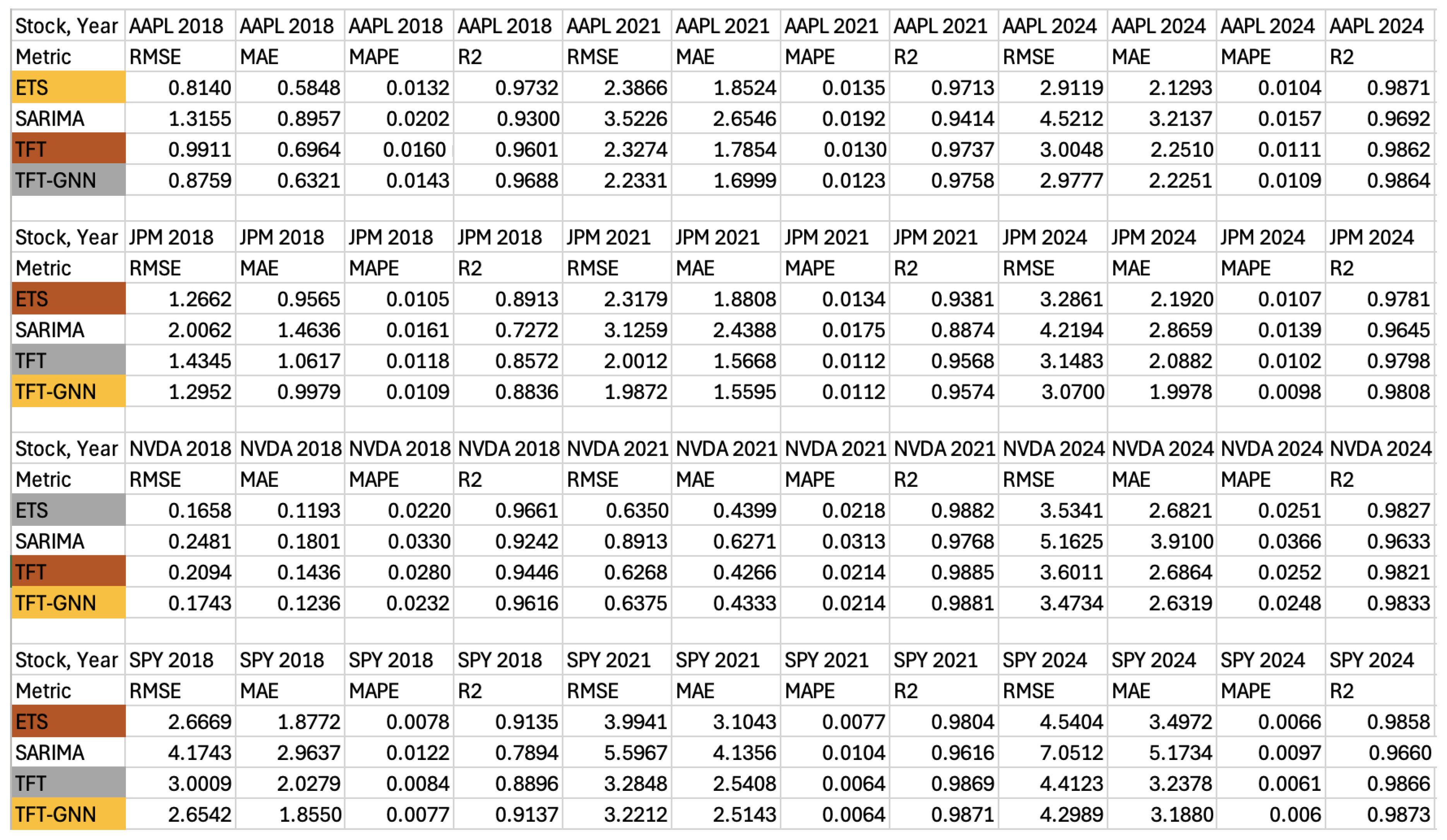
Appendix C. Table of Results
Figure A1 shows the performance metrics for each model, across each time period and security.
Figure A1.
Comprehensive results for each model.
References
- Lara-Benítez, P.; Carranza-García, M.; Riquelme, J.C. An experimental review on deep learning architectures for time series forecasting. International journal of neural systems 2021, 31, 2130001. [Google Scholar] [CrossRef]
- Lynch, S. Python for Scientific Computing and Artificial Intelligence; Chapman and Hall/CRC, 2023. [Google Scholar]
- Lynch, S. Dynamical Systems with Applications using MATLAB, 3rd ed.; Springer Nature, 2025. [Google Scholar]
- Olorunnimbe, K.; Viktor, H. Ensemble of temporal Transformers for financial time series. Journal of Intelligent Information Systems 2024, 62, 1087–1111. [Google Scholar] [CrossRef]
- Jiang, W. Applications of deep learning in stock market prediction: recent progress. Expert Systems with Applications 2021, 184, 115537. [Google Scholar] [CrossRef]
- Ajiga, D.I.; Adeleye, R.A.; Tubokirifuruar, T.S.; Bello, B.G.; Ndubuisi, N.L.; Asuzu, O.F.; Owolabi, O.R. Machine learning for stock market forecasting: a review of models and accuracy. Finance & Accounting Research Journal 2024, 6, 112–124. [Google Scholar] [CrossRef]
- Kehinde, T.; Chan, F.T.; Chung, S.H. Scientometric review and analysis of recent approaches to stock market forecasting: Two decades survey. Expert Systems with Applications 2023, 213, 119299. [Google Scholar] [CrossRef]
- NASDAQ. Nasdaqtraded.txt – NASDAQ Symbol Directory. https://www.nasdaqtrader.com/dynamic/SymDir/nasdaqtraded.txt. Accessed: 23/04/2025.
- Box, G.E.; Jenkins, G.M.; Reinsel, G.C.; Ljung, G.M. Time series analysis: forecasting and control; John Wiley & Sons, 2015. [Google Scholar]
- Brown, R.G. Exponential smoothing for predicting demand; Little, 1956. [Google Scholar]
- Brown, R. Statistical Forecasting for Inventory Control; McGraw-Hill, 1959. [Google Scholar]
- Gardner Jr, E.S. Exponential smoothing: The state of the art. Journal of forecasting 1985, 4, 1–28. [Google Scholar] [CrossRef]
- Hyndman, R.J.; Koehler, A.B.; Snyder, R.D.; Grose, S. A state space framework for automatic forecasting using exponential smoothing methods. International Journal of forecasting 2002, 18, 439–454. [Google Scholar] [CrossRef]
- Lim, B.; Arık, S.Ö.; Loeff, N.; Pfister, T. Temporal fusion transformers for interpretable multi-horizon time series forecasting. International Journal of Forecasting 2021, 37, 1748–1764. [Google Scholar] [CrossRef]
- Vaswani, A.; Shazeer, N.; Parmar, N.; Uszkoreit, J.; Jones, L.; Gomez, A.N.; Kaiser, Ł.; Polosukhin, I. Attention is all you need. Advances in neural information processing systems 2017, 30. [Google Scholar]
- Scarselli, F.; Gori, M.; Tsoi, A.C.; Hagenbuchner, M.; Monfardini, G. The graph neural network model. IEEE transactions on neural networks 2008, 20, 61–80. [Google Scholar] [CrossRef]
- Patel, M.; Jariwala, K.; Chattopadhyay, C. A Systematic Review on Graph Neural Network-based Methods for Stock Market Forecasting. ACM Computing Surveys 2024, 57, 1–38. [Google Scholar] [CrossRef]
- Velickovic, P.; Cucurull, G.; Casanova, A.; Romero, A.; Lio, P.; Bengio, Y.; et al. Graph attention networks. stat 2017, 1050, 10–48550. [Google Scholar]
- Feng, F.; He, X.; Wang, X.; Luo, C.; Liu, Y.; Chua, T.S. Temporal relational ranking for stock prediction. ACM Transactions on Information Systems (TOIS) 2019, 37, 1–30. [Google Scholar] [CrossRef]
- Hu, X. Stock price prediction based on temporal fusion transformer. In Proceedings of the 2021 3rd International Conference on Machine Learning, Big Data and Business Intelligence (MLBDBI). IEEE; 2021; pp. 60–66. [Google Scholar]
- Wang, J.; Zhang, S.; Xiao, Y.; Song, R. A review on graph neural network methods in financial applications. arXiv 2021, arXiv:2111.15367. [Google Scholar] [CrossRef]
- Sun, Z. Comparison of trend forecast using ARIMA and ETS Models for S&P500 close price. In Proceedings of the Proceedings of the 2020 4th international conference on E-Business and Internet; 2020; pp. 57–60. [Google Scholar]
- Schmidt, F. Generalization in generation: A closer look at exposure bias. arXiv 2019, arXiv:1910.00292. [Google Scholar] [CrossRef]
- Simeunović, J.; Schubnel, B.; Alet, P.J.; Carrillo, R.E. Spatio-temporal graph neural networks for multi-site PV power forecasting. IEEE Transactions on Sustainable Energy 2021, 13, 1210–1220. [Google Scholar] [CrossRef]
- Yu, B.; Yin, H.; Zhu, Z. Spatio-temporal graph convolutional networks: A deep learning framework for traffic forecasting. arXiv 2017, arXiv:1709.04875. [Google Scholar]
- Liu, T.; Liang, L.; Che, C.; Liu, Y.; Jin, B. A transformer-based framework for temporal health event prediction with graph-enhanced representations. Journal of Biomedical Informatics 2025, 104826. [Google Scholar] [CrossRef] [PubMed]
- Kautkar, H.; Das, S.; Gupta, H.; Ghosh, S.; Kanjilal, K. Leveraging an integrated first and second moments modeling approach for optimal trading strategies: Evidence from the Indian pharma sector in the pre- and post-COVID-19 era. Journal of Forecasting 2025, 70046. [Google Scholar] [CrossRef]
- Shi, Z.; Ibrahim, O.; Hashim, H.I.C. A novel hybrid HO-CAL framework for enhanced stock index prediction. International Journal of Advanced Computer Science and Applications 2025, 333–342. [Google Scholar] [CrossRef]
- Huang, Y.; Pei, Z.; Yan, J.; Zhou, C.; Lu, X. A combined adaptive Gaussian short-term Fourier transform and Mamba framework for stock price prediction. Engineering Applications of Artificial Intellgence 2025, 112588. [Google Scholar] [CrossRef]
Figure 1.
Feature correlation heatmap for AAPL. Each cell shows the correlation coefficient (Pear- son’s r) between two features.
Figure 1.
Feature correlation heatmap for AAPL. Each cell shows the correlation coefficient (Pear- son’s r) between two features.
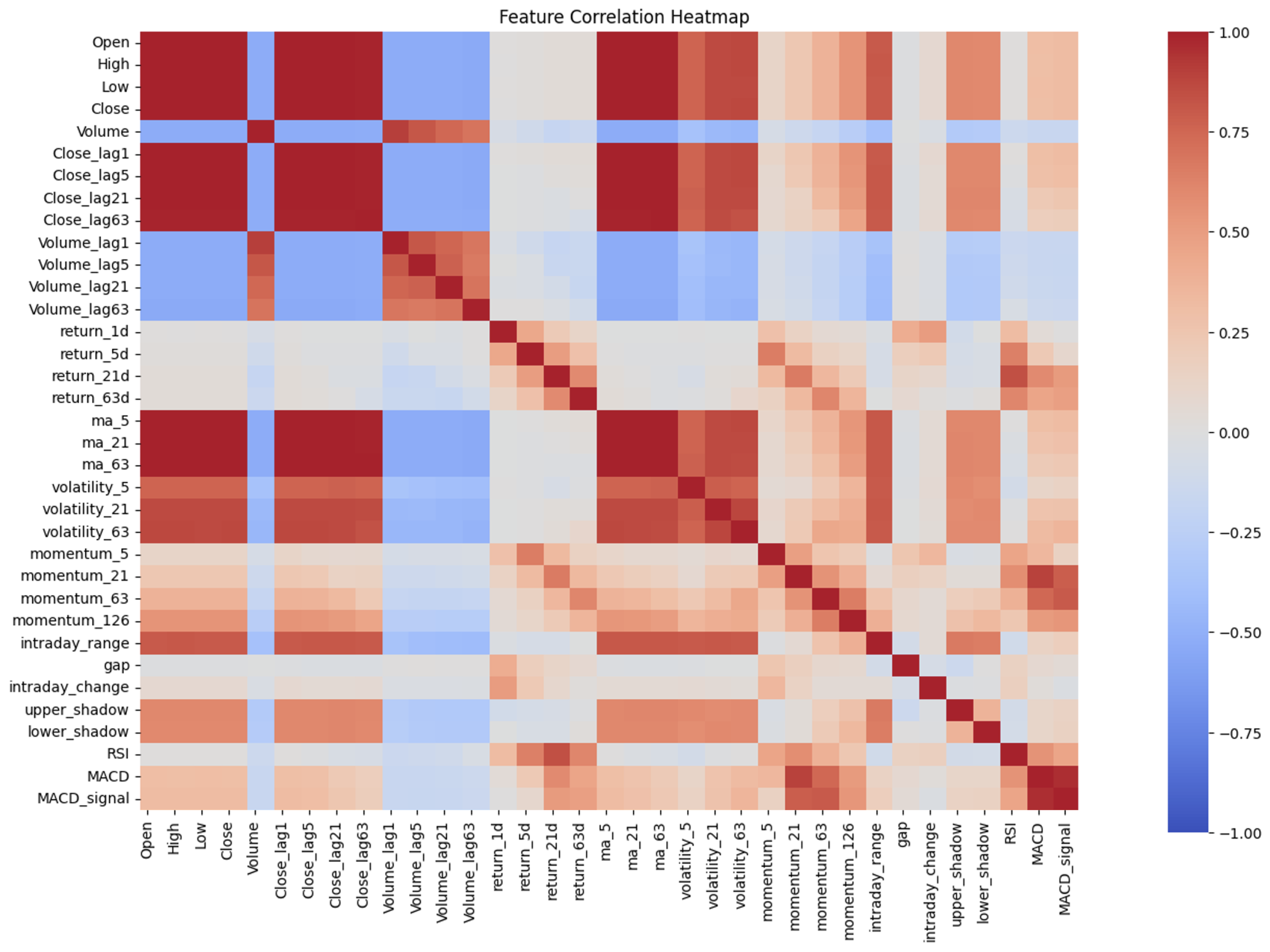
Figure 2.
SPY close price vs. SARIMA’s weekly sliding-window prediction in 2024.
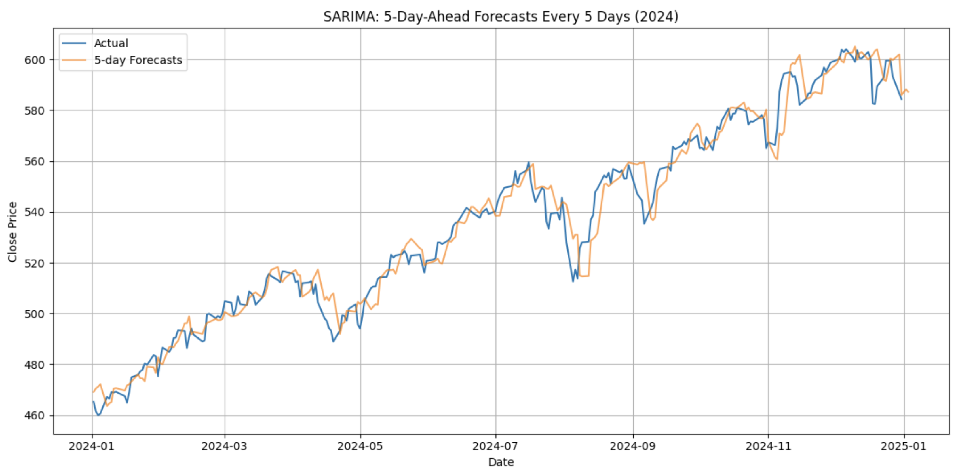
Figure 3.
NVDA close price vs. ETS’s daily rolling-window prediction in 2024.
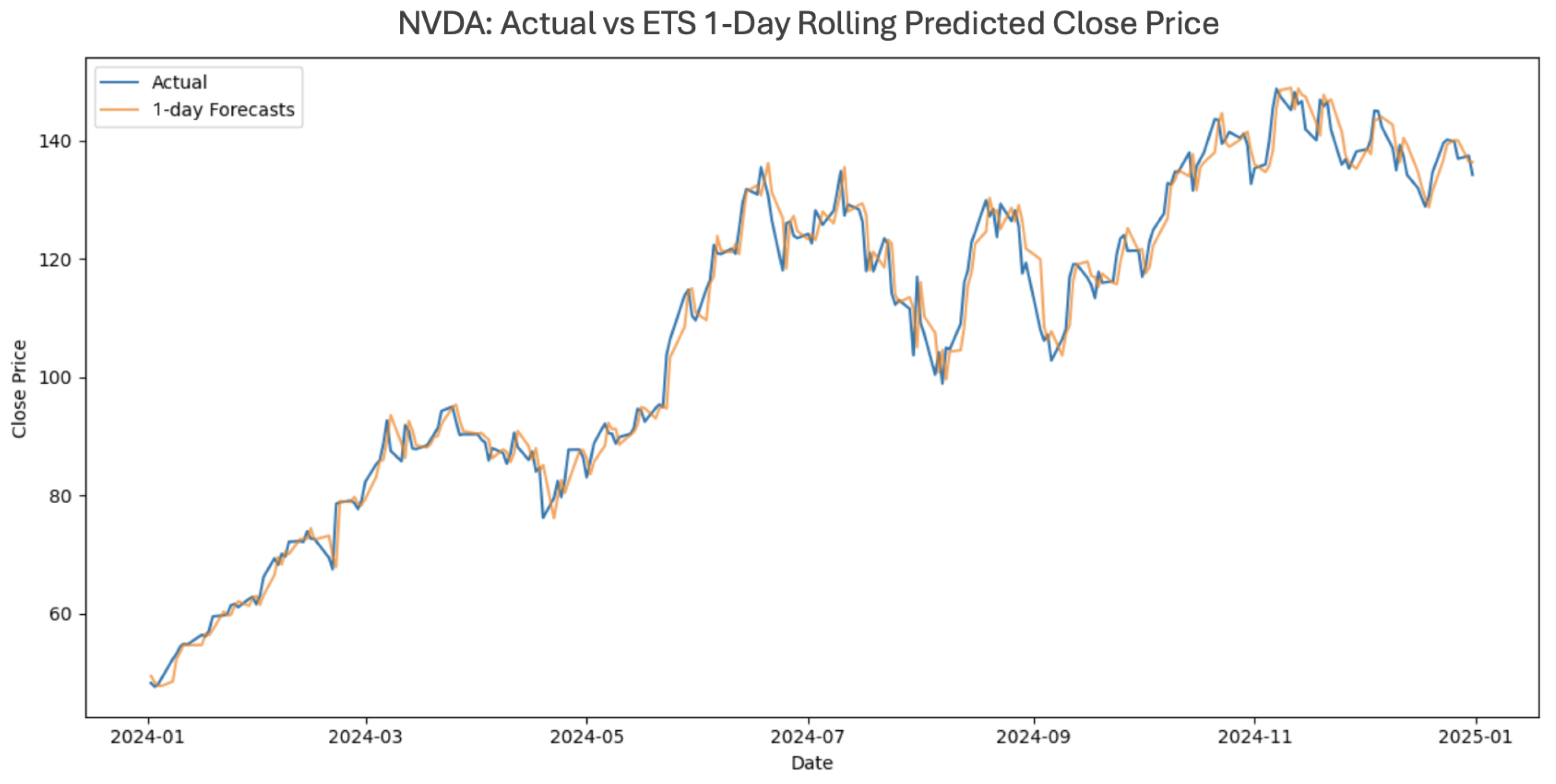
Figure 4.
SPY close price vs. TFT’s daily rolling-window prediction in 2021.
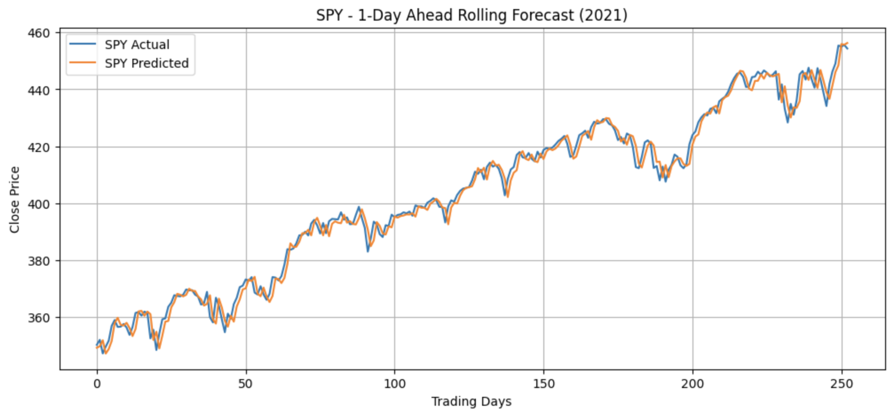
Figure 5.
The TFT model’s interpretability mechanisms: (a) Feature importance and (b) Temporal attention.
Figure 5.
The TFT model’s interpretability mechanisms: (a) Feature importance and (b) Temporal attention.
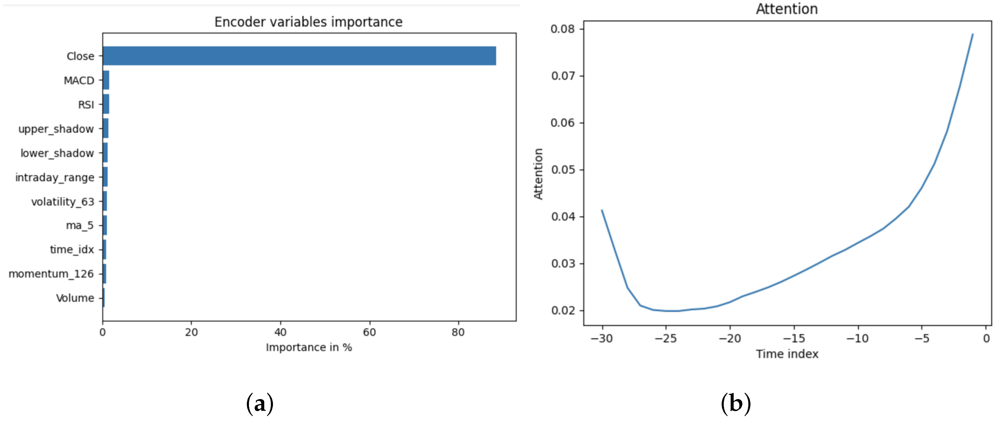
Figure 6.
SPY close price vs. TFT-GNN’s daily rolling-window prediction in 2024.
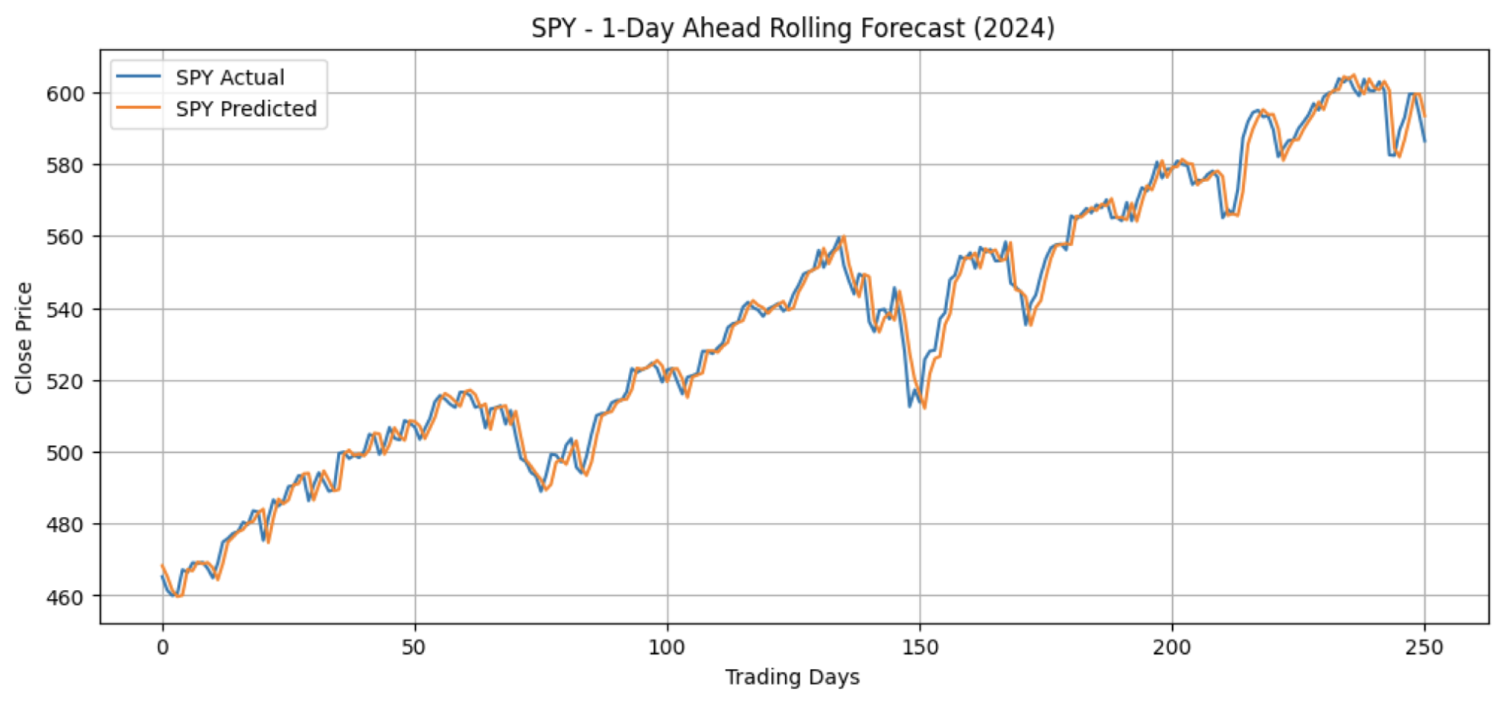
Figure 7.
Feature importance in the TFT-GNN model.
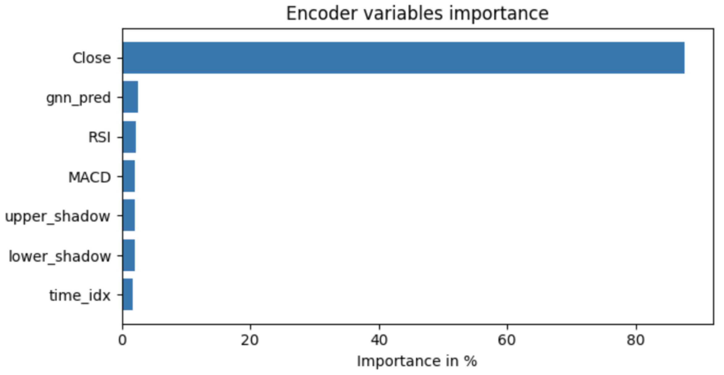

Table 1.
Summary of daily forecasting performance across models.
| Model | RMSE (↓) | (↑) | Horizon | Interpretability | Compute Time |
|---|---|---|---|---|---|
| SARIMA | Weekly | Low | Moderate | ||
| ETS | Daily | Moderate | Low | ||
| TFT | Daily | High | High | ||
| TFT-GNN | Daily | High | Very high |
Disclaimer/Publisher’s Note: The statements, opinions and data contained in all publications are solely those of the individual author(s) and contributor(s) and not of MDPI and/or the editor(s). MDPI and/or the editor(s) disclaim responsibility for any injury to people or property resulting from any ideas, methods, instructions or products referred to in the content. |
© 2025 by the authors. Licensee MDPI, Basel, Switzerland. This article is an open access article distributed under the terms and conditions of the Creative Commons Attribution (CC BY) license (http://creativecommons.org/licenses/by/4.0/).
Copyright: This open access article is published under a Creative Commons CC BY 4.0 license, which permit the free download, distribution, and reuse, provided that the author and preprint are cited in any reuse.


