
Submitted:
17 July 2025
Posted:
21 July 2025
You are already at the latest version
Abstract
The Sustainable Development Goal (SDG) Indicator 11.3.1, defined as the ratio of Land Consumption Rate (LCR) to Population Growth Rate (PGR) and collectively referred to as LCRPGR, is widely used to assess urban land use efficiency (LUE). However, its reliance on two-dimensional built-up area data limits its ability to capture vertical urban growth and spatial form. This study introduces a trajectory-based framework that integrates built-up area (BUA) and built-up volume (BUV) to enhance LUE assessments. By representing urban growth as a trajectory in normalized BUA–BUV space, the framework reveals prevailing built form (horizontal, balanced, or vertical) and directional growth patterns (expansion or intensification) that underlie LUE outcomes. We apply the BUA–BUV trajectory framework to 10,856 urban centers using data from the Global Human Settlement Urban Centre Database (GHS-UCDB 2025) spanning 1980–2020. Results show that horizontal expansion remains the globally dominant growth pattern, with 97% of urban centers classified as horizontally dominant in 2020. Typology analysis reveals that “Sustained Horizontal Growth” accounts for most urban trajectories, while typologies indicative of vertical intensification are rare. Although the global median LCRPGR values declined from 1.67 (1980–2000) to 1.05 (2000–2020), suggesting more proportionate land consumption, trajectory distributions show limited structural transition toward vertical or balanced growth. The findings underscore the limitations of relying on LCRPGR alone to assess LUE in the context of urban sustainability. The BUA–BUV trajectory framework complements SDG 11.3.1 by embedding spatial structure into LUE assessment, distinguishing between structurally divergent paths that yield similar LCRPGR values. This added diagnostic capability supports more informed interpretations of urban growth and can guide planning strategies toward compact, balanced, and sustainable development pathways.
Keywords:
vertical urban growth
; SDG 11.3.1
; land use efficiency
; trajectory framework
; built-up volume
1. Introduction
The Sustainable Development Goal (SDG) indicator 11.3.1, defined as the ratio of the Land Consumption Rate (LCR) to the Population Growth Rate (PGR), collectively referred to as LCRPGR, is a core metric for monitoring land use efficiency (LUE) in urban areas [1]. This indicator supports SDG 11, which aims to “make cities and human settlements inclusive, safe, resilient, and sustainable,” and explicitly addresses Target 11.3, which focuses on enhancing inclusive and sustainable urbanization and strengthening capacities for participatory and integrated human settlement planning [2]. The underlying premise of LCRPGR as a quantitative measure of LUE is that urban areas are considered more efficient when they accommodate population growth without a commensurate or higher increase in land consumption [3]. In this context, efficient land use is closely associated with urban compactness, i.e., a spatial structure where population density is maintained or increased relative to land expansion. The LCRPGR thus serves as an indicator of urban compactness over time [2]. A value near or below one indicates that land consumption is proportionate to or less than population growth, suggesting compact and efficient urban development. Conversely, values substantially larger than one imply that land is being consumed more rapidly than the population is growing, often indicative of urban sprawl and inefficient land use.
Despite its widespread adoption, the current formulation of LCRPGR is inherently limited by its exclusive reliance on two-dimensional representations of built-up area, thereby neglecting the vertical dimension of urban form [3]. Yet, many cities grow by increasing land use intensity, such as building taller structures. In such a context, volumetric data is necessary to reveal patterns of densification and spatial intensity, which are hard to capture with traditional geographic methods that only consider horizontal expansion [4]. Beyond simply classifying urban areas as efficient or inefficient, it is equally important to understand the spatial processes that give rise to these outcomes. Efficiency in land use may stem from horizontal containment, vertical densification, or a combination of both. LCRPGR alone, while helpful in indicating whether land is being consumed efficiently relative to population growth, does not reveal how this efficiency is achieved, nor whether it is sustainable in the long term.
Integrating time-series data on both built-up area and built-up volume offers a more comprehensive basis for interpreting LUE. This dual approach allows for the identification of distinct urban growth typologies that may be overlooked in analyses focused solely on horizontal expansion, particularly in high-density, land-constrained cities where vertical development is the prevailing pattern. The omission of the vertical dimension constrains the ability of LUE assessments to capture the spatial strategies underpinning urban growth fully. For example, a low LCR paired with a high PGR may signal efficient land use. However, the mechanisms, such as upward densification, remain obscured unless vertical development is explicitly accounted for. While challenges remain in producing globally consistent building height or volume data, recent advancements in remote sensing and geospatial technologies offer increasing potential for capturing vertical urban structures. Recently, global-scale 3D data on urban areas, e.g., [5,6,7,8,9,10], capturing building heights and volumes, have become available. Integrating this third spatial dimension is therefore feasible and necessary for producing more accurate, interpretable, and policy-relevant assessments of LUE under SDG 11.3.1.
In this study, we present a novel approach to enhance the analytical value of SDG indicator 11.3.1. Specifically, we introduce and apply a Built-up Area–Built-up Volume (BUA-BUV) trajectory framework that captures the co-evolution of horizontal and vertical dimensions of urban growth. The framework aims to uncover undetected spatial growth typologies in LCRPGR-only analyses by integrating temporal data on horizontal spread and vertical build-up. Examining these trajectories alongside LCRPGR provides a more comprehensive perspective on LUE and urban development outcomes. While not intended to replace existing SDG 11.3.1 primary and secondary indicators, this framework is proposed as a complementary approach that may improve urban LUE assessments’ interpretability and policy relevance.
The proposed method is applied to a globally harmonized dataset, the Global Human Settlement Urban Centre Database (GHS-UCDB) 2025, which includes over 10,000 urban centers with consistent multitemporal records on built-up areas, population, and, importantly, built-up height and volume [11]. This dataset enables the joint analysis of horizontal and vertical growth trends over two key intervals (1980–2000 and 2000–2020) and cumulatively across 1980–2020. These periods were selected to capture long-term urban development patterns before and after the turn of the century, reflecting historical urban expansion and more recent trends influenced by rapid population growth, economic globalization, and vertical urbanization. In line with the 2021 revision of the SDG 11.3.1 metadata, which introduced a simplified change-rate formula for LCR [1], we re-estimate LCR, PGR, and LCRPGR using the updated standard. Previous global studies, e.g., [3,12,13,14], were constrained by older formulations and a lack of vertical metrics. Our approach addresses these limitations by integrating updated LUE estimates with BUA–BUV trajectory analysis, providing a novel framework to assess urban growth’s horizontal extent and vertical intensity as they relate to LUE.
The remainder of the paper is organized as follows. Section 2 reviews related work on urban LUE, particularly emphasizing the limitations of LCRPGR and the emerging importance of incorporating vertical urban metrics and typologies. Section 3 revisits the SDG Indicator 11.3.1 and introduces the conceptual basis for integrating BUA–BUV trajectories with SDG Indicator 11.3.1. Section 4 presents the application of the proposed BUA–BUV trajectory framework, detailing the data sources, derivation of LCR, PGR, and LCRPGR, and the methodological procedures for classifying urban growth trajectories using time-series data on built-up area and volume. Section 5 presents the empirical findings, followed by a discussion in Section 6. Section 7 concludes the paper with implications and directions for future research.
2. Related Work
Since the adoption of the UN SDGs in 2015, a growing body of research has examined LCRPGR across multiple spatial scales to evaluate urban LUE and to understand diverse urban development trajectories worldwide [12,13,14,15,16,17,18,19,20,21,22,23,24,25,26,27,28,29,30,31]. These studies reveal a wide range of urban growth patterns and LUE outcomes, shaped by factors such as population size, expansion rate, urban form, and spatial configuration. Collectively, the findings highlight the need for context-specific land use policies that account for the complex and spatially varying dynamics between land consumption and population growth.
Despite its widespread use, LCRPGR suffers from key conceptual and methodological limitations. A single LCRPGR value can correspond to markedly different urbanization scenarios—for example, extensive land expansion alongside population decline, or minimal spatial growth during rapid population increase [1,3,15,16,22,23,32,33]. Such ambiguities become more pronounced at aggregated spatial scales, where intra-urban variation is masked [12,13,16,34,35,36]. To mitigate these issues, researchers have made use of categorization frameworks based on LCR and PGR combinations [3,13,14,17]. The categorization of the LCRPGR improved its interpretability by distinguishing the drivers of efficiency, i.e., between built-up land consumption and population growth. Additional metrics, such as Built-up Area per Capita (BUpC), Total Change in Built-up Area, Abstract Achieved Population Density in Expansion Areas (AAPDEA), and Marginal Land Consumption per New Inhabitant (MLCNI), have also been introduced to capture the form and intensity of urban expansion more effectively [1,13,14]. In parallel, the indicator framework has been extended to account for economic and governance factors [17,37], while advancements in Earth Observation (EO) and population data, combined with uncertainty quantification techniques, have enhanced the reliability and comparability of LCRPGR estimates [16,38,39,40].
Despite these efforts, a key dimension of urban growth remains largely overlooked in the current SDG 11.3.1 framework: the vertical dimension of urban development. Existing LCRPGR estimation approaches rely exclusively on two-dimensional representations of built-up areas, focusing solely on horizontal land expansion while neglecting the vertical dimension of urban form [3]. The need to include the vertical dimension in LUE assessments is clearly shown in the findings of Estoque et al. [3]. Their global analysis of LUE patterns found that the correlation between LCR and PGR varies across countries. In many cases, the correlation was strong and positive. However, the correlation was weak or not present in several high-income and very high human development countries. The authors suggested that in these places, population growth may have been absorbed not by expanding outward, but by building upward. The widespread presence of high-rise buildings in these areas supports this idea. This kind of vertical growth is not captured by current LCRPGR methods, which focus only on horizontal land expansion.
In contrast, several studies outside the SDG 11.3.1 framework underscore incorporating vertical metrics to assess urban form and LUE more comprehensively. For instance, Mahtta et al. [41] demonstrated that combining horizontal and vertical growth indicators reveals diverse urban expansion typologies, such as outward budding, stabilization, or simultaneous upward and outward growth. Similarly, Soltani et al. [42] applied an integrated 2D–3D spatial analysis to metropolitan regions and identified context-specific phenomena, including “vertical sprawl” in peripheral zones and polycentric vertical intensification. Ruan et al. [43] used building height data to assess built-up land intensity and its association with LUE, identifying areas of both underutilization and overconcentration. Complementing these efforts, several metrics have been developed to capture vertical urbanization systematically. Zambon et al. [44] introduced the Vertical-to-Horizontal Growth (VHG) ratio to discriminate vertical from horizontal urban expansion; Ghosh et al. [45] proposed the Built-up Volume per Capita (BUVpC) as a measure of spatial inequality; Ruan et al. [43] calculated a Coupling Index to examine mismatches between built-up land intensity and efficiency; and Kim & Kim [46] developed a 3D Land Use Index (3D LUI) to quantify vertical land use. These studies highlight that excluding vertical indicators from existing LUE assessments may obscure critical spatial dynamics. Integrating 3D metrics is therefore essential to improve LUE assessments’ interpretability and policy relevance, particularly under the SDG 11.3.1 framework.
Recent studies further emphasize the growing significance of considering vertical urban development in LUE assessment. Liu et al. [47] documented a widespread increase in the vertical use of space over recent decades (1985-2015), highlighting the uneven distribution of building volume across cities. This finding was complemented by Frolking et al. [48], who identified a global shift from predominantly lateral expansion to upward growth in the 1990s to the 2010s, with particularly pronounced vertical intensification observed in many Asian urban centers. These transitions indicate that urban expansion is no longer a purely horizontal phenomenon but increasingly reflects a complex interplay between outward spread and upward development [42]. This shift toward vertical urban development further highlights the need to extend SDG 11.3.1-based LUE assessments beyond two-dimensional metrics.
Numerous typologies and trajectory-based frameworks have been developed in urban studies to characterize the direction, rate, and nature of spatial growth. These include methods that track the outward expansion of urban edges, analyze growth from city centers, or classify patterns such as infill, leapfrog, and edge expansion, among others [49,50,51,52,53]. Some studies have examined the co-evolution of built-up area and population over time, e.g., [54]. These trajectory patterns have also been linked to LUE assessments within the framework of SDG 11.3.1 [3,13,30], helping to determine whether spatial entities (e.g., cities, countries) are simultaneously expanding in both dimensions, growing in area despite population decline, or densifying through population growth with minimal spatial expansion. However, all these cited frameworks and approaches remain limited to the horizontal dimension of urban growth.
The 2D–3D typology proposed by Mahtta et al. [41] is the most analogous to the present study in its consideration of vertical urban growth. Their approach combines GHSL-derived built-up extent with microwave backscatter data—used as a proxy for building height—and incorporates population data to classify urban expansion patterns. The authors identified five typologies through cluster analysis of temporal changes in built-up area and backscatter intensity: stabilized, outward, mature upward, budding outward, and upward and outward growth. A related study by Frolking et al. [48] similarly integrates backscatter and built-up area data, categorizing urban growth based on the rates of change in built fraction and backscatter signal. Their typology includes growth modes such as slow growth, outward growth, rapid 3D or up-and-out growth, and height-dominant or upward growth. While both studies provide valuable insights into global urban growth patterns and built form evolution, their focus remains on characterizing development patterns rather than evaluating LUE. Moreover, their reliance on microwave backscatter as a vertical proxy, which before the launch of Sentinel 1 was limited in temporal availability and spatial resolution, constrains their applicability for more recent periods or finer-scale analyses. Additionally, the use of clustering methods introduces a degree of methodological subjectivity, as the absence of standardized criteria for defining clusters reduces the replicability of results across datasets and geographic contexts.
Another closely related study is by Liu et al. [47], who developed a global 3D urban morphology typology using GUS-3D data. Their framework analyzes the relationship between building horizontal coverage ratio (as a measure of horizontal density) and average building height (as an indicator of vertical intensity) to classify cities into built-form types such as sparse-low rise, compact-low rise, sparse-high rise, and compact-high rise. This typology provides a valuable means of characterizing prevailing structural configurations of urban form across diverse global contexts. While their proposed typology yields essential insights into spatial variation in built forms, it was not extended to capture temporal dynamics in urban growth trajectories or explicitly applied to LUE assessment.
To summarize, although LCRPGR has become a widely adopted indicator for assessing LUE, its current formulation remains limited to two-dimensional analyses that overlook the vertical component of urban growth. This omission hinders the ability to differentiate between diverse spatial development patterns, particularly in dense urban contexts where vertical expansion could be evident. While prior studies have introduced typologies incorporating vertical metrics, these approaches are either not directly linked to the SDG 11.3.1 framework or lack temporal depth and methodological standardization. Moreover, reliance on proxies such as microwave backscatter and clustering-based classifications constrains replicability and spatial resolution. This study addresses these limitations by introducing a BUA–BUV trajectory framework that captures the co-evolution of horizontal and vertical urban growth using harmonized multitemporal data on built-up area, built-up volume, and population from the GHS-UCDB 2025. By integrating this trajectory framework with updated LCRPGR estimates, the study provides a scalable, interpretable, and policy-relevant method for enhancing SDG 11.3.1-based urban LUE assessments.
3. Integrating BUA–BUV Trajectories with SDG 11.3.1
3.1. Revisiting SDG Indicator 11.3.1
The fundamental formulae for computing indicator 11.3.1 (LCRPGR) and its components are presented below, based on the latest metadata definitions [1] with minor modifications to ensure consistency in variable notation.
In the above formulae, BUA and Pop are the total built-up area and population at two epochs ( and ), respectively; Δt is the time interval between epochs. In the context of SGD 11.3.1, built-up areas are defined as all areas occupied by buildings [1].
Interpreting an LCRPGR value requires understanding the sign and relative magnitude of LCR and PGR. This indicator is designed to assess whether the spatial expansion of urban areas is aligned with population dynamics. A structured classification of LCRPGR values across all combinations of LCR and PGR sign and magnitude is presented in Table 1. While this typology facilitates a systematic interpretation of LUE, it remains inherently two-dimensional, limited to changes in surface area and demographic growth. As such, it does not provide insight into the underlying spatial morphology of urban expansion, particularly whether a given LCRPGR outcome is associated with predominantly horizontal sprawl, vertical densification, or a hybrid of both. This limitation underscores the need for a more spatially expressive framework to capture the co-evolution of urban extent and structural form.
3.2. The BUA-BUV Trajectory Framework
3.2.1. Constructing the BUA-BUV Trajectory
The framework conceptualizes urban growth as a trajectory in a two-dimensional space, with the x-axis representing and the y-axis representing . For each urban center , a trajectory is constructed as an ordered sequence of observations across temporal snapshots , , …, , where each () denotes a specific year or epoch. The raw trajectory is defined as:
The resulting trajectory, illustrated in Figure 1a, represents the temporal co-evolution of urban spatial extent and built volume as a sequence of connected line segments in BUA–BUV space. Each segment, constructed by linearly linking consecutive observations, conveys the direction and magnitude of growth between time steps, thereby enabling the interpretation of growth modality, whether horizontal, vertical, or mixed, across urban centers and temporal intervals.
To allow for meaningful comparison of growth patterns across urban centers, the and values are linearly min–max normalized across all urban centers and all time steps, producing a normalized trajectory (Figure 1b). The normalized values for each time step are computed as:
where , , , and are computed from the full spatiotemporal dataset of all urban centers and all time points. This normalization ensures that each center’s trajectory is evaluated relative to the observed global distribution of and values.
3.2.2. Interpreting the Normalized Trajectory Space
In the normalized space (Figure 1b), the position of an urban center’s trajectory relative to the angle bisector (called 1:1 line in the following, where ) reflects its prevailing urban form compared to others in the global dataset. It is essential to clarify that the 1:1 line in the normalized plot does not correspond to equal absolute changes in BUA and BUV in the original units (e.g., km2 vs. km3). Instead, it reflects equal relative growth with respect to each variable’s maximum range within the sample. As such, the 1:1 line serves as a conceptual reference for identifying the dominant direction of structural change: trajectories lying above the line indicate relatively larger vertical growth (i.e., BUV increased more, proportionally, than BUA), suggesting vertical intensification; those below the line reflect dominant horizontal expansion; and those along the line imply a proportionally balanced increase in both horizontal and vertical dimensions. Because normalization is performed across the global sample, the resulting positions are inherently comparative and highlight relative differences in urban morphological trajectories, rather than absolute physical equivalence.
Trajectory direction between two epochs reveals the mode of growth. This direction is quantified by computing the slope of its trajectory in normalized BUA–BUV space, i.e., by measuring the counterclockwise angle between the x-axis and the line segment connecting the trajectory’s earliest and latest time points. A rather horizontal movement (increase in BUA with limited BUV change) indicates horizontal expansion. An upward direction reflects vertical intensification. Diagonal movements, where both BUA and BUV increase, capture combined or balanced growth, with the slope indicating relative dominance: shallower slopes (e.g., 0°–30° from the BUA axis) point to area-driven growth, moderate slopes (e.g., 30°–60°) suggest balanced expansion, and steeper slopes (e.g., 60°–90°) denote volume-led densification.
These spatial trajectories can be categorized into growth typologies (Table 2), which describe the existing built form and its evolution. For example, trajectories above the 1:1 line with steep upward directions reflect intensifying verticality, while shallow movements in the same region indicate outward spread within a vertical context. Similarly, trajectories near the 1:1 line may reinforce balance or shift toward vertical or horizontal dominance. Below the line, upward movements may signal early densification from a low-rise base, whereas persistently shallow angles confirm sustained horizontal sprawl.
It is possible to summarize these trajectories using a single scalar, such as the angle between the overall trajectory vector and the 1:1 line. However, we refrain from such reduction, as it would obscure critical aspects of urban development, particularly the initial built form and potential shifts in growth direction across epochs, that are better captured by analyzing the full sequence of temporally ordered segments. For instance, an urban center that begins with a vertically dominant form (above the 1:1 line) and undergoes moderate horizontal expansion may yield a trajectory angle suggesting horizontal growth, even though its structural configuration remains predominantly vertical. This loss of contextual detail limits the interpretability of scalar metrics in capturing dynamic urban processes. By preserving the full trajectory in the normalized BUA–BUV space, the framework enables a more comprehensive understanding of prevailing morphology and growth direction, which is essential for assessing the structural drivers behind LUE outcomes.
The preceding discussion illustrates the BUA–BUV framework graphically for interpretability. However, it is not limited to visual inspection. The analytical underlying concept is operationalized through quantitative calculations of trajectory properties such as changes in normalized BUA and BUV, growth vector direction or trajectory angle, and position relative to the 1:1 reference line. These metrics can be used to automate classification into typologies, detect shifts in growth modality, or compare urban centers across time and space.
The trajectory framework remains applicable even when either BUA and/or BUV decreases over time, as it is fundamentally designed to capture relative structural change rather than assume unidirectional growth. Although the present study illustrates trajectories primarily within the context of simultaneous increases in BUA and BUV, a scenario commonly observed in global urban centers undergoing expansion, this choice was made for interpretive clarity. In cases where reductions occur in either or both dimensions, such as in the aftermath of natural disasters, armed conflict, or deliberate urban downsizing, the framework can still characterize the structural implications of such changes. For instance, a downward or leftward trajectory in the normalized space would reflect vertical decline (or de-densification) and horizontal contraction, respectively. These movement patterns can be assigned corresponding typologies that denote regression or reversal in urban development. Thus, the BUA–BUV trajectory framework is inherently flexible and capable of representing diverse urban change dynamics, including atypical or negative growth scenarios, as long as the temporal sequence and normalization procedures are preserved.
3.2.3. Interpretation in the Context of SDG Indicator 11.3.1
The BUA-BUV trajectory-based typologies, when used in conjunction with LCRPGR, provide a more comprehensive basis for evaluating LUE and its alignment with sustainable urban development within the context of SDG 11.3.1. As discussed previously, the LCRPGR does not convey the spatial form or character of urban growth. The typologies address this limitation by describing how horizontal and vertical development evolve together over time.
Urban centers with similar LCRPGR values may belong to different trajectory typologies, and vice-versa. Referring to our hypothetical example (Figure 1), City A and City I might both fall within the “efficient” range (0 < LCRPGR ≤ 1), yet their growth typologies diverge significantly. City A’s steep trajectory above the 1:1 line indicates vertical intensification and compact urban form. At the same time, City I follows a shallow path below the line, suggesting continued horizontal expansion with minimal vertical development. Although both may appear equally efficient numerically according to the SDG 11.3.1 standard, their long-term sustainability implications differ: City A’s compact form supports resource efficiency and reduced land consumption, whereas City I may incur higher infrastructure costs and contribute to urban sprawl.
Conversely, cities with similar spatial trajectories may exhibit varying LCRPGR values depending on their population growth dynamics. For instance, City G shows a steep upward trajectory from a low-rise base—suggesting a vertical correction or densification strategy—yet may still have an LCRPGR larger than one if its population growth remains stagnant. In such a case, the indicator might not yet reflect this progress despite the improving spatial form.
These distinctions highlight the importance of interpreting LCRPGR with BUA–BUV typologies. The trajectories serve as a spatial diagnostic tool that explains how a particular efficiency level was achieved and whether the pathway is structurally sustainable.
As a prerequisite, the analyses presented here assume that the underlying BUA and BUV data are free from blunders and outlier. The procedures for detecting and removing such anomalies are described in the next section, where we apply the proposed framework to assess urban growth trajectories across a global sample of urban centers.
4. Application of the BUA-BUV Trajectory Framework for Enhanced LUE Assessment of Global Urban Centers
4.1. Data Description
To demonstrate the empirical usefulness of the BUA–BUV trajectory framework, we applied it to a globally standardized dataset of urban centers derived from the Global Human Settlement Urban Centre Database (GHS-UCDB), developed by the European Commission’s Joint Research Centre [11]. The latest release, GHS-UCDB R2024A, also called GHS-UCDB 2025, provides a harmonized, spatially explicit dataset of 11,422 urban centers globally. These are delineated as polygons and defined according to the Degree of Urbanisation (DEGURBA) methodology, requiring a minimum population of 50,000 and a density of at least 1,500 inhabitants per km2 of permanent land [55]. Each entry is further annotated with its corresponding country, UN SDG Region, and World Bank income classification.
Each urban center in the database has multitemporal attributes on built-up area and population from 1975 to 2020 in 5-year intervals, along with projections for 2025 and 2030. It also provides average built-up height estimates for 2020 and corresponding built-up volume data for historical and projected periods, allowing for a three-dimensional assessment of urban growth. The core variables are derived from four key layers of the GHSL Data Package 2023 [56], all at 100-m spatial resolution: GHS-BUILT-S for built-up surface area [57], GHS-POP for population [58], GHS-BUILT-H for building height [8], and GHS-BUILT-V for built-up volume [7]. GHSL estimates are among the most accurate among publicly available datasets, with built-up area errors averaging 6% per 100-m pixel, a mean absolute error of 2.27 meters for building height, and over 80% accuracy for population estimates [59].
4.2. Data Processing
This study primarily utilized two files from the GHS-UCDB 2025: a spreadsheet in Microsoft Excel format (GHS_UCDB_THEME_GHSL_GLOBE_R2024A.xlsx) and a Geopackage file (GHS_UCDB_THEME_GHSL_GLOBE_R2024A.gpkg). The GeoPackage, which includes the centroids and boundaries of urban centers, was used primarily for mapping and geovisualization. The spreadsheet served as the primary data source for the analytical components of the study. LCR, PGR, and LCRPGR were computed for each urban center across two multi-decadal periods (1980–2000 and 2000–2020) and over the whole 40-year period from 1980 to 2020, following the formulations in equations (1) to (3). As stated earlier, multi-decadal intervals were intended to capture long-term urban development patterns, as shorter intervals (e.g., 5 years) may be less reliable due to data precision limits and may not reflect substantial changes.
A preliminary statistical examination of the computed LCR and PGR values was performed to assess their distributional properties and identify potential anomalies. For each metric and analysis period (i.e., 1980–2000, 2000–2020, and 1980–2020), descriptive statistics, including minimum, maximum, mean, median, and standard deviation, were computed, and frequency distributions were generated to visualize the overall patterns. The resulting distributions were highly skewed and exhibited substantial deviations from a normal distribution. Specifically, LCR values spanned an extensive range exceeding 4,000, while PGR values ranged up to 54%, which are implausible in realistic urban development contexts, particularly given that these metrics represent annual rates. It is hypothesized that these anomalous values may be attributed to uncertainties or inconsistencies in the built-up area and population estimates. To ensure the robustness of subsequent analyses, a systematic outlier detection procedure based on the modified Interquartile Range (IQR) method [60] was employed to identify and exclude extreme values. A value was classified as an extreme outlier if it fell outside the acceptance range defined as:
where and represents the first (25th percentile) and third (75th percentile) quartiles, respectively; ; and is the total number of observations. This procedure was applied separately to the LCR and PGR distributions across the three analysis periods: 1980–2000, 2000–2020, and 1980–2020. For each metric, the acceptance range was computed based on all available observations ( = 11,422). An urban center was flagged as an outlier and excluded from further analysis if it exhibited at least one LCR or PGR value across any of the three periods that fell outside the corresponding acceptance range. Following this quality control procedure, a sample of 10,856 urban centers was retained for subsequent analysis (Figure 2).
4.3. Trajectory Analysis
Normalization was conducted using the global minimum and maximum BUA and BUV values observed across all three years (1980, 2000, and 2020) using equations (5) and (6). This approach ensures that all trajectory points are mapped to a common normalized space, allowing for direct comparability of spatial position and growth direction across intervals and urban centers.
To characterize the prevailing built form of urban centers at each time point, trajectory points in the normalized BUA–BUV space were categorized based on their position relative to the 1:1 line, representing structural balance between horizontal extent and vertical intensity. As previously described, points above this line indicate a predominance of vertical development, while those below reflect a horizontally extensive built form. To identify cases of structural balance, a strict threshold was applied by computing the 5th percentile of all absolute orthogonal distances to the 1:1 line across the dataset. This threshold defines a narrow band around the 1:1 line within which built-up area and volume are nearly equal, and such points were classified as balanced. Points falling outside this threshold were classified as vertically dominant or horizontally dominant, depending on the sign of the deviation. The 5th percentile was chosen to provide a conservative yet data-driven criterion: stricter thresholds, such as the 1st percentile, may exclude valid balanced cases due to data uncertainty, while broader thresholds like the 10th percentile risk misclassifying structurally unbalanced forms as balanced. This approach ensures interpretive clarity and analytical consistency across time and space.
This study analyzed three temporal intervals: 1980–2000, 2000–2020, and 1980-2020. As described earlier, the slope of each segment was used to classify growth patterns into three directional typologies: slopes between 60° and 90° indicated vertical intensification, 30° to 60° corresponded to balanced growth, and 0° to 30° represented horizontal expansion. Although a universal standard does not exist for such thresholds, these angular divisions were selected to partition the 0°–90° range evenly into three interpretable growth regimes.
4.4. Evaluating LUE Patterns Across BUA–BUV Trajectories
Given the observed skewness in LCR, PGR, and LCRPGR distributions, median values of each of these metrics were used to summarize their respective central tendencies. The relationship between LUE and urban growth typologies was examined by analyzing the computed LCRPGR values in relation to the nine BUA–BUV trajectory categories (Table 2), defined by the combination of built form classification (vertical, balanced, horizontal) and growth direction (vertical intensification, balanced growth, horizontal expansion). Each urban center was assigned to a typology for the three study periods: 1980–2000, 2000–2020, and 1980–2020. The frequency distribution of these nine trajectory typologies was then analyzed across periods, UN SDG Regions, and World Bank Income Groups.
Since all urban centers exhibited positive LCR values across all analysis periods, indicating continuous expansion of built-up areas, it became more straightforward to interpret LUE by classifying LCRPGR values. Prior global studies, e.g., [3,12,14], have used five LCRPGR categories (≤ –1, –1 to 0, 0–1, 1–2, and > 2) to capture varying efficiency levels. This study adopts a three-class scheme to simplify capturing the relationship between growth trajectories and LUE. Specifically, LCRPGR values were categorized as ≤ 0 (inefficiency due to land expansion despite population decline or stagnation), 0–1 (efficient growth), and > 1 (inefficiency where land consumption outpaces population growth). For each trajectory typology, the number of urban centers falling within each LCRPGR category was computed to examine how structural and directional growth patterns relate to efficiency outcomes.
Where relevant, results are interpreted in the context of UN SDG Regions and World Bank Income Groups to account for broader regional and economic patterns influencing urban development and efficiency.
5. Results
5.1. BUA-BUV Trajectories and Prevailing Built Form
The co-evolution of BUA and BUV from 1980 to 2020 is illustrated in Figure 3, which includes all urban centers (panels a–b) and the top 10 most populous urban centers (panels c–d). In the raw BUA–BUV space (panels a and c), cities such as Tokyo, Guangzhou, and Shanghai exhibit long trajectories extending toward the upper-right quadrant, indicating substantial absolute increases in both BUA and BUV. However, this representation primarily captures the scale and cumulative magnitude of growth, providing limited insight into each urban center’s prevailing built form and directional characteristics relative to others. This plot alone is insufficient for reliably classifying urban centers by urban growth trajectory, at least not in a systematic or replicable manner. While it offers a visual impression of how built-up area and volume have co-evolved between 1980 and 2020, it lacks grouping or defined typological criteria. As a result, relying solely on visual inspection can lead to subjective and potentially inconsistent classifications.
Normalized trajectories (panels b and d), which rescale growth to a standard 0–1 range, allow for more meaningful comparisons across urban centers of varying size. Aided by the 1:1 line, these plots reveal heterogeneous developmental pathways. Some urban centers show steep upward trajectories aligned with vertical intensification, while others follow flatter paths consistent with horizontal expansion. For example, among the top 10 most populous cities, Tokyo, Guangzhou, and Seoul exhibit vertically oriented trajectories followed by lateral extension. Jakarta, Dhaka, and Manila maintain relatively flat trajectories indicative of sustained horizontal growth. These contrasting patterns highlight the interpretive value of the trajectory framework in distinguishing spatial development strategies that are not readily discernible using absolute values alone.
Figure 4 illustrates the evolving spatial distribution of prevailing built form types, while the corresponding numerical distributions are provided in Supplementary Tables S2 and S3. In 1980, most urban centers—9,306 or 86%—were classified as horizontally dominant, while 1,172 (11%) exhibited a balanced built form, and only 378 (3%) were vertically dominant. Horizontally dominant urban centers were geographically widespread, occurring across various SDG regions. In contrast, urban centers with balanced built forms were disproportionately concentrated in Asia, accounting for 76% of all balanced urban centers globally. Notably, Asia also hosted the highest number of vertically dominant urban centers, with 323 out of the 378 located primarily in countries such as China, Japan, and South Korea. By 2020, the proportion of horizontally dominant urban centers had increased to 97% (or 10,528 urban centers), while the shares of balanced and vertically dominant centers declined to 1% and 2%, respectively, both categories remaining primarily concentrated in Asia. These shifts indicate a consistent global trajectory toward horizontal urban form over the four-decade period.
5.2. Trajectory Typologies of Urban Centers
Trajectory typologies derived from the normalized BUA–BUV space (Figure 3b) and their corresponding spatial distributions (Figure 5; Supplementary Tables S4–S9) reveal the dominant structural evolution pathways of urban centers. Over the 1980–2000 and 2000–2020 intervals, “Sustained Horizontal Growth” (Typology I) was the most common growth pattern. This typology accounted for 6,307 (58%) urban centers in the earlier period, and rose to 74% in the latter, reinforcing horizontal expansion as the prevailing global trend. In both periods, urban centers in “Central and Southern Asia”, “Eastern and South-Eastern Asia”, and “Sub-Saharan Africa” collectively accounted for over 60% of all cities exhibiting this growth pattern.
“Moving Toward Vertical Balance” (Typology H) was the second most common growth pattern, accounting for 28% of urban centers in 1980–2000, but declining to 20% in 2000–2020. During the first period, this typology was concentrated mainly in “Eastern and South-Eastern Asia” and “Europe”, comprising approximately 53% of all urban centers in this category. By the end of the second period, “Eastern and South-Eastern Asia” significantly expanded its share, representing about 48% of urban centers under this typology. At the same time, most other regions experienced a decline in their numbers.
Typologies indicative of more structurally balanced or transitional growth, such as “Sustained Balanced Growth” (Typology E) and “Transitioning to Horizontal Growth” (Typology F), were relatively uncommon. Typology E, mostly observed in “Eastern and South-Eastern Asia”, declined from 6% to 2% between the two periods. Typology F similarly decreased from 5%, primarily concentrated in “Central and Southern Asia” and “Sub-Saharan Africa”, to just 0.7%.
Typologies associated with substantial vertical intensification (A: Vertical Intensification, D: Transitioning to Vertical Growth, and G: Vertical Rise from Horizontal Base) were absent in both periods. Typology B (Balanced Growth in Vertical Context) was observed in approximately 3% of all urban centers in both periods. This typology was heavily concentrated in “Eastern and South-Eastern Asia”, which accounted for over 80% of all urban centers classified under it. Typology C (Horizontal Expansion in Vertical Context) was observed in only 6 (or 0.06%) urban centers in 2000–2020, all located in “Eastern and South-Eastern Asia” and in “Europe”. These findings point to the limited adoption of vertical growth trajectories on a global scale.
5.3. Temporal Trends in LCR, PGR, and LCRPGR
The temporal dynamics of the SDG 11.3.1 metrics are summarized in Table 3, which presents values for all urban centers and further disaggregates the results by UN SDG Regions and World Bank Income Groups for additional context.
Between 1980–2000 and 2000–2020, the global median LCR decreased from 3.47% to 1.72%, indicating a notable deceleration in horizontal land expansion. The median PGR also declined, from 1.97% to 0.95%, though at a slower rate. Consequently, the median LCRPGR dropped from 1.67 to 1.05, suggesting improved alignment between land consumption and population growth. When evaluated over the full 1980–2020 period, the global median LCR remained high at 3.44%, while the median LCRPGR reached 1.94.
At the regional level, most SDG regions exhibited decreasing LCR and PGR values from 1980–2000 to 2000–2020. For instance, “Europe” showed persistently low PGR values and relatively high LCRPGR, especially in the earlier period. “Eastern and South-Eastern Asia” and “Central and Southern Asia” exhibited high LCRs in 1980–2000, followed by substantial reductions in 2000–2020. In contrast, “Sub-Saharan Africa” and “Northern Africa and Western Asia” sustained high LCRs and PGRs in both periods, resulting in LCRPGR values near or slightly above 1. Meanwhile, “Oceania”, “Northern America”, and “Australia and New Zealand” showed declining median LCR and PGR values, with median LCRPGR ratios consistently below 1 in the later period.
Across income groups, the global trend of declining LCR and PGR was again evident. High-income urban centers showed the lowest median values in both indicators, with a median LCRPGR of 0.60 in 2000–2020, indicative of compact growth under demographic stability for this period. Lower-middle-income urban centers exhibited the highest LCRPGR values in all periods, including a 1980–2020 median value of 2.48, denoting continued inefficiency. Despite demonstrating high LCR and PGR, low-income urban centers showed improved efficiency over time, with median LCRPGR decreasing from 1.43 to 0.82. Upper-middle-income urban centers showed a more balanced trajectory, with LCRPGR nearing 1.00 in the later period. Over the full period, the median LCRPGR values suggest that LUE does not increase monotonically with income level.
Figure 6 shows the spatial distribution of urban centers by LCRPGR class; their corresponding numerical distributions are provided in Supplementary Figures S3–S5 and Supplementary Tables S10 and S11. Inefficient growth (LCRPGR > 1) was the predominant pattern across all periods, comprising 7,442 urban centers (69%) from 1980–2000 and 5,610 (52%) from 2000–2020. In both intervals, most of these inefficient urban centers were concentrated in “Central and Southern Asia” and “Eastern and South-Eastern Asia,” totaling 4,278 in 1980–2000 and 3,329 in 2000–2020—more than twice the combined number in “Northern Africa and Western Asia,” “Latin America and the Caribbean,” and “Europe.” While the number of urban centers with LCR exceeding PGR declined over time, many did not transition to efficiency; instead, a portion remained inefficient due to persistently high LCR despite demographic decline. The share of urban centers experiencing inefficiency driven by demographic decline (LCRPGR ≤ 0) increased from 1,009 (9%) in 1980–2000 to 2,121 (20%) in 2000–2020. Most of these cases were in “Europe” and “Eastern and South-Eastern Asia,” although the increase in the latter period was significantly influenced by rising numbers in “Sub-Saharan Africa” and “Central and Southern Asia.” The share of urban centers classified as efficient (0 < LCRPGR ≤ 1) was significantly lower than the combined shares of the two inefficient classes. In 1980–2000, only 2,405 urban centers (22%) were considered efficient, with a modest increase to 3,125 (29%) in the 2000–2020. Across both intervals, the highest numbers of efficient urban centers—each exceeding 300—were observed in “Eastern and South-Eastern Asia,” “Latin America and the Caribbean,” “Northern Africa and Western Asia,” and “Sub-Saharan Africa.”
Complementing the spatial distribution (Figure 6), Figure 7 presents the relative composition of LCRPGR classes across SDG regions and income groups. It highlights how inefficient urban growth (LCRPGR > 1) remained dominant in most regions, particularly in lower-middle-income countries, while efficiency became more common in several regions during 2000–2020. The figure also underscores the rising share of urban centers experiencing inefficiency due to demographic decline (LCRPGR ≤ 0), especially in upper-middle and high-income countries.
5.4. Linking Urban Growth Typologies to Efficiency Outcomes
Figure 8 illustrates the percentage distribution of BUA–BUV trajectory typologies across the three LCRPGR-based LUE classes (LCRPGR ≤ 0, 0–1, and > 1) for the periods 1980–2000 and 2000–2020. The corresponding numerical values are reported in Supplementary Tables S12–S14. The LCRPGR ≤ 0 class was primarily composed of Typology I (Sustained Horizontal Growth) and Typology H (Moving Toward Vertical Balance), suggesting that many urban centers continue to expand outward even amid stagnant or declining population levels.
The LCRPGR > 1 class, which denotes inefficient growth, was also overwhelmingly represented by Typology I, reinforcing the association between spatial inefficiency and horizontal expansion. Interestingly, the efficient class (0 < LCRPGR ≤ 1) was similarly dominated by Typology I, indicating that proportional land consumption and population growth can still occur under horizontally expansive trajectories.
Across all LCRPGR classes and periods, vertical and balanced typologies (e.g., B and E) remained relatively scarce. This suggests that compact or vertically intensifying development has yet to become widespread, even among urban centers classified as efficient by the SDG 11.3.1 standard. Overall, the distribution of typologies provides little evidence of a global shift toward structurally compact or vertical urban growth.
6. Discussion
The BUA–BUV trajectory framework introduced in this study enables a deeper examination of urban LUE by embedding spatial form and directional growth into LUE assessment. It helps resolve ambiguities inherent in LCRPGR-only classifications and reveals structurally divergent urban growth pathways that may produce similar efficiency outcomes. Unlike previous typologies and frameworks, which assess urban growth as a spatial pattern in isolation, the BUA–BUV + LCRPGR approach embeds structural typologies into an evaluative context. By normalizing BUA and BUV and linking growth trajectories to efficiency classifications, the framework enables differentiation between efficiency or inefficiency driven by vertical densification versus horizontal sprawl. This level of insight is not attainable through conventional spatial growth models that rely solely on horizontal metrics. This enhanced diagnostic capability offers new potential for policy-relevant applications, particularly for monitoring SDG 11.3.1, where both form and function of urban expansion matter.
The analysis of BUA–BUV trajectories from 1980 to 2020 highlights how urban centers have evolved in size and structural form. While absolute values confirm that many large urban centers have experienced substantial growth in both BUA and BUV, normalized trajectories reveal distinct patterns in the mode and direction of this growth. For example, whereas some urban centers exhibit steep trajectories associated with vertical intensification, others expand predominantly outward with little vertical change. This contrast underscores how structural evolution varies even among urban centers with similar population scales.
A key finding of this study is the increasing dominance of horizontal built form over time. Although vertical growth is evident in specific urban centers, its overall prevalence remains limited. The observed decline in balanced and vertically dominant trajectories suggests that vertical intensification, while occurring, has not been sufficient to offset the broader trend of outward spatial expansion. This finding aligns with previous global assessments that identified horizontal expansion as the prevailing mode of urban growth [41,61,62].
The concentration of vertically dominant built forms and growth trajectories in Asian cities further supports the findings of Frolking et al. [48], who reported the most significant increases in vertical development in Asia between the 1990s and 2010s, and Liu et al. [47], who demonstrated that the magnitude of 3D building volume growth in Asian cities surpasses that of other continents. Nonetheless, both studies, consistent with our results, emphasize that horizontal expansion remains the dominant global trend. While a shift toward vertical development has emerged, it is primarily confined to major cities and has only become more pronounced in recent decades. These results affirm that while compact and vertical urbanism is often promoted in sustainable development discourse, e.g., [63,64,65,66], the actual trajectory of urban development worldwide continues to favor outward growth. The BUA–BUV trajectory framework clarifies this narrative by spatializing efficiency outcomes. This added interpretive power is particularly relevant for planning contexts where understanding the how of urban expansion is as critical as understanding how much.
6.1. Trajectory Typologies as Indicators of Structural Growth
The typology analysis reinforces the global predominance of horizontal expansion. Typology I (Sustained Horizontal Growth) was by far the most frequent across all time intervals, highlighting the persistence of spatially extensive development models. While some urban centers exhibited transitional typologies suggesting movement toward more balanced or vertical forms, these cases were limited.
Typologies associated with substantial vertical intensification (Types A, D, G) were especially rare. Even where verticality is observed, it tends to emerge incrementally rather than systematically. The limited presence of transitional types (e.g., Type C: Horizontal Expansion in Vertical Context) further suggests that urban centers with vertical potential are not consistently shifting toward more compact forms.
Again, these results reflect that while vertical urbanism is conceptually recognized, its adoption as a dominant strategy remains uneven and exceptional. This underscores the value of structural classification via trajectory typologies, which can detect subtle or emergent shifts in growth form even when overall efficiency metrics remain unchanged.
6.2 Structural Interpretation of LUE Trends
Temporal trends in LCR, PGR, and LCRPGR suggest a general movement toward improved urban LUE, particularly from 2000 onward, a finding that is consistent with the results of earlier studies [3,13,14]. The decline in LCRPGR over time reflects reduced land consumption rates relative to population growth. However, the elevated values of LCRPGR observed across the entire 1980–2020 period emphasize the lasting influence of rapid horizontal expansion in earlier decades.
Although a numerical shift toward more efficient growth is evident, inefficient urban centers (LCRPGR > 1) remain predominant. While their share declined (i.e., from 69% in 1980–2000 to 52% in 2000–2020), they continue to dominate in several regions, particularly in Central and Southern Asia. Moreover, the rising number of urban centers with low or negative LCRPGR values does not reflect compact growth, but inefficiency driven by demographic decline. Even where LCRPGR values fall within the efficient range, the underlying trajectory typologies often point to outward growth. This suggests that improvements in LCRPGR are not necessarily driven by densification or vertical intensification but may result from population stabilization or slower expansion rates. These findings reinforce the need to contextualize LUE metrics with spatial form information. Without it, LCRPGR alone risks obscuring essential differences in how urban centers achieve, or fail to achieve, efficiency.
This overall pattern is broadly consistent with earlier global assessments of LUE in urban centers that also utilized GHSL-derived built-up area and population estimates [12,13,14]. Differences, however, can be attributed to changes in the LCR indicator formulation adopted in previous studies, the use of more recent and higher-quality GHSL data products in the present analysis, and the limited temporal coverage of earlier assessments, which extended only up to 2015. Consequently, this study provides the most up-to-date and methodologically consistent LUE assessment for the 10,856 urban centers included in the analysis.
6.3. Linking LUE Metrics with Urban Growth Pathways
The BUA–BUV trajectory framework helps unpack that similar LCRPGR values may correspond to structurally distinct urban forms. Urban centers with efficient LCRPGR metrics may follow unsustainable structural trajectories if they continue to expand horizontally under slowing population growth. Conversely, urban centers undergoing vertical intensification may initially appear inefficient due to lagging population growth or transitional dynamics. The widespread presence of Typology I across both efficient and inefficient classes illustrates this point: efficiency in land use is not always aligned with structural compactness. Vertical and balanced typologies remain rare, indicating that verticality has not yet emerged as a primary pathway to LUE, even among urban centers performing well by LCRPGR standards.
These insights point to the need for planning strategies that go beyond outcome-based indicators. Rather than relying solely on LCRPGR thresholds, urban policy should assess the form of growth to determine whether it is structurally sustainable.
7. Conclusions and Outlook
This study proposed and operationalized the BUA–BUV trajectory framework to enhance SDG 11.3.1-based LUE assessments by addressing the current reliance on horizontal metrics alone. Through the joint analysis of temporal trends in BUA and BUV, the framework captures the co-evolution of horizontal expansion and vertical development, enabling the classification of urban growth typologies based on structural form and directional change. Applied to a global sample of urban centers, the framework integrates the vertical dimension into LUE assessments, enhancing the interpretation of efficiency outcomes by revealing spatial growth patterns, particularly those related to vertical development, that are overlooked in the current SDG 11.3.1 monitoring approach.
Despite its analytical value, comparative interpretations using the BUA–BUV framework must be approached with caution. Urban growth trajectories are shaped not only by changes in the built environment but also by topographic constraints and broader socioeconomic, institutional, and cultural dynamics. Structurally similar trajectories may thus emerge from fundamentally different urbanization processes. In many contexts, vertical growth may support sustainability goals by limiting the expansion of impervious surfaces and preserving non-urban land. In this paper, vertical development is therefore framed as potentially more sustainable in terms of mitigating horizontal land take, rather than being intrinsically preferable to horizontal expansion. However, vertical densification may also entail trade-offs, such as increased urban heat accumulation and reduced air circulation [67]. These broader environmental and social consequences necessitate careful, context-sensitive interpretation when evaluating the sustainability of observed urban growth patterns.
Beyond these contextual considerations, the framework also has conceptual and methodological limitations. While LCRPGR incorporates a social component through the PGR, the BUA–BUV trajectories focus on physical change and do not directly capture the drivers or consequences of growth. This means that, on its own, the framework cannot fully explain whether vertical growth improves LUE or leads to issues like overcrowding or underuse. In addition, the framework assumes spatial and structural homogeneity within each urban center; aggregated BUA and BUV metrics may obscure significant intra-urban variation in building forms, land use intensity, and vertical land use functions. Its current implementation, which relied on wide and fixed time steps, also limits the ability to detect sudden changes caused by new policies or economic events. Moreover, interpreting BUV as a sign of intensity can be misleading if taller buildings do not correspond to larger population or activity density. Finally, inconsistencies in spatial resolution, thematic accuracy, and temporal consistency of built-up datasets can introduce systematic biases, especially when comparing cities delineated using different sources or methods. Changes in how cities are defined or bounded over time may distort long-term comparisons.
To address the conceptual and methodological limitations outlined above, future work should pursue several directions to enhance the explanatory power and policy relevance of the BUA–BUV trajectory framework. First, alongside LCRPGR, combining BUA–BUV trajectories with functional or socioeconomic indicators, such as population density, infrastructure, or economic activity, can help better explain how urban form affects efficiency. Second, applying the framework at finer spatial scales within cities could uncover intra-urban heterogeneity that is obscured in aggregated metrics. Third, using high-frequency data from recent Earth observation products can improve the detection of dynamic changes within shorter periods. Fourth, cross-comparisons using emerging 2.5D and 3D datasets, such as WSF 3D [5], GUS-3D [47], 3D-GloBFP [10], and Google Open Buildings Temporal 2.5D [68], can help assess the sensitivity of the framework to differences in input data characteristics. To ensure valid comparisons, applying the framework using harmonized datasets and consistently defined urban boundaries is essential. Further research may also explore the integration of trajectory typologies with machine learning models to forecast future urban form trajectories and identify cities at risk of inefficient expansion or stagnation. Finally, embedding the framework within planning and policy processes, e.g., linking trajectory insights to zoning regulations, land use plans, or infrastructure investments, can transform it into a decision-support tool. This would strengthen its practical relevance and support more effective alignment of urban development strategies with the objectives of SDG 11.3.1.
Supplementary Materials
The following supporting information can be downloaded at the website of this paper posted on Preprints.org.
Author Contributions
Conceptualization, Jojene Santillan; methodology, Jojene Santillan; data curation, Jojene Santillan; formal analysis, Jojene Santillan; visualization, Jojene Santillan; writing—original draft preparation, Jojene Santillan; writing—review & editing, Jojene Santillan, Mareike Dorozynski, Christian Heipke; project administration, Jojene Santillan; funding acquisition, Jojene Santillan; supervision, Christian Heipke. All authors have read and agreed to the published version of the manuscript.
Funding
This work was supported by the Science Education Institute, Department of Science and Technology, Republic of the Philippines & Caraga State University, Republic of the Philippines.
Data Availability Statement
The GHS-UCDB 2025 dataset used in this study is publicly available at https://human-settlement.emergency.copernicus.eu/ghs_ucdb_2024.php. The datasets generated and/or analyzed during the current study are also available from the corresponding author on reasonable request.
Acknowledgments
J. Santillan acknowledges the support of the Philippines’ Department of Science and Technology—Science Education Institute (DOST-SEI) through its Foreign Graduate Scholarships in Priority S&T Fields Program, and Caraga State University, Philippines, for providing a doctoral scholarship and fellowship. We are also grateful to the European Commission—Joint Research Center (EC-JRC) for providing the dataset utilized in this work free of charge.
Conflicts of Interest
The authors declare no conflicts of interest. The funders had no role in the design of the study; in the collection, analyses, or interpretation of data; in the writing of the manuscript; or in the decision to publish the results.
Abbreviations
The following abbreviations are used in this manuscript:
| BUA | Built-up Area |
| BUV | Built-up Volume |
| GHS | Global Human Settlement |
| GHSL | Global Human Settlement Layers |
| LCR | Land Consumption Rate |
| LCRPGR | Ratio of LCR to PGR |
| LUE | Land Use Efficiency |
| PGR | Population Growth Rate |
| SDG | Sustainable Development Goal |
References
- UN Statistics Division SDG Indicator Metadata (Harmonized Metadata Template – Format Version 1.0). Last Updated 2021-03-01. (accessed on 27 December 2024).
- UN-Habitat Metadata on SDGs Indicator 11. 3.1 Indicator Category: Tier II; United Nations Human Settlements Program (UN-Habitat): Nairobi, 2018. [Google Scholar]
- Estoque, R.C.; Ooba, M.; Togawa, T.; Hijioka, Y.; Murayama, Y. Monitoring Global Land-Use Efficiency in the Context of the UN 2030 Agenda for Sustainable Development. Habitat International 2021, 115. [Google Scholar] [CrossRef]
- Koomen, E.; Rietveld, P.; Bacao, F. The Third Dimension in Urban Geography: The Urban-Volume Approach. Environment and Planning B: Planning and Design 2009, 36, 1008–1025. [Google Scholar] [CrossRef]
- Esch, T.; Brzoska, E.; Dech, S.; Leutner, B.; Palacios-Lopez, D.; Metz-Marconcini, A.; Marconcini, M.; Roth, A.; Zeidler, J. World Settlement Footprint 3D - A First Three-Dimensional Survey of the Global Building Stock. Remote Sensing of Environment 2022, 270, 112877. [Google Scholar] [CrossRef]
- Li, M.; Wang, Y.; Rosier, J.F.; Verburg, P.H.; van Vliet, J. Global Maps of 3D Built-up Patterns for Urban Morphological Analysis. International Journal of Applied Earth Observation and Geoinformation 2022, 114, 103048. [Google Scholar] [CrossRef]
- Pesaresi, M.; Politis, P. GHS-BUILT-V R2023A - GHS Built-up Volume Grids Derived from Joint Assessment of Sentinel2, Landsat, and Global DEM Data, Multitemporal (1975-2030) 2023.
- Pesaresi, M.; Politis, P. GHS-BUILT-H R2023A - GHS Building Height, Derived from AW3D30, SRTM30, and Sentinel2 Composite (2018) 2023.
- Kamath, H.G.; Singh, M.; Malviya, N.; Martilli, A.; He, L.; Aliaga, D.; He, C.; Chen, F.; Magruder, L.A.; Yang, Z.-L.; et al. GLObal Building Heights for Urban Studies (UT-GLOBUS) for City- and Street- Scale Urban Simulations: Development and First Applications. Scientific Data 2024, 11, 886. [Google Scholar] [CrossRef] [PubMed]
- Che, Y.; Li, X.; Liu, X.; Wang, Y.; Liao, W.; Zheng, X.; Zhang, X.; Xu, X.; Shi, Q.; Zhu, J.; et al. 3D-GloBFP: The First Global Three-Dimensional Building Footprint Dataset. Earth System Science Data 2024, 16, 5357–5374. [Google Scholar] [CrossRef]
- European Commission; Joint Research Centre; Melchiorri, M. ; Mari Rivero, I.; Florio, P., Schiavina, M., Krasnodebska, K., Politis, P., Uhl, J., Pesaresi, M., Eds.; et al. Stats in the City the GHSL Urban Centre Database 2025; Publications Office of the European Union: Luxembourg, 2024. [Google Scholar]
- Melchiorri, M.; Pesaresi, M.; Florczyk, A.J.; Corbane, C.; Kemper, T. Principles and Applications of the Global Human Settlement Layer as Baseline for the Land Use Efficiency Indicator—SDG 11.3.1. ISPRS International Journal of Geo-Information 2019, 8. [Google Scholar] [CrossRef]
- Schiavina, M.; Melchiorri, M.; Corbane, C.; Florczyk, A.J.; Freire, S.; Pesaresi, M.; Kemper, T. Multi-Scale Estimation of Land Use Efficiency (SDG 11.3.1) across 25 Years Using Global Open and Free Data. Sustainability (Switzerland) 2019, 11. [Google Scholar] [CrossRef]
- Schiavina, M.; Melchiorri, M.; Freire, S.; Florio, P.; Ehrlich, D.; Tommasi, P.; Pesaresi, M.; Kemper, T. Land Use Efficiency of Functional Urban Areas: Global Pattern and Evolution of Development Trajectories. Habitat International 2022, 123. [Google Scholar] [CrossRef] [PubMed]
- Nicolau, R.; David, J.; Caetano, M.; Pereira, J.M.C. Ratio of Land Consumption Rate to Population Growth Rate-Analysis of Different Formulations Applied to Mainland Portugal. ISPRS International Journal of Geo-Information 2019, 8. [Google Scholar] [CrossRef]
- Wang, Y.; Huang, C.; Feng, Y.; Zhao, M.; Gu, J. Using Earth Observation for Monitoring SDG 11.3.1-Ratio of Land Consumption Rate to Population Growth Rate in Mainland China. Remote Sensing 2020, 12. [Google Scholar] [CrossRef]
- Jiang, H.; Sun, Z.; Guo, H.; Weng, Q.; Du, W.; Xing, Q.; Cai, G. An Assessment of Urbanization Sustainability in China between 1990 and 2015 Using Land Use Efficiency Indicators. npj Urban Sustainability 2021, 1, 34. [Google Scholar] [CrossRef]
- Ghazaryan, G.; Rienow, A.; Oldenburg, C.; Thonfeld, F.; Trampnau, B.; Sticksel, S.; Jürgens, C. Monitoring of Urban Sprawl and Densification Processes in Western Germany in the Light of Sdg Indicator 11.3.1 Based on an Automated Retrospective Classification Approach. Remote Sensing 2021, 13. [Google Scholar] [CrossRef]
- Koroso, N.H.; Lengoiboni, M.; Zevenbergen, J.A. Urbanization and Urban Land Use Efficiency: Evidence from Regional and Addis Ababa Satellite Cities, Ethiopia. Habitat International 2021, 117. [Google Scholar] [CrossRef]
- Li, C.; Cai, G.; Du, M. Big Data Supported the Identification of Urban Land Efficiency in Eurasia by Indicator SDG 11.3.1. ISPRS International Journal of Geo-Information 2021, 10. [Google Scholar] [CrossRef]
- Li, C.; Cai, G.; Sun, Z. Urban Land-Use Efficiency Analysis by Integrating LCRPGR and Additional Indicators. Sustainability (Switzerland) 2021, 13. [Google Scholar] [CrossRef]
- Zhou, M.; Lu, L.; Guo, H.; Weng, Q.; Cao, S.; Zhang, S.; Li, Q. Urban Sprawl and Changes in Land-Use Efficiency in the Beijing–Tianjin–Hebei Region, China from 2000 to 2020: A Spatiotemporal Analysis Using Earth Observation Data. Remote Sensing 2021, 13. [Google Scholar] [CrossRef]
- Calka, B.; Orych, A.; Bielecka, E.; Mozuriunaite, S. The Ratio of the Land Consumption Rate to the Population Growth Rate: A Framework for the Achievement of the Spatiotemporal Pattern in Poland and Lithuania. Remote Sensing 2022, 14. [Google Scholar] [CrossRef]
- Faye, B.; Du, G.; Zhang, R. Efficiency Analysis of Land Use and the Degree of Coupling Link between Population Growth and Global Built-Up Area in the Subregion of West Africa. Land 2022, 11. [Google Scholar] [CrossRef]
- Bhandari, R.; Xue, W.; Virdis, S.G.P.; Winijkul, E.; Nguyen, T.P.L.; Joshi, S. Monitoring and Assessing Urbanization Progress in Thailand between 2000 and 2020 Using SDG Indicator 11.3.1. Sustainability (Switzerland) 2023, 15. [Google Scholar] [CrossRef]
- Wang, Y.; Li, B.; Xu, L. Monitoring Land-Use Efficiency in China’s Yangtze River Economic Belt from 2000 to 2018. Land 2022, 11, 1009. [Google Scholar] [CrossRef]
- Santillan, J.R.; Heipke, C. Using GHSL to Analyze Urbanization and Land-Use Efficiency in the Philippines from 1975-2020: Trends and Implications for Sustainable Development. In Proceedings of the ISPRS Annals of the Photogrammetry, Remote Sensing and Spatial Information Sciences; 2023; Vol. 10; pp. 413–422. [Google Scholar]
- Cardenas-Ritzert, O.S.E.; Vogeler, J.C.; Shah Heydari, S.; Fekety, P.A.; Laituri, M.; McHale, M. Automated Geospatial Approach for Assessing SDG Indicator 11.3.1: A Multi-Level Evaluation of Urban Land Use Expansion across Africa. ISPRS International Journal of Geo-Information 2024, 13. [Google Scholar] [CrossRef]
- Huang, M.; Liu, F.; Gong, D.; Lin, H.; Chen, Y.; Hu, B.; Ge, Y.; Xiao, C. Spatiotemporal Evolution of Land Use Efficiency in 357 Cities across Mainland China from 2000 to 2020 Based on SDG 11.3.1. Science of The Total Environment 2024, 954, 176157. [Google Scholar] [CrossRef] [PubMed]
- Santillan, J.R.; Heipke, C. Assessing Patterns and Trends in Urbanization and Land Use Efficiency Across the Philippines: A Comprehensive Analysis Using Global Earth Observation Data and SDG 11.3.1 Indicators. PFG - Journal of Photogrammetry, Remote Sensing and Geoinformation Science. [CrossRef]
- Wang, H.; Liu, Y.; Sun, L.; Ning, X.; Li, G. Assessment of Chinese Urban Land-Use Efficiency (SDG11.3.1) Utilizing High-Precision Urban Built-up Area Data. Geography and Sustainability 2025, 6, 100210. [Google Scholar] [CrossRef]
- Angel, S.; Mackres, E.; Guzder-Williams, B. Measuring Change in Urban Land Consumption: A Global Analysis. Land 2024, 13, 1491. [Google Scholar] [CrossRef]
- Cai, G.; Zhang, J.; Du, M.; Li, C.; Peng, S. Identification of Urban Land Use Efficiency by Indicator-SDG 11.3.1. PLoS ONE 2020, 15. [Google Scholar] [CrossRef] [PubMed]
- Bounoua, L.; Bachir, N.; Souidi, H.; Bahi, H.; Lagmiri, S.; Khebiza, M.Y.; Nigro, J.; Thome, K. Sustainable Development in Algeria’s Urban Areas: Population Growth and Land Consumption. Urban Science 2023, 7. [Google Scholar] [CrossRef]
- Cimini, A.; De Fioravante, P.; Riitano, N.; Dichicco, P.; Calò, A.; Scarascia Mugnozza, G.; Marchetti, M.; Munafò, M. Land Consumption Dynamics and Urban–Rural Continuum Mapping in Italy for SDG 11.3.1 Indicator Assessment. Land 2023, 12. [Google Scholar] [CrossRef]
- Han, L.; Lu, L.; Lu, J.; Liu, X.; Zhang, S.; Luo, K.; He, D.; Wang, P.; Guo, H.; Li, Q. Assessing Spatiotemporal Changes of SDG Indicators at the Neighborhood Level in Guilin, China: A Geospatial Big Data Approach. Remote Sensing 2022, 14. [Google Scholar] [CrossRef]
- Jaber, S.M. Land Use Efficiency and Governance Disparities: Unveiling the Nexus in the Arab World. Environmental Development 2025, 55, 101169. [Google Scholar] [CrossRef]
- Aquilino, M.; Adamo, M.; Blonda, P.; Barbanente, A.; Tarantino, C. Improvement of a Dasymetric Method for Implementing Sustainable Development Goal 11 Indicators at an Intra-Urban Scale. Remote Sensing 2021, 13. [Google Scholar] [CrossRef]
- Cardenas-Ritzert, O.S.E.; Vogeler, J.C.; Shah Heydari, S.; Fekety, P.A.; Laituri, M.; McHale, M.R. Effects of Land Use Data Spatial Resolution on SDG Indicator 11.3.1 (Urban Expansion) Assessments: A Case Study Across Ethiopia. Sustainability 2024, 16, 9698. [Google Scholar] [CrossRef]
- Santillan, J.R.; Dorozynski, M.; Heipke, C. Uncertainty Quantification and Monte Carlo Simulations to Enhance SDG 11.3.1 Monitoring. ISPRS Annals of the Photogrammetry, Remote Sensing and Spatial Information Sciences. [CrossRef]
- Mahtta, R.; Mahendra, A.; Seto, K.C. Building up or Spreading out? Typologies of Urban Growth across 478 Cities of 1 Million+. Environmental Research Letters 2019, 14, 124077. [Google Scholar] [CrossRef]
- Soltani, A.; Azizi, P.; Rahimioun, A.; Sedaghatfard, M. Volumetric Urban Sprawl: Horizontal and Vertical Growth in Two Metropolitans. Journal of Urban Management 2025. [Google Scholar] [CrossRef]
- Ruan, L.; He, T.; Xiao, W.; Chen, W.; Lu, D.; Liu, S. Measuring the Coupling of Built-up Land Intensity and Use Efficiency: An Example of the Yangtze River Delta Urban Agglomeration. Sustainable Cities and Society 2022, 87, 104224. [Google Scholar] [CrossRef]
- Zambon, I.; Colantoni, A.; Salvati, L. Horizontal vs Vertical Growth: Understanding Latent Patterns of Urban Expansion in Large Metropolitan Regions. Science of The Total Environment 2019, 654, 778–785. [Google Scholar] [CrossRef] [PubMed]
- Ghosh, T.; Coscieme, L.; Anderson, S.J.; Sutton, P.C. Building Volume Per Capita (BVPC): A Spatially Explicit Measure of Inequality Relevant to the SDGs. Frontiers in Sustainable Cities 2020, 2. [Google Scholar] [CrossRef]
- Kim, J.; Kim, H. 3-D Land Use Index: Vertical Land Use Analysis Based on Multi-Dimensional Geospatial Data Cube. In Proceedings of the 2024 IEEE International Conference on Big Data (BigData); IEEE, December 15 2024; pp. 8719–8721. [Google Scholar]
- Liu, X.; Wu, X.; Li, X.; Xu, X.; Liao, W.; Jiao, L.; Zeng, Z.; Chen, G.; Li, X. Global Mapping of Three-Dimensional Urban Structures Reveals Escalating Utilization in the Vertical Dimension and Pronounced Building Space Inequality. Engineering 2024. [Google Scholar] [CrossRef]
- Frolking, S.; Mahtta, R.; Milliman, T.; Esch, T.; Seto, K.C. Global Urban Structural Growth Shows a Profound Shift from Spreading out to Building Up. Nature Cities 2024, 1, 555–566. [Google Scholar] [CrossRef]
- Forman, R.T.T. Land Mosaics: The Ecology of Landscapes and Regions; Cambridge University Press: Cambridge, 1995. [Google Scholar]
- Camagni, R.; Gibelli, M.C.; Rigamonti, P. Urban Mobility and Urban Form: The Social and Environmental Costs of Different Patterns of Urban Expansion. Ecological Economics 2002, 40, 199–216. [Google Scholar] [CrossRef]
- Jabareen, Y.R. Sustainable Urban Forms. Journal of Planning Education and Research 2006, 26, 38–52. [Google Scholar] [CrossRef]
- Schneider, A.; Woodcock, C.E. Compact, Dispersed, Fragmented, Extensive? A Comparison of Urban Growth in Twenty-Five Global Cities Using Remotely Sensed Data, Pattern Metrics and Census Information. Urban Studies 2008, 45, 659–692. [Google Scholar] [CrossRef]
- Shi, Y.; Sun, X.; Zhu, X.; Li, Y.; Mei, L. Characterizing Growth Types and Analyzing Growth Density Distribution in Response to Urban Growth Patterns in Peri-Urban Areas of Lianyungang City. Landscape and Urban Planning 2012, 105, 425–433. [Google Scholar] [CrossRef]
- Sun, Y.; Jiao, L.; Guo, Y.; Xu, Z. Recognizing Urban Shrinkage and Growth Patterns from a Global Perspective. Applied Geography 2024, 166. [Google Scholar] [CrossRef]
- European Commission; Statistical Office of the European Union Applying the Degree of Urbanisation — A Methodological Manual to Define Cities, Towns and Rural Areas for International Comparisons — 2021 Edition; Publications Office of the European Union, 2021;
- European Commission GHSL Data Package 2023; Publications Office of the European Union: Luxembourg, 2023.
- Pesaresi, M.; Politis, P. GHS-BUILT-S R2023A - GHS Built-up Surface Grid, Derived from Sentinel2 Composite and Landsat, Multitemporal (1975-2030) 2023.
- Schiavina, M.; Freire, S.; MacManus, K. GHS-POP R2023A - GHS Population Grid Multitemporal (1975-2030); European Commission, Joint Research Centre (JRC), 2023;
- Pesaresi, M.; Schiavina, M.; Politis, P.; Freire, S.; Krasnodębska, K.; Uhl, J.H.; Carioli, A.; Corbane, C.; Dijkstra, L.; Florio, P.; et al. Advances on the Global Human Settlement Layer by Joint Assessment of Earth Observation and Population Survey Data. International Journal of Digital Earth 2024, 17. [Google Scholar] [CrossRef]
- Barbato, G.; Barini, E.M.; Genta, G.; Levi, R. Features and Performance of Some Outlier Detection Methods. Journal of Applied Statistics 2011, 38, 2133–2149. [Google Scholar] [CrossRef]
- Zhou, Y.; Li, X.; Chen, W.; Meng, L.; Wu, Q.; Gong, P.; Seto, K.C. Satellite Mapping of Urban Built-up Heights Reveals Extreme Infrastructure Gaps and Inequalities in the Global South. Proceedings of the National Academy of Sciences 2022, 119. [Google Scholar] [CrossRef] [PubMed]
- Taubenböck, H.; Mast, J.; Lemoine Rodríguez, R.; Debray, H.; Wurm, M.; Geiß, C. Was Global Urbanization from 1985 to 2015 Efficient in Terms of Land Consumption? Habitat International 2025, 160, 103397. [Google Scholar] [CrossRef]
- Lin, Z. Vertical Urbanism: Re-Conceptualizing the Compact City; 2018; ISBN 978-1-351-20682-2.
- Nethercote, M. Theorising Vertical Urbanisation. City 2018, 22, 657–684. [Google Scholar] [CrossRef]
- Pelczynski, J.; Tomkowicz, B. Densification of Cities as a Method of Sustainable Development. IOP Conference Series: Earth and Environmental Science 2019, 362, 012106. [Google Scholar] [CrossRef]
- Munn, K.; Dragićević, S. Spatial Multi-Criteria Evaluation in 3D Context: Suitability Analysis of Urban Vertical Development. Cartography and Geographic Information Science 2021, 48, 105–123. [Google Scholar] [CrossRef]
- Giyasov, B.; Giyasova, I. The Impact of High-Rise Buildings on the Living Environment. E3S Web of Conferences 2018, 33, 01045. [Google Scholar] [CrossRef]
- Google Open Buildings 2. 5D Temporal Dataset. Available online: https://sites.research.google/gr/open-buildings/temporal/ (accessed on 20 April 2025).
Figure 1.
Hypothetical example illustrating the BUA–BUV trajectory framework for classifying urban growth typologies under the assumption of simultaneous increases in BUA and BUV over time. (a) Raw BUA–BUV trajectories are derived from plotted built-up area (BUA) and built-up volume (BUV) values at two epochs for nine hypothetical urban centers (City A to City I), with the connecting lines illustrating the direction and magnitude of urban growth over time. (b) Normalized trajectories illustrate three major urban growth modes based on slope: vertical intensification with steep paths (e.g., A, D, G), balanced growth with a slope approximately equal to one (e.g., B, E, H), and horizontal expansion with shallow paths (e.g., C, F, I).
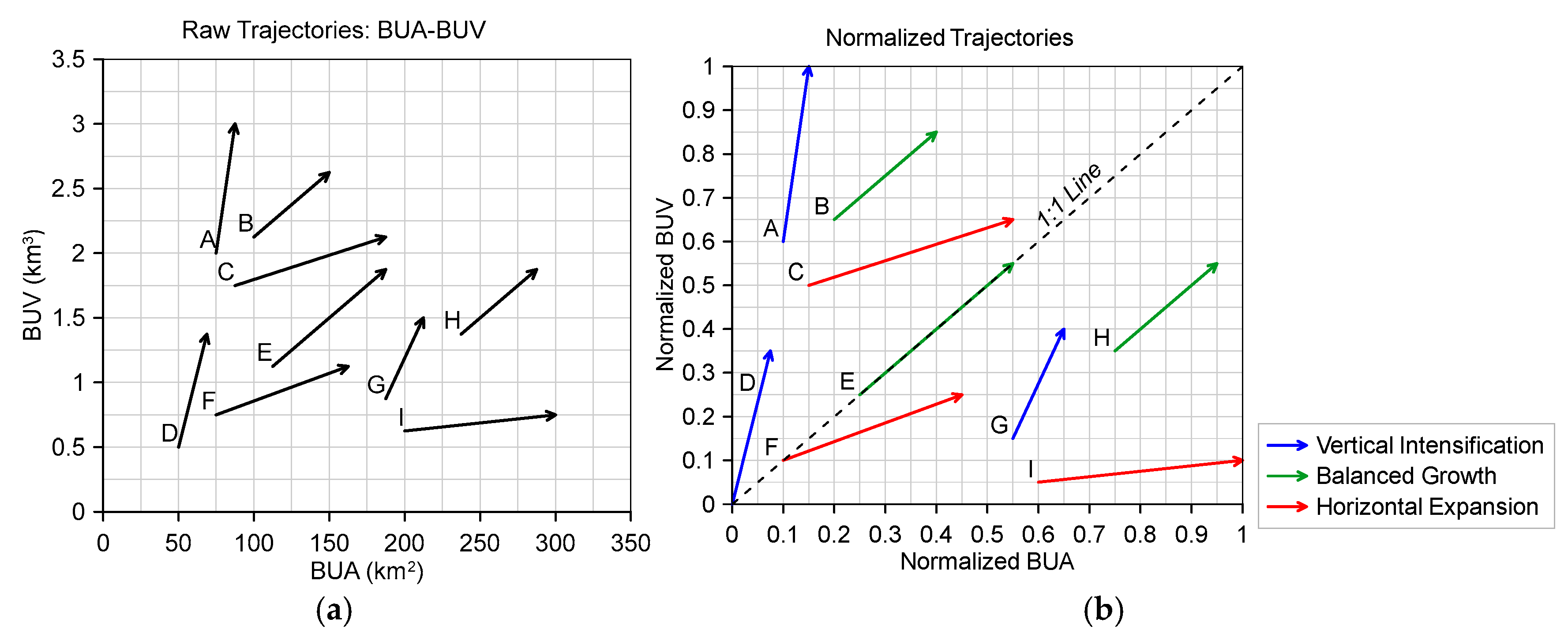
Figure 2.
Geographic distribution of the 10,856 urban centers analyzed in this study, classified by UN SDG Region. Each point represents an individual urban center in the Global Human Settlement Layer Urban Centre Database (GHS-UCDB 2025).
Figure 2.
Geographic distribution of the 10,856 urban centers analyzed in this study, classified by UN SDG Region. Each point represents an individual urban center in the Global Human Settlement Layer Urban Centre Database (GHS-UCDB 2025).
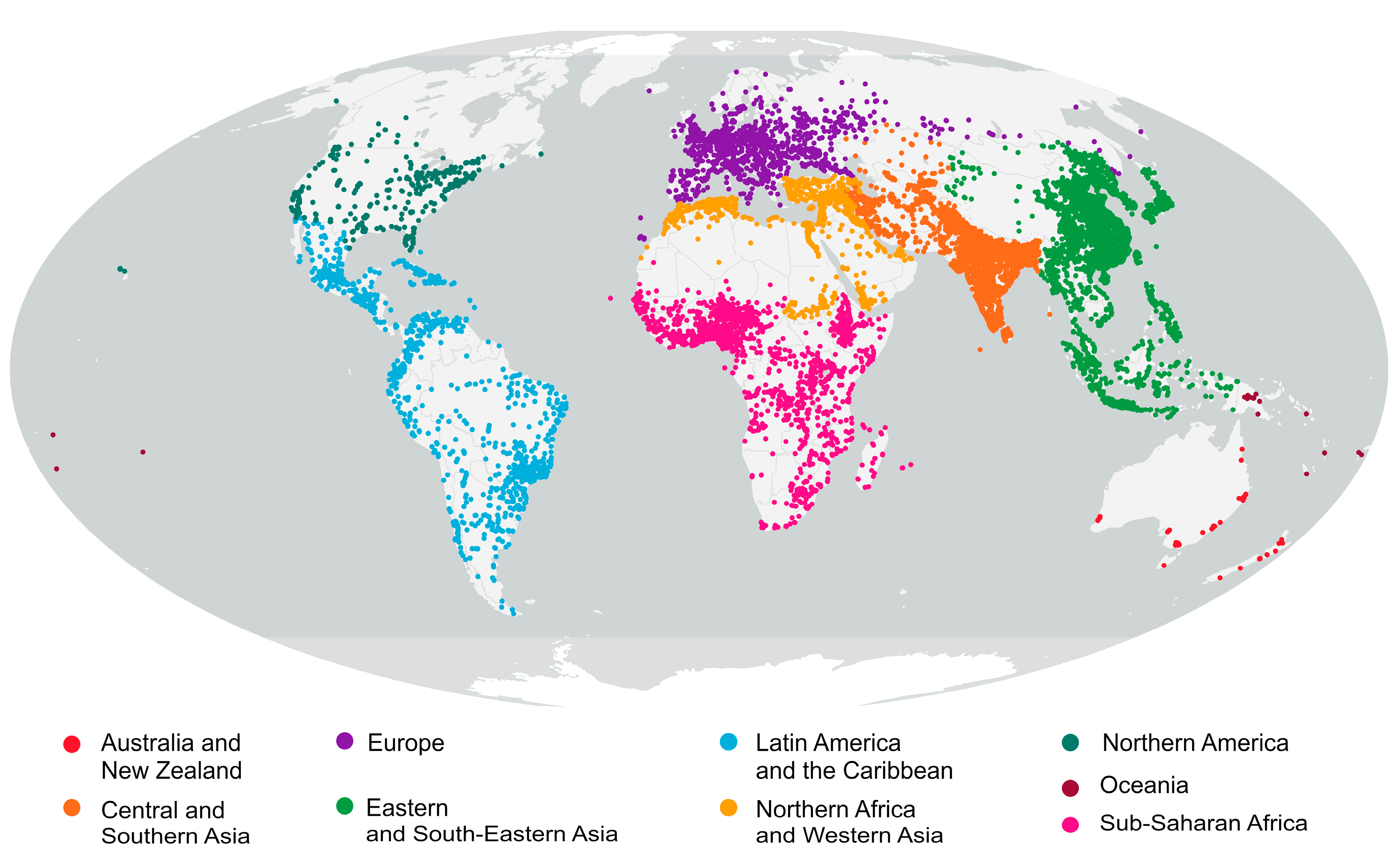
Figure 3.
Trajectories of urban centers in raw and normalized BUA–BUV space from 1980 to 2020. Panels (a) and (b) show raw and normalized trajectories, respectively, for all urban centers in the dataset. Panels (c) and (d) present the corresponding trajectories for the top 10 most populous urban centers in 2020 based on the Global Human Settlement Layer Urban Centre Database (GHS-UCDB 2025).
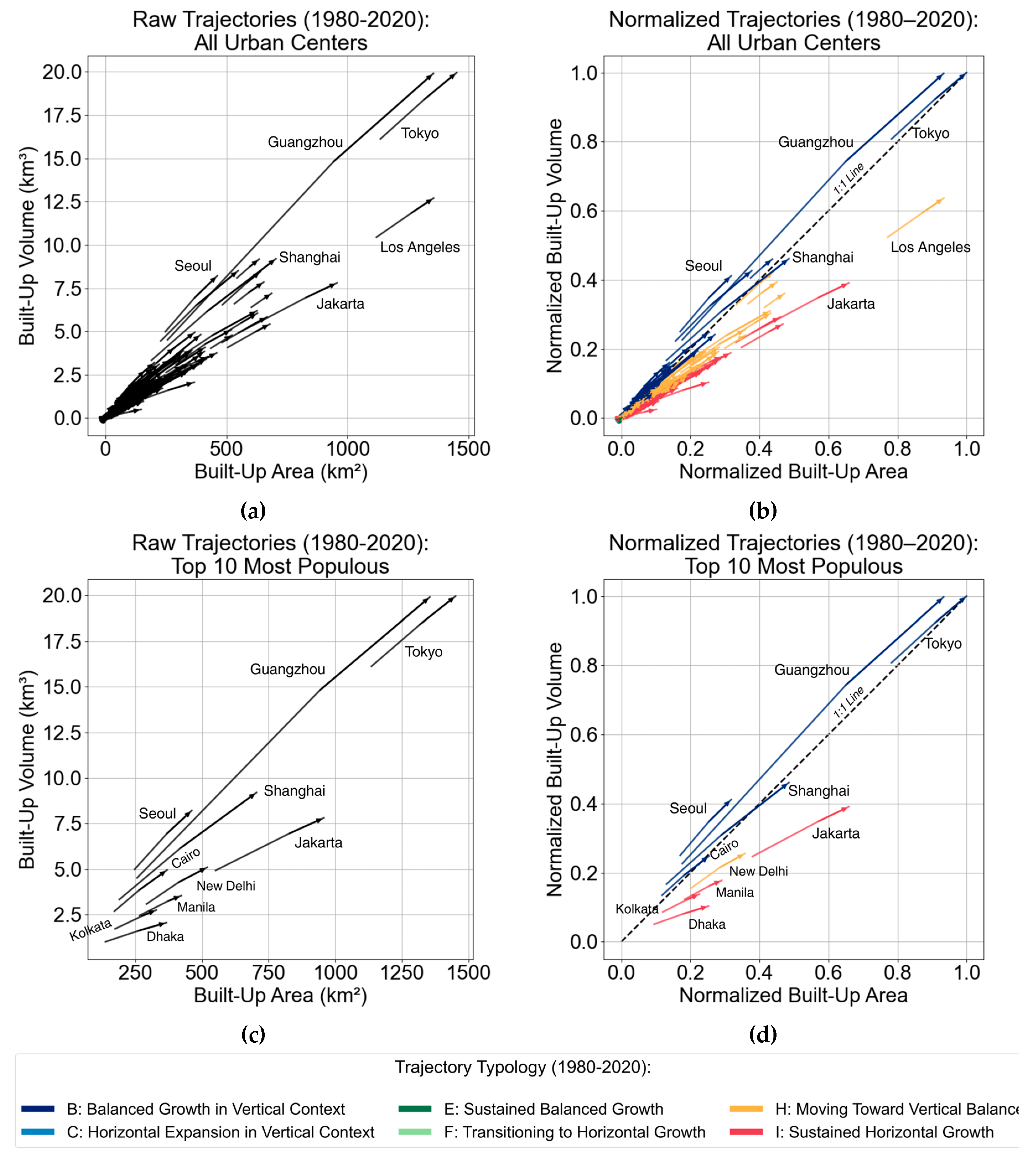
Figure 4.
Distribution of prevailing built form dominance among urban centers in 1980, 2000, and 2020 based on normalized BUA–BUV values.
Figure 4.
Distribution of prevailing built form dominance among urban centers in 1980, 2000, and 2020 based on normalized BUA–BUV values.
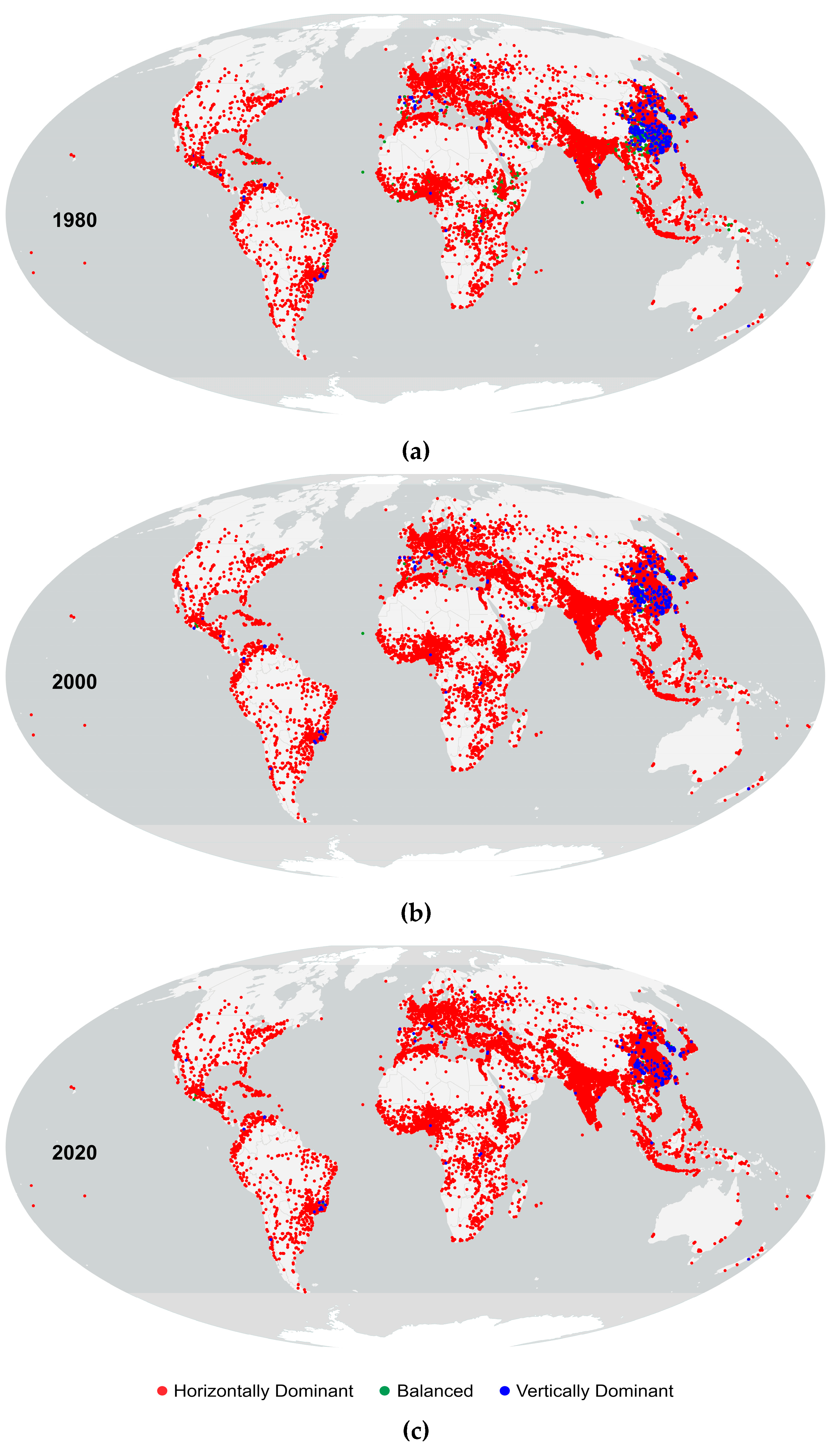
Figure 5.
Global distribution of urban centers by BUA–BUV trajectory typology for 1980–2000, 2000-2020 and 1980–2020. Each point represents one urban center classified into one of nine typologies based on prevailing built form and growth direction. For the three periods analyzed, only six of the nine typologies were observed among the urban centers.
Figure 6.
Distribution of LCRPGR values across global urban centers for the periods 1980–2000, 2000–2020, and 1980–2020.
Figure 6.
Distribution of LCRPGR values across global urban centers for the periods 1980–2000, 2000–2020, and 1980–2020.
Figure 7.
Percentage distribution of urban centers classified into three LUE classes across (a) SDG regions and (b) World Bank Income Group (WIG) for the periods 1980-2000 and 2000-2020. Urban centers not classified under any WIG were excluded from panel (b). The total number of urban centers per SDG region or income group is indicated in parentheses.
Figure 8.
Percentage distribution of urban centers across BUA–BUV trajectory typologies for three LCRPGR-based LUE classes (≤ 0, 0–1, > 1) during 1980–2000 and 2000–2020. The total number of urban centers per LUE class is indicated in parentheses.
Figure 8.
Percentage distribution of urban centers across BUA–BUV trajectory typologies for three LCRPGR-based LUE classes (≤ 0, 0–1, > 1) during 1980–2000 and 2000–2020. The total number of urban centers per LUE class is indicated in parentheses.

Table 1.
Interpretation of LCRPGR values based on the sign and relative magnitude of land consumption rate (LCR) and population growth rate (PGR), as defined under SDG 11.3.1 [1,2].
| Case | LCR | PGR | LCRPGR | Interpretation |
|---|---|---|---|---|
| 1A | > 0 | > 0 | > 1 | Land consumption exceeds population growth; indicates inefficient land use (e.g., sprawl, low-density expansion). |
| 1B | > 0 | > 0 | = 1 | Proportional land consumption and population growth; represents the ideal condition for land use efficiency, where the land consumption rate matches the population growth rate, indicating that urban expansion is aligned with demographic demand. |
| 1C | > 0 | > 0 | < 1 | Population grows faster than land expansion; denotes efficient land use, typically via densification or compact growth. |
| 2 | > 0 | < 0 | < 0 | Urban expansion amid population decline; reflects highly inefficient land use and unsustainable spatial growth. |
| 3 | < 0 | > 0 | < 0 | Built-up area contracts as population increases; may indicate efficient densification but can also lead to overcrowding if unmanaged. |
| 4A | < 0 | < 0 | < 1 | Both LCR and PGR decline; if LCR declines faster, indicates efficient urban contraction. |
| 4B | < 0 | < 0 | > 1 | Both LCR and PGR decline; if PGR declines faster, it indicates inefficient shrinkage with possible underutilization of urban space. |
| 5 (Special case) |
Any | = 0 | Undefined | PGR is zero; LCRPGR is undefined. Interpretation depends on LCR: if LCR > 0, it indicates inefficiency; if LCR < 0, it may suggest efficient contraction. |
| 6 (Special case) |
= 0 | ≠ 0 | 0 | No change in land consumption. If PGR > 0, it indicates maximum efficiency; if PGR < 0, it reflects ambiguous conditions needing contextual analysis. |
Table 2.
Typology of urban growth patterns based on the trajectory of normalized Built-up Area (BUA) and Built-up Volume (BUV), under the assumption of simultaneous increases in BUA and BUV over time.
Table 2.
Typology of urban growth patterns based on the trajectory of normalized Built-up Area (BUA) and Built-up Volume (BUV), under the assumption of simultaneous increases in BUA and BUV over time.
| Typology Name | Trajectory Starting Position | Prevailing Built-Form at Starting Position | Slope (Trajectory Angle, measured counterclockwise from the BUA axis) | Growth Mode | Interpretation |
|---|---|---|---|---|---|
| A: Vertical Intensification | Above the 1:1 Line | Vertically dominant | Steeper (60°–90°) | Vertical intensification | Growth is driven primarily by built-up volume; vertically dominant cities become more compact. |
| B: Balanced Growth in Vertical Context | Above the 1:1 Line | Vertically dominant | Moderate (30°–60°) | Balanced Growth | BUA and BUV increase at relatively balanced rates while retaining vertical dominance. |
| C: Horizontal Expansion in Vertical Context | Above the 1:1 Line | Vertically dominant | Shallower (0°–30°) | Horizontal Expansion | BUA increases more rapidly than BUV, but vertical dominance is still maintained. |
| D: Transitioning to Vertical Growth | On or Near the 1:1 Line | Balanced | Steeper (60°–90°) | Vertical intensification | Urban form shifts from balance toward increasing vertical development. |
| E: Sustained Balanced Growth | On or Near the 1:1 Line | Balanced | Moderate (30°–60°) | Balanced Growth | BUA and BUV grow proportionally; urban structure remains balanced. |
| F: Transitioning to Horizontal Growth | On or Near the 1:1 Line | Balanced | Shallower (0°–30°) | Horizontal Expansion | Urban form shifts from balance toward increasing horizontal expansion. |
| G: Vertical Rise from Horizontal Base | Below the 1:1 Line | Horizontally dominant | Steeper (60°–90°) | Vertical intensification | Cities previously dominated by BUA show increased BUV; a shift toward vertical development. |
| H: Moving Toward Vertical Balance | Below the 1:1 Line | Horizontally dominant | Moderate (30°–60°) | Balanced Growth | Both BUA and BUV grow, with vertical development catching up; movement toward balance. |
| I: Sustained Horizontal Growth | Below the 1:1 Line | Horizontally dominant | Shallower (0°–30°) | Horizontal Expansion | Horizontal expansion continues to dominate; vertical growth remains limited. |
Table 3.
Median LCR, PGR, and LCRPGR of global urban centers. Refer to Figures S3 and S4 in the Supplementary Materials for visualizations of the full distributions.
Table 3.
Median LCR, PGR, and LCRPGR of global urban centers. Refer to Figures S3 and S4 in the Supplementary Materials for visualizations of the full distributions.
| LCR (%) | PGR (%) | LCRPGR | |||||||
|---|---|---|---|---|---|---|---|---|---|
| 1980-2000 | 2000-2020 | 1980-2020 | 1980-2000 | 2000-2020 | 1980-2020 | 1980-2000 | 2000-2020 | 1980-2020 | |
| All | 3.47 | 1.72 | 3.44 | 1.97 | 0.95 | 1.52 | 1.67 | 1.05 | 1.94 |
| UN SDG Region | |||||||||
| Australia and New Zealand | 1.19 | 0.63 | 1.06 | 1.64 | 1.48 | 1.60 | 0.96 | 0.54 | 0.77 |
| Central and Southern Asia | 6.02 | 2.15 | 5.55 | 2.21 | 0.96 | 1.60 | 2.75 | 1.63 | 3.45 |
| Eastern and South-Eastern Asia | 4.19 | 2.08 | 4.31 | 1.13 | 0.42 | 0.81 | 1.64 | 1.02 | 2.03 |
| Europe | 1.22 | 0.63 | 1.00 | 0.26 | 0.10 | 0.21 | 1.66 | 0.52 | 1.48 |
| Latin America and the Caribbean | 3.01 | 1.35 | 2.70 | 2.17 | 1.23 | 1.74 | 1.41 | 1.08 | 1.65 |
| Northern Africa and Western Asia | 2.74 | 1.79 | 2.88 | 2.79 | 1.83 | 2.31 | 1.03 | 0.97 | 1.25 |
| Northern America | 1.55 | 0.65 | 1.22 | 1.52 | 1.15 | 1.42 | 1.01 | 0.58 | 0.94 |
| Oceania | 1.89 | 0.60 | 1.29 | 2.64 | 2.16 | 2.51 | 0.66 | 0.45 | 0.61 |
| Sub-Saharan Africa | 3.37 | 2.49 | 3.90 | 2.74 | 2.25 | 2.38 | 1.38 | 1.01 | 1.69 |
| World Bank Income Group | |||||||||
| Low income | 3.52 | 2.25 | 3.84 | 3.01 | 1.87 | 2.38 | 1.43 | 0.82 | 1.74 |
| Lower Middle | 4.67 | 2.09 | 4.54 | 2.37 | 1.28 | 1.87 | 2.12 | 1.32 | 2.48 |
| Upper Middle | 3.50 | 1.77 | 3.43 | 1.48 | 0.69 | 1.18 | 1.44 | 1.06 | 1.73 |
| High income | 1.30 | 0.66 | 1.10 | 0.61 | 0.53 | 0.54 | 1.24 | 0.60 | 1.29 |
Disclaimer/Publisher’s Note: The statements, opinions and data contained in all publications are solely those of the individual author(s) and contributor(s) and not of MDPI and/or the editor(s). MDPI and/or the editor(s) disclaim responsibility for any injury to people or property resulting from any ideas, methods, instructions or products referred to in the content. |
© 2025 by the authors. Licensee MDPI, Basel, Switzerland. This article is an open access article distributed under the terms and conditions of the Creative Commons Attribution (CC BY) license (http://creativecommons.org/licenses/by/4.0/).
Copyright: This open access article is published under a Creative Commons CC BY 4.0 license, which permit the free download, distribution, and reuse, provided that the author and preprint are cited in any reuse.


