
Submitted:
16 July 2025
Posted:
17 July 2025
You are already at the latest version
Abstract
In this comprehensive study, we meticulously investigated multidimensional data analysis techniques, particularly focusing on Tucker decomposition methods, spanning the period from 2000 to 2023. Our primary objective was to discern trends, advancements, and applications of these techniques across various domains of knowledge and how they have evolved over time. An extensive corpus of 265 scientific articles related to tensor decompositions, Tucker models and applications was previously reviewed. Multivariate methods such as text mining using IraMuteq software and MANOVA-Biplot were employed to visualize identified data patterns, and the analytical capability of ChatGPT 3.5 artificial intelligence was assessed to provide contextual insights and add another layer of information to the research. Our conclusions underscore the importance of blending traditional statistical approaches with natural language processing prowess to achieve a profound understanding of the data. This analysis offers a comprehensive perspective on the evolution and application of multidimensional data analysis techniques, with a special emphasis on the enduring relevance of Tucker techniques in this new millennium.
Keywords:
Tucker decomposition
; canonical biplot
; ChatGPT 3.5
; neural networks
; scientific literature review
1. Introduction
Systematic reviews are an essential tool in scientific research, allowing the collection, analysis, and synthesis of existing information in a specific field [1]. In recent years, advances in technology and artificial intelligence have introduced new approaches to perform this task more efficiently and accurately. Two innovative approaches proposed in this study are Biplot-based Text Mining and ChatGPT artificial intelligence, which offer different perspectives on extracting scientific information.
Text Mining refers to the process of using natural language processing and data mining techniques to analyze large volumes of text and extract relevant information [2]. In a systematic review, this information can be extracted from the abstracts of scientific articles published in high-impact journals. Additionally, Biplot techniques are presented as an ideal complement to enrich text analysis, as they effectively visualize the relationships between keywords and groups of documents. This facilitates the interpretation of patterns, relationships, and trends in textual data, allowing for a deeper understanding of a particular domain. Traditionally, this has been done with Correspondence Analysis (CA) by Benzecri [3], which penalizes the most frequently used words in the text corpus that may be very common; however, they may have little semantic or informative relevance.
On the other hand, ChatGPT is a form of artificial intelligence based on generative language models, such as the GPT-3.5 model, which has the ability to understand and generate text in natural language [4]. With its ability for contextual understanding and generating coherent responses, ChatGPT can be used for tasks such as classification, summarization, and analysis of scientific information.
In this article, we present our proposal on the publications related to Tucker models in this new millennium. Tucker models, named after the eminent mathematician Ledyard R. Tucker, are highly useful tools today as they are multiway data models that play a crucial role in the decomposition and understanding of complex multidimensional data [5].
Conducting a systematic literature review on these models is an extremely complex task, given the wide range of applications they have in the scientific world. Numerous researchers are dedicated to exploring and leveraging the findings provided by these models, reflecting their importance and relevance in contemporary research.
2. Tucker Models
Tucker models are a generalization of singular value decomposition (SVD) specifically designed for tensors. In this context, a tensor can be understood as a multidimensional data structure that generalizes the concept of matrices to more than two dimensions. While a matrix has rows and columns, a tensor can have multiple dimensions or modes.
Within three-way data analysis, the STATIS techniques (Structuration des Tableaux à Trois Indices de la Statistique) [6] are noteworthy. These techniques treat three-way data as tables or data matrices to obtain a two-dimensional array, thus capturing only the stable structure of the original data [7]. In contrast, Tucker models [5] analyze the entire data cube, constructing a simplified model, thereby capturing the dynamic part of the data. This ability of Tucker models to examine the complete data cube results in much more detailed and content-rich information. These models allow for the representation of a three-dimensional tensor (or higher-order tensor) as a combination of a core tensor and a set of mode matrices that capture the underlying dynamic structure of the data [8]. This hierarchical and multidimensional structure provides a more compact and meaningful representation of the data, facilitating the identification of patterns and relationships in complex datasets [9].
In the Tucker-3 model, the three-way data tensor , where , , , which we assume, without loss of generality, consists of Iindividuals, Jvariables, and Koccasions (or time points), can be approximated by the tensor using the equation
where is a tensor of residuals.
To construct the estimated tensor , the Tucker-3 decomposition seeks to find three orthogonal loading matrices , , and ; where , , and . These matrices A, B, and C correspond to the weights for individuals, variables, and occasions respectively, and the decomposition also involves a core tensor, also known as core matrix,5.
Thus, the -th element of the tensor in equation can be expressed as
The core tensor , as shown in Figure 1, is the central element of the Tucker-3 model; it represents the interaction between the three modes of the original tensor [5,8]. It resembles a three-dimensional matrix and contains the amount of variance explained by each combination of components. This tensor has dimensions , where P, Q, and R (, , ) are the number of components or latent factors required for each mode respectively, as a result of the dimensionality reduction of the tensor . In other words, the core tensor is considered a reduced version of the data tensor [10]. Moreover, the selection of the number of components of the core tensor is still a subject of study today, with various algorithms developed in this regard.
One of the first algorithms developed to estimate the number of components, by Kroonenberg and De Leeuw in 1980 [11], is the algorithm known as TUCKALS3. This algorithm, through alternating least squares fitting, aims to minimize the function
where denotes the Euclidean norm, and the matrices (also called unfolded tensors) and are obtained by concatenating the K frontal slices of the tensors and , respectively.
Later, Timmerman and Kiers in 2000 [12] proposed the well-known algorithm DIFFIT, which determines an optimal proportion of the difference in fit or sum of squares explained by the solutions of these models known as Three-Mode Principal Components Analysis (3MPCA).
The modes are essential for defining how data is organized and related in the three-dimensional tensor [13]. The three mode matrices are used to describe how dimensions are grouped within each mode and, together, determine the structure of the core tensor,14. The Tucker-3 model can be represented using matrix equations for each of its three modes as follows:
In equations (2.4), (2.5), and (2.6), the operator ⊗ is the Kronecker product [5]. Taking mode A as an example, the matrices , , and are two-way arrays of order (), (), and (), respectively, and they are the matricized versions of the tensors X, G, and E.
As shown in Figure 2, the matricization or unfolding of the tensor is obtained by concatenating the different slices, whether they are frontal for mode A, horizontal for mode B, or lateral for mode C, in order to obtain their two-way matrix versions.
The Tucker-2 models are specific variants of the Tucker-3 model [15]. In a Tucker-2 model, out of the three available modes, two are reduced, resulting in three possible configurations of Tucker-2 models; these are Tucker-2-AB, Tucker-2-AC, and Tucker-2-BC. Similarly, Kroonenberg and De Leeuw developed the TUCKALS2 algorithm to find optimal solutions with alternating least squares. For example, in the Tucker-2-AB model, mode A is reduced to P components () and mode B is reduced to Q components (). Mode C, on the other hand, is not reduced and remains with its K original slices. This same principle applies to the other modes.
From another perspective, the Tucker-1 models are also classified as specific instances of the Tucker-3 model. In a Tucker-1 model, out of the three available modes, only one is reduced. In total, three variants of Tucker-1 models are distinguished: Tucker-1-A, which involves a component analysis on two-dimensional tables for the frontal slice supermatrix; Tucker-1-B, which involves a component analysis on two-dimensional tables for the horizontal slice supermatrix; and Tucker-1-C, which corresponds to a component analysis on two-dimensional tables for the vertical slice supermatrix. The TUCKALS1 algorithm is used for these three Tucker-1 models. For example, in the Tucker-1-A model, mode A is reduced to P components (). Modes B and C are not reduced and remain with their J and K original slices, respectively.
The challenges encountered in interpreting the results of Tucker models have driven the development of new approaches based on simpler hypotheses. In 1970, Carroll and Chang [14], as well as Harshman [16], independently proposed a model to decompose three-way tables with fully interrelated modes more directly. While the former authors called it CANDECOMP (Canonical Decomposition), Harshman named it PARAFAC (Parallel Factor Analysis).
The CANDECOMP/PARAFAC (CP) model is a constrained version of the Tucker-3 model and is defined as
where the matrix is the two-dimensional version of order of the three-dimensional superidentity tensor ; that is, , with when , and otherwise. The model is uniquely defined under certain (weak) conditions, which are often met in practice. That is, the estimates of A, B, and C are unique up to an arbitrary scaling of the columns in two of the component matrices and an arbitrary simultaneous permutation of the columns in the component matrices.
These Tucker models have found applications in a wide variety of fields, from spectroscopy [17,18,19,20,21,22,23,24,25,26,27], agriculture [28,29,30,31], data mining [32], and neuroimaging [33,34,35]. Their versatility and ability to handle high-dimensional data have driven their adoption in scientific research and have contributed to a better understanding of complex phenomena [36]. Therefore, it is crucial to document and advance the development of Tucker models due to their fundamental role in contemporary and future scientific research in the new millennium.
In this article, we conduct a systematic literature review using Biplot-based Text Mining and ChatGPT 3.5 for scientific information extraction, focusing on a specific case: the search and analysis of the literature from the year 2000 to 2023 related to Tucker models. For this purpose, searches were conducted in the Scopus and Web of Science databases, obtaining a set of relevant articles. These articles were processed using a Text Mining tool, the IraMuteq software, generating a lexical table and subsequently performing a Canonical Biplot analysis. In turn, ChatGPT 3.5 was used to perform a similar classification, evaluating similarities and differences with the Biplot-based Text Mining approach, thereby adding an additional layer of information to the systematic literature review.
3. Materials and Methods
3.1. Materials
A comprehensive search for articles in high-impact journals was conducted using specific keywords: Tucker1, Tucker-1, Tucker2, Tucker-2, Tucker3, or Tucker-3. The search was performed from January 1, 2000 to December 31, 2023 in the Scopus and Web of Science (WoS) databases, specifically.
In the search conducted in Scopus, a total of 325 publications were obtained, while 302 publications were found in WoS. In total, an initial database of 627 publications was obtained, which was subjected to a screening process. For this screening, the principles established in the PRISMA 2020 statement (Preferred Reporting Items for Systematic Reviews and Meta-Analyses), which defines guidelines for the systematic review and meta-analysis of studies [37], were applied. These guidelines allowed for the evaluation of the relevance and methodological quality of the articles, ensuring the inclusion of studies that met rigorous standards.
During the inclusion and exclusion process of articles, a series of stages were carried out to ensure the relevance of the set of articles for the study. Initially, publications with missing information in critical fields such as author, year, source, title, or abstract were discarded. These fields are considered essential for the proper analysis and understanding of the articles. As a result of this filter, 22 articles were removed (16 from WoS and 6 from Scopus), leaving a total of 605 articles, of which 286 are indexed in WoS and 319 in Scopus.
Subsequently, duplicate articles were removed; that is, articles that were found in both databases. If an article is indexed in both databases, we removed those indexed in Scopus and retained those published in WoS as a priority. We identified a total of 276 duplicate articles, which were removed from Scopus, resulting in a new total database consisting of 329 articles, of which 286 are indexed in WoS and 43 in Scopus; this database no longer contains duplicate articles.
Finally, the relevance of each article to the study, focused on Tucker models, was evaluated. At this stage, the contribution of the research and its close relation to Tucker models were considered of great importance. For this purpose, a new column was created in the MsExcel document containing the data, allowing logical values of 1 to be assigned to relevant articles and 0 to those that were not. After this evaluation, 64 articles were discarded (51 from WoS and 13 from Scopus), resulting in a final set of 265 articles, of which 235 are indexed in WoS and 30 in Scopus, ready for Text Mining analysis using IraMuteq software. This screening process is summarized in Figure 3. mynode/.style= draw, rectangle, align=center, text width=3.8cm, font=, inner sep=3ex, mylabel/.style= draw, rectangle, align=center, rounded corners, font=, inner sep=2ex, fill=cyan!30, minimum height=1.3cm, arrow/.style= thick,->,>=stealth, node distance=1.0cm
The resulting database, composed of 265 publications, was used as the definitive set to conduct the study with Text Mining tools, Canonical Biplot, and ChatGPT. This analysis will allow us to evaluate the efficiency and accuracy of each technique in extracting specific scientific information about Tucker models, as well as to identify potential advantages and disadvantages of each approach.
3.2. Research Methods
3.2.1. Text Mining with IraMuteq
The statistical analysis of textual data, commonly referred to as SATD, is a methodology that combines text analysis techniques with statistical techniques to extract meaningful information and reveal patterns and trends in large volumes of textual data [38]. The primary objective of this analysis is to explore and understand the structure and content of the texts, as well as to identify relationships between words and their context [39].
In this study, SATD was used as part of the Text Mining approach to analyze the database of 265 publications related to Tucker models from the new millennium, specifically from the year 2000 to 2023. SATD was conducted using the IraMuteq software (Interface for R for Multidimensional Analysis of Texts and Questionnaires), a free software developed by Pierre Ratinaud at the LERASS Laboratory of the University of Toulouse [40]. IraMuteq software allows for multidimensional analyses of texts of various natures, including official documents, web pages, news, and open-ended survey responses [40,41], and it enables lexical analysis and the generation of a lexical frequency table of keywords used in article abstracts [42].
The analysis with IraMuteq software is based on correspondence analysis methods and hierarchical classifications, with a focus on descending hierarchical clustering [42]. This procedure, shown in Figure 4, involves reducing context units to more manageable text segments (ECUs), followed by lemmatization to reduce words to their canonical forms [40]. Then, context units (CU) are created that meet certain criteria for active and supplementary forms [40,42].
Descending hierarchical classification is performed in stages, using correspondence factor analysis and optimization of inter-class inertias to form clusters/classes of ECUs [43]. This analysis allows for the identification of textual structures in the text corpus [44,45].
Each article in the corpus is accompanied by its corresponding abstract. These abstracts provide a concise overview of the contents and context of the full article. Abstracts are a rich source of textual information that allows the software to analyze lexical and semantic patterns based on the keywords used and their relationships [46].
It is essential that the selected corpus is focused on a specific and coherent topic, in this case, Tucker models. The thematic homogeneity ensures that the lexical and semantic analyses conducted by the IraMuteq software are relevant and meaningful in the research context [47].
Once the corpus is prepared, the next step is the segmentation of the text into Elementary Context Units (ECUs). These ECUs are short text fragments, usually two or three lines, representing indivisible units of analysis [48]. Segmentation into ECUs allows the IraMuteq software to analyze and process each fragment independently, facilitating the identification of specific patterns and features in the text [49]. Before proceeding with lexical analysis, IraMuteq software performs an automatic lemmatization stage of the words [40]. Lemmatization involves reducing each word to its canonical or root lexical form [50]. This way, different forms of the same word are grouped under a single form, simplifying the analysis and ensuring greater consistency in the results obtained [51].
Once the words have been lemmatized, the IraMuteq software proceeds to create Context Units (CU) [51]. Each CU is a set of ECUs that share a certain minimum number of "active forms," which are generally verbs, nouns, adverbs, and adjectives. These active forms are relevant for lexical and semantic analysis as they contain key information about the content of the text [52].
From the CUs, the IraMuteq software constructs frequency tables, which are tables showing the frequency of occurrence of each active form in each CU [53]. These tables are crucial for correspondence analysis and identifying patterns in textual data. The IraMuteq software performs a Correspondence Factor Analysis (CFA) on these contingency tables to detect relationships and similarities between the active forms and the CUs [3].
The product we will use from the IraMuteq software analysis is a lexical table that shows the relationships between active forms (lemmatized words) and CUs [54]. In this table, each row represents a CU, and each column represents an active form. The cells of the table contain information about the frequency of occurrence of each active form in each CU [43]. The lexical table is a visual representation of the lexical and semantic relationships in the analyzed corpus, allowing for the identification of patterns and trends in textual data [52].
3.2.2. Multivariate Analysis of the Lexical Table with Canonical Biplot
The lexical table obtained from the IraMuteq software is a cross-frequency table that has traditionally been used for Benzecri’s Correspondence Factor Analysis (CFA). CFA is a multivariate technique that examines dependency relationships between categorical variables and generates profiles based on relative frequencies. In this method, the most frequent words are penalized using a weighted chi-square distance to measure relationships between categories in a contingency table. These weights are essential for calculating the weighted chi-square distance and are an integral component of the method.
However, CFA has limitations in describing the group structure of individuals and assessing significant differences between them. In these cases, Canonical Analysis is used, particularly Canonical Biplot or MANOVA Biplot, which provides a graphical representation associated with MANOVA or Discriminant Analysis. This approach offers a more comprehensive view of the group structure and the statistical significance of the differences between them [55].
Amaro et al. [55] justify the use of Canonical Biplot instead of CFA in the analysis of data with group structure. They note that, from a statistical standpoint, CFA does not consider the group structure of individuals and is not suitable for studying the significance of differences between groups. In contrast, MANOVA can be used to study the significance of differences between groups, and Canonical Analysis is used to study the dimensionality of the alternative hypothesis when the null hypothesis is rejected in MANOVA [56].
The Canonical Biplot is an extension of Canonical Analysis that combines information about group means and variables from a data matrix [55]. It allows for a joint representation of group means and variables in a two-dimensional space, where group means are projected onto the canonical variates, which are linear combinations of observed variables that best explain the differences between groups [57]. The variables are positioned on the plot in directions that best predict the actual mean values for each variable [58].
The matrix approach to the MANOVA model for n variables is defined as follows:
In this formulation, represents a matrix of dimensions , which stores the observations. The matrix , of rank t, refers to the design matrix, which is set by the researcher, while corresponds to the matrix of unknown parameters. Lastly, , a matrix of size , stores the model residuals or random deviations [58].
The MANOVA-Biplot, once the model is fitted, presents the null hypothesis, which is fundamental for testing linear hypotheses such as
where and are full-rank matrices, and their rank is [59].
The selection of the matrices and can vary, allowing for the construction of Biplots for different study hypotheses. Typically, and include a set of coefficients for making contrasts.
In the Canonical Biplot, similarities between groups are interpreted based on Mahalanobis distances; the variables responsible for differences between groups are projected onto the group directions, and correlations between variables are represented as angles between vectors on the plot [60]. Acute angles indicate positive relationships, obtuse angles indicate negative relationships, and right angles are interpreted as independence [61].
The interpretation of the canonical axes, which are linear combinations of variables derived in Canonical Component Analysis (CCA), is typically done through the correlations between the observed variables and the canonical axes, although these relationships are not maximized by the technique [55]. Instead, the use of the quality of representation of group means is proposed as a measure of result accuracy. The quality of data representation is obtained through the Quality Representation Index (QRI) [62]. This index measures the percentage of variability of group means represented by the reduced-dimension solution and corresponds to the squared cosine of the angle between the point/vector in multidimensional space and its projection in the low-dimensional solution [63]. A QRI is calculated for both group means and variables [64]. In the Canonical Biplot, it is possible to draw a confidence circle around the projection of the means for each variable. These constructed circles allow us to visually identify significant differences between groups in terms of the variables being analyzed [55].
In this study, once lexical tables were obtained from text analysis using IraMuteq software, a multivariate analysis was performed using the Canonical Biplot or MANOVA Biplot method. The main objective of this analysis was to group the articles based on their publication periods and explore trends and changes over time in relation to Tucker models.
To carry out the Canonical Biplot, the articles were divided into four groups based on six-year publication periods: group 1 (2000-2005), group 2 (2006-2011), group 3 (2012-2017), and group 4 (2018-2023). Each group represented a specific period during which Tucker models were studied, allowing for the analysis of the evolution of these models over time.
In the Canonical Biplot, the lexical tables obtained through the IraMuteq software were used to represent the groups of articles and the variables (keywords) in a two-dimensional space. The group means (represented by the articles belonging to each previously defined period) were projected onto the canonical axes, which are linear combinations of the lexical variables that best explain the differences between groups. Thus, each group was positioned in the Canonical Biplot space according to its specific lexical characteristics.
The keywords (variables) were also placed on the plot based on their relationships with the groups. The words responsible for the most significant differences between groups were projected in the directions of the corresponding groups, allowing the identification of which terms were most associated with each specific period.
Additionally, the Canonical Biplot facilitated the interpretation of similarities and differences between groups and variables. Mahalanobis distances were used to assess dissimilarities between the groups on the plot, while the angles between the keyword vectors allowed for the analysis of correlations among them.
The application of the Canonical Biplot in this study provided a clear visualization of the group structure of the articles based on their publication periods and revealed patterns and trends related to Tucker models over time. It also provided a rich and detailed graphical representation that helped better understand the relationships between the keywords and groups, facilitating a deeper interpretation of the results obtained.
3.2.3. ChatGPT for Classification
ChatGPT, developed by OpenAI, is a powerful natural language processing system powered by artificial intelligence (AI) [65]. It belongs to the GPT (Generative Pre-trained Transformer) series, which has stood out for training massive language models on large amounts of text to learn linguistic patterns and complex grammatical structures [66].
The latest known free version, GPT-3.5, also called ChatGPT, represents a milestone in the evolution of AI [67]. This model has been able to generate coherent and relevant text thanks to its architecture based on neural networks known as Transformers, which allows it to understand and generate text based on the provided context [66]. The GPT-3.5 model, like its predecessors, is characterized by its "pre-training" approach [65,68]. This means that the model is trained on large amounts of text without a specific task in mind. During the training process, the model learns linguistic patterns, semantic relationships, and general encyclopedic knowledge [69].
The Transformer architecture is notable for its self-attention mechanism and its encoder-decoder layers [70]. The self-attention mechanism allows the model to focus on relevant parts of the input text by assigning weights to different words based on their relevance to understanding the context [71]. Additionally, GPT-3.5 has a massive structure consisting of 175 billion parameters [72]. This makes it one of the largest and most powerful language models ever created, allowing it to generate highly coherent and contextually relevant text [73].
The pre-training process of ChatGPT involves presenting the model with a large amount of text collected from the web. During this process, the model tries to predict the next word or token in a given sequence, allowing it to learn the probability of occurrence of different words based on the context [74].
Once the model has been pre-trained, it can be fine-tuned for specific tasks by providing labeled examples [75]. This allows developers to tailor the model for specific tasks, such as answering questions, translating languages, generating creative text, and, as in this work, adding an additional layer of relevant information to the Systematic Literature Review [76].
It is important to note that while GPT-3.5 is a marvel of artificial intelligence, it still has limitations and challenges. For example, it can generate plausible but inaccurate responses and may be sensitive to biases present in the training data [77]. These issues are the subject of ongoing research and development to improve the model’s accuracy and fairness; in fact, at the time of this research, there are newer versions available for purchase [78].
The use of ChatGPT is diverse and ranges from virtual assistants to chatbots and text generation for various applications [79]. Users can interact with it through text commands (prompts), and the model will respond in a contextually relevant manner [79]. One of the key concepts in using ChatGPT is "prompts," or text commands used to guide text generation [78]. Prompts are instructions or questions provided to the model to direct its output based on the specific task to be performed [66]. Proper use of prompts is essential to obtaining accurate and relevant responses [79].
Optimizing the use of prompts involves carefully choosing words and grammatical structures to clearly communicate the desired task or question [72]. It may also require adding specific constraints or indications to avoid inappropriate or irrelevant responses. Iteration and experimentation with different prompts are common practices to refine the desired text generation [72].
According to [66], although language models like ChatGPT can provide valuable information and complementary analysis, it is important to keep in mind that in certain cases, the generated information may not be completely reliable. This is due to several reasons:
- Training data: Language models like ChatGPT learn from large amounts of textual data available online. If these data contain incorrect or biased information, the model may generate responses that reflect those limitations.
- Pattern-based generation: Language models do not understand context in the same way humans do. They often generate responses based on patterns present in the training data, even if the response is not coherent or accurate.
- Unverified information: Language models cannot verify the accuracy of the information they generate. They may produce statements that sound convincing but are not supported by reliable evidence.
- Bias and neutrality: Models can capture biases present in the training data and replicate them in the generated responses. This can lead to responses that reinforce biases or stereotypes.
To mitigate these issues, it is crucial to properly train and fine-tune language models before using them for specific tasks [77]. This involves providing relevant and correct examples and guiding the model toward generating accurate and reliable responses [78]. It is also essential to cross-check the results generated by the AI tool with information from reliable sources and experts in the field [79]. When using artificial intelligence as a support tool, it is necessary to exercise critical judgment and verify the consistency and accuracy of the generated information to ensure the integrity of analyses and results [75].
It is important to highlight that the use of language models like ChatGPT for text analysis complements traditional techniques such as those used with IraMuteq software and allows for more robust and detailed results, especially in large datasets and in research that requires a more sophisticated and automated approach. However, it is also important to note that these language models should be used with caution and that the results obtained should be validated through additional analyses and expert review in the field of study.
4. Results
4.1. Data Preparation for Text Mining
To generate the data matrix used in the analysis, certain methodological adjustments were made. First, articles were obtained from the prestigious academic databases Scopus and Web of Science. These articles were selected focusing on the fundamental fields for our study, including the author’s name, the year of publication, the source of publication, the title of the article, and, most importantly, the abstract. It is important to note that the text mining analysis will be based on the latter field, as it provides a concise but informative summary of the article’s content.
Following the methodological guidelines established by Caballero et al. [80], a lexical table was constructed using a specific approach. A plain text file was created that includes a unique identifier for each article, accompanied by its respective abstract. It is crucial to mention that, in this context, it is pertinent to perform additional cleaning of the abstracts. Occasionally, some journals add copyright clauses at the end of the abstracts that are not the focus of the text mining analysis. Therefore, it is recommended to exclude this content to ensure the integrity and homogeneity of the analysis.
Additionally, it has been observed that the IraMuteq software tends to omit the first abstract during the analysis. To address this issue, it is suggested to duplicate the first abstract in the plain text file. This measure ensures that the analysis with IraMuteq software is conducted completely and accurately, without losing valuable information that may be contained in the first abstract of the selected articles.
4.2. Results of Text Mining
Once the textual corpus under study was loaded into the IraMuteq software, we present the results obtained, starting with the similarity analysis, based on graph theory. A graph, in this context, represents a set of vertices (which correspond to words or forms) and edges (which represent the relationships between them). The purpose of this analysis is to investigate the proximity and relationships between the elements of a set, optimizing the simplification of the number of connections until a connected acyclic graph is obtained. This is characterized by being a closed path in which no vertex is repeated, except for the first one, which acts as both the start and end of the path, as illustrated in Figure 5.
As can be seen, to obtain the graph shown, some adjustments were made in the IraMuteq software, considering words that, in addition to having high frequencies, are connected to the topic in question, the Tucker models. In the similarity graph, three clusters are observed, represented by different colors. Within these clusters, there are larger words (called the maximum tree of each cluster that interconnects them: "model", "datum," and "tucker3"). At the same time, within each cluster, these higher-frequency words are connected to other words that had strong connections in the textual corpus.
In the central cluster, we have the term "model," which acts as the central or most prominent node. Within this cluster, some terms are strongly connected, such as: "factor," "tucker," "tucker2," "function," and "core"; this suggests the presence of factorial analysis and mathematical functions for Tucker models, particularly Tucker-2, where the core tensor, also known as the core matrix, is involved.
In the left cluster, we identified the term "tucker3," which acts as the maximum tree and is strongly associated with other words such as: "parafac," "parafac2," "decomposition," "sdv," "tensor," "tucker1," "candecomp," "orthogonal," and "factorization." For example, "parafac" and "parafac2" refer to variants or extensions of the PARAFAC model, while "decomposition" indicates tensor decomposition. On the other hand, "Candecomp" refers to CANDECOMP/PARAFAC decomposition and also indicates the orthogonality property associated with certain decomposition methods.
The third cluster, located on the right, has "datum" as the maximum tree, which is connected to a series of keywords such as: "method," "analysis," "component," "transform," "functional," "cluster," "multiway," "computational," "matrix," "mode," and "algorithm." This structure suggests a variety of related concepts and terms. For example, it indicates different approaches or methods for data analysis, which are related to decomposing data into simpler components and data transformation for various analysis purposes, including cluster analysis.
4.3. Data Preparation for MANOVA-Biplot
One of the primary functions of IraMuteq software lies in its ability to generate a lexical table or matrix called tableafmc, which can later be subjected to Correspondence Factor Analysis (CFA) as proposed by Benzecri [3], a statistical technique used to analyze contingency tables to explore relationships between the categories of two categorical variables. In the context of textual analysis, this table shown in Table 1 incorporates the identifiers assigned to each article as variables and the words identified from the analyzed corpus as rows.
The lexical table is a fundamental representation that allows us to analyze and understand the frequency of keywords in the corpus of articles related to Tucker models. Through this table, the distribution of words and their relevance in each publication period can be visualized.
Constructing the lexical table involved transforming the corpus of articles into a matrix where the rows represent the articles and the columns represent the unique words present in the corpus. For each cell in the matrix, a numerical value is assigned indicating the frequency of the word’s appearance in the corresponding article. This process provides a quantitative view of the most relevant words in the dataset.
Using the IraMuteq software, we were able to analyze this lexical table and generate a visual representation of the distribution of keywords across different publication periods. Lexical analysis techniques, such as Correspondence Factor Analysis, allowed us to identify patterns and trends in keyword frequency over time.
Following the recommendations of Caballero et al. [80], a characterization factor was applied using the formula:
where represents the frequency of a word located in row i and column j in the tableafmc matrix. This transformation aims to simplify the matrix and enhance subsequent analysis.
To perform this characterization, the integrated development environment RStudio,81 was used, where the tableafmc matrix was initially transposed and the characterization formula applied. The result was saved in a new file called data, which was stored in Excel format. To further enrich the dataset, a column indicating the publication year corresponding to each article in the original database was added. This step can be easily performed using the filters available in the software, as shown in part in Table 2.
Furthermore, for conducting a group study following the MANOVA-Biplot approach, an additional column numbered from 1 to 4 was added to the data file, indicating the group to which each article belongs. This classification is based on a date table specifying the publication time intervals, where each number represents a different period, as shown in Table 3.
4.4. Results of the MANOVA-Biplot
Once the groups corresponding to the publication periods of the articles were defined, in our case, we have 4 groups, each spanning 6 years according to Table 3, chosen to maintain homogeneity concerning the number of years analyzed. We then proceeded to load the database called data into the MultBiplot software [82] version 18.0312, a tool developed in the Department of Statistics at the University of Salamanca, widely used in multivariate data analysis. In this context, the software allows for the import of data from Excel and the definition of the group variable as nominal, along with the specification of the 4 categories corresponding to that variable. Subsequently, we performed the one-way MANOVA-Biplot analysis.
After running the analysis in the software, we made various modifications to adjust and improve data visualization, thus obtaining a more accurate representation, as shown in Figure 6. In this regard, advanced visualization techniques were implemented, including Voronoi regions and confidence circles. These regions, named after the Russian mathematician Georgy Voronoi, are used to delimit areas on a plane based on proximity to a given set of points, allowing for better interpretation and understanding of the groups identified in the analysis [83]. On the other hand, the confidence circles shown highlight the significant differences between the means since they do not intersect.
Table 4 details how the main dimensions capture variability in the data. The first dimension or first canonical variable has an eigenvalue of 20.49 and an explained variance of 46.28%, meaning it explains 46.28% of the variability between groups. This dominant factor captures nearly half of the variability between groups, while the second component explains 31.61%; in other words, the first two canonical variables explain 77.89% of the total variability, suggesting a deep understanding of the data structure. Additionally, the p-values associated with the canonical variables are nearly zero, indicating high statistical significance and confirming the robustness of the model. This detailed evaluation provides a comprehensive view of the underlying relationships between the two sets of variables, thus supporting the validity and reliability of the analysis.
The results in Table 5, Quality of representation of group means, show how the different year groups are represented on the axes of the canonical biplot analysis. Each group corresponds to a specific period (e.g., "2000-2005", "2006-2011", etc.), and the values in the "Axis 1" and "Axis 2" columns represent the coordinates of that group on the two main axes of the Biplot; additionally, we multiplied their original values by 1000 and added an accumulated quality column to facilitate interpretation.
Groups 3 and 4, i.e., the years 2012-2017 and 2018-2023, present the highest qualities of representation on the first two factorial axes (1000 and 988, respectively), followed by group 1 (549) and finally group 2 (435) with relatively low quality compared to the other groups. This suggests considering that this group will be better represented on axes 2 and 3. However, in general terms, we have a very good quality representation of the canonical groups on the first two axes.
Next, the graph of the Canonical Biplot analysis is presented, visualizing the relationships between groups corresponding to different year periods. Each group is represented in the Biplot by a set of coordinates on the main axes. This analysis allows us to observe the trends and patterns in the evolution of keywords over time concerning Tucker models.
Focusing on the result of the MANOVA-Biplot analysis obtained in Figure 6, four regions representing the publication periods of the articles are identified: "2000-2005", "2006-2011", "2012-2017", and "2018-2023". A notable feature is the significant increase in the number of keywords as we move forward in time. This suggests an expansion in the scope and focus of research, with diversification in the thematic areas addressed concerning Tucker models.
It is also observed that there are many similarities between the groups of articles from the periods 2000-2005 and 2006-2011 (groups 1 and 2) since they are very close on the graph; on the other hand, groups 3 and 4 are far from the others, suggesting that the topics covered in those periods are significantly different but within the scope of Tucker models.
In the period "2000-2005," the inclusion of the terms "hiclas" and "binary" suggests a focus on data organization and hierarchy, which corresponds to hierarchical classes of binary data through Tucker models. This indicates the exploration of complex structures and relationships between variables. The appearance of "Candecomp" refers to CANDECOMP (CANonical DECOMPosition); in addition, terms such as "Tucker3," "PCA," and "PARAFAC," which are fundamental techniques in Tucker models, are included. Their inclusion in this period indicates continued interest in researching and developing these techniques in the early years of this millennium, although they are models developed in the last century.
The inclusion of terms such as "pollution," "chemical," "chemometric," "water," and "contamination" suggests a focus on applying Tucker models in contexts related to the assessment and modeling of pollution and water quality. This indicates an interest in analyzing environmental and health-related data during that period.
In group 2, period "2006-2011," the repeated presence of terms such as "dimensionality" and "transform" indicates a concentration on generating and transforming data using Tucker models during this period. These terms suggest a focus on the manipulation and conversion of data into useful and analyzable formats.
The presence of the term "fuzzy" indicates a focus on studying Tucker models with imprecise or fuzzy data. Taken together, these findings suggest an emphasis on innovation and advancement in tensor analysis during this specific period, highlighting the importance of exploring and understanding the complexities of Tucker models to address challenges in various application areas.
During the period 2012-2017, the published articles present a varied focus covering different aspects of the research. There is an interest in updating methods and techniques, such as "sparse." Additionally, the term "cd" suggests an interest in studying Tucker models for compositional data.
There is also an evident focus on data visualization ("visualization") and dimension estimation ("dimension"), which suggests an emphasis on understanding and visually representing information; these terms also suggest the study of the number of components or dimensions to retain for each mode in Tucker models. The presence of terms like "dna," "efficiency," "diagnostic," "fluorescence," "mine," "ecological," and "denoising" indicates a diversity of application areas, ranging from environmental research to molecular biology. These terms reveal multidisciplinary and multifaceted research during this period, covering everything from the refinement of analytical techniques to the application of tensor analysis in various fields of study.
Finally, in the group corresponding to the period "2018-2023," there is a concentration of keywords such as "robust," "highly," "algorithm," "multidimensional," "massive," "network," "numerical," "mimo," and "communication." These keywords reflect a technically and conceptually advanced landscape concerning Tucker models in the most recent period. There is a focus on areas such as advanced algorithms, image processing, computational efficiency, pattern recognition, and neural network applications in communication, among others.
The knowledge development line in Tucker models has evolved from their fundamental development to their application in complex and dynamic problems across various fields. Over the years, a deeper understanding of Tucker models and their integration with other analytical methods has been achieved, leading to significant advances in multidimensional data analysis and understanding patterns and trends over time. Up to this point in the study, we have conducted a traditional, subjective, and superficial interpretation of the scientific contributions of the new millennium within the context of Tucker models. In this sense, it is essential to add an additional layer of information using artificial intelligence.
4.5. How Can AI Enhance the Results of Text Mining?
Artificial intelligence, specifically ChatGPT 3.5, enhances text mining on article abstracts related to Tucker models by offering a deep interpretation of the context, generating additional summaries that highlight key points, identifying emerging trends and patterns, providing practical examples of application, and analyzing fundamental opinions. This facilitates a more comprehensive understanding of research in this field and guides future research areas with greater clarity and precision.
To maximize the effectiveness of ChatGPT 3.5 in text mining for Tucker models, it is crucial to design well-structured prompts that ensure accuracy, coherence, and relevance in the generated responses. The way a prompt is formulated significantly influences the quality of insights derived from the AI model. Table 6 presents key strategies for optimizing prompt design, including specificity, step-by-step structuring, the use of examples and constraints, iterative refinement, and bias control. Implementing these strategies enhances the precision of text analysis, reduces irrelevant information, and allows for a more structured extraction of meaningful patterns from the literature.
To conduct this study, we accessed the OpenAI website (www.chat.openai.com) and used the ChatGPT version 3.5 platform. It is recommended that users first create an account on the platform to establish the proper use of artificial intelligence. Then, we entered the initial prompt while maintaining the structure shown in Table 7.
With this set of instructions to ChatGPT, capturing the main findings of each article is ensured. As shown in Figure 7, ChatGPT is initially prepared to receive the information from the corresponding articles for each group. Specifying the format of the provided data is important to subsequently create a timeline to capture the main findings detected. Additionally, due to the processing limitations of this free version of ChatGPT 3.5, the dataset to be entered was divided into groups of no more than 20 articles per entry until the total was reached.
Once the abstracts were entered, the artificial intelligence identifies the main findings. These results are then compared with the information captured in the MANOVA-Biplot analysis. This multi-layered validation ensures consistency, highlights key patterns, and identifies potential discrepancies between AI-generated insights and traditional statistical approaches. This process is crucial because ChatGPT can generate erroneous results, potentially biased by the user’s prior information, query region, language, and other factors.
4.6. ChatGPT 3.5 Results for Textual Analysis of Articles Related to Tucker Models in the Period 2000-2023.
The following results correspond to the year-by-year outputs generated by ChatGPT 3.5 throughout the study period.
 Here are the main findings of the articles grouped by year:
2000: Louwerse and Smilde extended the theory of batch process MSPC control charts and developed improved control charts based on Unfold-PCA, PARAFAC, and Tucker3 models. They compared the performance of these charts for different types of faults in batch processes. Timmerman and Kiers proposed the DIFFIT method to indicate the optimal number of components in trilinear principal component analysis (3MPCA). This method outperformed others in simulations by correctly indicating the number of components.
2001: Gurden et al. presented a "grey" model that combines known and unknown information about a chemical system using a Tucker3 model. This was illustrated with data from a batch chemical reaction. Bro et al. highlighted the fundamental differences between PARAFAC and Tucker3 models and proposed a modification of the multilinear partial least squares regression model. Simeonov et al. applied multivariate statistical methods to drinking water data, highlighting water quality in different systems. De Juan and Tauler compared three-dimensional resolution methods of chemical data and suggested that Tucker3 and MCR-ALS are suitable for non-trilinear data. Estienne et al. used the Tucker3 model to extract useful information from a complex EEG dataset, identifying irrelevant sources of variation.
2002: Gemperline et al. used Tucker3 models to analyze multidimensional data from fish caught during spawning, identifying migratory patterns. Amaya and Pacheco described the Tucker3 method for three-way data analysis and its practical application. Lopes and Menezes compared the PARAFAC and Tucker3 models for industrial process control. Smoliński and Walczak developed a strategy to explore contaminated datasets with missing elements using robust PLS and the expectation-maximization algorithm. Pravdova et al. showed how N-way PCA can improve the interpretation of complex data, using Parafac and Tucker3 models.
2003: Huang et al. provided an overview of multi-way methods in image analysis, highlighting the application of PARAFAC and Tucker3 models in image analysis. De Belie et al. investigated sound emission patterns when chewing different types of dry and crunchy snacks, using multivariate analysis to distinguish between snack groups. Bro and Kiers proposed a new diagnostic called CORCONDIA to determine the appropriate number of components in multiway models. Kiers and Der Kinderen presented an alternative procedure for choosing the number of components in Tucker3 analysis, which was faster than existing methods. Ceulemans and Van Mechelen presented uniqueness theorems for hierarchical class models, comparing them to N-way principal component models.
2004: Muti and Bourennane developed an optimal method for lower-rank tensor approximation applied to multidimensional signal processing. Ceulemans, Van Mechelen, and Leenen introduced the Tucker3-HICLAS model for three-way trinary data, with application to hostility data. Flåten et al. proposed a method to assess environmental stress on the seabed using Tucker3 analysis on data collected in industrial pollution studies. Stanimirova et al. compared the STATIS method with Tucker3 and PARAFAC2 for exploring three-way environmental data.
2005: Kiers presented methods for calculating confidence intervals for CP and Tucker3 analysis results. Dyrby et al. applied the Tucker3 model to nuclear magnetic resonance time data, showing its usefulness in analyzing metabolic response to toxins. Wickremasinghe W.N. reviewed exploratory and confirmatory approaches for analyzing three-way data, focusing on Tucker3 analysis. García-Díaz J.C.; Prats-Montalbán J.M. characterized different soil types corresponding to citrus and rice using a Tucker3 model. Alves M.R.; Oliveira M.B. analyzed potato chips using a common load Tucker-1 model and predictive biplots. Acar E.; Çamtepe S.A.; Krishnamoorthy M.S.; Yener B. extended N-way data analysis techniques to multidimensional flow data, such as Internet chat room communication data. Kroonenberg P.M. provided an overview of model selection procedures in three-way models, particularly the Tucker2 model, the Tucker3 model, and the Parafac model. Ceulemans E.; Van Mechelen I. discussed hierarchical models for three-way binary data and proposed model selection strategies. Stanimirova I.; Simeonov V. modeled a four-way environmental dataset using PARAFAC and Tucker models to analyze air quality in industrial regions. Pasamontes A.; Garcia-Vallve S. used a multiway method called Tucker3 to analyze the amino acid composition in proteins of 62 archaea and bacteria.
2006: Jørgensen R.N.; Hansen P.M.; Bro R. investigated the use of repeated multispectral measurements and three-way component analysis to interpret measurements in winter wheat. Giordani P. addressed the problem of data reduction for fuzzy data using component models based on PCA and generalizations of three-way PCA. Ceulemans E.; Kiers H.A.L. proposed a numerical model selection heuristic for three-way principal component models. Singh K.P.; Malik A.; Singh V.K.; Sinha S. analyzed a dataset of soils irrigated with wastewater using two-way and three-way PCA models to assess soil contamination. Pasamontes A.; Garcia-Vallve S. used a multiway method called Tucker3 to analyze the amino acid composition in proteins of 62 archaea and bacteria. Acar E.; Bingöl C.A.; Bingöl H.; Yener B. compared linear, nonlinear, and multilinear data analysis techniques to locate the epileptic focus in EEG. Singh K.P.; Malik A.; Singh V.K.; Basant N.; Sinha S. analyzed the water quality of an alluvial river using four-way data models to extract hidden information. Dahl T.; Næs T. presented tools to analyze relationships between and within multiple data matrices, combining existing methods such as GCA and Tucker-1. Kiers H.A.L. discussed procedures to estimate compensating terms in three-way models before component analysis. Chiang L.H.; Leardi R.; Pell R.J.; Seasholtz M.B. compared the effectiveness of different methods for analyzing batch process data. Mitzscherling M.; Becker T. presented a new measurement system using Tucker3 decomposition to evaluate the quality of malt used. Cocchi M.; Durante C.; Grandi M.; Lambertini P.; Manzini D.; Marchetti A. used a three-way data analysis method (Tucker3) to investigate the evolution of components in Modena balsamic vinegar.
2007: Vichi M.; Rocci R.; Kiers H.A.L. discussed techniques for clustering units and reducing factorial dimensionality of variables and occasions in a three-way dataset. Singh and collaborators conducted a three-dimensional analysis of data obtained from riverbed sediments using multivariate component analysis. The Tucker3 model allowed for a joint interpretation of heavy metal distribution, element fractions, and particle sizes. Peré-Trepat and collaborators compared different multivariate data analysis methods on a three-dimensional dataset comprising 11 metal ions in fish, sediment, and water samples. Singh and collaborators analyzed the hydrochemistry of groundwater in the Indo-Gangetic alluvial plains using three-dimensional component analysis. The Tucker3 model revealed spatial and temporal variation in groundwater composition.
2008: Yener and collaborators described a trilinear analysis method for large datasets using a modification of the PARAFAC-ALS algorithm. Bandara and Wickremasinghe presented an approach for trilinear interaction analysis in trilinear experiments using Tucker3 analysis. Cocchi and collaborators monitored the evolution of volatile organic compounds from aged vinegar samples using trilinear data analysis. Hedegaard and Hassing proposed a new application of Raman scattering spectroscopy for multivariate classification problems, using trilinear data obtained from Raman spectra. Acar and Bro developed a clustering method in trilinear arrays for exploratory data visualization and identifying reasons for particular groups. Pardo and collaborators applied principal component analysis methods to two three-dimensional datasets to evaluate soil chemical fractionation patterns around a coal-fired power plant. Singh and collaborators used a trilinear model to analyze soil contamination in an industrial area and assess contaminant accumulation and mobility routes in soil profiles. Joyeux and collaborators adapted a PARAFAC-based method to denoise multidimensional images.
2009: Ceulemans and Kiers proposed model selection heuristics for choosing between Parafac and Tucker3 solutions of different complexities for three-dimensional datasets. Kopriva and Cichocki applied non-negative tensor factorization based on -divergence to the blind decomposition of multispectral images. Guebel and collaborators presented a procedure to discriminate between different operational response mechanisms in Escherichia coli using multivariate analysis. Tendeiro and Ten Berge investigated three-dimensional analysis methods such as three-dimensional PCA and Candecomp/Parafac. He Z. and Cichocki A. proposed a model selection approach for Tucker3 analysis based on PCA. Peng W. established a connection between NMF and PLSA in multi-dimensional data. Stegeman A. and De Almeida A.L.F. derived uniqueness conditions for a constrained version of parallel factor decomposition (Parafac). Oros G. and Cserháti T. demonstrated the antimicrobial effect of benzimidazolium salts using the Tucker model combined with cluster analysis. Dahl T. and Naes T. proposed a method to detect atypical assessors in descriptive sensory analysis. Bourennane S. et al. adapted multilinear algebra tools for aerial image simulation. Kopriva I. formulated a blind image deconvolution via 3D tensor factorization. Tsakovski S. et al. applied Tucker3 modeling to sediment monitoring data to assess contamination in a coastal lagoon. de Almeida A.L.F. et al. presented a restricted Tucker-3 model for blind beamforming.
2010: Giordani P. developed strategies to summarize imprecise data in a Tucker3 and CANDECOMP/PARAFAC model. Komsta L. et al. investigated retention in thin-layer chromatography and its analysis using PARAFAC. Kopriva I. used Higher-Order Orthogonal Iteration (HOOI) for spatially variant deconvolution of blurred images. Dong J.-D. et al. analyzed water quality in Sanya Bay using three-way principal component analysis. Astel A. et al. modeled three-way environmental data using the Tucker3 algorithm. Rocci R. and Giordani P. investigated the degeneration of the CANDECOMP/PARAFAC model and proposed solutions using the Tucker3 model. Kopriva I. and Cichocki A. applied non-negative tensor factorization to the decomposition of MRI images. Latchoumane C.-F.V. et al. used multidimensional tensor decomposition to extract discriminative features from EEGs in Alzheimer’s disease. Kopriva I. and Peršin A. proposed blind decomposition of multispectral images for tumor demarcation. Marticorena M. et al. characterized native maize populations using three-way principal component analysis. Favier G. and Bouilloc T. proposed a deterministic tensor approach for joint channel and symbol estimation in CDMA MIMO communication systems. de Araújo L.B. et al. proposed a systematic approach for studying and interpreting phenotypic stability and adaptability. Reis M.M. et al. applied a Tucker-3 model to environmental data, identifying evaporation and biodegradation processes. Kompany-Zareh M. and Van Den Berg F. presented a standardization algorithm based on Tucker-3 models for calibration transfer between Raman spectrometers.
2011: Oliveira M. and Gama J. proposed a strategy to visualize the evolution of dynamic social networks using Tucker decomposition. Durante C. et al. extended the SIMCA method to three-way arrays and applied it to food authentication. Kroonenberg P.M. and ten Berge J.M.F. investigated the similarities and differences between Tucker-3 and Parafac models. Wang H. et al. proposed a new Tucker-3 based factorization for feature extraction from large-scale tensors. Cordella C.B.Y. et al. used the Tucker-3 algorithm to analyze the relationship between chemical composition and sensory attributes of wheat noodles. Peng W. and Li T. studied the relationships between NMF and PLSA in multidimensional data, developing a hybrid method. Liu X. et al. presented a hybrid clustering method based on the Tucker-2 model for analyzing scientific publications. Kopriva I. et al. introduced a tensor decomposition approach for feature extraction from one-dimensional data. Unkel S. et al. proposed an ICA approach for three-dimensional data, applying it to atmospheric data. Russolillo M. et al. developed a multidimensional data analysis approach for the Lee-Carter model of mortality trends. Adachi K. presented a method for designing multivariate stimulus-response using an extended Tucker-2 component model. Cid F.D. et al. investigated temporal and spatial patterns of water quality in a reservoir using chemometric techniques. Phan A.H. and Cichocki A. proposed an algorithm for non-negative Tucker decomposition and applied it to high-dimensional data. Daszykowski M. and Walczak B. presented approaches for exploratory analysis of two-dimensional chromatographic signals. Lillhonga T. and Geladi P. used three-way methods to monitor composting batches over time, comparing them to traditional methods.
2012: Kroonenberg P.M. and van Ginkel J.R. proposed a Tucker-2 analysis procedure for three-way data with missing observations. Cordella et al. studied the degradation process of edible oils using nuclear magnetic resonance (NMR) spectroscopy. They used both a classical kinetic approach and a multivariate approach to characterize the thermal stability of the oils. Györey et al. established a flavor language for table margarines and compared two sample presentation protocols for expert panels, finding better performance with the side-by-side protocol. Gomes et al. presented a systematization of complex data structures for process and product analysis, proposing a flexible framework to handle such challenging information sources. Favier et al. proposed a deterministic tensor approach for joint channel and symbol estimation in CDMA communication systems. Akhlaghi et al. investigated DNA hybridization using gold nanoparticles and chemometric analysis techniques to study interactions of oligonucleotides from the HIV genome. Khayamian et al. proposed a second-order calibration method, Tucker 3, for ion mobility spectrometry data. Gredilla et al. compared various multivariate methods for pattern recognition in environmental datasets, concluding that PCA is suitable for general interpretation. Liu et al. proposed a new method to reduce noise in hyperspectral images using multidimensional Wiener filtering based on Tucker 3 decomposition. Soares et al. used statistical designs to extract substances from Erythrina speciosa leaves and analyzed the extracts using multivariate analysis methods. Prieto et al. applied the Tucker 3 method to evaluate the performance of an electronic nose in monitoring the aging of red wines. Ulbrich et al. analyzed data on organic aerosol composition in Mexico using 3D factorization models, identifying several types of aerosols and their size distributions. Gao et al. conducted a risk assessment of heavy metals in soils of mining areas, using the Tucker 3 model to assess contamination and ecological risk. Calsbeek presented a method to compare non-parametric fitness surfaces over time or space using Tucker 3 tensor decomposition. De Araújo et al. proposed a method to study and interpret a variable response in relation to three factors using the Tucker 3 model. Stegeman addressed problems with CP decomposition by fitting constrained Tucker 3 models for chemical equilibrium data. Liu et al. proposed a denoising method for hyperspectral images based on PARAFAC decomposition. Kompany-Zareh et al. extended the core consistency diagnostic to constrained Tucker 3 models to validate the dimensionality and core pattern. Gallo provided convenient symbols to define the sample space for different composition vectors that can be organized into a three-dimensional matrix. Baum et al. used chemometric methods to quantify the enzymatic activity of pectolytic enzymes, highlighting the effectiveness of the Tucker 3 model compared to other methods. Liu et al. presented a sparse component analysis method based on non-negative Tucker 3 decomposition to improve the dispersion of original diagnostic signals.
2013: Wang and Xu proposed a sparse component analysis method based on non-negative Tucker 3 decomposition to improve the dispersion of original diagnostic signals. Gallo M., Buccianti A. used a particular version of the Tucker model to analyze water samples collected from the Arno River in Italy, evaluating the method’s effectiveness. De Roover K. et al. demonstrated that component methods for three-way data can capture interesting structural information in the data without strictly imposing certain assumptions. Amigo J.M., Marini F. provided an overview of the main multiway methods used for data decomposition, calibration, and pattern recognition. Wang H., Xu F. et al. investigated non-negative Tucker3 decomposition methods for feature extraction from images. Attila G. et al. evaluated the reliability of sensory panels assessing beer samples using multivariate techniques. Gallo M., Simonacci V. presented the theory behind the Tucker3 model in compositional data and described the TUCKALS3 algorithm. Pardo R. et al. determined the chemical fractionation patterns of metals in waste generated during the optimization of a reactor for the removal of metals from wastewater. Bro R., Leardi R., Johnsen L.G. developed a method to correct sign indeterminacy in bilinear and multilinear models. Erdos D., Miettinen P. proposed using Boolean Tucker tensor decomposition for extracting subject-predicate-object triples from open information extraction data. Oliveira M., Gama J. proposed a methodology to track the evolution of dynamic social networks using Tucker3 decomposition. Tortora C. et al. extended probabilistic distance clustering to the context of factorial clustering methods using Tucker3 decomposition. Liu K. et al. proposed a method for determining the number of components in PARAFAC or Tucker3 models. Wang H., Xu F. et al. investigated non-negative Tucker3 decomposition methods for diagnosing mechanical faults. Qiao M. et al. analyzed the content and spatial distribution of heavy metals in river sediments in Beijing using the Tucker3 model for ecological risk assessment. Lin, Tao, Bourennane, Salah presented a review on denoising methods for hyperspectral images based on tensor decompositions, including Tucker3 decomposition.
2014: Barranquero R.S. et al. evaluated the hydrochemical behavior of groundwater in a basin in Argentina using multivariate techniques, including Tucker3 decomposition. Kompany-Zareh M., Gholami S. investigated the interaction of DNA conjugated with quantum dots with 7-aminoactinomycin D using constrained Tucker3 decomposition. Tortora C., Marino M. applied factorial clustering to behavioral and social datasets using Tucker3 decomposition. Cavalcante I.V. et al. proposed a method to jointly estimate channel matrices in a MIMO communication system assisted by repeaters using PARAFAC and Tucker2 decompositions. Giordani P., Kiers H.A.L., Del Ferraro M.A. presented the R package ThreeWay for handling three-dimensional matrices, including the T3 and CP functions for Tucker3 and Candecomp/Parafac decompositions. Yokota T.; Cichocki A. proposed a new algorithm for flexible multiway data analysis called linked Tucker2 decomposition (LT2D), useful for estimating common components and individual features of tensor data. Tang X.; Xu Y.; Geva S. proposed a user profiling approach using a tensor reduction algorithm based on a Tucker2 model, improving neighborhood formation quality in collaborative neighborhood-based recommendation systems. Kroonenberg P.M. evaluated the factorial invariance of bidirectional classification designs using Tucker and Parafac models, demonstrating the usefulness of these models in attachment theory. Gere A. et al. established internal and external preference maps using parallel factor analysis (PARAFAC) and Tucker-3 methods to evaluate sweet corn varieties. Engle M.A. et al. applied a Tucker3 model to water quality monitoring data to simplify the processing and interpretation of composition data. Dhulekar N. et al. presented a novel model for modeling brain neural activity by synchronizing EEG signals using unsupervised learning techniques and Tucker3 tensor decomposition to detect epileptic seizures. Wang, Hai-jun et al. proposed a method for non-negative Tucker3 decomposition using the conjugate Lanczos method to improve efficiency and accuracy.
2015: Dell’Anno R.; Amendola A. proposed a general index of social exclusion and analyzed its relationship with economic growth in European countries using a Tucker3 model. Rato T. et al. described batch process monitoring methods based on Tucker3 and PARAFAC decompositions, demonstrating their usefulness in optimizing and monitoring industrial processes. Gallo M. explored three-way exploratory data analysis using the Tucker3 model applied to compositional data. Ortiz M.C. et al. described the PARAFAC model and presented alternatives such as PARAFAC2 and Tucker3 for three-way data, illustrating their usefulness in various analytical scenarios. Khokher M.R. et al. proposed a method for detecting violent scenes using tensor decomposition of superdescriptors, improving violence detection accuracy in videos.
2016: van Hooren M.R.A. et al. used Tucker3 tensor decomposition to differentiate between head and neck carcinoma and lung carcinoma by analyzing volatile organic compounds in breath. Ikemoto H.; Adachi K. proposed a Tucker2 model with a sparse core (ScTucker2) for three-way data analysis, demonstrating its utility in dimensionality reduction and feature selection. Silva A.C.D. et al. investigated the use of two-dimensional linear discriminant analysis (2D-LDA) on three-way spectral data, demonstrating its effectiveness in classifying foods and chemicals. Azcarate S.M. et al. modeled data on Argentine white wines using Tucker3 tensor decomposition, allowing discrimination between samples of wines produced from different grape varieties. Tortora C. et al. developed a factor clustering method based on Tucker3 decompositions, improving the performance of probabilistic clustering algorithms on large datasets. Keimel C. explored three-way data analysis methods without prior clustering, highlighting the application of multi-way component models such as Tucker3 and PARAFAC. Barranquero R.S. et al. compared the chemical composition and spatial and temporal variability of groundwater in two basins using multi-way component analysis models such as PARAFAC and Tucker3. Ebrahimi S.; Kompany-Zareh M. investigated the kinetics and thermodynamics of reversible hybridization reactions using constrained tensor decompositions, demonstrating their utility in three-way data analysis. Wang H., Deng G., Li Q., Kang Q. proposed a new method for diagnosing faults in the exhaust system of a car using non-negative Tucker3 decomposition (NTD) to extract useful features from vehicle exterior noise. Du J.-H., Tian P., Lin H.-Y. presented a scheme based on the Tucker-2 model for joint signal detection and channel estimation in multiple input and multiple output (MIMO) systems. Liu R., Men C., Liu Y., Yu W., Xu F., Shen Z. analyzed the spatial distribution patterns and ecological risks of heavy metals in the Yangtze River Estuary. Bayat M., Kompany-Zareh M. reported a simple and efficient approach to estimate the sparsest Tucker3 model for a linearly dependent multiway data array using PARAFAC profiles.
2017: Wang C., Du J., Hu Q., Wu Y. present a scheme based on the Tucker-2 model for channel estimation in multiple-input multiple-output (MIMO) relay systems. Tanji K., Imiya A., Itoh H., Kuze H., Manago N. analyze hyperspectral images using tensor principal component analysis on multiway datasets. Dinç E., Ertekin Z.C., Büker E. process excitation-emission matrix datasets using various chemometric calibration algorithms for the simultaneous quantitative estimation of valsartan and amlodipine besylate in tablets. You R., Yao Y., Shi J. adopt a third-order tensor decomposition method, Tucker3, for defect detection based on ultrasonic testing in fiber-reinforced polymer structures.
2018: Kim T., Choe Y. present a real-time background subtraction method using tensor decomposition to overcome the limitations of iteration-based methods. Bergeron-Boucher M.-P., Simonacci V., Oeppen J., Gallo M. propose the use of multilinear component techniques to coherently forecast the mortality of subpopulations, such as countries in a region or provinces within a country. Chachlakis and Markopoulos presented an approximate algorithm for rank-1 decomposition based on the L1-TUCKER2 norm of three-dimensional tensors, highlighting its robustness against corruption compared to methods such as GLRAM, HOSVD, and HOOI. Giordani and Kiers reviewed 3D tensor analysis methods and applied these methods to healthcare data, discovering peculiar aspects of healthcare service usage over time. Rambhatla, Sidiropoulos, and Haupt proposed a technique to develop topological maps from Lidar data using the orthogonal Tucker3 tensor decomposition, highlighting its accuracy in detecting the position of autonomous vehicles. Markopoulos, Chachlakis, and Papalexakis studied the L1-TUCKER2 decomposition and presented the first exact algorithms for its solution, demonstrating their effectiveness in handling outlier data. Rahmanian, Salehi, and Abiri proposed a colorization technique based on tensor properties, using Tucker3 tensor decomposition to extract color information and apply it to grayscale images.
2019: Du, Ye, Wang, and Chen proposed a low-complexity algorithm for joint channel estimation in MIMO relay systems, demonstrating its effectiveness even in highly correlated channels. Weisser, Buchholz, and Keidser developed a framework to study the complexity of acoustic environments and evaluated their impact on human perception, using tensor models to analyze complex acoustic scenes. Hu and Wang presented a multi-channel signal filtering technique and bearing fault diagnosis using tensor factorization, demonstrating its effectiveness in detecting bearing faults through vibration signals. Khokher, Bouzerdoum, and Phung proposed an approach for dynamic scene recognition based on the decomposition of tensor super-descriptors, outperforming existing methods in terms of recognition accuracy. Lestari, Pasaribu, and Indratno compared two methods for obtaining a graphical representation of the association between three categorical variables, highlighting the advantages of three-dimensional correspondence analysis (CA3) based on Tucker3 decomposition. Lee G. proposes an efficient algorithm for higher-order singular value decomposition in hyperspectral images, enabling compression of large amounts of data while maintaining accuracy. Gomes P.R.B. et al. propose a tensor-based modeling approach for channel estimation and receiver design in V2X communication systems, improving accuracy in highly mobile scenarios.
2020: Du J. et al. present a tensor-based method for joint signal and channel estimation in massive MIMO relay systems, without the need for pilot sequences, achieving better performance than existing methods. Liu J. et al. propose a generalized tensor PCA method for batch process monitoring, which avoids destroying the essential structure of raw data and improves monitoring quality. Lin R. et al. propose a convolutional neural network compression scheme using low-rank tensor decomposition, achieving highly compressed CNN models with little sacrifice in accuracy.
2021: Zilli G.M.; Zhu W.-P. propose a hybrid precoder-combiner design for massive MIMO OFDM systems in millimeter waves, maximizing the average achievable sum rate. Han X.; Zhao Y.; Ying J. present semi-blind receivers for dual and triple-hop MIMO sensor systems, with better performance than tensor-based training methods. Ramos M. et al. highlight basic multivariate statistical process control (MSPC) techniques under dimensionality criteria, such as multivariate PCA, Joint Independent Component Analysis, among others. Gherekhloo S. et al. consider the design of two-way MIMO-OFDM relay systems with hybrid analog-digital architecture, proposing a suboptimal solution for the HAD amplification matrix. Martin-Barreiro C. et al. proposed a heuristic algorithm to compute disjoint orthogonal components in the three-dimensional Tucker model, facilitating the interpretation of three-dimensional data.
2022: Bilius L.-B. & Pentiuc S.G. used Tucker1 decomposition for tensor compression and dimensionality reduction in hyperspectral images, followed by PCA to classify extracted features. Lin Q.-H. et al. proposed a Tucker-2 model with spatial sparsity constraints to analyze multi-subject fMRI data, improving the extraction of common spatial and temporal components across subjects. dos Santos R.F. et al. employed fluorescence matrices combined with machine learning to diagnose Alzheimer’s disease, achieving high sensitivity and specificity with PARAFAC-QDA and Tucker3-QDA models. Frutos-Bernal E. et al. modeled incoming traffic in the Barcelona metro as a three-dimensional tensor, using Tucker3 decomposition to uncover spatial and temporal patterns. Zhang J. et al. developed an algorithm to locate myocardial infarction (MI) from 12-lead electrocardiogram signals with an accuracy of 99.67% and an F1 score of 0.9997. Pan Y. and Wang M. presented a toolkit called TedNet that implements 5 types of tensor decomposition for deep neural layers. Du J. et al. proposed an efficient channel estimation scheme based on the Tucker-2 tensor model for massive MIMO relay systems.
2023: An J. et al. demonstrated that only four key chemical parameters are necessary to accurately predict 35 sensory attributes of a wine, significantly reducing analytical and labor costs. Bilius L.-B. et al. introduced TIGER, a gesture recognition method based on multilinear tensors, using Tucker2 decomposition to reduce the dimensionality of the training set. Zhang Q. et al. proposed a method for hyperspectral image restoration using Tucker tensor factorization and deep learning, outperforming methods driven by models or data alone. Gabor M. and Zdunek R. presented a convolutional neural network compression technique based on hierarchical Tucker-2 tensor decomposition. Dinç E. et al. conducted a comparative study applying two-dimensional and three-dimensional data analysis methods to excitation-emission fluorescence matrices to estimate the concentration of two active pharmaceutical ingredients. Cong J. et al. designed a radar parameter estimation method for FMCW MIMO radars based on compressed PARAFAC factorization. Phougat M. et al. applied multivariate analysis techniques to study the dynamic structure of the first solvation layer of peptides perturbed with increasing concentrations of acetonitrile. Koleini F. et al. demonstrated the complementary nature of Simultaneous Component Analysis of Variance (ASCA+) and Tucker3 tensor decompositions in multivariable data. Cohen J. et al. described low-dimensional tensor decomposition methods for source separation in fields such as fluorescence spectroscopy and chromatography. Lombardo R. et al. presented an R package for three-dimensional correspondence analysis, enabling visualization and modeling of three-dimensional categorical data. Reitsema, A. M. et al. investigated emotional dynamics profiles in adolescents, identifying components of positive affect, negative affect, and irritability using three-dimensional decomposition.
According to ChatGPT 3.5, during the period from 2000 to 2023, significant research has been conducted in the field of tensor decomposition and multidimensional data analysis. These studies have focused on various approaches and applications, primarily on Tucker3 and PARAFAC models, as well as the development of advanced techniques for pattern identification, information extraction, and enhanced interpretation of complex data.
4.7. Timeline of the Development of Tucker Models in the New Millennium
Overall, the period from 2000 to 2023 has witnessed significant progress in the field of tensor decomposition and multidimensional data analysis. Researchers have achieved advances in theory, algorithms, and practical applications, leading to a greater understanding and use of Tucker models across various disciplines. Figure 8 presents the main findings related to Tucker models in the new millennium, resulting from Text Mining based on Biplot and ChatGPT 3.5.
At the beginning of this new millennium, Timmerman and Kiers in 2000 [12] introduced a new method, called DIFFIT, that determines the optimal number of components to use in the Tucker-3 model, a challenge that persists to this day. The effectiveness of DIFFIT is compared with two methods based on two-way PCAs through a simulation study, concluding that DIFFIT significantly outperforms the other methods in indicating the correct number of components. Furthermore, the sensitivity of the TUCKALS3 algorithm in estimating the 3MPCA is examined, finding that, when the number of components is correctly specified, it avoids local optima. However, the occurrence of local optima increases with the discrepancy between the underlying components and those estimated by TUCKALS3, with fewer local optima occurring in runs initiated rationally compared to random starts. The following year, Pravdova, et al. [84] presented a robust method, called RobTUCKER3, for identifying outliers in the Tucker-3 model, highlighting its effectiveness in both simulated and real data.
In 2002, there were two important contributions. On one hand, Timmerman and Kiers [85] proposed a three-dimensional component analysis with smoothness constraints, which improved the estimation of model parameters in functional data. In this research, smoothness conditions were posed using the family of B-Splines functions. On the other hand, [86] investigated degenerate solutions, highlighting the importance of unique components in generating stable and interpretable solutions.
Methodological development was also highlighted by Bro and Kiers in 2003 [87], who introduced a new efficient method, the core consistency diagnostic called CORCONDIA, to determine the appropriate number of components in multi-dimensional models such as PARAFAC. This tool proved effective in selecting appropriate models, although it was noted that the theoretical understanding was not yet complete. This diagnostic is based on evaluating the "appropriation" of the structural model concerning the data and the estimated parameters of gradually increased models, and it has proven to be an effective tool in determining the number of components. Continuing with the challenge of the number of components, Kiers and Kinderen, 2003 [88] proposed a quick method for choosing the number of components in Tucker-3 analysis, the improved DIFFIT. Their alternative procedure is based on a single, fast analysis of the three-dimensional dataset, providing comparable effectiveness results to the original method proposed by Timmerman and Kiers in 2000.
Regarding binary data, Ceulemans, et al., 2003 [89] proposed a new model for 3-way 3-mode, called Tucker3-HICLAS. Along the same lines, Ceulemans and Mechelen, 2003 [90] investigated and demonstrated two uniqueness theorems for hierarchical class models in N-way N-mode data, that is, for multi-way binary data. Additionally, Muti and Bourennane, 2003 [91] presented a new method for the approximation of low-rank tensors, known as FOLRTA, highlighting its efficiency in noise reduction in applications such as color image processing and seismic signals. These studies underline the diversity of approaches to addressing problems related to multi-way models and the importance of efficient methods for determining the number of components in multidimensional data analysis.
Regarding variants of three-dimensional component analysis, Giordani and Kiers, 2004 [92] extended principal component analysis to three-dimensional data with interval values, applying methods such as Tucker-3 and CANDECOMP/PARAFAC. Simultaneously, Kiers, 2004 [93] introduced a bootstrap procedure to provide confidence intervals for all output parameters in three-dimensional analysis, enabling the evaluation of the stability of the obtained solutions.
Ceulemans focused several of his studies on binary data; thus, in 2004 [94] introduced a new hierarchical class model called Tucker2-HICLAS, and the following year [95] they presented Tucker1-HICLAS, thereby addressing binary data for the various modes. These models include a hierarchical classification of the elements of each mode, highlighting a distinctive feature that retains the differences between the association patterns of the elements in each of the modes.
Giordani, 2006 [96] addressed the problem of data reduction for fuzzy data, introducing several component models to handle two-way and three-way fuzzy datasets. For Tucker models, this includes the Fuzzy Tucker3 model. The two-way models are based on classical principal component analysis (PCA), while the three-way models are based on three-dimensional generalizations of PCA, such as Tucker-3 and CANDECOMP/PARAFAC. These models leverage possibilistic regression, treating component models for fuzzy data as regression analyses between a set of observed fuzzy variables (response variables) and a set of unobserved crisp variables (explanatory variables). On the other hand, Ceulemans and Kiers, 2006 [97] addressed the selection of three-mode principal component models of different types and complexities. They proposed a numerical method based on a convex hull, known as CONVEX HULL, to select the appropriate model and complexity for a specific dataset, showing that this method works almost perfectly in most cases, except for Tucker3 data arrays with at least one small mode and a relatively large amount of error.
Regarding canonical analysis techniques, Dahl and Næs, 2006 [98] presented the GCA-Tucker1 model, which analyzes relationships between and within multiple data matrices, unifying Carroll’s Generalized Canonical Analysis (GCA) methods with the Tucker1 method for principal component analysis of multiple matrices. Meanwhile, Vichi et al., 2007 [99] implemented clustering techniques for three-way data, presenting the T3Clus model.
In the development of algorithms that accelerate computational performance for large volumes of three-way data, Van Benthem and Keenan, 2008 [100] described the FastTUCKER1 method for performing trilinear analysis on large datasets using a modification of the PARAFAC-ALS algorithm based on the Tucker1 model, allowing for a solution 60 times faster for massive PARAFAC data problems that do not fit in the computer’s main memory, resulting in a significant improvement in performance. Meanwhile, Smoliński et al., 2008 [101] proposed using the expectation-maximization (EM) algorithm on the Tucker-3 model, called EM-Tucker3, to handle missing data in chemometric analyses. Additionally, He et al., 2009 [102] presented an efficient approach for model selection in Tucker-3 analysis based on principal component analysis (PCA), PCA-Based Tucker3, demonstrating computational efficiency and effectiveness in selecting the number of components for each mode. Meanwhile, Dahl and Næs, 2009 [103] introduced a method, Fuzzy Clustering T3, for identifying atypical evaluators in descriptive sensory analysis based on fuzzy clustering and multiple block methodology.
Giordani, 2010 [104] proposed an approach for the analysis of three-way imprecise data, focusing on transforming these data into fuzzy sets for further analysis. This method involves using generalized Tucker-3 and CANDECOMP/PARAFAC models to examine the underlying structure of the resulting fuzzy sets. Additionally, the statistical validity of the identified structure is evaluated using bootstrapping techniques, providing a robust tool for summarizing samples of uncertain data. On the other hand, Kompany-Zareh et al., 2012 [105] extended the core consistency diagnostic to validate restricted Tucker3 models, now with the TUCKCORCON model, offering a tool to assess the adequacy of the constraints applied to Tucker-3 analysis.
In 2013, methods continued to be developed for determining the number of components for each mode. Wilderjans et al., 2013 [106] proposed the model called CHULL, which addresses the model selection problem researchers face when analyzing data. This problem includes determining the optimal number of components or factors in principal component analysis (PCA) or factor analysis, as well as identifying the most important predictors in regression analysis. Meanwhile, Liu et al., 2013 [107] proposed a method to improve accuracy in determining the number of components in PARAFAC models, using a core consistency diagnostic approach with error reconstruction called Improved CORCONDIA. Tortora et al., 2013 [108] extended probabilistic distance clustering to the context of factorial methods, PD-Clustering Tucker, combining Tucker-3 decomposition with PD clustering for greater stability in clustering complex data.
Giordani et al., 2014 [109] presented the R package, named ThreeWay, highlighting its main features and functions, such as T3 and CP, which implement the Tucker-3 and Candecomp/Parafac methods, respectively, for analyzing three-dimensional arrays. Yokota and Cichocki, 2014 [110] proposed the linked Tucker-2 decomposition model (Linked Tucker2 - LT2D) for flexible analysis of multi-block data, demonstrating its efficacy and convergence properties. On the other hand, Chen et al., 2014 [111] proposed the FPSO-Tucker3 method to select the number of components in Tucker-3 decomposition for hyperspectral image compression, using a particle swarm optimization-based approach (FPSO).
Gallo, 2015 [112] described the compositional data Tucker-3 analysis, highlighting the importance of considering the specific characteristics of this type of data. Mendes et al., 2017 [113] proposed the CO-TUCKER method for the simultaneous analysis of a sequence of paired tables, offering a new perspective for understanding structure-function relationships in ecological communities. Additionally, Ikemoto and Adachi [114] developed a procedure to find an intermediate model between Tucker-2 and Parafac for analyzing three-dimensional data. In the proposed model, called "Sparse Core Tucker2" (ScTucker2), the Tucker-2 loss function is minimized subject to a specified number of zero core elements, whose locations are unknown; the optimal locations of the zero elements and the values of the non-zero parameters are simultaneously estimated. An alternating least squares algorithm is presented for ScTucker2 along with a procedure to select an appropriate number of zero elements. Additionally, Tortora et al., 2016 [115] proposed the FPDC-Tucker3 model, which consists of clustering factors using probabilistic distances.
Chachlakis and Markopoulos, in 2018, proposed an approximate algorithm for the L1-TUCKER2 decomposition of three-dimensional tensors, highlighting its resistance to data corruption compared to conventional methods [116]. Additionally, they developed exact and efficient algorithms for this decomposition, demonstrating their robustness against outliers and outperforming counterparts based on L2 and L1 norms [117]. On the other hand, Shomali et al. applied nonlinear optimization techniques to estimate Tucker-3 solutions by minimizing the objective function (TuckFMIN), while Stegeman introduced a model for the simultaneous analysis of components using Tucker-3, demonstrating its effectiveness across various datasets [118,119]. Additionally, Lin and collaborators proposed HOTCAKE for compressing convolutional neural networks, while Jang and Kang presented D-Tucker, a fast and efficient method for the decomposition of dense tensors, noted for its speed and memory efficiency [120,121].
Martin-Barreiro and collaborators, in 2021, proposed a heuristic algorithm for computing disjoint orthogonal components in the three-way Tucker model, known as DisjointTuckerALS, thereby facilitating the analysis of three-dimensional data and the interpretation of results [122]. Meanwhile, Simonacci and Gallo, in 2022, presented PBA-Tucker3 as a three-way principal component analysis using Tucker-3 decomposition, with applications in the composition of academic recruitment fields by macro-region and gender/role in Italy [123]. Tsuchida and Yadohisa proposed a Tucker-3 decomposition with a sparse core using a penalty function based on the Gini index, known as TUCKER3-GINI, allowing for a simpler interpretation of the results [124]. Additionally, Yamamoto and collaborators presented Consistent MDT-Tucker, a low-dimensional tensor decomposition method that preserves the Hankel structure in data transformed by Multiway Delay-embedding Transform [125]. Pan and collaborators developed TedNet, a PyTorch tool for tensor decomposition networks, implementing five types of tensor decomposition in traditional deep neural network layers, facilitating the construction of various neural network models [126]. Finally, Koleini and collaborators, in 2023, demonstrated the complementary nature of simultaneous analysis of variance components (ASCA+) and Tucker-3 tensor decompositions in designed datasets, showing how ASCA+ can identify statistically sufficient and significant Tucker-3 models. This model is called TASCA, thereby simplifying the visualization and interpretation of the data [127].
5. Discussion
In this study, we employed a novel combination of statistical techniques, such as MANOVA-Biplot, alongside advanced natural language processing tools like ChatGPT 3.5. This hybrid methodology allowed us to analyze and classify textual data related to Tucker models, offering a multidimensional perspective on their applications and evolution. While this approach provides valuable insights, we acknowledge several limitations that impact the comprehensiveness of our findings.
One critical limitation in our systematic literature review is the omission of several key terms associated with Tucker models, such as Higher-Order Singular Value Decomposition (HOSVD), Multilinear Singular Value Decomposition (MLSVD), Tucker Decomposition, Higher-Order Orthogonal Iteration, and Tensor Train. The exclusion of these terms likely resulted in the omission of significant developments, including novel algorithms, mathematical advancements (such as quasi-optimality proofs), parallel and high-performance implementations, and innovative decomposition methods. We recognize that a broader and more refined set of search terms would have yielded a more comprehensive dataset for analysis. Future research should address this limitation by expanding the keyword selection criteria to ensure the inclusion of all relevant contributions in the field.
Another point of critique pertains to the validation of our findings. The selection of documents was conducted following the PRISMA 2020 guidelines to ensure a systematic and transparent process. However, as our analysis was based solely on abstracts, there is an inherent limitation in capturing the full scope of the research contained in the complete manuscripts. The similarity graph generated using the IraMuteq software reflects the frequency and co-occurrence of words within the analyzed corpus. For instance, the prominence of the term “Datum” is a direct consequence of its frequent co-occurrence with other key terms in the abstracts, rather than an intentional selection bias.
The MANOVA-Biplot analysis show an objective representation of the lexical relationships within the corpus. However, the absence of certain key terms in abstracts, due to authorial priorities in summarizing their work, may have affected the final representation. This is an inherent challenge in text mining methodologies, as abstracts do not always emphasize the most critical technical terms relevant to the field.
The integration of ChatGPT 3.5 in our study served to provide an additional layer of contextual information that was cross-validated against the results obtained through text mining and MANOVA-Biplot analysis. While we acknowledge the potential inaccuracies inherent in AI-generated content, our approach ensured that ChatGPT’s contributions were aligned with empirically derived findings. Future research could further refine this methodology by incorporating more advanced AI models, such as GPT-4, in conjunction with tensor decomposition techniques.
A promising direction for future research is the integration of AI-driven text analysis with deep learning methodologies and real-time data analysis. By aligning our approach with contemporary trends in machine learning, we can enhance the predictive power and analytical depth of systematic literature reviews. Additionally, conducting a comparative study using alternative text mining and clustering techniques would provide valuable insights into the robustness and reliability of our methodology.
6. Conclusions
In this extensive analysis, we have explored and discussed significant research in the field of tensor decomposition and multidimensional data analysis using Tucker models, covering a period from the year 2000 to 2023. One of our objectives was to understand, through the application of Text Mining and ChatGPT 3.5’s artificial intelligence, the development and application of tensor decomposition techniques across various fields, identifying patterns and trends in research outcomes. Through specific objectives, we aimed to summarize the main findings and provide a comprehensive view of how these techniques have evolved and been applied in diverse contexts.
Through a detailed analysis of a series of articles, we were able to appreciate how these models have been applied to problems ranging from chemistry and biology to sensor technology and human sensory evaluation. We determined a significant evolution in the studies conducted on Tucker models, where, over time, the lines of research expanded, diversifying the knowledge of their application.
In the context of this analysis, we also explored the application of the Canonical Biplot as an effective tool for visualizing complex relationships in multidimensional data. By graphically representing observations and variables in a reduced-dimensional space, we were able to identify patterns, trends, and potential groupings in the data. This visualization technique proved particularly valuable when compared with the classification generated by ChatGPT 3.5.
Specifically, the comparison between the Canonical Biplot and ChatGPT 3.5’s classification allowed us to evaluate how traditional data analysis methods compare to advanced natural language processing capabilities. We observed that while the Canonical Biplot provides a detailed understanding of the relationships between observations and variables, ChatGPT 3.5’s classification offers a more contextual and semantic view of the data.
This comparative exercise highlights the importance of using complementary approaches for data analysis. While traditional techniques, such as the Canonical Biplot, are highly effective for revealing intrinsic relationships in the data, the use of artificial intelligence and natural language processing, such as ChatGPT 3.5, adds an additional layer of contextual interpretation. The combination of both methodologies significantly enriches the overall understanding of the data and provides a more complete perspective.
In this regard, our conclusions emphasize the importance of not relying solely on a single analysis technique but rather leveraging the diversity of available approaches. The combination of traditional statistical techniques with natural language processing tools opens new possibilities for exploring and discovering information in multidimensional data. By leveraging these synergies, researchers can gain a richer and deeper understanding of the patterns and relationships present in the data, which can, in turn, inform decision-making across a wide range of applications and fields.
Artificial intelligence, used in this work through ChatGPT 3.5, while being a powerful tool for textual analysis, presents certain inconsistencies that need to be cross-checked by experts in the field under investigation. These inconsistencies can be contrasted with text analysis techniques such as those offered by the IraMuteq software and, additionally, with the Canonical Biplot, which studies the group structure of the analyzed information. The researcher must be capable of interpreting the results of both techniques to accurately filter the relevant information using ChatGPT 3.5.
Author Contributions
Conceptualization, R.C-Y., P.G-V.; data curation, R.C-Y., P.G-V., F.G-V.; formal analysis, R.C-Y., P.G-V., F.G-V.; investigation, R.C-Y., P.G-V., F.G-V.; methodology, R.C-Y., P.G-V., F.G-V.; writing—original draft, R.C-Y., P.G-V.; writing—review and editing, R.C-Y., P.G-V.; All authors have read and agreed to the published version of the manuscript.
Acknowledgments
The authors thank the reviewers for their comments which helped to improve the presentation of this manuscript.
Conflicts of Interest
The authors declare that they have no conflict of interest.
References
- Smith, A. B.; Jones, C. D. The Role of Systematic Reviews in Scientific Research. Scientific Journal 2018, 10, 142–149. [Google Scholar]
- Srivastava, P.; Sahami, R. Text Mining: Techniques for Extracting Information from Text. Data Mining Journal 2009, 12, 231–247. [Google Scholar]
- Benzécri, J. P. L’analyse des données: Tome 2, L’analyse des correspondances. Dunod, 1973.
- Brown, J.; et al. ChatGPT: A Language Model for Natural Language Understanding and Generation. AI Research Journal 2020, 15, 321–335. [Google Scholar]
- Tucker, L. R. Tensor Decomposition for Data Analysis. Multivariate Analysis Journal 1966, 5, 123–136. [Google Scholar]
- Escofier, B.; Pagès, J. Multiple factor analysis. Comp Stat Data Anal 1990, 18, 121–140. [Google Scholar] [CrossRef]
- Lavit, Ch. Analyse Conjointe de Tableaux Quantitatifs. Masson, Paris, 1988.
- Kroonenberg, P. M. Principal component analysis of three-mode data. Psychometrika 1980, 45, 69–97. [Google Scholar] [CrossRef]
- Cichocki, A.; Phan, A. Q. Tensor decompositions for signal processing applications: From two-way to multiway component analysis. IEEE Signal Processing Magazine 2009, 26, 32–43. [Google Scholar] [CrossRef]
- Kiers, H. A. L. Towards a standardized notation and terminology in multiway analysis. Journal of Chemometrics 2000, 14, 105–122. [Google Scholar] [CrossRef]
- Kroonenberg, P.M.; de Leeuw, J. Principal Component Analysis of Three-Mode Data by Means of Alternating Least Squares Algorithms. Psychometrika 1980, 45, 69–97. [Google Scholar] [CrossRef]
- Timmerman, M.E.; Kiers, H.A.L. Three-Mode Principal Component Analysis: Choosing the Numbers of Components and Sensitivity to Local Optima. British Journal of Mathematical and Statistical Psychology 2000, 53, 1–16. [Google Scholar] [CrossRef] [PubMed]
- Harshman, R. A.; Lundy, M. E. PARAFAC: Parallel factor analysis. Computational Statistics & Data Analysis 1994, 18, 39–72. [Google Scholar] [CrossRef]
- Carroll, J. D.; Chang, J. J. Analysis of individual differences in multidimensional scaling via an n-way generalization of "Eckart-Young" decomposition. Psychometrika 1970, 35, 283–319. [Google Scholar] [CrossRef]
- Smilde, A. K.; Bro, R.; Geladi, P. Multi-way analysis: Applications in the chemical sciences. John Wiley & Sons 2004.
- Harshman, R.A. Foundations of the Parafac Procedure: Models and Conditions for an ’Explanatory’ Multimodal Factor Analysis. UCLA Working Papers in Phonetics 1970, 16, 1–84. [Google Scholar]
- Gurden, S.P., Westerhuis, J.A., Bijlsma, S., Smilde, A.K. Modelling of spectroscopic batch process data using grey models to incorporate external information. Journal of Chemometrics, 15(2), 101-121 (2001). [CrossRef]
- Hedegaard, M., Hassing, S. Application of Raman dispersion spectroscopy in 3-way multivariate data analysis. Journal of Raman Spectroscopy, 39(4), 478-489 (2008). [CrossRef]
- Lillhonga, T., Geladi, P. Three-way analysis of a designed compost experiment using near-infrared spectroscopy and laboratory measurements. Journal of Chemometrics, 25(4), 193-200 (2011). [CrossRef]
- Cordella, C.B.Y., Tekye, T., Rutledge, D.N., Leardi, R. A multiway chemometric and kinetic study for evaluating the thermal stability of edible oils by 1H NMR analysis: Comparison of methods. Talanta, 88, 358-368 (2012). [CrossRef]
- Prieto, N., Rodriguez-Méndez, M.L., Leardi, R., Oliveri, P., Hernando-Esquisabel, D., Iñiguez-Crespo, M., de Saja, J.A. Application of multi-way analysis to UV-visible spectroscopy, gas chromatography and electronic nose data for wine ageing evaluation. Analytica Chimica Acta, 719, 43-51 (2012). [CrossRef]
- Baum, A., Hansen, P.W., Meyer, A.S., Mikkelsen, J.D. Simultaneous measurement of two enzyme activities using infrared spectroscopy: A comparative evaluation of PARAFAC, TUCKER and N-PLS modeling. Analytica Chimica Acta, 790, 14-23 (2013). [CrossRef]
- Ebrahimi, S., Kompany-Zareh, M. Investigation of kinetics and thermodynamics of DNA hybridization by means of 2-D fluorescence spectroscopy and soft/hard modeling techniques. Analytica Chimica Acta, 906, 58-71 (2016). [CrossRef]
- Dinç, E., Ertekin, Z.C., Büker, E. Multiway analysis methods applied to the fluorescence excitation-emission dataset for the simultaneous quantification of valsartan and amlodipine in tablets. Spectrochimica Acta - Part A: Molecular and Biomolecular Spectroscopy, 184, 255-261 (2017). [CrossRef]
- Vuković, J.P., Hrenar, T., Novak, P., Friedrich, M., Plavec, J. New Multiway Model for Identification of Crude Oil and Asphaltene Origin Based on Diffusion-Ordered Nuclear Magnetic Resonance Spectroscopy. Energy and Fuels, 31(8), 8095-8101 (2017). [CrossRef]
- Chen, K., Park, J., Li, F., Patil, S.M., Keire, D.A. Chemometric Methods to Quantify 1D and 2D NMR Spectral Differences Among Similar Protein Therapeutics. AAPS PharmSciTech, 19(3), 1011-1019 (2018). [CrossRef]
- Raljević, D., Parlov Vuković, J., Smrečki, V., Marinić Pajc, L., Novak, P., Hrenar, T., Jednačak, T., Konjević, L., Pinević, B., Gašparac, T. Machine learning approach for predicting crude oil stability based on NMR spectroscopy. Fuel, 305, (2021). [CrossRef]
- García-Díaz, J.C., Prats-Montalbán, J.M. Characterization of soils irrigated with untreated urban wastewater using multiway techniques. Chemometrics and Intelligent Laboratory Systems, 76(1), 15-24 (2005). [CrossRef]
- Gere, A., Losó, V., Györey, A., Kovács, S., Huzsvai, L., Nábrádi, A., Kókai, Z., Sipos, L. Applying parallel factor analysis and Tucker-3 methods on sensory and instrumental data to establish preference maps: Case study on sweet corn varieties. Journal of the Science of Food and Agriculture, 94(15), 3213-3225 (2014). [CrossRef]
- Barranquero, R.S., Varni, M.R., Pardo, R., Vega, M., Zabala, M.E., de Galarreta, V.A.R. Joint interpretation of the hydrochemistry of two neighbouring basins by N-way multivariate methods. Environmental Earth Sciences, 75(4), 1-14 (2016). [CrossRef]
- Briki, M., Ji, H.B., Li, C. Study of Heavy Metals Speciation Characteristics in Agricultural Soil Near Smelting and Mining Areas of Hezhang, China. In PROCEEDINGS OF THE 2016 INTERNATIONAL CONFERENCE ON ADVANCES IN ENERGY, ENVIRONMENT AND CHEMICAL SCIENCE, 76, 106-110 (2016).
- Cohen, J., Bro, R., Comon, P. Tensor decompositions: Principles and application to food sciences. In Source Separation in Physical-Chemical Sensing, 255-323 (2023). [CrossRef]
- Dhulekar, N., Oztan, B., Yener, B., Bingol, H.O., Irim, G., Aktekin, B., Aykut-Bingöl, C. Graph-theoretic analysis of epileptic seizures on scalp EEG recordings. In ACM BCB 2014 - 5th ACM Conference on Bioinformatics, Computational Biology, and Health Informatics, 155-163 (2014). [CrossRef]
- Reitsema, A.M., Jeronimus, B.F., van Dijk, M., Ceulemans, E., van Roekel, E., Kuppens, P., de Jonge, P. Distinguishing Dimensions of Emotion Dynamics Across 12 Emotions in Adolescents’ Daily Lives. Emotion, 23(6), 1549-1561 (2022). [CrossRef]
- Reitsema, A.M. , Jeronimus, B.F., de Jonge, P. Distinguishing Dimensions of Emotion Dynamics Across 12 Emotions in Adolescents’ Daily Lives. Emotion 2023, 23, 1549–1561. [Google Scholar] [CrossRef] [PubMed]
- Hitchcock, F. L. The expression of a tensor or a polyadic as a sum of products. Journal of Mathematics and Physics 1927, 6, 164–189. [Google Scholar] [CrossRef]
- Yepes-Nuñez, J. J.; Urrutia, G.; Romero-Garcia, M.; Alonso-Fernandez, S. The PRISMA 2020 statement: an updated guideline for reporting systematic reviews Declaración PRISMA 2020: una guía actualizada para la publicación de revisiones sistemáticas. Revista española de cardiología 2021, 74, 790–799. [Google Scholar]
- Grimmer, J.; Stewart, B. Text as data: The promise and pitfalls of automatic content analysis methods for political texts. Political Analysis 2013, 21, 267–297. [Google Scholar] [CrossRef]
- Blei, D. M.; Ng, A. Y.; Jordan, M. I. Latent Dirichlet Allocation. Journal of Machine Learning Research 2003, 3, 993–1022. [Google Scholar]
- Ratinaud, P. IraMuteq: Interface de R pour le Multidimensional Analysis of Texts and Questionnaires. Iramuteq 2009. Disponible en: https://www.iramuteq.org/.
- Ratinaud, P. IraMuteq: A software for text analysis. Field Methods 2014, 26, 232–255. [Google Scholar]
- Ratinaud, P.; Marchand, P. Application of a Lexical Analysis Software (Iramuteq) to a French Corpus: Classification and Discourse Analysis. The Journal of Social Science 2012, 8, 201–231. [Google Scholar]
- Lebart, L.; Morineau, A.; Piron, M. J. Statistique exploratoire multidimensionnelle. Dunod, 1998.
- Abdi, H.; Valentin, D. Multiple factor analysis (MFA) as a tool for cross-modal analysis. Chemometrics and Intelligent Laboratory Systems 2007, 87, 163–180. [Google Scholar]
- Lewis, D. D.; Steyvers, M. Text clustering with K-means and a soft version of the Expectation-Maximization algorithm. Proceedings of the 2005 ACM Symposium on Applied Computing 2005, 602–606. [Google Scholar]
- Turney, P. D. Mining the Web for Synonyms: PMI-IR versus LSA on TOEFL. Proceedings of the Twelfth European Conference on Machine Learning 2001, 491–502. [Google Scholar]
- Chang, J.; Gerrish, S.; Wang, C.; Boyd-Graber, J. L.; Blei, D. M. Reading tea leaves: How humans interpret topic models. Advances in Neural Information Processing Systems 2009, 288–296. [Google Scholar]
- Galesic, M.; Bosnjak, M. Effects of questionnaire length on participation and indicators of response quality in a web survey. Public Opinion Quarterly 2009, 73, 349–360. [Google Scholar] [CrossRef]
- Weng, J.; Li, J.; Liu, Y.; Zhang, Y.; Lu, K. TwitterRank: finding topic-sensitive influential Twitterers. Proceedings of the Third ACM International Conference on Web Search and Data Mining 2010, 261–270. [Google Scholar]
- Peters, M. E.; Neumann, M.; Iyyer, M.; Gardner, M.; Clark, C.; Lee, K.; Zettlemoyer, L.; [Apellidos de los demás autores]. Deep contextualized word representations. Proceedings of the 2018 Conference of the North American Chapter of the Association for Computational Linguistics: Human Language Technologies 2018, 2227–2237.
- Pennacchiotti, M.; Pantel, P. Entity Extraction with Boosted Trees. Proceedings of the 42nd Annual Meeting of the Association for Computational Linguistics 2004, 328. [Google Scholar]
- Fellbaum, C. WordNet: An Electronic Lexical Database. MIT Press, 1998.
- Grefenstette, G. Exploratory Word Space Analysis. International Journal of Lexicography 1994, 7, 275–314. [Google Scholar]
- Church, K. W.; Hanks, P. Word association norms, mutual information, and lexicography. Computational Linguistics 1990, 16, 22–29. [Google Scholar]
- Amaro, I. R.; Vicente-Villardon, J. L.; Galindo Villardon, M. P. Manova Biplot para arreglos de tratamientos con dos factores basado en modelos lineales generales multivariantes. Interciencia 2004, 29, 26–32. [Google Scholar]
- Morrison, D. F. Multivariate Statistical Methods. McGraw-Hill, 1990.
- Mardia, K. V.; Kent, J. T.; Bibby, J. M. Multivariate Analysis. Academic Press, 1979.
- Gower, J. C. Some Distance Properties of Latent Root and Vector Methods Used in Multivariate Analysis. Biometrika 1966, 53(3-4), 325–338. [Google Scholar] [CrossRef]
- Andersson, R.; Manne, A. Canonical biplots. Journal of Statistical Planning and Inference 2002, 103, 227–241. [Google Scholar]
- Vicente-Villardón, J.L. Una alternativa a las técnicas factoriales basada en una generalización de los métodos Biplot. Tesis Doctoral. Universidad de Salamanca ( 1992.
- Morrison, D. F. Multivariate Analysis in Behavioral Research. The Journal of Nervous and Mental Disease 1967, 144, 421–424. [Google Scholar]
- Hoskuldsson, A. PLS regression methods. 1988.
- Escofier, B.; Pagès, J. Multiple Factor Analysis (AFMULT package). Computational Statistics & Data Analysis 1990, 18, 121–140. [Google Scholar]
- Pagès, J. Multiple Factor Analysis by Example Using R. CRC Press, 2004.
- Brown, T. B.; Mann, B.; Ryder, N.; Subbiah, M.; Kaplan, J.; Dhariwal, P.; Chen, C.; Sastry, G.; et al. Language Models are Few-Shot Learners. arXiv preprint arXiv:2005.14165, 2021. [Google Scholar]
- Vaswani, A.; Shazeer, N.; Parmar, N.; Uszkoreit, J.; Jones, L.; Gomez, A. N.; Kaiser, Ł.; Polosukhin, I. Attention is All You Need. Advances in Neural Information Processing Systems 2017, 30, 5998–6008. [Google Scholar]
- Radford, A.; Narasimhan, K.; Salimans, T.; Sutskever, I. Improving Language Understanding by Generative Pretraining. OpenAI Technical Report, 2018. [Google Scholar]
- Devlin, J.; Chang, M.-W.; Lee, K.; Toutanova, K. BERT: Pre-training of Deep Bidirectional Transformers for Language Understanding. arXiv preprint arXiv:1810.04805, 2018. [Google Scholar]
- Mikolov, T.; Sutskever, I.; Chen, K.; Corrado, G. S.; Dean, J. Distributed Representations of Words and Phrases and their Compositionality. Advances in Neural Information Processing Systems, 2013.
- Lin, Z.; Feng, M.; Santos, C. N. dos; Yu, M.; Xiang, B.; Zhou, B.; Bengio, Y. A Structured Self-attentive Sentence Embedding. arXiv preprint arXiv:1703.03130, 2017.
- Clark, K.; Luong, M.-T.; Le, Q. V.; Manning, C. D. Electra: Pre-training Text Encoders as Discriminators Rather Than Generators. arXiv preprint arXiv:2003.10555, 2019. [Google Scholar]
- Sanh, V.; Debut, L.; Chaumond, J.; Wolf, T. DistilBERT, a Distilled Version of BERT: Smaller, Faster, Cheaper and Lighter. arXiv preprint arXiv:1910.01108, 2020. [Google Scholar]
- Raffel, C.; Shazeer, N.; Roberts, A.; Lee, K.; Narang, S.; Matena, M.; Zhou, Y.; et al. Exploring the Limits of Transfer Learning with a Unified Text-to-Text Transformer. arXiv preprint arXiv:1910.10683, 2019. [Google Scholar]
- Liu, Y.; Ott, M.; Goyal, N.; Du, J.; Joshi, M.; Chen, D.; Levy, O.; Lewis, M.; Zettlemoyer, L.; Stoyanov, V. RoBERTa: A Robustly Optimized BERT Approach. arXiv preprint arXiv:1907.11692, 2019. [Google Scholar]
- Rajpurkar, P.; Zhang, J.; Lopyrev, K.; Liang, P. SQuAD: 100,000+ Questions for Machine Comprehension of Text. arXiv preprint arXiv:1606.05250, 2016. [Google Scholar]
- Howard, J.; Ruder, S. Universal Language Model Fine-tuning for Text Classification. arXiv preprint, arXiv:1801.06146, 2018.
- OpenAI. GPT-3.5: Limitations and Challenges. OpenAI Blog, 2022.
- OpenAI. Addressing Issues and Ongoing Development of GPT-3.5. OpenAI Blog, 2022.
- OpenAI. Applications of ChatGPT: From Virtual Assistants to Chatbots. OpenAI Blog, 2021.
- Caballero-Julia, D.; Campillo, P. Epistemological Considerations of Text Mining: Implications for Systematic Literature Review. Journal of Artificial Societies and Social Simulation 2016, 19(3). [Google Scholar] [CrossRef]
- RStudio Team. RStudio: Integrated Development Environment for R. RStudio, PBC., Boston, MA, 2020. http://www.rstudio.com/.
- VICENTE VILLARDÓN, J.L. MULTBIPLOT: A package for Multivariate Analysis using Biplots. Departamento de Estadística, Universidad de Salamanca. http://biplot.usal.es/MultBiplot/index.html, 2010.
- Voronoi, G. Sur une généralisation d’un critère de convergence de M. Chebyshev. Journal für die reine und angewandte Mathematik (Crelles Journal), 1908, 135, 97–112. [Google Scholar] [CrossRef]
- Pravdova, V.; Estienne, F.; Walczak, B.; Massart, D.L. A robust version of the Tucker3 model. Chemometrics and Intelligent Laboratory Systems 2001, 58, 181–191. [Google Scholar] [CrossRef]
- Timmerman, M.E.; Kiers, H.A.L. Three-way component analysis with smoothness constraints. Psychometrika 2002, 67, 573–589. [Google Scholar] [CrossRef]
- Zijlstra, B.J.H.; Kiers, H.A.L. Degenerate solutions obtained from several variants of factor analysis. Psychometrika 2002, 67, 485–502. [Google Scholar] [CrossRef]
- Bro, R.; Kiers, H.A.L. A new efficient method for determining the number of components in PARAFAC models. Journal of Chemometrics 2003, 17, 274–286. [Google Scholar] [CrossRef]
- Kiers, H.A.L.; Der Kinderen, A. A fast method for choosing the numbers of components in Tucker3 analysis. Journal of Chemometrics 2003, 17, 483–503. [Google Scholar] [CrossRef] [PubMed]
- Ceulemans, E.; Van Mechelen, I.; Leenen, I. Tucker3 hierarchical classes analysis. Journal of Classification 2003, 20, 255–280. [Google Scholar] [CrossRef]
- Ceulemans, E.; Mechelen, I.V. Uniqueness of N-way N-mode hierarchical classes models. British Journal of Mathematical and Statistical Psychology 2003, 56, 195–202. [Google Scholar] [CrossRef]
- Muti, D.; Bourennane, S. Multidimensional signal processing using lower-rank tensor approximation. IEEE Transactions on Signal Processing 2003, 51, 1734–1741. [Google Scholar]
- Giordani, P.; Kiers, H.A.L. Three-way component analysis of interval-valued data. Computational Statistics & Data Analysis 2004, 47, 713–733. [Google Scholar]
- Kiers, H.A.L. Bootstrap confidence intervals for three-way methods. Journal of Chemometrics 2004, 18, 167–180. [Google Scholar] [CrossRef]
- Ceulemans, E.; Van Mechelen, I. Tucker2 hierarchical classes analysis. Psychometrika 2004, 69, 581–598. [Google Scholar] [CrossRef]
- Ceulemans, E.; Van Mechelen, I. Hierarchical classes models for three-way three-mode binary data: Interrelations and model selection. Psychometrika 2005, 70, 91–115. [Google Scholar] [CrossRef]
- Giordani, P. Two- and three-way component models for LR fuzzy data in a possibilistic framework. Fuzzy Sets and Systems 2006, 157, 1947–1962. [Google Scholar] [CrossRef]
- Ceulemans, E.; Kiers, H.A.L. Selecting among three-mode principal component models of different types and complexities: A numerical convex hull based method. British Journal of Mathematical and Statistical Psychology 2006, 59, 133–150. [Google Scholar] [CrossRef] [PubMed]
- Dahl, T.; Næs, T. A bridge between Tucker-1 and Carroll’s generalized canonical analysis. Psychometrika 2006, 71, 477–493. [Google Scholar] [CrossRef]
- Vichi, M.; Rocci, R.; Kiers, H.A.L. Simultaneous component and clustering models for three-way data: Within and between approaches. Computational Statistics & Data Analysis 2007, 51, 5492–5507. [Google Scholar]
- Van Benthem, M.H.; Keenan, M.R. Tucker1 model algorithms for fast solutions to large PARAFAC problems. Chemometrics and Intelligent Laboratory Systems 2008, 90, 131–149. [Google Scholar] [CrossRef]
- Smoliński, A.; Falkowska, L.; Pryputniewicz, D. Chemometric exploration of sea water chemical component data sets with missing elements. Journal of Chemometrics 2008, 22, 111–122. [Google Scholar] [CrossRef]
- He, Z.; Cichocki, A.; Xie, S. Efficient method for Tucker3 model selection. Neurocomputing 2009, 72, 947–957. [Google Scholar] [CrossRef]
- Dahl, T.; Næs, T. Identifying outlying assessors in sensory profiling using fuzzy clustering and multi-block methodology. Food Quality and Preference 2009, 20, 153–162. [Google Scholar] [CrossRef]
- Giordani, P. Three-way analysis of imprecise data. Journal of Chemometrics 2010, 24, 29–38. [Google Scholar] [CrossRef]
- Kompany-Zareh, M.; Akhlaghi, Y.; Bro, R. Tucker core consistency for validation of restricted Tucker3 models. Chemometrics and Intelligent Laboratory Systems 2012, 110, 46–52. [Google Scholar] [CrossRef] [PubMed]
- Wilderjans, Tom F.; Ceulemans, Eva; Meers, Koen. CHull: A generic convex-hull-based model selection method. Behavior Research Methods 2013, 45, 1–15. [CrossRef] [PubMed]
- Liu, K.; So, H.C.; Da Costa, J.P.C.L.; Huang, L. Core consistency diagnostic aided by reconstruction error for accurate enumeration of the number of components in parafac models. Chemometrics and Intelligent Laboratory Systems 2013, 129, 12–20. [Google Scholar]
- Tortora, C.; Summa, M.G.; Palumbo, F. Factor PD-clustering. Chemometrics and Intelligent Laboratory Systems 2013, 129, 221–231. [Google Scholar]
- Giordani, P.; Kiers, H.A.L.; Del Ferraro, M.A. Three-way component analysis using the R package ThreeWay. Journal of Statistical Software 2014, 59, 1–26. [Google Scholar]
- Yokota, T.; Cichocki, A. Linked Tucker2 Decomposition for Flexible Multi-block Data Analysis. Neurocomputing 2014, 146, 108–118. [Google Scholar]
- Chen, H.; Wang, J.; Zhou, S.; Zhang, Y. The FPSO for selecting number of components in Tucker3 decomposition for Hyperspectral image compression. Optik 2014, 125, 6977–6981. [Google Scholar]
- Gallo, M. Tucker3 Model for Compositional Data. Chemometrics and Intelligent Laboratory Systems 2015, 144, 77–86. [Google Scholar] [CrossRef]
- Mendes, S.; Fernández-Gómez, M. José; Marques, Sónia Cotrim; Pardal, Miguel Ângelo; Azeiteiro, Ulisses Miranda; Galindo-Villardón, M. Purificación. CO-tucker: a new method for the simultaneous analysis of a sequence of paired tables. Journal of Applied Statistics 2017, 44, 2729–2755. [Google Scholar] [CrossRef]
- Ikemoto, H.; Adachi, K. Sparse Tucker2 analysis of three-way data subject to a constrained number of zero elements in a core array. Chemometrics and Intelligent Laboratory Systems 2016, 151, 141–151. [Google Scholar] [CrossRef]
- Tortora, C.; Summa, M.G.; Marino, M.; Palumbo, F. Factor probabilistic distance clustering (FPDC): a new clustering method. Statistical Methods & Applications 2016, 25, 215–238. [Google Scholar]
- Chachlakis, D.G.; Markopoulos, P.P. Novel Algorithms for Exact and Efficient L1-NORM-BASED Tucker2 Decomposition. IEEE Transactions on Signal Processing 2018, 66, 2921–2934. [Google Scholar]
- Markopoulos, P.P.; Chachlakis, D.G.; Papalexakis, E.E. The Exact Solution to Rank-1 L1-Norm TUCKER2 Decomposition. IEEE Transactions on Signal Processing 2018, 66, 4712–4725. [Google Scholar] [CrossRef]
- Shomali, Z.; Omidikia, N.; Kompany-Zareh, M. Application of non-linear optimization for estimating Tucker3 solutions. Journal of Chemometrics 2018, 32, e3045. [Google Scholar] [CrossRef]
- Stegeman, A. Simultaneous Component Analysis by Means of Tucker3. Journal of Chemometrics 2018, 32, e3008. [Google Scholar] [CrossRef] [PubMed]
- Lin, R.; Ko, C.-Y.; He, Z.; Chen, C.; Cheng, Y.; Yu, H.; Chesi, G.; Wong, N. HOTCAKE: Higher Order Tucker Articulated Kernels for Deeper CNN Compression. IEEE Transactions on Circuits and Systems for Video Technology 2020, 30, 362–375. [Google Scholar]
- Jang, J.-G.; Kang, U. D-Tucker: Fast and memory-efficient tucker decomposition for dense tensors. IEEE Transactions on Signal Processing 2020, 68, 5271–5284. [Google Scholar]
- Martin-Barreiro, C.; Ramirez-Figueroa, J.A.; Nieto-Librero, A.B.; Leiva, V.; Martin-Casado, A.; Galindo-Villardón, M.P. A new algorithm for computing disjoint orthogonal components in the three-way tucker model. Journal of Chemometrics 2021, 35, e3348. [Google Scholar] [CrossRef]
- Simonacci, V.; Gallo, M. Three-way principal balance analysis: algorithm and interpretation. Chemometrics and Intelligent Laboratory Systems 2022, 231, 104325. [Google Scholar] [CrossRef]
- Tsuchida, J.; Yadohisa, H. Tucker-3 decomposition with sparse core array using a penalty function based on Gini-index. Neurocomputing 2022, 484, 523–536. [Google Scholar] [CrossRef]
- Yamamoto, R.; Hontani, H.; Imakura, A.; Yokota, T. Consistent MDT-Tucker: A Hankel Structure Constrained Tucker Decomposition in Delay Embedded Space. IEEE Transactions on Signal Processing 2022, 70, 2087–2100. [Google Scholar]
- Pan, Y.; Wang, M.; Xu, Z. TedNet: A Pytorch toolkit for tensor decomposition networks. Journal of Open Source Software 2022, 7, 3668. [Google Scholar] [CrossRef]
- Koleini, F.; Hugelier, S.; Lakeh, M.A.; Abdollahi, H.; Camacho, J.; Gemperline, P.J. On the complementary nature of ANOVA simultaneous component analysis (ASCA+) and Tucker3 tensor decompositions on designed multi-way datasets. Chemometrics and Intelligent Laboratory Systems 2023, 234, 104444. [Google Scholar] [CrossRef]
Figure 1.
Graphical representation of the Tucker-3 model decomposition.
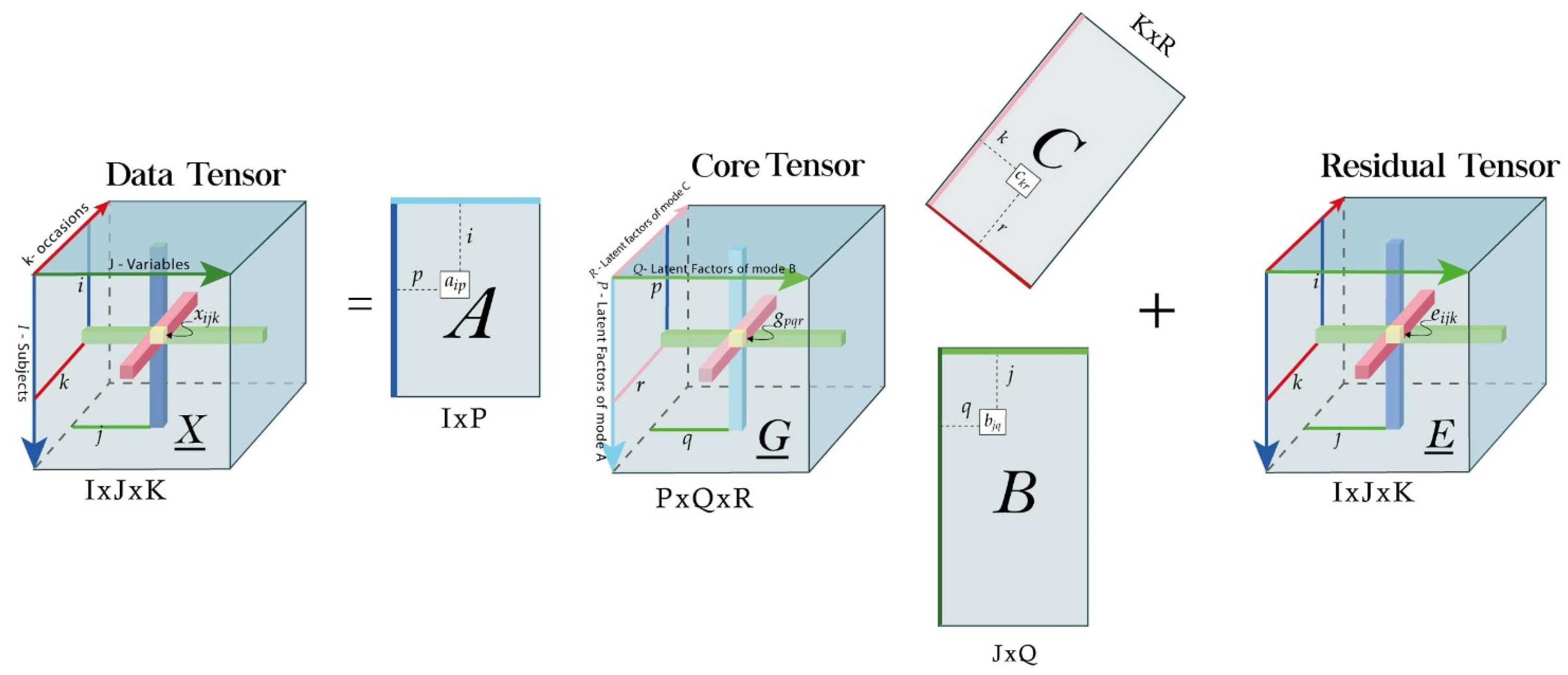
Figure 2.
Unfolding of the data tensor in its different modes.
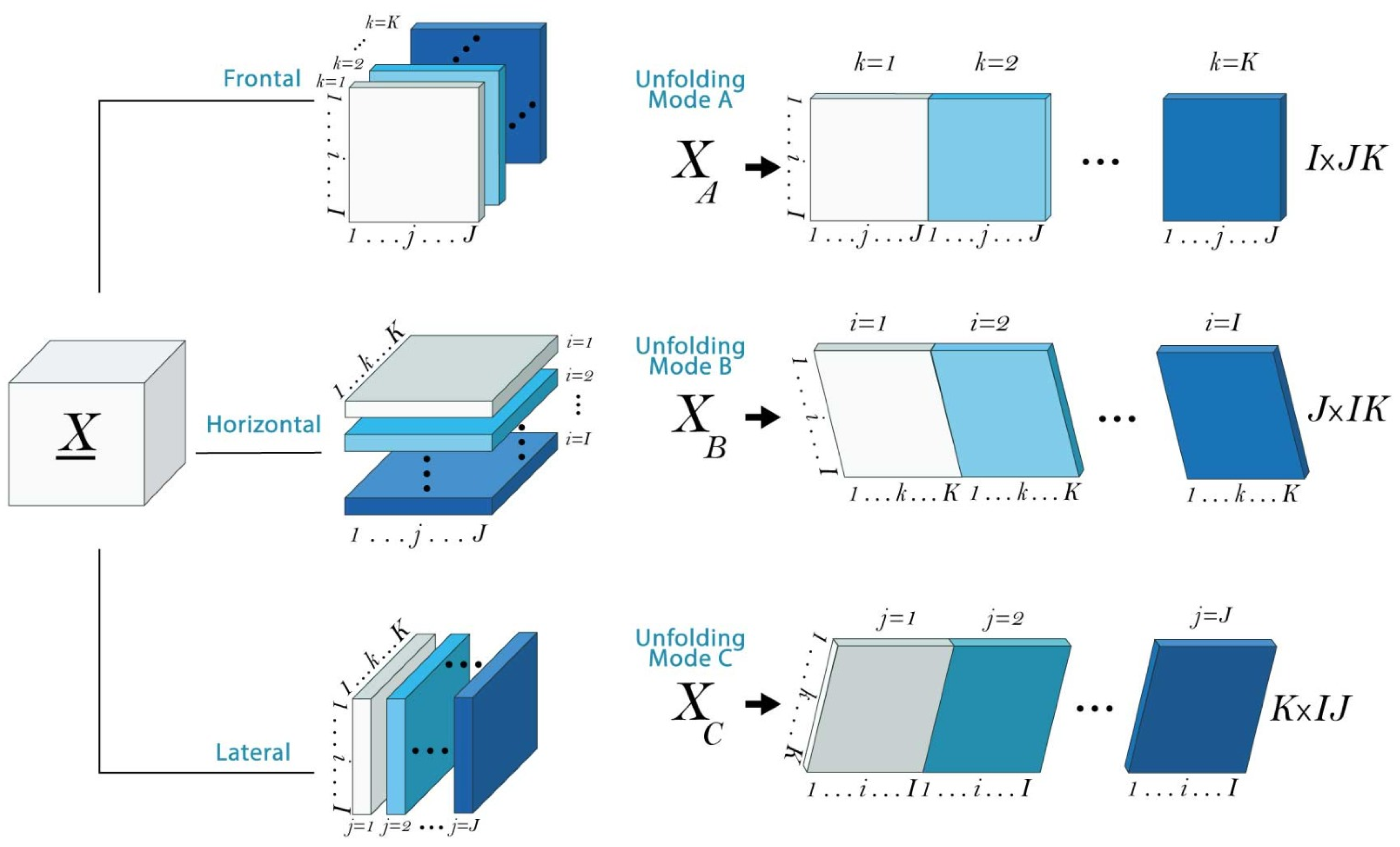
Figure 3.
Flowchart of the sample selection of articles related to Tucker Models from 2000 to 2023 according to the PRISMA 2020 statement.
Figure 3.
Flowchart of the sample selection of articles related to Tucker Models from 2000 to 2023 according to the PRISMA 2020 statement.
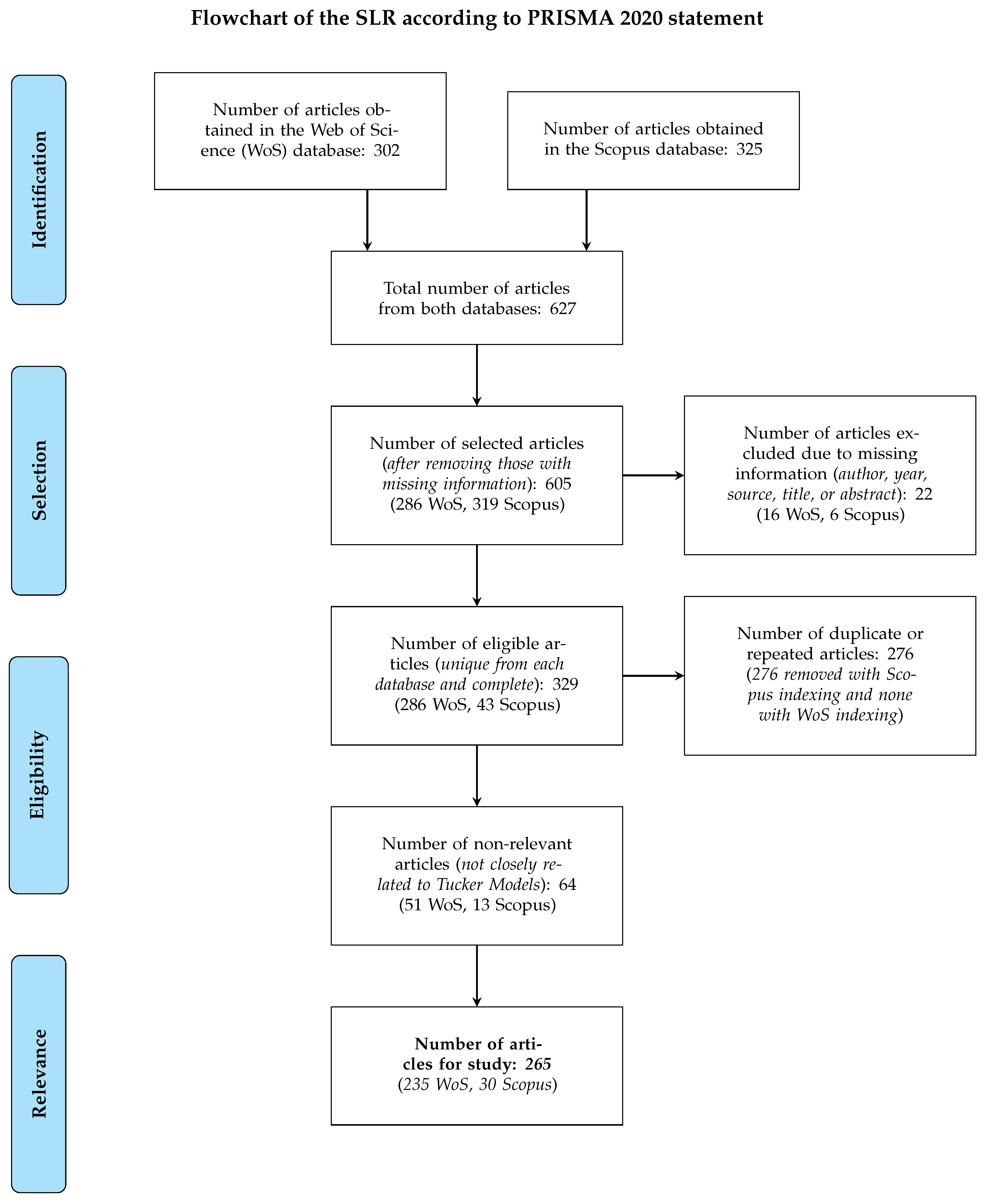
Figure 4.
Flowchart of the process for creating lexical tables with IraMuteq software.
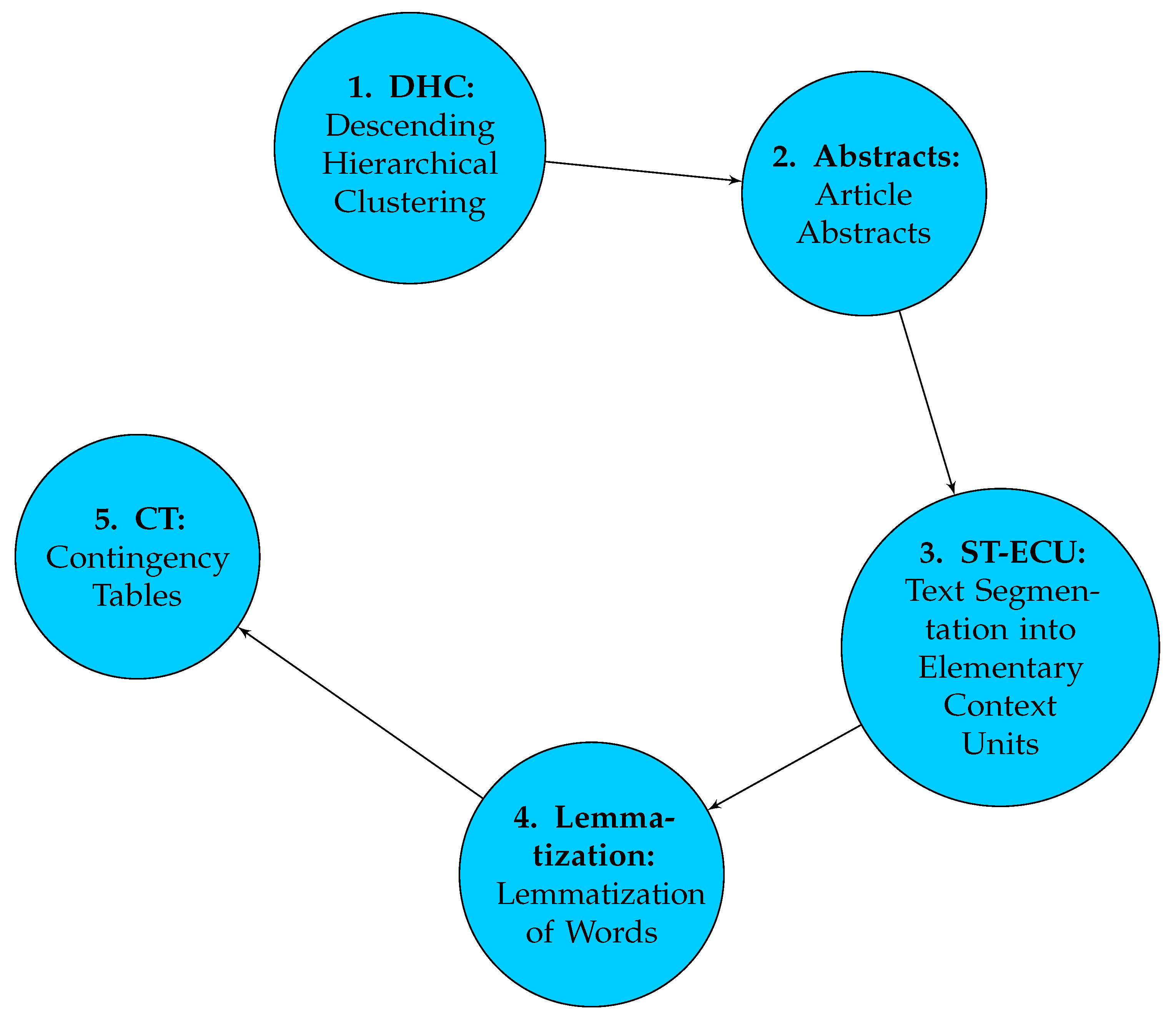
Figure 5.
Similarity graph of the textual corpus obtained by IraMuteq software.

Figure 6.
One-way MANOVA-Biplot obtained from the characterized lexical table.
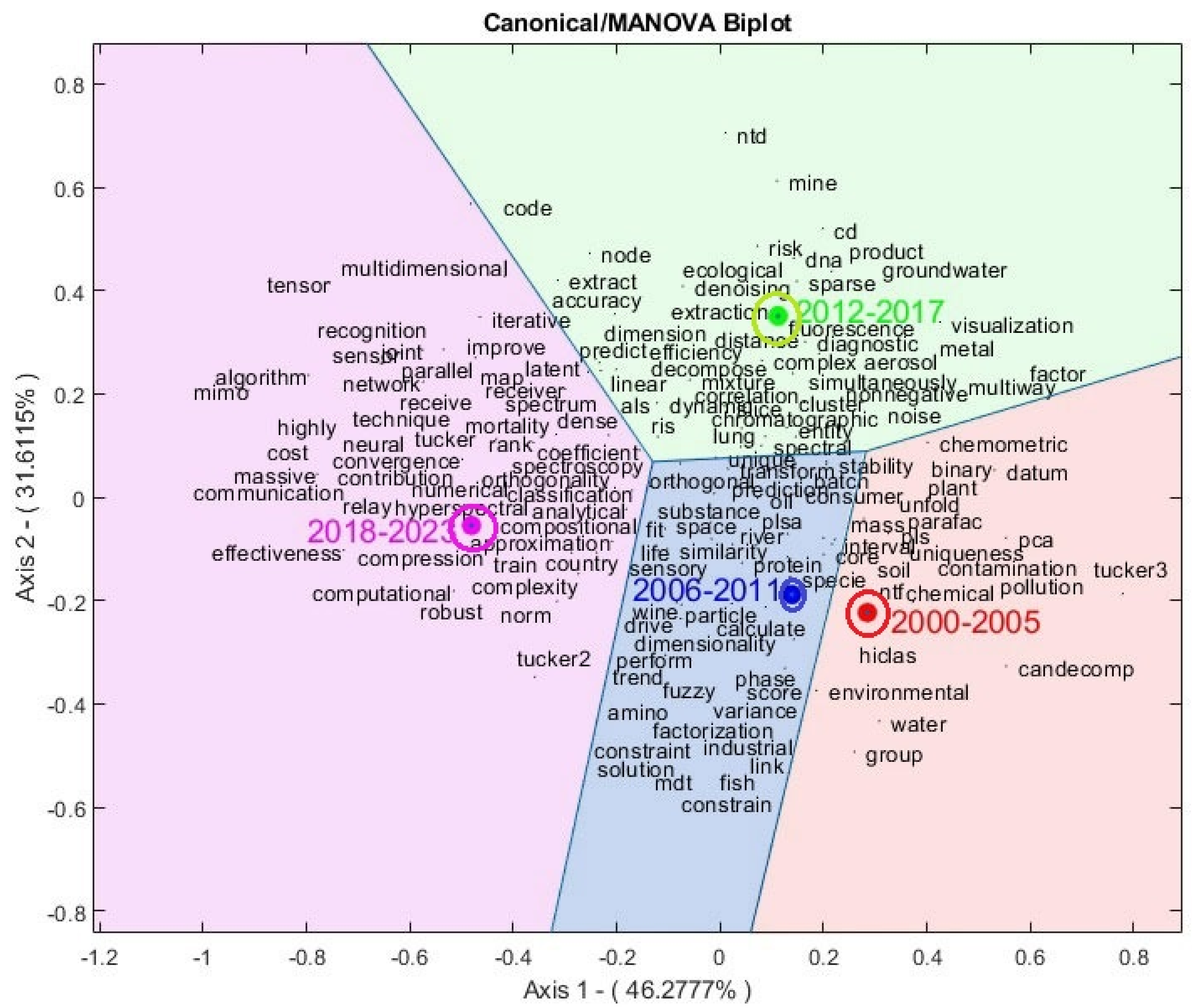
Figure 7.
Process of textual corpus analysis with ChatGPT 3.5.
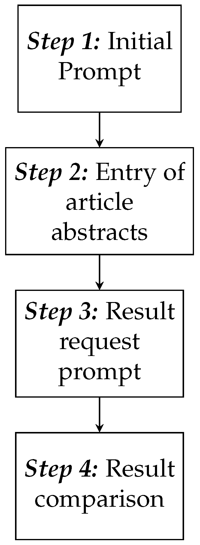
Figure 8.
Some prominent research on Tucker models from 2000 to 2023.
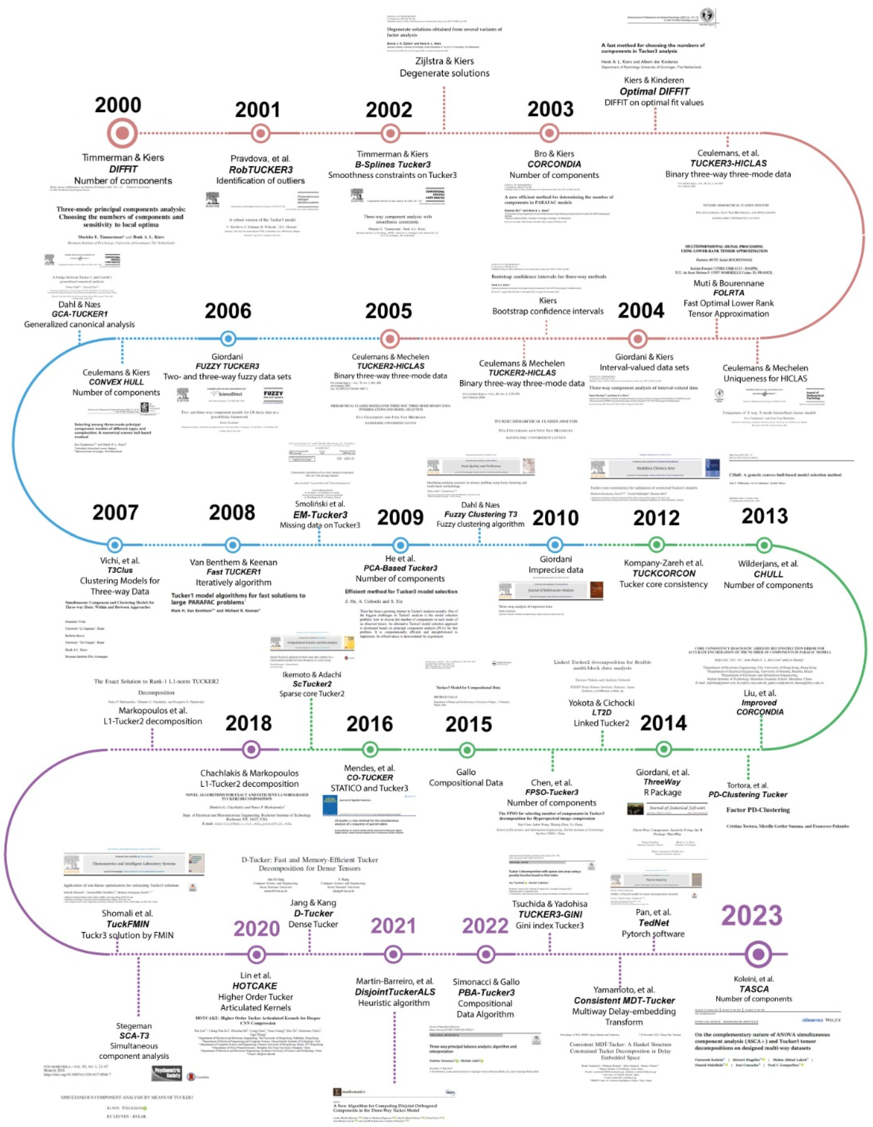

Table 1.
Partial result of Correspondence Factor Analysis from IraMuteq software
| *ID_1 | *ID_10 | ... | *ID_99 | |
|---|---|---|---|---|
| similarity | 0 | 0 | ... | 0 |
| dynamic | 0 | 0 | ... | 0 |
| calculate | 0 | 0 | ... | 0 |
| risk | 0 | 0 | ... | 0 |
| solution | 0 | 0 | ... | 0 |
| batch | 6 | 0 | ... | 0 |
| approximation | 0 | 0 | ... | 0 |
| tucker3 | 2 | 0 | ... | 0 |
| ... | ... | ... | ... | ... |
| validation | 0 | 0 | ... | 0 |
Table 2.
Simplified characterized frequency table
| ID | similarity | dynamic | calculate | ... | validation |
|---|---|---|---|---|---|
| *ID_1 | 0 | 0 | 0 | ... | 0 |
| *ID_10 | 0 | 0 | 0 | ... | 0 |
| *ID_100 | 0 | 0.169 | 0 | ... | 0 |
| *ID_101 | 0 | 0 | 0 | ... | 0 |
| *ID_102 | 0 | 0 | 0 | ... | 0 |
| *ID_103 | 0 | 0 | 0 | ... | 0 |
| ... | ... | ... | ... | ... | ... |
| *ID_99 | 0 | 0 | 0 | ... | 0 |
Table 3.
Correspondence between groups and article publication periods
| Group | Publication Period |
|---|---|
| 1 | January 1, 2000 - December 31, 2005 |
| 2 | January 1, 2006 - December 31, 2011 |
| 3 | January 1, 2012 - December 31, 2017 |
| 4 | January 1, 2018 - December 31, 2023 |
Table 4.
Eigenvalues and Variability between groups explained and cumulative.
| Dimension | Eigenv. | % Expl. | Cumm. | p-val |
|---|---|---|---|---|
| 1 | 20.49 | 46.28 | 46.28 | 0 |
| 2 | 16.94 | 31.61 | 77.89 | 0 |
| 3 | 14.17 | 22.11 | 100 | 0 |
Table 5.
Quality of representation of group means x1000.
| Group No. | Period | Axis 1 | Axis 2 | Cumulative |
|---|---|---|---|---|
| 1 | 2000-2005 | 340 | 209 | 549 |
| 2 | 2006-2011 | 153 | 282 | 435 |
| 3 | 2012-2017 | 93 | 907 | 1000 |
| 4 | 2018-2023 | 975 | 13 | 988 |
Table 6.
Strategies for Prompt Design in ChatGPT 3.5 and their impact.
| Strategy | Description | Impact on Results |
|---|---|---|
| Specificity and Context | Provide clear details about the task and objective of the query to reduce ambiguities. | Improves accuracy and relevance of the response. |
| Step-by-Step Structuring | Divide the query into sequential steps to better guide content generation. | Produces more organized and coherent responses. |
| Use of Examples and Constraints | Include specific examples and limit the scope of the response to avoid irrelevant information. | Reduces generic responses and improves information relevance. |
| Iterative Refinement | Reformulate prompts based on the initial output to improve accuracy and depth. | Adjusts the generated content to be more precise and aligned with the objectives. |
| Bias Control and Cross-Validation | Evaluate responses from different perspectives and verify information with external sources. | Minimizes errors, biases, and ensures more reliable information. |
Table 7.
Initial Prompt for article abstract analysis using ChatGPT 3.5.
| Prompt 1: | I will provide a set of research article abstracts. Your |
| task is to analyze them and extract key insights related to | |
| Tucker models. | |
| Prompt 2 | I will provide you with a table containing information from |
| 20 articles.The first column of this table is the year of | |
| publication, the second column contains the authors, and the | |
| third column contains the correspondingabstract of each | |
| article. In chronological order, identify and summarize the | |
| main findings and present the information grouped by year. |
Disclaimer/Publisher’s Note: The statements, opinions and data contained in all publications are solely those of the individual author(s) and contributor(s) and not of MDPI and/or the editor(s). MDPI and/or the editor(s) disclaim responsibility for any injury to people or property resulting from any ideas, methods, instructions or products referred to in the content. |
© 2025 by the authors. Licensee MDPI, Basel, Switzerland. This article is an open access article distributed under the terms and conditions of the Creative Commons Attribution (CC BY) license (http://creativecommons.org/licenses/by/4.0/).
Copyright: This open access article is published under a Creative Commons CC BY 4.0 license, which permit the free download, distribution, and reuse, provided that the author and preprint are cited in any reuse.


