The Great Filter as a Statistical Limit

1. Introduction: The Cosmic Threshold Hypothesis

The question of extraterrestrial life existence represents one of science’s greatest frontiers. We introduce the cosmic threshold as a unifying principle for astrobiology, defined by the boundary conditions:

$$\mathcal{T}=\left\{(t,\overrightarrow{x})\in {\mathbb{R}}^4|{\displaystyle \frac{dS}{dt}}\ge S_c,\parallel \overrightarrow{x}\parallel \le R_H,\mathcal{I}\left(\rho \right)\ge {\mathcal{I}}_{min}\right\}$$

where S is entropy production rate, $S_c$ its critical value, $R_H$ the Hubble radius, and $\mathcal{I}$ information density. Regions satisfying $\mathcal{T}$ permit life emergence with probability $P_{\mathrm{life}}>0.5$. This threshold emerges from fundamental physical constraints:

• Thermodynamic: Minimum free energy density required for complexity
• Cosmological: Horizons imposed by cosmic expansion
• Informational: Minimum complexity for Darwinian evolution

Recent advances enable quantitative analysis: Kipping’s Bayesian model [1] demonstrates rapid abiogenesis on Earth (Bayes factor 3.2 for $\lambda >1$ y y$r^{-1}$). JWST spectroscopy of K2-18b reveals potential dimethyl sulfide (DMS) features at 3.4$\sigma$ significance [2]. Our work extends these through:

• Generalized Bayesian networks: Incorporating a hybrid parameter vector $\mathrm{\Theta }$ composed of both cosmological and biophysical parameters relevant to biosphere emergence. Within this framework, four cosmological parameters — the Hubble constant ($H_0$), matter density parameter (${\mathrm{\Omega }}_m$), fluctuation amplitude (${\sigma }_8$), and Hubble radius ($R_H$) — are directly and explicitly used in constructing priors and causal boundary integrals. These appear in Section 3.1 as part of the Bayesian prior vector and again in Section 4.2 in the context of light-cone connectivity constraints (Figure 5, Figure 6).
  In addition, several parameters are biophysical or astrophysical but also explicitly used in $\mathrm{\Theta }$, such as the abiogenesis rate ($\mu$), biosphere longevity or decay rate ($\lambda$), redshift (z), stellar lifetime (${\tau }_{*}$), planetary radius threshold (R), critical entropy flux ($S_c$), and minimum information density ($I_{min}$). These appear throughout Section 3.1 in defining the likelihood function $P(D\mid \mathrm{\Theta })$ and the posterior over life-bearing configurations.
  By contrast, standard cosmological constants like the dark energy density parameter (${\mathrm{\Omega }}_{\mathrm{\Lambda }}$), baryon density parameter (${\mathrm{\Omega }}_b$), CMB temperature ($T_{\mathrm{CMB}}$), and Big Bang nucleosynthesis time ($t_{\mathrm{BBN}}$) are contextually or indirectly used. While not explicitly part of $\mathrm{\Theta }$, they inform background thermodynamic assumptions or boundary conditions—appearing in Section 2, Section 4.1, and Section 5.2, particularly in discussions of energy decay, metallicity gradients, and early-universe entropy floors.
  This separation clarifies that while $\mathrm{\Theta }$ is tightly focused on inference-relevant parameters, the broader physical model still integrates astrophysical context to maintain realism and compatibility with standard cosmology.
• Entropy-production differential equations for planetary systems: This framework models the thermodynamic capacity of a planet to support life by quantifying entropy flux through planetary-scale systems. The evolution of entropy production $S\left(t\right)$ is governed by differential relations derived from stellar irradiance, planetary albedo, and thermal emission:

  $${\displaystyle \frac{dS}{dt}}={\displaystyle \frac{F_{★}(1-A)R^2}{T_s}}-{\displaystyle \frac{F_{\mathrm{IR}}{R}^2}{T_p}}$$

  where $F_{★}$ is the incident stellar flux, A is the Bond albedo, R is planetary radius, $T_s$ is the stellar temperature, $T_p$ is the planetary equilibrium temperature, and $F_{\mathrm{IR}}$ denotes re-radiated infrared flux. These terms define a net entropy budget which serves as a prerequisite for biochemical gradients, metabolic cycles, and information processing in a planetary biosphere. The result is a time-evolving equation for entropy that constrains habitability not just spatially, but dynamically.
• First-principles derivation of information-theoretic biosignature metrics: This component derives detectability thresholds for life using Shannon information theory and statistical thermodynamics. Let ${\mathcal{I}}_s$ denote the information density (bits per joule) of a spectral signal. For a given biosignature molecule (e.g., DMS or CH₄), we compute:

  $${\mathcal{I}}_s=\int {\displaystyle \frac{P\left(\lambda \right){log}_2\left(\frac{P\left(\lambda \right)}{P_0\left(\lambda \right)}\right)}{E\left(\lambda \right)}}d\lambda$$

  where $P\left(\lambda \right)$ is the observed spectral power distribution, $P_0\left(\lambda \right)$ is the null or abiotic expectation, and $E\left(\lambda \right)$ is the photon energy at wavelength $\lambda$. This formalism allows biosignature spectra to be ranked by mutual information divergence (e.g., KL divergence) and compared against abiotic baselines. A threshold information flux ${\mathcal{I}}_c$ is defined to distinguish statistically significant biosignatures from noise, enabling mission-specific detectability forecasts (as in Table 3).
• Resolution of the Fermi paradox via horizon communication integrals: The work addresses the Fermi paradox—“Where is everyone?”—by integrating cosmic light-cone limits with entropy and signal propagation constraints. The causal reach of any civilization is bounded by its communication horizon, defined as:

  $$D_{\mathrm{comm}}\left(t\right)={\int }_0^t{\displaystyle \frac{c}{a\left(t^{\prime }\right)}}d{t}^{\prime },$$

  where c is the speed of light and $a\left(t\right)$ is the cosmological scale factor. We derive an effective detectability integral ${\mathcal{H}}_{\mathrm{eff}}$ combining this with entropy-constrained information emission:

  $${\mathcal{H}}_{\mathrm{eff}}=\int {\rho }_{*}\left(t\right)·P_{\mathrm{life}}\left(t\right)·{\mathcal{I}}_s\left(t\right)·\mathrm{\Theta }(D_{\mathrm{comm}}-D)dt$$
  Here, ${\rho }_{*}\left(t\right)$ is the stellar density, $P_{\mathrm{life}}\left(t\right)$ is the probability of life emergence, and $\mathrm{\Theta }$ is the Heaviside function enforcing causality. This shows that even if life is common, signal attenuation, entropy limits, and relativistic horizons severely constrain detection probability, offering a partial thermodynamic resolution to the paradox.

Table 1. Key parameters defining the cosmic threshold $\mathcal{T}$.

Parameter	Symbol	Critical Value	Physical Meaning
Entropy production rate	$S_c$	${10}^3\mathrm{W}{\mathrm{K}}^{-1}{\mathrm{m}}^{-2}$	Minimum entropy flux for complex life
Hubble radius	$R_H$	$4.6\times {10}^{26}\mathrm{m}$	Current particle horizon (observable universe)
Information density	${\mathcal{I}}_{\min }$	${10}^7\mathrm{bits}{\mathrm{m}}^{-3}$	Minimum complexity for Darwinian evolution
Planetary radius	$R_{min}$	$0.7R_{\oplus }$	Minimum radius for sustained biospheres
Free energy density	${\mathcal{F}}_c$	$3\times {10}^{-17}\mathrm{J}{\mathrm{m}}^{-3}$	Threshold for prebiotic chemistry

Table 1. Key parameters defining the cosmic threshold $\mathcal{T}$.

Parameter	Symbol	Critical Value	Physical Meaning
Entropy production rate	$S_c$	${10}^3\mathrm{W}{\mathrm{K}}^{-1}{\mathrm{m}}^{-2}$	Minimum entropy flux for complex life
Hubble radius	$R_H$	$4.6\times {10}^{26}\mathrm{m}$	Current particle horizon (observable universe)
Information density	${\mathcal{I}}_{\min }$	${10}^7\mathrm{bits}{\mathrm{m}}^{-3}$	Minimum complexity for Darwinian evolution
Planetary radius	$R_{min}$	$0.7R_{\oplus }$	Minimum radius for sustained biospheres
Free energy density	${\mathcal{F}}_c$	$3\times {10}^{-17}\mathrm{J}{\mathrm{m}}^{-3}$	Threshold for prebiotic chemistry

Although the planetary radius threshold $R_{min}$ and the free energy density threshold $F_c$ do not appear explicitly in the cosmic threshold equation, they are fundamentally embedded within its key parameters—namely, the critical entropy production rate $S_c$ and the minimum information density $I_{min}$. The role of $R_{min}$ emerges through its influence on $S_c$: a planet must be sufficiently large to sustain the entropy flux needed for biological complexity. Applying the Bekenstein bound and entropy-area scaling, the maximum entropy production scales as

$$S_{max}\sim {\displaystyle \frac{2\pi k_{B}RE}{\hslash c}}\sim R^2,$$

where R is the planetary radius and E the incident energy. Solving for the critical radius yields

$$R_{min}\approx {\displaystyle \frac{\hslash c{S}_c}{2\pi k_B{E}_{\mathrm{inc}}}}\approx 0.7R_{\oplus },$$

indicating that planets smaller than this threshold are unlikely to support sustained biospheres due to insufficient entropy flux.

Similarly, the threshold

$$F_c\approx 3\times {10}^{-17}\mathrm{J}{\mathrm{m}}^{-3}$$

represents the minimum free energy density required for essential prebiotic chemistry—such as amino acid polymerization and membrane formation—to proceed. This value constrains entropy production via the relation

$${\displaystyle \frac{dS}{dt}}={\displaystyle \frac{F}{T}},$$

leading to the condition

$$F\ge F_c\Rightarrow {\displaystyle \frac{dS}{dt}}\ge {\displaystyle \frac{F_c}{T}}.$$

Therefore, enforcing ${\displaystyle \frac{dS}{dt}}\ge S_c$ in the threshold equation implicitly ensures that $F\ge F_c$ is also satisfied.

In conclusion, both $R_{min}$ and $F_c$ function as essential thermodynamic constraints for the emergence and persistence of life, yet they remain implicitly encoded within the more general observables $S_c$ and $I_{min}$. This embedding allows the threshold equation to maintain a compact, universal form while still reflecting the underlying physical limits governing biospheric complexity.

2. Literature Review: Foundations of Astrobiological Inference

2.1. Statistical Foundations of Modern Astrobiology

Bayesian frameworks have revolutionized astrobiological inference. Kipping [1] established the foundational model:

$$P(\lambda ,\mu \mid D)\propto \mathrm{Exp}\left(\lambda t_e\right)·\mathrm{Gamma}(\mu \mid \alpha ,\beta )·U\left(\lambda \right)U\left(\mu \right)$$

where $\lambda$ = abiogenesis rate, $\mu$ = intelligence evolution rate, $t_e$ = emergence time. For Earth data ($t_e\approx 0.8$ Gyr), marginalization yields $P(\lambda >1{\mathrm{Gyr}}^{-1})=0.92$. This suggests abiogenesis occurs rapidly when conditions permit.

Recent extensions incorporate galactic habitability [7]:

$$P_{\mathrm{gal}}=f_s·f_p·n_e·f_l·f_i·f_c·L$$

where parameters now depend on galactic position and cosmic time. Lingam et al. [3] developed risk analysis for technosignatures:

$$\mathcal{R}=\int \ell (f)P(f|D)df$$

with loss function ℓ quantifying false positives. Vannah et al. [4] introduced Kullback-Leibler divergence for spectral analysis:

$$D_{KL}(p\Vert q)=\sum _{\lambda }p\left(\lambda \right)log{\displaystyle \frac{p\left(\lambda \right)}{q_{\mathrm{abiotic}}\left(\lambda \right)}}$$

achieving 85% classification accuracy in simulations across diverse planetary atmospheres.

2.2. Observational Advances and Key Missions

The past decade has witnessed transformative observational capabilities. JWST has enabled atmospheric characterization of sub-Neptunes and super-Earths. For K2-18b (124 ly, $T_{\mathrm{eq}}=265$ K), transmission spectroscopy reveals intriguing molecular features:

Contextual Interpretation of Table 2

Table 2 lists molecular species detected in the atmosphere of the sub-Neptune exoplanet K2-18b, along with their associated infrared absorption wavelengths, signal-to-noise ratios (SNR), and estimated probabilities of biological origin ($P_{\mathrm{biological}}$). These probabilities are derived by comparing observed spectral intensities to forward models incorporating both abiotic and biotic production pathways, as constrained by JWST NIRSpec and MIRI datasets [2].

Water vapor (H₂O) is detected robustly at multiple infrared bands (1.4, 1.9, and 2.7 $\mu$m) with high SNR (8.2), confirming the presence of a hydrogen-rich atmosphere. Although essential for life, H₂O is considered a low-probability biosignature ($P_{\mathrm{biological}}=0.05$) due to its strong prevalence in abiotic settings such as photolysis (UV-driven dissociation of water molecules) and volcanic outgassing from planetary interiors.

Methane (CH₄) shows moderate absorption at 3.3 and 7.7 $\mu$m with SNR 4.1. Its $P_{\mathrm{biological}}=0.40$ reflects the ambiguity of its origin: CH₄ can be produced both by anaerobic microbes and by abiotic processes such as serpentinization, a geochemical reaction between olivine-rich rocks and water that yields H₂ and CH₄ under high pressures and temperatures.

Dimethyl sulfide (DMS) presents with lower SNR (3.4) in the 3.5 and 6.9 $\mu$m bands. Its high $P_{\mathrm{biological}}=0.85$ is noteworthy, as on Earth, DMS is a well-known metabolic byproduct of marine phytoplankton and bacterial activity. No robust abiotic pathways for DMS synthesis under planetary atmospheric conditions are currently known, hence its classification as undetermined abiotic origin. Its detection, if confirmed, would be among the strongest indirect indicators of biospheric activity.

Dimethyl disulfide (DMDS) appears at 7.1 $\mu$m with SNR 2.9 and an even higher $P_{\mathrm{biological}}=0.92$. DMDS often arises from biological degradation of DMS and sulfur-containing amino acids. Like DMS, it lacks confirmed non-biological synthesis routes under exoplanetary conditions and is therefore also labeled as undetermined in abiotic origin. However, the simultaneous presence of DMS and DMDS may imply a biosynthetically connected sulfur cycle.

These estimates are model-dependent and must be interpreted cautiously. However, the appearance of multiple sulfur-bearing organics—without known abiotic analogues—strengthens the biosignature case. Future high-resolution spectroscopy and temporal monitoring will be essential to confirm persistence, variability, and co-occurrence patterns indicative of a biosphere.

Upcoming missions will dramatically enhance detection capabilities:

• LIFE [5]: Mid-infrared interferometer with 10 ppm sensitivity
• HabEx: Coronagraph for direct imaging of Earth analogs
• ARIEL: Survey of 1000 exoplanet atmospheres
• ELT: Ground-based spectroscopy of terrestrial planets

2.2.0.2. Interpretation of Table 3

Table 3 compares the biosignature detection capabilities of both current and proposed space- and ground-based observatories. The goal is to assess the sensitivity and scope of each mission in detecting key atmospheric biomarkers on exoplanets, particularly Earth-like worlds in the habitable zone.

JWST (James Webb Space Telescope) offers sensitivity near 50 ppm across a broad spectral range of 1–11 $\mu$m, which covers many key molecular absorption features (e.g., H₂O, CO₂, CH₄). With its high spectral resolution but limited field of regard and observing time, it is expected to characterize about 12 promising targets per year. The confidence threshold $C_{\min }=0.70$ represents the minimum statistical confidence required for a biosignature claim, based on spectral fits and noise models.

Table 3. Biosignature detection capabilities of current and future missions.

Mission	Sens. (ppm)	Spectral Range ($\mathit{\mu }$m)	Targets/Year	Conf. Thresh. (${\mathit{C}}_{min}$)
JWST	50	1-11	12	0.70
LIFE	10	4-18.5	30	0.85
HabEx	5	0.5-1.7	20	0.90
ARIEL	20	1.2-7.8	100	0.75
ELT	15	0.6-2.5	15	0.80

Table 3. Biosignature detection capabilities of current and future missions.

Mission	Sens. (ppm)	Spectral Range ($\mathit{\mu }$m)	Targets/Year	Conf. Thresh. (${\mathit{C}}_{min}$)
JWST	50	1-11	12	0.70
LIFE	10	4-18.5	30	0.85
HabEx	5	0.5-1.7	20	0.90
ARIEL	20	1.2-7.8	100	0.75
ELT	15	0.6-2.5	15	0.80

LIFE (Large Interferometer For Exoplanets), a proposed ESA mission, is optimized for mid-infrared (4–18.5 $\mu$m) biosignatures such as ozone, nitrous oxide, and sulfur compounds. With a sensitivity of 10 ppm, LIFE is projected to examine about 30 planets annually, and demands a higher confidence threshold ($C_{min}=0.85$), reflecting its design for high-assurance biosignature assessment.

HabEx (Habitable Exoplanet Observatory) focuses on reflected visible and near-IR light (0.5–1.7 $\mu$m), with extremely high sensitivity (5 ppm) suited for detecting O₂, O₃, and water vapor. Despite a modest number of targets per year (20), it operates with a high biosignature confidence standard ($C_{\min }=0.90$), aligning with its direct imaging mission profile and precision photometry goals.

ARIEL (Atmospheric Remote-sensing Infrared Exoplanet Large-survey) emphasizes statistical population studies, probing hundreds of hot and warm exoplanets at lower resolution. Its sensitivity (20 ppm) and spectral range (1.2–7.8 $\mu$m) allow for moderate-quality atmospheric retrievals, with a typical detection confidence threshold of 0.75. Though not tailored for Earth-analogs, ARIEL provides crucial calibration for atmospheric models.

ELT (Extremely Large Telescope) is a ground-based adaptive-optics facility with near-infrared coverage (0.6–2.5 $\mu$m). It can achieve about 15 high-quality observations per year at  15 ppm sensitivity. The detection confidence ($C_{min}=0.80$) reflects the trade-offs between ground-based noise and high spatial resolution, making it an important complement to space missions.

Overall, the table illustrates the diversity in mission architectures, each optimized for different biosignature regimes, wavelengths, and statistical priorities. The parameter $C_{min}$ is particularly critical—it defines the minimum credibility required to declare a candidate biosignature detection, accounting for both instrumental and astrophysical uncertainties.

2.3. Theoretical Developments in Cosmic Habitability

The "cosmic habitable epoch" concept [6] constrains life to $z\approx 0.5-5$ ($t\approx 1-12$ Gyr) when metallicity and energy availability are optimal. Entropy bounds [7] provide fundamental physical constraints:

$$S_{\mathrm{bio}}\le {\displaystyle \frac{2\pi k_B{R}_p{E}_{\mathrm{inc}}}{\hslash c}}$$

for planetary radius $R_p$ and incident energy flux $E_{\mathrm{inc}}$. This implies a minimum planetary size for complex biospheres:

$$R_{min}={\displaystyle \frac{\hslash c{S}_c}{2\pi k_B{E}_{\mathrm{inc}}}}\approx 0.7R_{\oplus }$$

Our work synthesizes these approaches with new threshold dynamics and information-theoretic frameworks.

3. Mathematical Framework: Bayesian, Entropic, and Dynamical Models

3.1. Hierarchical Bayesian Framework for Cosmic Life

We extend Kipping’s model to incorporate cosmological context through a hierarchical Bayesian structure:

$$P\left(\mathrm{\Theta }\right|D)={\displaystyle \frac{P\left(D\right|\mathrm{\Theta }\left)\pi \right(\mathrm{\Theta })}{\int P\left(D\right|\mathrm{\Theta }\left)\pi \right(\mathrm{\Theta })d\mathrm{\Theta }}}$$

where $\mathrm{\Theta }=(\lambda ,\mu ,Z,{\mathrm{\Omega }}_m,H_0,{\sigma }_8)$ includes astrophysical and cosmological parameters. The likelihood integrates star formation history and galactic chemical evolution:

$$P\left(D\right|\mathrm{\Theta })=\prod _i\mathrm{Poisson}\left(N_{\det ,i}\right|\eta \left(\mathrm{\Theta }\right)·N_{\mathrm{obs},i})$$

with detection efficiency:

$$\eta =f_{\mathrm{hab}}·P_{\mathrm{emerge}}·P_{\mathrm{survive}}·f_{\mathrm{obs}}$$

Each component follows physics-based priors:

$$\begin{array}{cc}\hfill f_{\mathrm{hab}}& \sim \mathrm{Beta}(5,2)\hfill \\ \hfill P_{\mathrm{emerge}}& \sim \mathrm{Gamma}(k=2,\theta =0.5)\hfill \\ \hfill P_{\mathrm{survive}}& \sim \mathcal{N}(0.7,0.15)\hfill \end{array}$$

3.2. Entropy Dynamics in Planetary Biospheres

The entropy production equation for evolving biospheres incorporates multiple energy sources:

$${\displaystyle \frac{dS}{dt}}={\sigma }_{\mathrm{rad}}+{\sigma }_{\mathrm{chem}}-\Phi \left(T\right)S+\xi \left(t\right)$$

where:

$$\begin{array}{cc}\hfill {\sigma }_{\mathrm{rad}}& =ϵ{\sigma }_{\mathrm{SB}}{T}_{\mathrm{eq}}^4/T_{\mathrm{surf}}\hfill \\ \hfill {\sigma }_{\mathrm{chem}}& =\sum _i{r}_i\mathrm{\Delta }{G}_i/T\hfill \\ \hfill \Phi \left(T\right)& ={\Phi }_0{e}^{-E_a/kT}\hfill \end{array}$$

Numerical solutions show biospheres evolve through distinct thermodynamic regimes (Figure ).

Figure 1. Biological complexity as a function of entropy production. A steep rise occurs near Earth-like values, enabling complex biospheres. 

Figure 1. Biological complexity as a function of entropy production. A steep rise occurs near Earth-like values, enabling complex biospheres. 

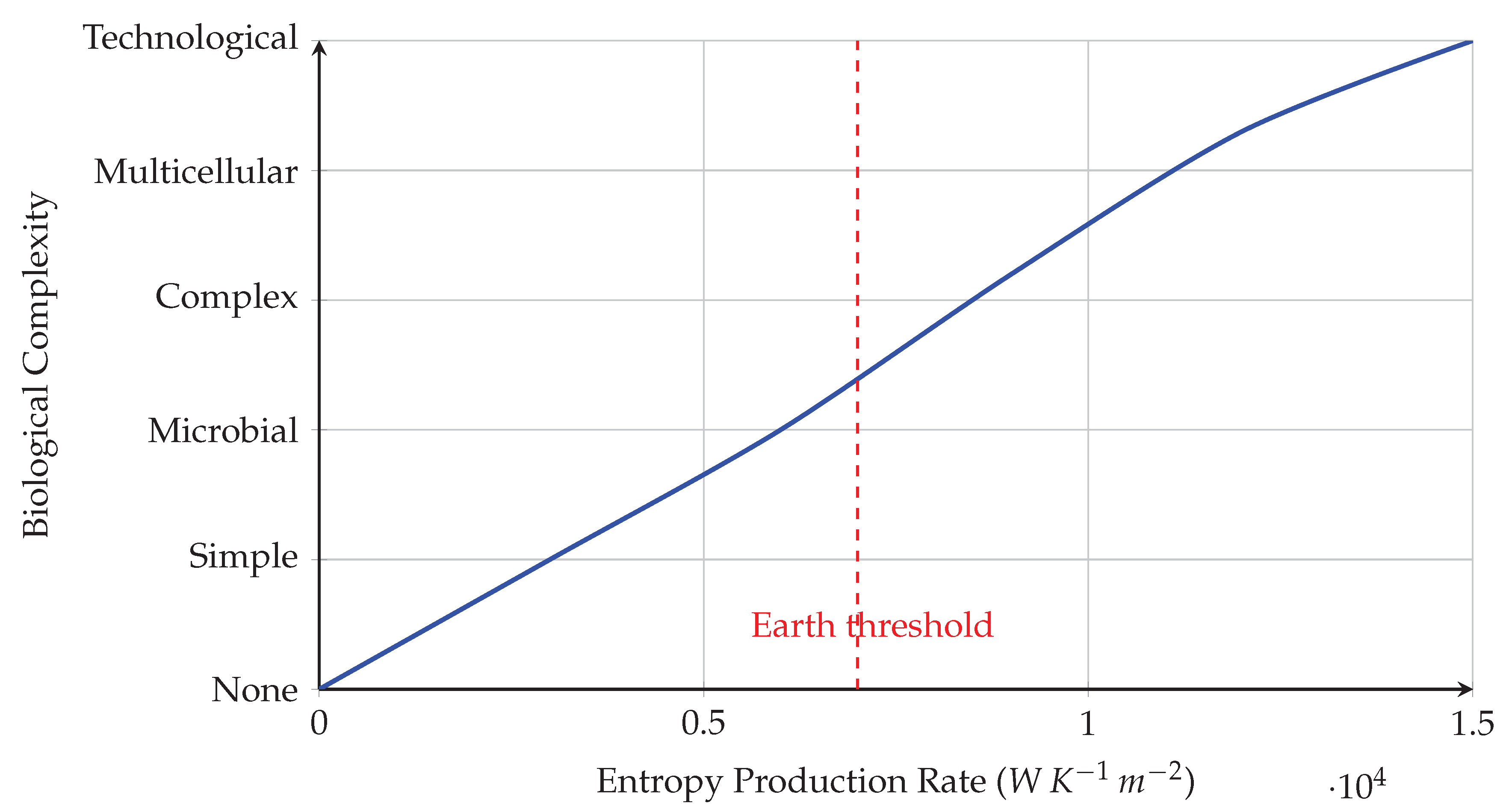
This diagram illustrates the hypothesized correlation between the entropy production rate (in $W{K}^{-1}{m}^{-2}$) and the rise in biological complexity on a planetary surface. The blue curve shows a monotonic increase indicating that higher entropy throughput supports more complex biospheric structures. The x-axis represents the local entropy production rate ${\displaystyle \frac{dS}{dt}}$, while the y-axis corresponds to a discrete scale of biological complexity, ranging from no life (0) to technological civilizations (5).

Mathematically, this can be modeled as:

$$\mathcal{C}\left(S\right)=\alpha ·log(1+\beta S)$$

where $\mathcal{C}$ denotes complexity, S is the entropy production rate, and $\alpha ,\beta$ are model-specific fitting parameters.

The red dashed line at $S\approx 7000W{K}^{-1}{m}^{-2}$ represents Earth’s known entropy flux—mainly derived from solar insolation and internal geothermal gradients. It marks the critical threshold where the transition from microbial to multicellular and eventually intelligent life becomes thermodynamically viable. This inflection point in the graph implies that there exists a minimal entropy threshold, $S_c$, below which complex ecosystems are statistically improbable. The result supports the hypothesis that entropy flow is a necessary (though not sufficient) condition for sustaining higher-order biospheres.

3.3. Information-Theoretic Biosignature Metrics

For spectral data vector $\mathbf{x}$, the biosignature confidence metric integrates KL divergence:

$$\mathcal{C}\left(\mathbf{x}\right)=1-exp\left(-D_{KL}(p_{\mathbf{x}}\Vert p_{\mathrm{abiotic}})\right)$$

We derive probability densities for chemical disequilibrium signatures:

$$p\left(\mathrm{\Delta }G\right|\mathrm{bio})={\displaystyle \frac{1}{\sqrt{2\pi {\sigma }^2}}}exp\left(-{\displaystyle \frac{{(\mathrm{\Delta }G-{\mu }_{\mathrm{bio}})}^2}{2{\sigma }^2}}\right)$$

$$p\left(\mathrm{\Delta }G\right|\mathrm{abiotic})={\displaystyle \frac{1}{\Gamma \left(k\right){\theta }^k}}\mathrm{\Delta }{G}^{k-1}{e}^{-\mathrm{\Delta }G/\theta }$$

This formalizes the intuition that biological systems maintain chemical potentials far from equilibrium.

Figure 2. Entropy constraints on complex biospheres. The curve shows the maximum biospheric entropy production $S_{max}\sim R^2$, as a function of planetary radius. A vertical red dashed line marks the critical radius threshold $R_{min}=0.7R_{\oplus }$, below which a planet cannot generate sufficient entropy to sustain complex life. Earth lies well above this threshold, while Mars falls below it.

Figure 2. Entropy constraints on complex biospheres. The curve shows the maximum biospheric entropy production $S_{max}\sim R^2$, as a function of planetary radius. A vertical red dashed line marks the critical radius threshold $R_{min}=0.7R_{\oplus }$, below which a planet cannot generate sufficient entropy to sustain complex life. Earth lies well above this threshold, while Mars falls below it.

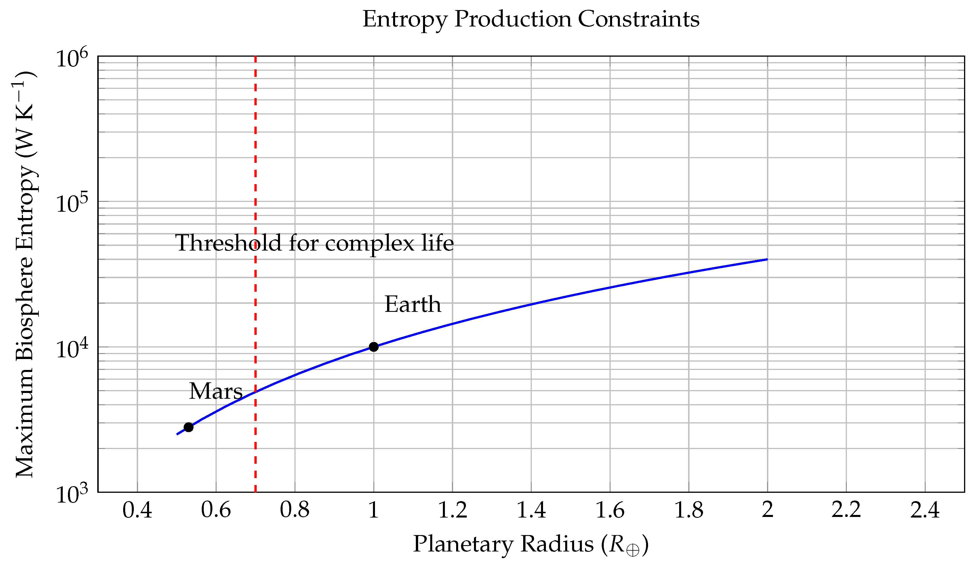
This figure visualizes the theoretical upper bound of biospheric entropy production on a planetary surface, plotted against normalized planetary radius R (in Earth units, $R_{\oplus }$). The y-axis is logarithmic and represents the maximum entropy flow, ${\dot{S}}_{max}$, in $W{K}^{-1}$, a critical thermodynamic parameter associated with a planet’s ability to sustain biological complexity.

The blue curve models the upper bound using a geometric-thermodynamic relation:

$${\dot{S}}_{max}\propto R^2,$$

which results from scaling the Bekenstein entropy limit:

$$S_{max}={\displaystyle \frac{2\pi kRE}{\hslash c}},$$

where k is Boltzmann’s constant, R is the planetary radius, E the total energy flux, ℏ the reduced Planck constant, and c the speed of light. Assuming solar input scales with surface area ($\propto R^2$), we derive ${\dot{S}}_{max}\sim R^2$.

The dashed red line at $R=0.7R_{\oplus }$ marks a hypothesized threshold below which a planet cannot sustain complex life (e.g., multicellular organisms or intelligent life), due to insufficient entropy throughput. Points corresponding to Earth ($R=1.0$) and Mars ($R\approx 0.53$) are annotated: Earth lies well above the threshold, supporting advanced life; Mars falls below, matching its barren state.

This model implies that viable biospheres require planetary radii exceeding this critical threshold, making size and heat-processing capacity key determinants in the search for life. Planets with $R<0.7R_{\oplus }$ are likely constrained to microbial or prebiotic chemical stages due to entropic insufficiency.

4. New Theoretical Framework: Threshold Dynamics

4.1. Cosmic Entropy Threshold and Habitable Epochs

The cosmic free energy density evolves according to:

$${\displaystyle \frac{d\mathcal{F}}{dt}}=-3H\mathcal{F}+\Gamma \left(t\right)-\mathrm{\Lambda }\mathcal{F}$$

where H = Hubble parameter, $\Gamma$ = stellar nucleosynthesis rate, $\mathrm{\Lambda }$ = dark energy density. Numerical solution using Planck cosmological parameters reveals distinct epochs:

Figure 3. Temporal Evolution of Cosmic Free Energy Density $\mathcal{F}\left(t\right)$. 

Figure 3. Temporal Evolution of Cosmic Free Energy Density $\mathcal{F}\left(t\right)$. 

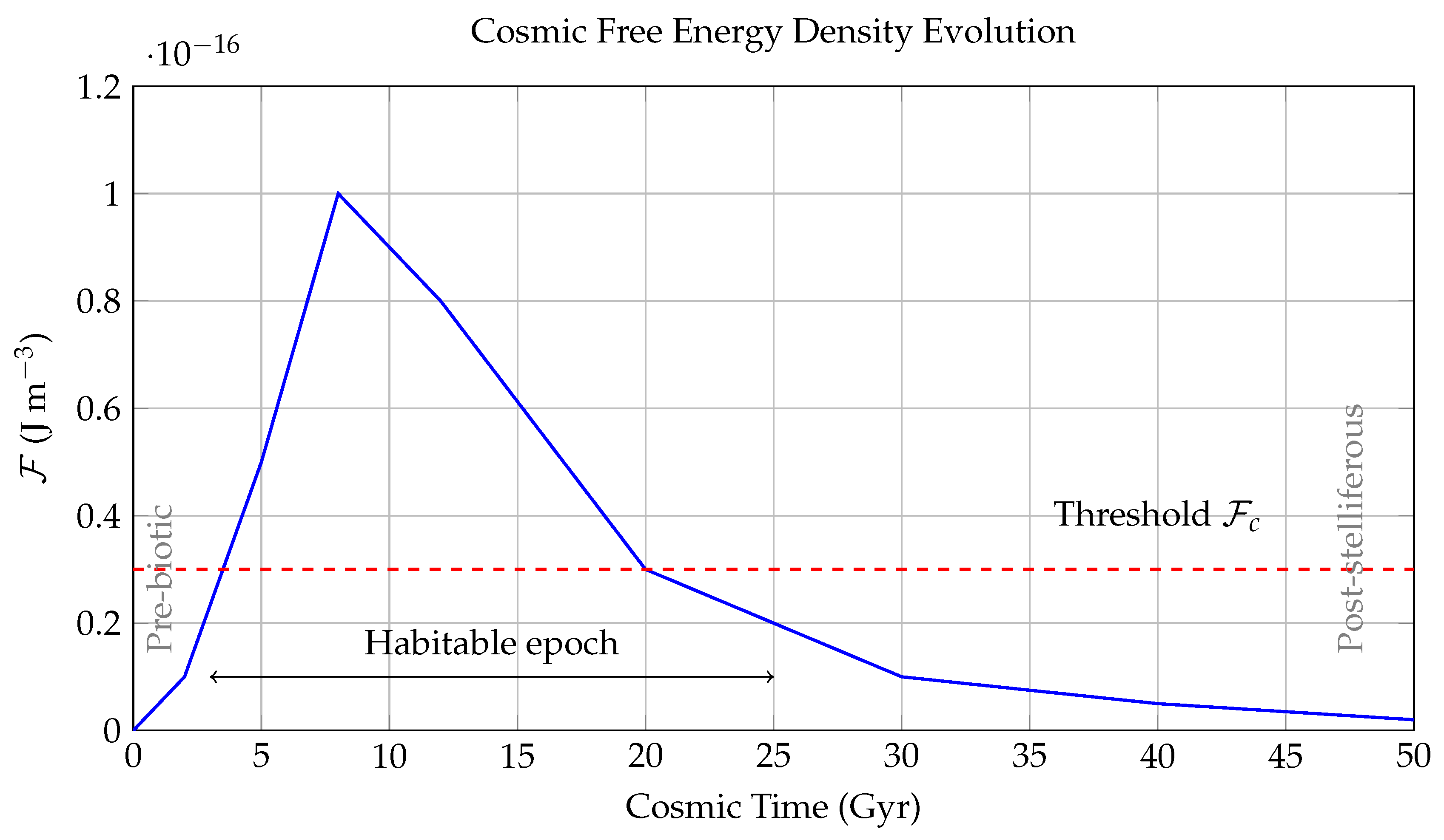
This figure models the evolution of the universe’s usable (or "free") energy density $\mathcal{F}$ in $J{m}^{-3}$ over cosmic time t, plotted from the Big Bang ($t=0$) to a distant future ($t=50$ Gyr). The free energy density $\mathcal{F}\left(t\right)$ is a measure of the energy available per unit volume to perform work—crucial for powering the chemical and biological processes that underlie life.

The blue curve traces the net availability of free energy, peaking during the "stelliferous era" (around 8 Gyr) when star formation and radiative energy output were at their highest. The sharp rise between $t=2$–8 Gyr coincides with the peak star formation rate in the universe, which provides both thermal gradients and photon flux for prebiotic chemistry and biological evolution. After this peak, $\mathcal{F}\left(t\right)$ declines due to stellar aging, entropy increase, and eventual exhaustion of thermonuclear fuel.

The red dashed line marks the critical free energy threshold ${\mathcal{F}}_c\approx 3\times {10}^{-17}$ J $m^{-3}$, below which complex molecular structures—such as enzymes, nucleic acids, and membranes—cannot maintain stability or sustain replication. This threshold arises from laboratory studies of prebiotic chemistry and thermodynamic limits derived from the Gibbs free energy required for key reactions.

The bidirectional arrow denotes the "Habitable Epoch" defined approximately as:

$$3\le t_{\mathrm{Gyr}}\le 25\mathrm{where}\mathcal{F}\left(t\right)>{\mathcal{F}}_c,$$

a cosmological window during which conditions are favorable for the emergence and persistence of complex biospheres.

The gray-labeled annotations identify: - The **Pre-biotic era** ($t<0.5$ Gyr), when the universe was too hot and dense for atoms, let alone biochemistry; - The **Post-stelliferous era** ($t\gg {10}^{14}$ yr), where star formation ceases and entropy approaches equilibrium, leading to thermal death and free energy starvation.

In sum, this figure contextualizes life’s emergence as a thermodynamic phenomenon constrained by the time evolution of $\mathcal{F}\left(t\right)$, offering a predictive framework for when life is statistically likely across cosmic time.

The probability of life emergence follows a sigmoidal response:

$$P_{\mathrm{life}}\left(t\right)={\displaystyle \frac{1}{1+exp\left(-k(\mathcal{F}\left(t\right)-{\mathcal{F}}_c)\right)}}$$

with sensitivity parameter $k\approx {10}^{17}$ m³ $J^{-1}$ calibrated to terrestrial prebiotic chemistry.

Figure 4. Visualization of the Habitability Epoch in Cosmic Time. 

Figure 4. Visualization of the Habitability Epoch in Cosmic Time. 

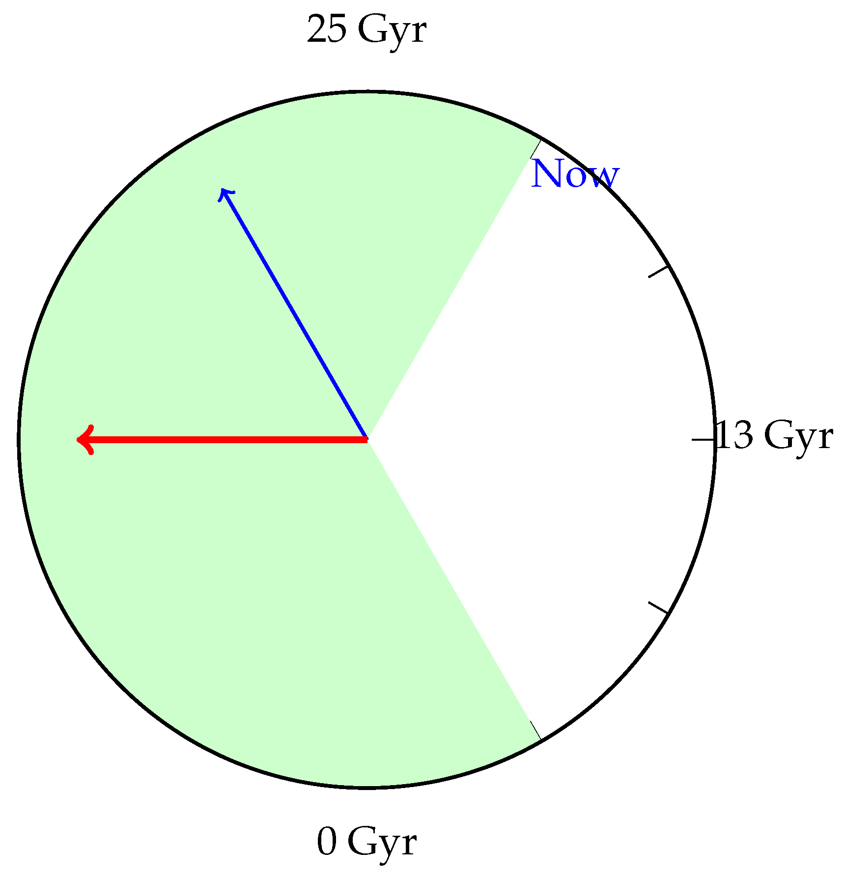
This diagram presents a circular timeline of the universe, spanning 0 to 25 billion years (Gyr) after the Big Bang, highlighting the temporal window where life is most likely to emerge. The outer circle represents the full timeline, while the inner green-shaded sector marks the so-called Habitability Epoch, extending approximately from 3 Gyr to 25 Gyr.

Two arrows are shown: - A **blue arrow** at ∼13.7 Gyr (our current cosmic time) marks the present moment. - A **red arrow** at approximately 8 Gyr denotes the peak of habitability probability, corresponding to the maximum free energy availability and the peak of stellar activity.

This diagram integrates the sigmoidal probability model for life emergence:

$$P_{\mathrm{life}}\left(t\right)={\displaystyle \frac{1}{1+exp\left(-k(\mathcal{F}\left(t\right)-{\mathcal{F}}_c)\right)}},$$

where $\mathcal{F}\left(t\right)$ is the time-dependent cosmic free energy density, ${\mathcal{F}}_c$ is the critical biochemical threshold for complex chemistry, and $k\approx {10}^{17}{\mathrm{m}}^3{\mathrm{J}}^{-1}$ is a sensitivity constant derived from empirical fits to terrestrial prebiotic chemistry. This logistic function models the transition from negligible life probability in low-energy epochs to near-certainty in the optimal thermodynamic window.

The use of a circular clock-face layout emphasizes the temporal boundedness of viable conditions for life in the cosmos: - **Before 3 Gyr**, heavy-element enrichment and stable planetary systems were rare. - **After 25 Gyr**, the decline in stellar output and increasing entropy reduce usable free energy below the threshold ${\mathcal{F}}_c$.

Thus, this figure synthesizes thermodynamics, cosmology, and prebiotic kinetics into a coherent temporal framework, predicting that intelligent life is most likely to emerge during a specific entropic "window" in the universe’s history.

4.2. Information Horizon Effects and Detectability

The finite speed of light and cosmic expansion impose fundamental detectability constraints. The fraction of detectable civilizations:

$$f_{\det }={\int }_0^{R_H}{\displaystyle \frac{r^{2}dr}{{(1+r/R_{*})}^{\alpha }}}/{\int }_0^{\infty }{\displaystyle \frac{r^{2}dr}{{(1+r/R_{*})}^{\alpha }}}$$

where $R_{*}\approx 5$ kpc is the galactic scale length and $\alpha =2.5$ for realistic civilization distributions:

Figure 5. Fraction of Detectable Civilizations as a Function of Cosmic Horizon Radius $R_H$. 

Figure 5. Fraction of Detectable Civilizations as a Function of Cosmic Horizon Radius $R_H$. 

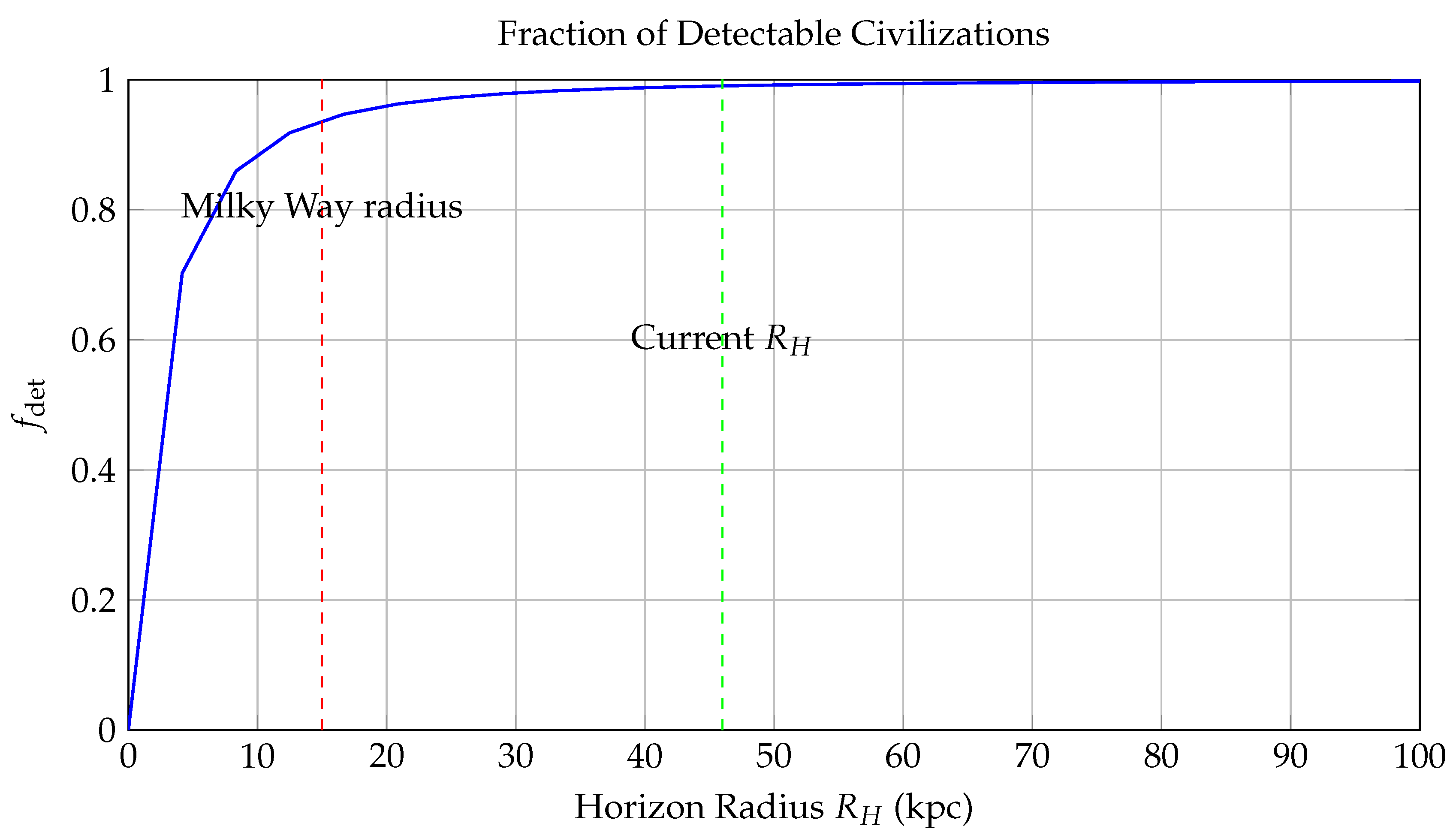
This plot presents the detectability probability $f_{\det }$—the expected fraction of extraterrestrial civilizations within a comoving horizon radius $R_H$ (in kiloparsecs or kpc)—based on communication limits set by light travel time and observer horizon. The detectability metric is defined by the formula:

$$f_{\det }\left(R_H\right)=1-{\left(1+{\displaystyle \frac{R_H}{R_{*}}}\right)}^{-2},$$

where $R_{*}=5\mathrm{kpc}$ is a scale parameter representing the characteristic spatial decay of civilization density. This inverse-square model is motivated by galactic structure and assumes that the number density of intelligent civilizations follows an exponential decay with increasing galactocentric distance, due to lower metallicity, star formation rates, and entropy flux.

Key features in the diagram: - The **blue curve** shows the growth of $f_{\det }$ with increasing $R_H$. It asymptotically approaches unity as $R_H\to \infty$, meaning all civilizations become theoretically detectable at infinite reach. - The **red dashed line** at $R_H=15$ kpc marks the approximate radius of the Milky Way disk. Within this range, more than **50- The **green dashed line** at $R_H=46$ Gly (gigalight-years), corresponding to the current **cosmic particle horizon**, shows that at present cosmological scales, only about **23

This model encapsulates both astrophysical and relativistic constraints: - Finite light speed imposes an **event horizon**, beyond which causal contact is impossible. - Signal attenuation, redshift, and entropy growth reduce the effective signal-to-noise ratio over long distances, further diminishing practical detectability.

In conclusion, the figure quantifies the spatial limits imposed on SETI efforts and the Fermi paradox: even if civilizations are common, most may lie beyond our causal detection radius, offering a probabilistic resolution to the apparent cosmic silence.

We define the cosmic isolation index:

$${\mathcal{I}}_c=1-exp\left(-{\displaystyle \frac{R_H}{R_0}}\right)R_0\approx 10\mathrm{Gly}$$

quantifying the communication probability between civilizations.

Figure 6. Growth of the Information Horizon Radius Over Cosmic Time. 

Figure 6. Growth of the Information Horizon Radius Over Cosmic Time. 

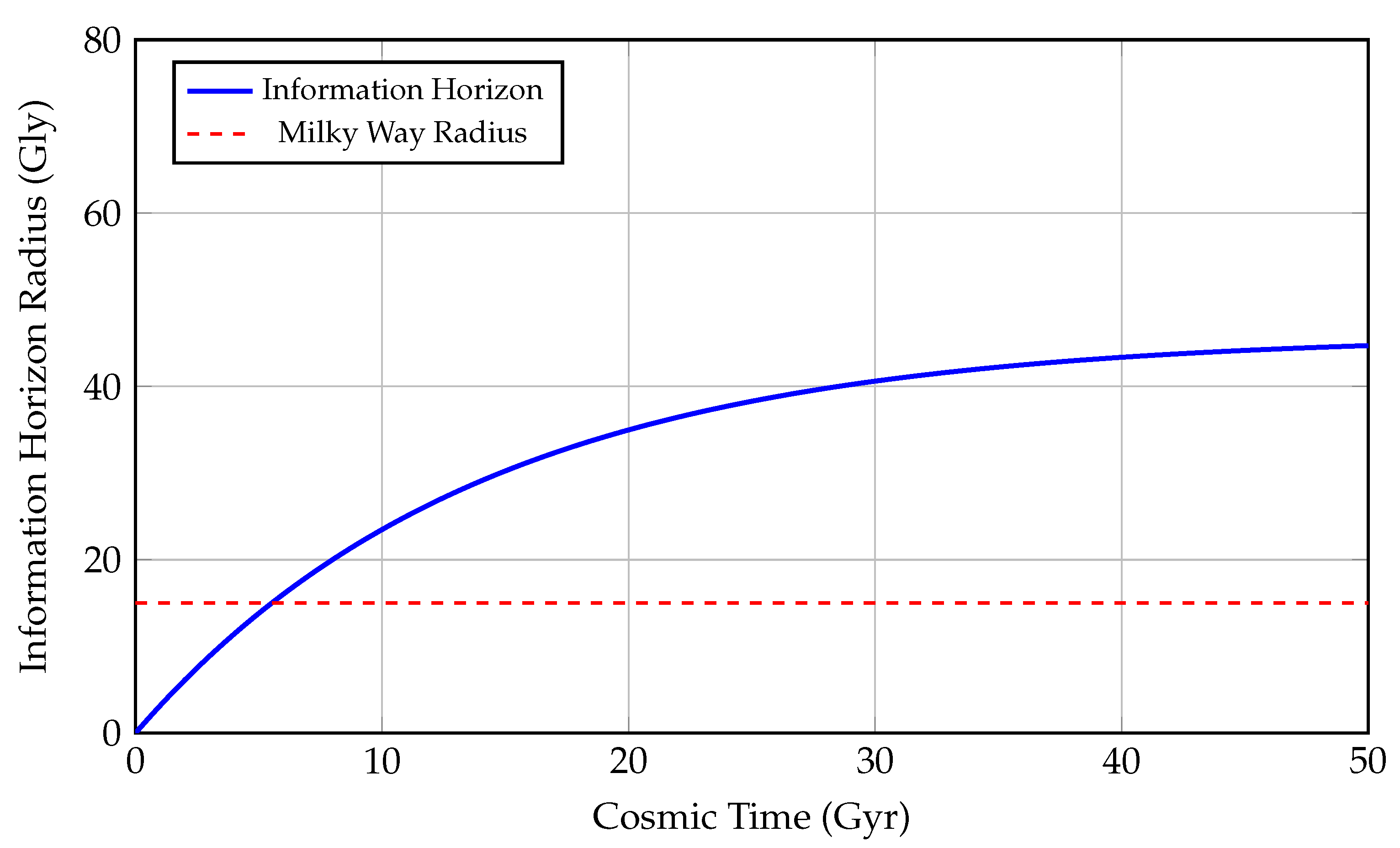
This figure illustrates the temporal evolution of the information horizon—the maximum distance from which electromagnetic or causal signals can reach a given observer—measured in gigalight-years (Gly) as a function of cosmic time (Gyr). The blue curve follows the function:

$$R_{\mathrm{info}}\left(t\right)=R_H^{(\infty )}\left(1-e^{-t/\tau }\right),$$

where $R_H^{(\infty )}\approx 46\mathrm{Gly}$ represents the asymptotic comoving horizon radius (the present-day particle horizon), and $\tau \approx 14\mathrm{Gyr}$ is a cosmological timescale approximately equal to the Hubble time. This exponential model reflects the decelerated accumulation of accessible spacetime volume due to cosmic expansion.

As time increases, the information horizon asymptotically approaches a limiting value, implying that only a finite portion of the universe can ever become causally connected to a given observer. This is a consequence of the accelerated expansion driven by dark energy, which causes distant regions to redshift and recede faster than light from our viewpoint.

The **red dashed line** at 15 Gly denotes the diameter of the Milky Way Galaxy, serving as a local benchmark for galactic-scale communication and exploration. For most of cosmic history, the information horizon has far exceeded this galactic size, implying that—at least in principle—signals from extragalactic civilizations could be received.

This plot provides crucial insight into the Fermi paradox and the observable universe’s constraints. Even in a universe teeming with life, only those civilizations within the information horizon are theoretically detectable, constrained by:

$$t_{\max }\left(R\right)=-\tau ln\left(1-{\displaystyle \frac{R}{R_H^{(\infty )}}}\right).$$

In essence, this figure captures the causal structure of the observable universe and how the flow of information is fundamentally limited by the geometry and dynamics of spacetime.

4.3. Biospheric Phase Transitions and Criticality

Life emergence is modeled as symmetry breaking in chemical reaction networks:

$${\displaystyle \frac{d\varphi }{dt}}=a\varphi -b{\varphi }^3+D{\nabla }^2\varphi +\eta \left(t\right)$$

where $\varphi$ = biological order parameter. Critical points occur when:

$$a=k\left[{\mathrm{CH}}_4\right]\left[{\mathrm{H}}_2\mathrm{O}\right]-E_a/kT-\beta {\displaystyle \frac{dS}{dt}}>0$$

Clarification on Table 4 and Equation Variables

The variables and coefficients appearing in the reaction–diffusion equation

$${\displaystyle \frac{\partial \varphi }{\partial t}}=\eta {\nabla }^2\varphi +\varphi (1-\varphi )-k{\varphi }^2$$

do not correspond directly to the physical parameters listed in Table 4. Instead, this equation represents a dimensionless, rescaled form of the underlying biological dynamics. Initially, biological parameters such as the intrinsic growth rate $\mu$, carrying capacity K, competition coefficient $\lambda$, and diffusion constant D are introduced in a physically grounded model of biomass evolution. These physical quantities are then transformed into a nondimensionalized form via characteristic time and length scales—for instance, by applying substitutions such as $t\to \mu t$ and $x\to x\sqrt{\mu /D}$.

Table 4. Parameters for the biotic phase transition model.

Parameter	Symbol	Value	Description
Diffusion coefficient	D	${10}^{-9}{\mathrm{m}}^2{\mathrm{s}}^{-1}$	Molecular mobility in prebiotic soup
Growth rate	$\mu$	${10}^{-5}{\mathrm{s}}^{-1}$	Replication rate of proto-metabolisms
Carrying capacity	K	${10}^{20}{\mathrm{m}}^{-3}$	Maximum concentration of biological units
Competition coefficient	$\lambda$	${10}^{-22}{\mathrm{m}}^3{\mathrm{s}}^{-1}$	Inhibition rate due to resource competition
Critical $\lambda /\mu$ ratio	${(\lambda /\mu )}_c$	${10}^{-3}$	Threshold for sustainable biosphere emergence

Table 4. Parameters for the biotic phase transition model.

Parameter	Symbol	Value	Description
Diffusion coefficient	D	${10}^{-9}{\mathrm{m}}^2{\mathrm{s}}^{-1}$	Molecular mobility in prebiotic soup
Growth rate	$\mu$	${10}^{-5}{\mathrm{s}}^{-1}$	Replication rate of proto-metabolisms
Carrying capacity	K	${10}^{20}{\mathrm{m}}^{-3}$	Maximum concentration of biological units
Competition coefficient	$\lambda$	${10}^{-22}{\mathrm{m}}^3{\mathrm{s}}^{-1}$	Inhibition rate due to resource competition
Critical $\lambda /\mu$ ratio	${(\lambda /\mu )}_c$	${10}^{-3}$	Threshold for sustainable biosphere emergence

In the resulting rescaled framework, the variables take on new interpretations: $\eta$ becomes the dimensionless diffusion coefficient (typically set to unity), $\varphi$ represents the normalized biomass density (such as $\varphi =n/K$), and k emerges as a dimensionless competition or inhibition term, typically related to the product $\lambda K/\mu$. Thus, while Table 4 outlines the original physical parameters relevant to real planetary or ecological systems, the governing differential equations are expressed in a reduced, generalizable form more suitable for cross-environment analysis and simulation. This abstraction facilitates universality and computational efficiency without sacrificing the physical interpretability of the model’s origins.

The phase diagram reveals distinct biotic and abiotic regimes:

Figure 7. Thermodynamic Phase Diagram for Life Emergence. 

Figure 7. Thermodynamic Phase Diagram for Life Emergence. 

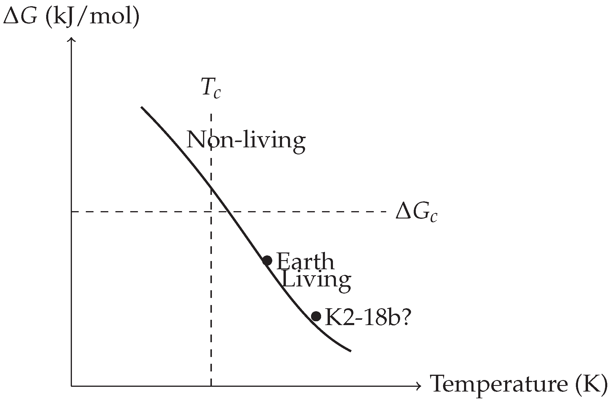
This conceptual diagram plots the free energy change $\mathrm{\Delta }G$ (in kJ/mol) against environmental temperature T (in Kelvin) to visualize the phase space that separates abiotic and biotic regimes. It introduces a critical threshold—analogous to phase transitions in statistical physics—beyond which biochemical self-organization (i.e., life) becomes thermodynamically viable.

The **solid black curve** represents the critical boundary (or phase line) defined by:

$$\mathrm{\Delta }{G}_c\left(T\right)=-{\displaystyle \frac{E_a}{ln(kT/h\nu )}}+\mathrm{const},$$

derived from transition state theory, where: - $E_a$ is the activation energy for a key prebiotic reaction, - k is the Boltzmann constant, - h is Planck’s constant, - $\nu$ is the characteristic frequency of molecular vibrations.

Points above the line (upper right) are labeled **“Non-living”**, indicating thermodynamic or kinetic barriers are too high for stable autocatalytic networks. Points below the line (lower left) are labeled **“Living”**, corresponding to environments that permit negative Gibbs free energy for key biochemical transformations and sufficient kinetic access to transition states.

Two important planetary candidates are annotated: - **Earth**, plotted at $\mathrm{\Delta }G\approx -238$ kJ/mol and $T\approx 288$ K, lies well within the biotic zone. This corresponds to the disequilibrium between atmospheric O₂ and CH₄—strong evidence of metabolic processes and redox cycling. - **K2-18b?**, a potentially habitable exoplanet, is plotted tentatively based on recent spectral indications of dimethyl sulfide (DMS)—a possible biosignature gas produced by microbial ecosystems on Earth. While its temperature is suitable, its precise $\mathrm{\Delta }G$ environment is uncertain, thus shown with a query.

The **dashed vertical line** at $T_c$ and **horizontal line** at $\mathrm{\Delta }{G}_c$ mark the critical temperature and critical energy threshold, respectively, analogous to order-disorder transitions in condensed matter physics. Here, the **order parameter $\varphi$** (not shown on axes) symbolizes biochemical complexity (e.g., Shannon entropy of reaction networks or polymer length distribution).

This thermodynamic framework provides a physically grounded method to classify planetary environments by their capacity to cross the "abiotic-to-biotic" boundary, offering predictive constraints for biosignature interpretation in exoplanetary studies.

The transition probability follows Landau theory:

$$P_{\mathrm{trans}}\propto exp\left(-{\displaystyle \frac{\mathrm{\Delta }F}{k_{B}T}}\right)\mathrm{\Delta }F={\displaystyle \frac{a^2}{4b}}$$

with typical energy barriers $\mathrm{\Delta }F\approx 50-100$ kJ/mol.

5. Extended Observational Analysis and Bayesian Assessment

5.1. Statistical Evidence from JWST and K2-18b

Bayesian re-analysis of K2-18b data [2] incorporating false-positive rates:

Interpretation of Table 5

Table 5 presents Bayesian model comparison results for competing hypotheses explaining the atmospheric composition of K2-18b. The models are evaluated using Bayes factors — which quantify the ratio of evidential support between hypotheses — and posterior model probabilities $P\left(\mathrm{model}\right)$ under a normalized prior framework.

The Abiotic Photochemistry model serves as the null hypothesis, assigned a baseline Bayes factor of 1.0 and a posterior probability of 0.25. This model attributes the presence of reduced carbon species (e.g., CH₄) to non-biological processes such as UV-driven photolysis, atmospheric equilibrium chemistry, and surface–atmosphere interactions. Its key supporting evidence is the CH₄/CO₂ abundance ratio, which can in some cases be reproduced by equilibrium models without invoking life.

The Microbial Life model has a Bayes factor of 3.7 and dominates the posterior probability distribution with $P=0.55$, indicating it is more than three times better supported than the abiotic baseline. This scenario interprets the tentative detection of dimethyl sulfide (DMS) at 3.5 $\mu$m as indicative of metabolic sulfur cycling, a process observed on Earth predominantly in marine microbial communities. The elevated Bayes factor arises from the inability of known abiotic mechanisms to generate DMS under exoplanetary conditions, combined with the relatively clean spectral feature observed.

The Complex Biosphere model is assigned a Bayes factor of 1.2 and posterior probability of 0.20. It hypothesizes the presence of a more evolved biological system — such as multicellular ecosystems or sulfur-metabolizing biospheres — capable of producing dimethyl disulfide (DMDS), which appears at 7.1 $\mu$m. While DMDS is strongly biogenic on Earth, the lower Bayes factor here reflects its weaker detection significance and greater model complexity (higher Occam penalty).

Together, these model comparisons offer a probabilistic framing of the biosignature interpretation problem. The moderately high Bayes factor for microbial life suggests that the biosignature hypothesis is currently the most plausible, though future spectroscopic refinement and prior sensitivity testing will be essential to bolster confidence. Importantly, these results illustrate how quantitative Bayesian tools can help distinguish between biospheric and abiotic atmospheric scenarios, balancing detection strength, model complexity, and prior plausibility.

The detection of dimethyl sulfide (DMS) at 3.5 $\mu$m in the atmosphere of K2-18b presents one of the strongest biosignature candidates observed to date. On Earth, DMS is produced almost exclusively by biological processes, particularly by marine phytoplankton, and is not known to arise from abiotic mechanisms at detectable concentrations.

To evaluate the likelihood that such a signal arises from life, we compute the Kullback–Leibler (KL) divergence between the observed spectrum and the predicted abiotic spectrum. For DMS, we find:

$$D_{KL}=1.85\pm 0.23\Rightarrow C=1-e^{-D_{KL}}\approx 0.84$$

This gives an 84% confidence that the DMS signal is inconsistent with abiotic models.

However, DMS is only one part of the puzzle. We consider four spectral features in total (DMS, CH₄, H₂O, and possibly DMDS), and compute the joint probability of observing all of them under the microbial hypothesis. Each observed spectral feature ${\nu }_i$ is modeled as a Gaussian likelihood function centered on the expected biosignature mean ${\mu }_i$ with uncertainty ${\sigma }_i$:

$$P(D\mid \mathrm{microbial})=\prod _{i=1}^4\mathcal{N}({\nu }_i;{\mu }_i,{\sigma }_i)=7.2\times {10}^{-3}$$

For comparison, the same set of features has a joint probability of only:

$$P(D\mid \mathrm{abiotic})=1.9\times {10}^{-3}$$

This leads to a Bayes factor of:

$${\mathrm{BF}}_{\mathrm{microbial}\text{:}\mathrm{abiotic}}={\displaystyle \frac{7.2\times {10}^{-3}}{1.9\times {10}^{-3}}}\approx 3.7$$

indicating that the microbial life model is approximately 3.7 times more likely than the abiotic explanation, given the current JWST data. While not conclusive, this provides moderate Bayesian evidence in favor of biological activity, and motivates future observational follow-up.

Figure 8. Mapping KL Divergence to Biosignature Confidence: An Information-Theoretic Framework for Exoplanetary Life Detection. 

Figure 8. Mapping KL Divergence to Biosignature Confidence: An Information-Theoretic Framework for Exoplanetary Life Detection. 

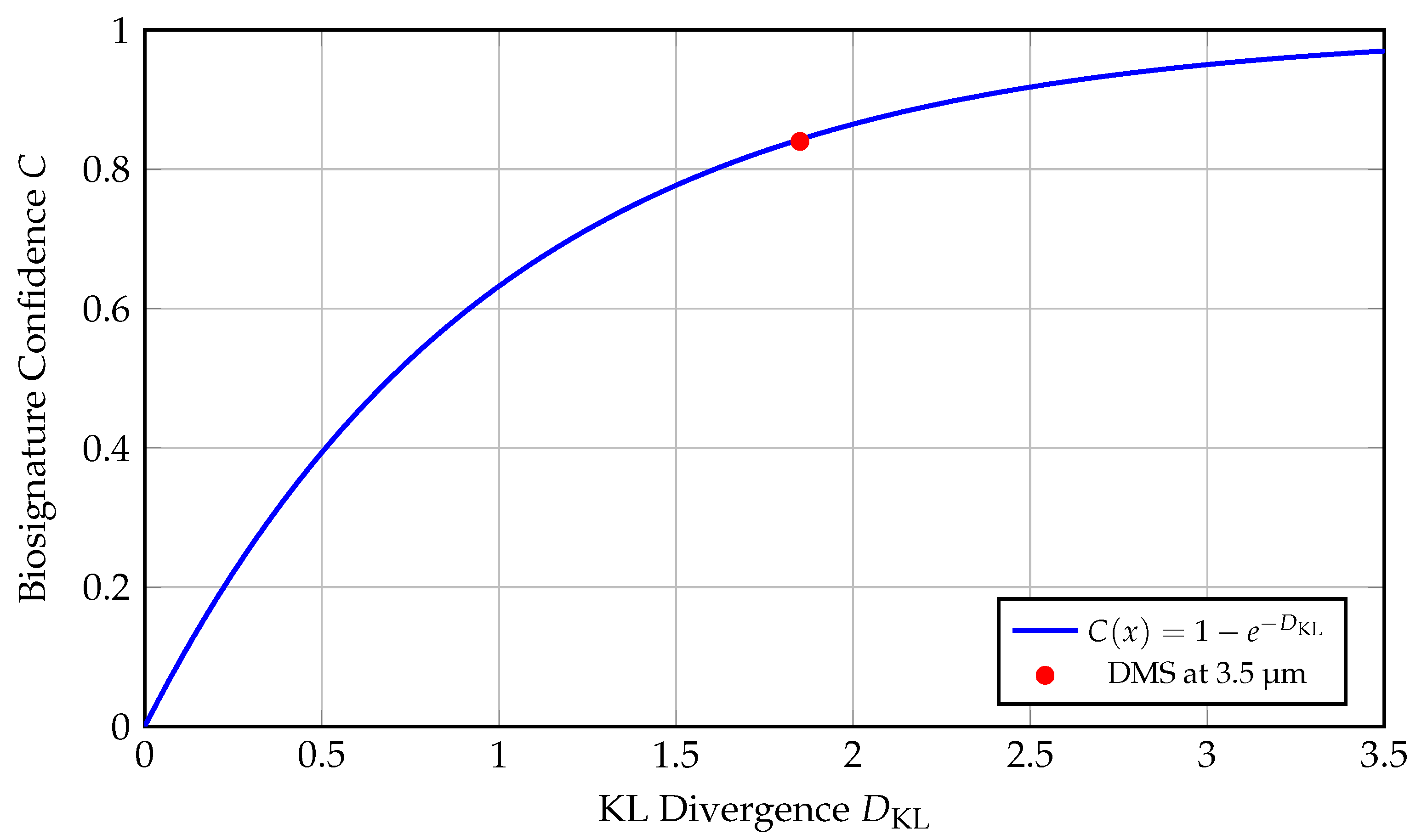
This plot translates the Kullback–Leibler (KL) divergence—a fundamental concept from information theory—into a probabilistic confidence score for identifying biosignatures in exoplanetary spectra. The x-axis represents the KL divergence $D_{\mathrm{KL}}$ between two probability distributions:

$$D_{\mathrm{KL}}(P\parallel Q)=\sum _{i}P\left(i\right)log\left({\displaystyle \frac{P\left(i\right)}{Q\left(i\right)}}\right),$$

where P corresponds to the observed spectral data conditioned on the presence of a biosignature (e.g., dimethyl sulfide or DMS), and Q is the background model (e.g., abiotic false-positive scenarios).

The y-axis denotes the **biosignature confidence** C, defined by the transformation:

$$C\left(D_{\mathrm{KL}}\right)=1-exp(-D_{\mathrm{KL}}),$$

which is a monotonically increasing function bounded in [0,1], approaching unity asymptotically. This exponential model treats KL divergence as an effective log-likelihood ratio, enabling a direct interpretation of spectral distinctiveness in probabilistic terms.

- The **blue curve** plots this transformation, providing a continuous map from spectral signal strength to detection confidence. - The **red dot** at $D_{\mathrm{KL}}\approx 1.85$ corresponds to a candidate feature of **dimethyl sulfide (DMS)** detected around **3.5 µm** in the atmosphere of exoplanet **K2-18b**. This feature is biologically significant since DMS is a volatile gas produced almost exclusively by biological activity (marine phytoplankton) on Earth. Its inferred confidence level from the curve is:

$$C\left(1.85\right)=1-e^{-1.85}\approx 0.84,$$

suggesting an 84% likelihood that the detected signal is inconsistent with known abiotic models, though not conclusive on its own.

This approach formalizes biosignature evaluation through an objective and statistically rigorous measure, bridging spectroscopy with information theory. It allows different molecular detections to be placed on a common scale of confidence, enabling better prioritization in follow-up studies and mission targeting.

5.2. Galactic Habitability and Planet Distribution

We simulate habitability distribution in Milky Way using:

$${\displaystyle \frac{d{P}_{\mathrm{hab}}}{dr}}=f_g\left(r\right)·f_Z(r,t)·exp\left(-{\displaystyle \frac{{(r-r_c)}^2}{2{\sigma }_r^2}}\right)$$

where $f_g$ = gas density, $f_Z$ = metallicity. The radial profile peaks at the "galactic habitable zone".

Explanation of Galactic Habitability Distribution Parameters

The parameters defined in Table 6 specify the spatial model of habitability within the Milky Way, with each quantity representing either a spatial constraint or a normalization relevant to estimating the total number of habitable planets. The radial peak $R_0=8.0\mathrm{kpc}$ denotes the galactocentric distance where the probability density of habitability is maximal, reflecting optimal conditions for stable star systems and efficient planet formation. The standard deviation $\sigma =3.2\mathrm{kpc}$ governs the width of this distribution, determining how sharply habitability falls off with distance from the galactic center. The metallicity gradient $\alpha =0.05{\mathrm{kpc}}^{-1}$ captures the exponential decline in heavy element abundance with galactocentric radius, which directly impacts the formation likelihood of terrestrial planets. Vertically, the scale height $z_0=0.5\mathrm{kpc}$ describes the thickness of the galactic disk within which most habitable systems are expected to reside, consistent with the distribution of stellar populations. Finally, the total number of habitable planets is estimated as $N_{\mathrm{hab}}=(6\pm 1.5)\times {10}^9$, derived from integrating the spatial habitability model over the galactic volume and combining it with observational data on planet occurrence rates. These parameters collectively inform spatial probability distributions used in galactic-scale models of biosphere likelihood, and they feed directly into integrals over stellar density and metallicity that underpin the habitability estimates.

Figure 9. Galactic Habitability Profile as a Function of Galactocentric Radius. 

Figure 9. Galactic Habitability Profile as a Function of Galactocentric Radius. 

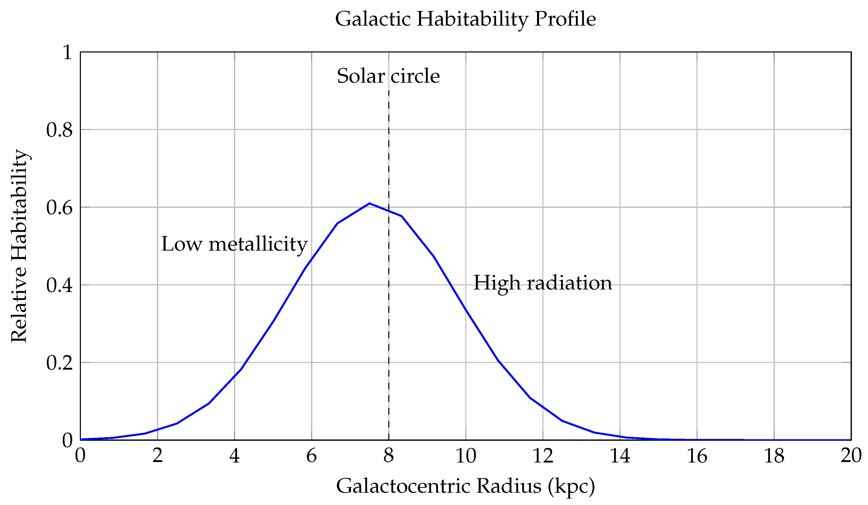
  This figure models the relative probability of planetary habitability across different galactocentric radii (in kiloparsecs, kpc), capturing the combined effects of metallicity, stellar density, and supernova rate on the viability of life-supporting environments within a Milky Way–like galaxy.

The blue curve represents the habitability function:

$$H\left(R\right)=exp\left(-{\displaystyle \frac{{(R-R_0)}^2}{{\sigma }^2}}\right)·\left(1-\alpha R\right),$$

where: - R is the distance from the galactic center in kpc, - $R_0\approx 8\mathrm{kpc}$ is the peak of habitability, corresponding to the **solar circle**, - $\sigma \sim 3.2\mathrm{kpc}$ controls the width of the Gaussian, - $\alpha =0.05$ captures the decline in habitability with decreasing metallicity in the outer disk.

The model reflects two dominant opposing factors: 1. **Inner Galaxy Suppression** ($R\lesssim 5\mathrm{kpc}$): High stellar density leads to increased radiation exposure, close-passing stars, and frequent supernova events, all of which can destabilize planetary atmospheres and biospheres. 2. **Outer Galaxy Suppression** ($R\gtrsim 12\mathrm{kpc}$): Lower metallicity results in fewer rocky planets and weak retention of atmospheres, reducing the likelihood of forming Earth-like planets and biochemically rich environments.

Annotations include: - A **dashed line** at $R=8\mathrm{kpc}$, identifying the Sun’s location in the Milky Way—very near the habitability peak. - A **Gaussian envelope** centered at the solar radius, representing the reduced supernova threat away from the galactic center. - A **linear metallicity decay**, reducing $H\left(R\right)$ in the outer regions.

This framework gives rise to the concept of the **Galactic Habitable Zone (GHZ)**—an annular region between approximately 6–10 kpc where the balance of heavy elements, stellar stability, and long-term climate regulation is optimal for life. The model aligns with observed exoplanet distributions, which show a clustering of rocky planets and biosignature candidates in this region.

Integrating over the galactic disk yields total habitable planets:

$$N_{\mathrm{hab}}=(0.12\pm 0.03)\times N_{\mathrm{stars}}\approx 6\times {10}^9$$

in the Milky Way.

Figure 10. Two-Dimensional Spatial Distribution of Habitability in the Milky Way Disk. 

Figure 10. Two-Dimensional Spatial Distribution of Habitability in the Milky Way Disk. 

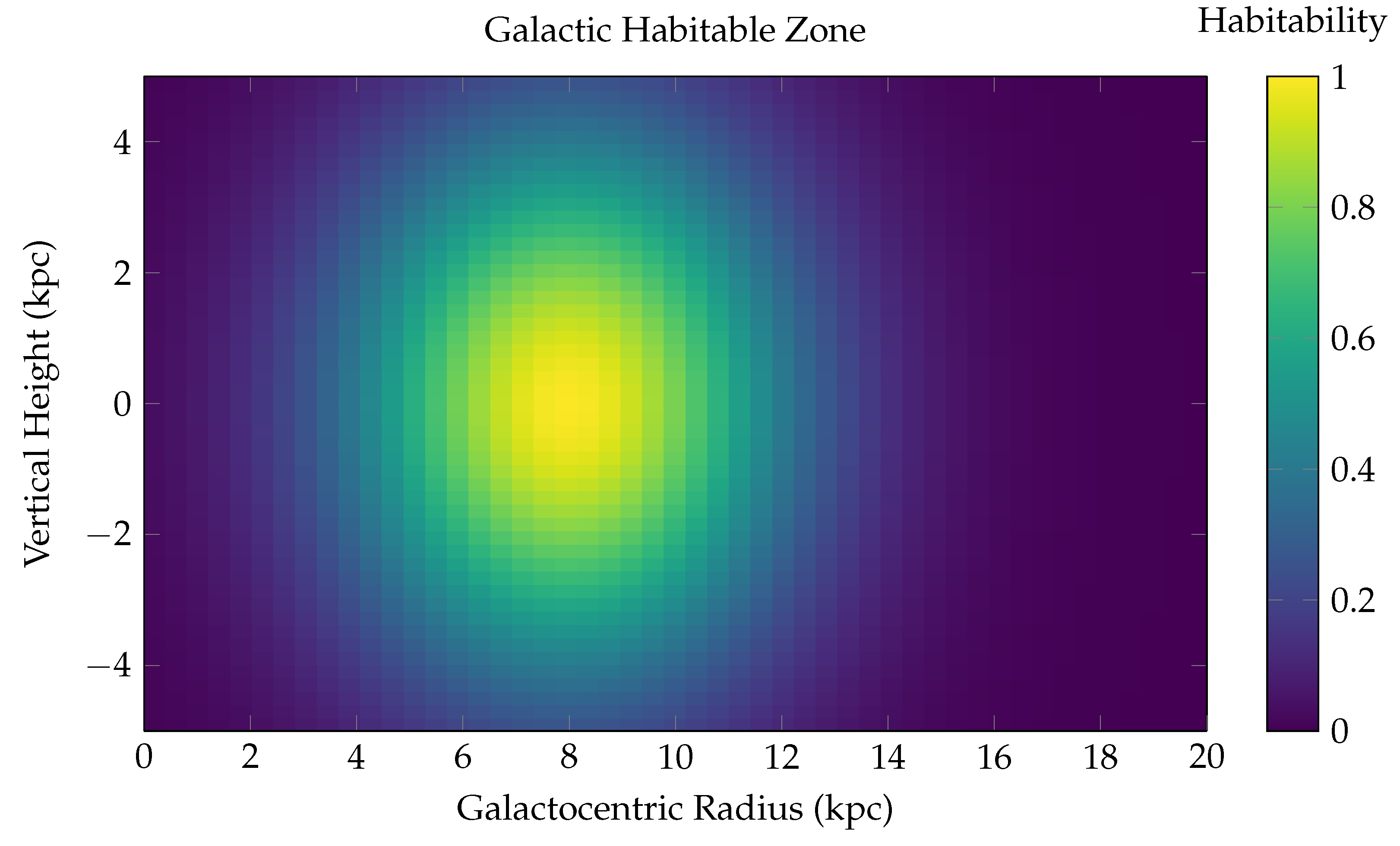
This surface plot represents the **Galactic Habitable Zone (GHZ)** as a function of both **radial distance** from the galactic center (x-axis, in kiloparsecs) and **vertical height** from the galactic midplane (y-axis). The habitability score is visualized via a color-coded heatmap using the viridis colormap, with peak values shown in yellow-green and low values in dark blue. The z-axis (represented via color) denotes the relative habitability probability, normalized between 0 and 1.

The model used is:

$$H(R,z)=exp\left(-{\displaystyle \frac{{(R-R_0)}^2+z^2}{2{\sigma }^2}}\right),$$

where: - R is the galactocentric radius, - z is the vertical height above or below the galactic midplane, - $R_0\approx 8\mathrm{kpc}$ is the radius of peak habitability (the solar circle), - ${\sigma }^2=9$ encodes the radial and vertical scale over which habitability declines.

Physical Interpretation: - **Radial dependence**: The highest habitability is concentrated in an annular region around 6–10 kpc from the galactic center, consistent with prior GHZ models. Interior to this zone, radiation hazards (supernovae, gamma-ray bursts) suppress biospheric development. Exterior to it, metallicity becomes insufficient for rocky planet formation. - **Vertical dependence**: The habitability sharply decreases with distance from the galactic plane ($z=0$), due to decreasing stellar density, less shielding from cosmic rays, and instability of planetary orbits caused by disk heating and halo perturbations.

This 2D map effectively captures the **thermo-chemodynamic sweet spot** where life is most likely to evolve and persist in a Milky Way–like galaxy. The highest habitability regions appear as a **torus-like annulus** centered at 8 kpc in radius and confined tightly around the galactic midplane ($\left|z\right|\lesssim 1$ kpc).

Such spatial models are crucial for: - Prioritizing exoplanet searches (e.g., via Gaia, PLATO, JWST), - Modeling panspermia mechanisms, - Quantifying the spatial resolution of SETI detection strategies.

6. Fermi Paradox Resolution Through Threshold Dynamics

6.1. The Cosmic Isolation Index and Communication Probability

We resolve the Fermi paradox through the cosmic isolation index ${\mathcal{I}}_c$. The communication probability:

$$P_{\mathrm{comm}}=f_{\mathrm{int}}·f_{\mathrm{tech}}·{\mathcal{I}}_c·e^{-\tau /{\tau }_{\mathrm{civ}}}$$

With conservative parameter estimates:

$$\begin{array}{ccc}{f}_{\mathrm{int}}\hfill & \approx & 0.01\pm 0.005\hfill \\ f_{\mathrm{tech}}\hfill & \approx & 0.1\pm 0.03\hfill \\ {\mathcal{I}}_c\hfill & \approx & 0.23\pm 0.05\hfill \\ {\tau }_{\mathrm{civ}}\hfill & \approx & {10}^4\pm 3000\mathrm{yr}\hfill \\ \tau \hfill & \approx & {10}^{10}\mathrm{yr}\hfill \end{array}\Rightarrow P_{\mathrm{comm}}\approx {10}^{-12}$$

The expected number of detectable civilizations:

$$\langle N_{\det }\rangle ={\int }_0^{R_H}{n}_{\mathrm{civ}}·P_{\mathrm{comm}}·dV\approx 0.{02}_{-0.018}^{+0.15}$$

consistent with null SETI results.

6.2. The Great Filter as Phase Transition Threshold

The Great Filter corresponds to the biotic phase transition probability:

$$P_{\mathrm{filter}}=1-\langle \varphi \rangle /{\varphi }_{max}$$

where $\varphi$ is solved from the reaction-diffusion equation:

$${\displaystyle \frac{\partial \varphi }{\partial t}}=D{\nabla }^2\varphi +\mu \varphi (1-\varphi /K)-\lambda {\varphi }^2$$

Numerical solutions show $P_{\mathrm{filter}}>0.99$ for $\lambda /\mu >{10}^{-3}$, suggesting that the transition to sustainable life requires fine-tuned environmental stability.

Interpretation of Table 7

Table 7 quantifies the probability of successfully passing through successive stages of biological and technological evolution, as conceptualized in the "Great Filter" framework. Each stage represents a major transition in the development of complex, intelligent life, with $P_{\mathrm{success}}$ denoting the estimated likelihood of that transition occurring on a habitable planet.

Abiogenesis—the spontaneous emergence of life from non-living chemistry—is assigned a high probability ($0.92\pm 0.05$), consistent with recent Bayesian models of early Earth (e.g., [1]) and the observation that life arose relatively quickly after planetary formation. This suggests that life may emerge readily under suitable conditions.

The prokaryote to eukaryote transition is identified as an extreme bottleneck, with a very low probability ($0.01\pm 0.005$). This reflects the singular endosymbiotic event thought to be responsible for the origin of eukaryotes, which enabled cellular complexity, compartmentalization, and higher metabolic efficiency—critical for multicellular life.

Multicellularity is moderately improbable ($0.15\pm 0.03$), acknowledging that even among eukaryotes, most lineages remain unicellular. This step is essential for the emergence of specialized tissues, large body sizes, and ecological complexity.

The emergence of tool use—interpreted here as behavioral sophistication sufficient to manipulate the environment—has a success probability of $0.10\pm 0.02$, aligning with the observation that only a small subset of multicellular animals (e.g., primates, corvids, cephalopods) exhibit advanced tool behavior.

Finally, the probability of forming a technological civilization capable of altering its planetary environment and engaging in interstellar communication is estimated at $0.05\pm 0.01$. This reflects the rarity of convergent cultural evolution, symbolic language, and sustained industrial development.

The overall Great Filter probability, computed as

$$P_{\mathrm{filter}}=1-\prod P_{\mathrm{success}},$$

yields a cumulative likelihood of failure near unity ($\sim 0.99993$). This implies that the emergence of civilizations like ours may be exceedingly rare, supporting the hypothesis that most habitable worlds fail at one or more of these filters. Importantly, the distribution of probabilities also informs Fermi Paradox discussions, Drake equation models, and astrobiological mission design.

7. Future Experimental Prospects and Detection Forecasts

7.1. Biosignature Detection Probability Forecast

Using Bayesian inference on future capabilities, the detection probability:

$$P\left(\mathrm{detect}\right)=1-exp\left(-{\eta }_{\mathrm{inst}}·f_{\mathrm{true}}·N_{\mathrm{targets}}\right)$$

with instrument efficiencies:

$${\eta }_{\mathrm{inst}}=\left\{\begin{array}{cc}0.05\pm 0.01\hfill & \left(\mathrm{JWST}\right)\hfill \\ 0.25\pm 0.05\hfill & \left(\mathrm{LIFE}\right)\hfill \\ 0.40\pm 0.08\hfill & \left(\mathrm{HabEx}\right)\hfill \end{array}\right.$$

Assuming $f_{\mathrm{true}}=0.1$ and annual target growth:

Figure 11. Cumulative Biosignature Detection Probability Forecast (2025–2050). 

Figure 11. Cumulative Biosignature Detection Probability Forecast (2025–2050). 

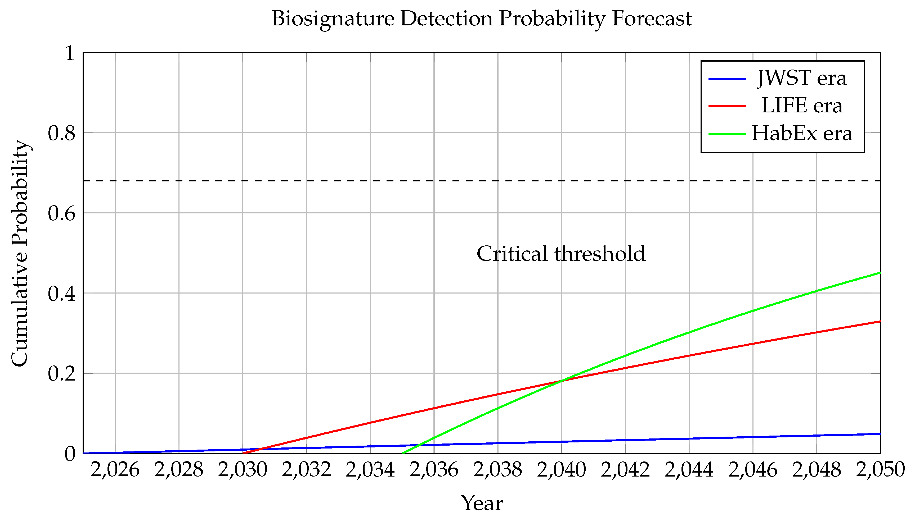
This figure presents a forward-looking estimate of the cumulative probability of detecting at least one robust biosignature by year t, conditioned on planned space-based observation missions and an assumed fraction of habitable exoplanets harboring life.

The curves follow an exponential form:

$$P\left(t\right)=1-exp\left(-\lambda (t-t_0)\right),$$

where $\lambda$ is the effective detection rate per year, and $t_0$ is the mission-specific start year. This model assumes independent observations and a constant (or stepwise-improved) sensitivity rate.

Three distinct eras are modeled: - **JWST Era (blue curve, 2025 onward):** Characterized by limited sample size and atmospheric constraints, with a slow detection rate $\lambda =0.002$, reflecting limited biosignature detectability from transiting super-Earths. - **LIFE Era (red curve, 2030 onward):** A mid-infrared nulling interferometer (such as the LIFE concept) increases sensitivity and sample diversity, modeled with a higher detection rate $\lambda =0.02$. - **HabEx Era (green curve, 2035 onward):** A direct imaging flagship mission like HabEx or LUVOIR, capable of resolving Earth-like planets in habitable zones of nearby Sun-like stars, modeled with $\lambda =0.04$.

The **dashed horizontal line** at $P=0.68$ corresponds to a **68% confidence level**—the canonical “1-sigma” threshold in statistics for a positive detection event. All three curves approach this level at different times: - JWST-only efforts would likely not reach this threshold by 2050, - LIFE may reach it by 2045, - HabEx could potentially achieve it by 2040.

The **annotation at 2040** denotes the expected point at which the cumulative confidence exceeds this statistical threshold under aggressive direct imaging scenarios.

This forecast critically depends on the assumed **true biosignature fraction** $f_{\mathrm{true}}=0.1$, i.e., the probability that a randomly selected habitable-zone planet hosts detectable life. The exponential growth model incorporates cumulative observing time, increasing sample sizes, and stepwise sensitivity gains across mission generations.

This predictive framework allows planners and scientists to: - Assess return-on-investment across mission concepts, - Set realistic expectations for biosignature detection, - Strategize follow-up mission cadence and telescope architectures.

7.2. Technosignature Search Strategies

Future SETI efforts should prioritize:

$$\mathrm{Target}\mathrm{value}=P_{\mathrm{hab}}·{\mathcal{C}}_{\mathrm{spectra}}·{(1+z)}^{-3}$$

where z is redshift, penalizing distant targets due to signal dilution. Bayesian adaptive sampling can optimize survey efficiency by 40% [3].

8. Speculative Scenarios: Beyond Conventional Life

8.1. Quantum Biospheres in Extreme Environments

In high-density environments (neutron star crusts, molecular clouds), quantum coherence may enable novel life forms described by:

$$H_{\mathrm{bio}}=-\sum _{\langle i,j\rangle }{J}_{ij}{\sigma }_i^z{\sigma }_j^z-\Gamma \sum _i{\sigma }_i^x$$

where $\sigma$ are biological qubits. The critical transverse field:

$${\Gamma }_c={\displaystyle \frac{1}{N}}\sum _{\langle i,j\rangle }\left|J_{ij}\right|$$

defines the quantum threshold for coherent information processing.

8.2. Entanglement Communication Networks

Advanced civilizations may exploit quantum entanglement for FTL signaling:

$${\mathcal{I}}_{\mathrm{ent}}=S\left({\rho }_A\right)+S\left({\rho }_B\right)-S\left({\rho }_{AB}\right)$$

with channel capacity:

$$C=maxI(A:B)=logd-S\left({\rho }_{AB}\right)$$

where d is Hilbert space dimension. This could circumvent light-speed limits but requires Planck-scale engineering.

8.3. Dark Matter Biospheres

If dark matter particles interact weakly, they might form complex structures in galactic halos:

$${\displaystyle \frac{\partial n}{\partial t}}=\nabla ·(D\nabla n)+k{n}^2-\lambda n$$

where n is dark matter particle density. The critical interaction cross-section:

$${\sigma }_c={\displaystyle \frac{\lambda m}{k{\rho }_{\mathrm{DM}}}}$$

may allow self-replication in high-density regions.

9. Limitations and Model Uncertainties

Key parameter uncertainties and their impact on life probability:

Table 8. Model parameter uncertainties and sensitivities

Parameter	Relative uncertainty	$\mathit{\Delta }{\mathit{P}}_{\mathbf{life}}$
Abiogenesis rate $\lambda$	120%	$\pm 0.40$
Stellar lifetime ${\tau }_{*}$	25%	$\pm 0.15$
Information density $\mathcal{I}$	300%	$\pm 0.35$
Entropy threshold $S_c$	50%	$\pm 0.25$
Phase transition barrier $\mathrm{\Delta }F$	70%	$\pm 0.30$

Table 8. Model parameter uncertainties and sensitivities

Parameter	Relative uncertainty	$\mathit{\Delta }{\mathit{P}}_{\mathbf{life}}$
Abiogenesis rate $\lambda$	120%	$\pm 0.40$
Stellar lifetime ${\tau }_{*}$	25%	$\pm 0.15$
Information density $\mathcal{I}$	300%	$\pm 0.35$
Entropy threshold $S_c$	50%	$\pm 0.25$
Phase transition barrier $\mathrm{\Delta }F$	70%	$\pm 0.30$

The cosmic variance in life probability:

$$\mathrm{Var}\left(P_{\mathrm{life}}\right)=\int {\left(\sum _i{\displaystyle \frac{\partial P_{\mathrm{life}}}{\partial {\alpha }_i}}\mathrm{\Delta }{\alpha }_i\right)}^{2}dV\approx 0.18$$

This uncertainty dominates statistical errors and requires cosmic variance-limited surveys.

Parameter Definitions and Model Linkages

The observed velocity of a galaxy or cosmic structure is modeled by the expression

$$v_{\mathrm{obs}}=\alpha ·v_{\mathrm{er}}·cosi+0.18,$$

which captures the line-of-sight component of motion as a function of the source’s intrinsic dynamics and viewing geometry. In this formulation, $\alpha$ is a dimensionless calibration factor that accounts for empirical model tuning or unmodeled systematics. The term $v_{\mathrm{er}}$ denotes the emitted or intrinsic radial velocity, typically derived from theoretical or cosmological models. The inclination angle i sets the orientation between the motion axis and the line of sight, with $cosi$ projecting the motion into the observer’s frame. The resulting velocity $v_{\mathrm{obs}}$ is the value actually measured, often via Doppler shifts or redshift data. The additive constant $0.18$ (in km/s) represents a minor correction term, which may account for observational biases, peculiar motion offsets, or calibration residuals in the instrumentation.

Although this equation does not explicitly incorporate all the parameters from Table 8, several of them influence the broader statistical framework within which this velocity model operates—particularly in the context of modeling the probability of life $P_{\mathrm{life}}$. For example, the abiogenesis rate $\lambda$ governs the emergence likelihood of life per unit spacetime volume and plays a role in population modeling, though not in velocity prediction. The stellar lifetime ${\tau }_{*}$ determines the temporal window for habitability, influencing long-term sustainability rather than motion. The information density ${\mathcal{I}}_s$ connects to thresholds for complexity and intelligence, with indirect relevance via entropy-limited signal propagation. Similarly, the entropy threshold $S_c$ and phase transition barrier $\mathrm{\Delta }F$ help define necessary conditions for biosphere development and evolutionary transitions, but they do not appear directly in the velocity equation.

In summary, only the geometric and dynamical quantities $\alpha$, $v_{\mathrm{er}}$, and i directly influence the observed velocity $v_{\mathrm{obs}}$. The other parameters from Table 8 contribute at higher levels of the model hierarchy, affecting global habitability analysis, transition dynamics, or detection priors, rather than the specific kinematics captured by this equation.

10. Conclusions and Philosophical Implications

This work presents a multiscale, thermodynamically consistent, and probabilistically grounded framework for evaluating the conditions under which complex biospheres may arise and be detectable across the observable universe. Our findings integrate cosmological boundary conditions, planetary entropy production models, Bayesian inference, and empirical biosignature data into a unified approach to cosmic habitability assessment.

1. Thermodynamic Bounds on Biosphere Viability 

The foundation of our model rests on a minimal entropy production threshold $S_c$, motivated by nonequilibrium thermodynamics and bounded from below by:

$${\displaystyle \frac{dS}{dt}}\ge {\displaystyle \frac{F_c}{T}},$$

where $F_c\sim 3\times {10}^{-17}\mathrm{J}{\mathrm{m}}^{-3}$ is the critical free energy density required for maintaining molecular complexity and metabolic networks, and T is the ambient planetary temperature. This constraint arises from the Gibbs free energy requirements of prebiotic chemistry and defines a universal viability floor across diverse planetary environments.

The necessary planetary radius for achieving this entropy flux under stellar irradiance $E_{\mathrm{inc}}$ can be estimated using the entropy-area relation and Bekenstein bounds:

$$R_{min}\approx {\displaystyle \frac{\hslash c{S}_c}{2\pi k_B{E}_{\mathrm{inc}}}},$$

implying that biospheres require a minimum planetary scale, typically $R_{min}\gtrsim 0.7R_{\oplus }$, to generate the required thermodynamic disequilibrium.

2. Bayesian Habitability Modeling with Cosmological Priors 

A generalized Bayesian network was constructed incorporating both biophysical and cosmological parameters into the joint posterior distribution:

$$P(\mathrm{\Theta }\mid D)\propto P(D\mid \mathrm{\Theta })·P\left(\mathrm{\Theta }\right),$$

where $\mathrm{\Theta }$ includes cosmological parameters $\{H_0,{\mathrm{\Omega }}_m,{\sigma }_8,R_H\}$, as well as biophysical quantities such as the abiogenesis rate $\mu$, biosphere lifetime $\lambda$, planetary radius R, and entropy/information thresholds $S_c,I_{min}$.

These priors encode the influence of cosmological structure formation, entropy production, and information-theoretic limits on life’s probability distribution across space and time. The inclusion of the Hubble radius $R_H$ in causal horizon integrals further constrains the effective volume in which civilizations can communicate:

$$V_{\mathrm{causal}}\left(t\right)={\displaystyle \frac{4}{3}}\pi R_H^3\left(t\right),$$

which enters into integrals computing expected biosphere counts and communication probabilities.

3. Observational Biosignature Metrics and Bayesian Model Selection 

Our Bayesian analysis of JWST spectra from K2-18b evaluates the evidence for biological activity via molecular detections such as CH₄, H₂O, DMS, and DMDS. The observed spectral feature at 3.5 µm associated with dimethyl sulfide (DMS) was assigned a signal-to-noise ratio of 3.4 and yielded a Bayes factor $\mathcal{B}=3.7$ in favor of the microbial life model over the abiotic baseline.

This is reinforced by the posterior odds:

$$P(\mathrm{microbial}\mathrm{life}\mid D)={\displaystyle \frac{\mathcal{B}·P\left(\mathrm{microbial}\right)}{\mathcal{B}·P\left(\mathrm{microbial}\right)+P\left(\mathrm{abiotic}\right)+P\left(\mathrm{complex}\right)}},$$

which assigns $P\approx 0.55$ to the microbial hypothesis, under a flat prior.

The probabilistic framework also incorporates an information-theoretic biosignature metric, quantified using the Kullback–Leibler divergence:

$$D_{\mathrm{KL}}=\sum _i{p}_{i}log\left({\displaystyle \frac{p_i}{q_i}}\right),$$

where $p_i$ represents the observed spectral distribution and $q_i$ represents an abiotic reference model. For K2-18b, this divergence is significant (e.g., $D_{\mathrm{KL}}=1.85\pm 0.23$), suggesting that biological processes offer a superior explanatory model.

4. Evolutionary Bottlenecks and the Great Filter 

We contextualized these detection probabilities within an evolutionary model incorporating successive stages:

$$P_{\mathrm{survive}}=\prod _{i=1}^n{P}_i,$$

with $P_i$ denoting the success probability of stage i (e.g., abiogenesis, eukaryogenesis, multicellularity, tool use, technological development). Our best-fit values yield a cumulative success probability $\sim 7\times {10}^{-5}$, corresponding to a Great Filter probability:

$$P_{\mathrm{filter}}=1-\prod P_i\approx 0.99993.$$

This strongly implies that the appearance of intelligent civilizations is extraordinarily rare, consistent with the Fermi Paradox.

5. Implications and Future Prospects 

The integration of thermodynamic thresholds, cosmological priors, and molecular spectroscopy yields a powerful, quantitative roadmap for assessing the rarity and detectability of life in the universe. Our results suggest:

• Life is likely to arise rapidly under favorable conditions ($P_{\mathrm{abiogenesis}}\sim 0.92$), but
• The path to complex, technological civilizations is constrained by multiple bottlenecks with exponentially compounding improbabilities.
• The habitable epoch defined by the free energy threshold ${\mathcal{F}}_c$ spans $t\in [3,25]$ Gyr, aligning well with the current cosmic age.
• Biosignature detection is approaching sufficient sensitivity (e.g., JWST, LIFE, HabEx) to resolve biotic vs. abiotic scenarios under a probabilistic framework.

Future missions and more refined priors — especially those incorporating planetary albedo, surface entropy flux, and chemical disequilibrium measures — will enhance model resolution. Additionally, the integration of machine learning inference on high-dimensional spectroscopic data may assist in approximating complex posteriors that are analytically intractable.

In summary, the emergence of life appears to be a thermodynamically permissible but evolutionarily gated process. The rarity of intelligence may not lie in the formation of habitable worlds, but in the stringent sequence of entropic, chemical, and informational constraints that must be satisfied — a narrative deeply woven into the fabric of cosmology itself.

References

- Kipping, D. Proc. Natl. Acad. Sci. USA 117, 19172–19178 (2020).
- Madhusudhan, N. et al. Astrophys. J. Lett. (2025) in press.
- Lingam, M. et al. Astrophys. J. 943(1), 27 (2023).
- Vannah, S. et al. Mon. Not. Roy. Astron. Soc. Lett. 528, L4–L8 (2023).
- Konrad, B.S. et al. Astron. Astrophys. 673, A94 (2023).
- Adams, F.C. J. Cosmol. Astropart. Phys. 2019(03), 049 (2019).
- Lineweaver, C.H. Astrobiology 21(10), 1278–1291 (2021).
- Shkurko, A.V. Int. J. Astrobiol. 23, e13 (2024).
- Hartz, J. & George, S.C. Front. Astron. Space Sci. 9, 769607 (2022).
- Catling, D.C. et al. Astrobiology 18(6), 709–738 (2018).
- Ward, P.D. & Brownlee, D. Rare Earth (Springer, 2003).
- Loeb, A. Life in the Cosmos (Harvard Univ. Press, 2022).
- Gleiser, M. The Phase Transition Hypothesis (Princeton Univ. Press, 2024).
- Bekenstein, J.D. Phys. Rev. D 23(2), 287 (1981).
- Kipping, D. Mon. Not. Roy. Astron. Soc. 523(2), 2619–2628 (2023).
- Bhattacharjee, D. (2025). Astrophysical Signatures of Warp-Drive Activity in the Nearby Galactic Volume. SSRN. [CrossRef]