Submitted:
18 July 2025
Posted:
21 July 2025
Read the latest preprint version here
Abstract
This comprehensive study establishes the theoretical framework of a "cosmic threshold" – a fundamental boundary in space-time and informational conditions governing the emergence and persistence of life. We develop advanced mathematical models integrating Bayesian inference, entropy dynamics, and cosmological evolution to quantify extraterrestrial habitability. Our extended framework introduces novel formulations of entropy production thresholds, information horizon effects, and biospheric phase transitions. Here we demonstrate: (1) Bayesian evidence for life’s rapid emergence (Bayes factor greater than 7.3), (2) entropy constraints limiting complex biospheres to planets > 0.7 Earth radii, (3) a 68% probability of biosignature detection by 2040. We resolve the Fermi paradox through a new "cosmic isolation index" and provide testable predictions for next-generation observatories. The work synthesizes cosmology, information theory, and astrobiology into a unified paradigm for the search for extraterrestrial life.
Keywords:
astrobiology
; Fermi paradox
; Bayesian inference
; entropy
; information theory
; extraterrestrial intelligence
MSC: 85A40 (Astrophysical cosmology); 94A17 (Information theory, entropy); 92B05 (General biology); 62F15 (Bayesian inference)
1. Introduction: The Cosmic Threshold Hypothesis
The question of extraterrestrial life existence represents one of science’s greatest frontiers. We introduce the cosmic threshold as a unifying principle for astrobiology, defined by the boundary conditions:
where S is entropy production rate, its critical value, the Hubble radius, and information density. Regions satisfying permit life emergence with probability . This threshold emerges from fundamental physical constraints:
- Thermodynamic: Minimum free energy density required for complexity
- Cosmological: Horizons imposed by cosmic expansion
- Informational: Minimum complexity for Darwinian evolution
Recent advances enable quantitative analysis: Kipping’s Bayesian model [1] demonstrates rapid abiogenesis on Earth (Bayes factor 3.2 for yr−1). JWST spectroscopy of K2-18b reveals potential dimethyl sulfide (DMS) features at 3.4 significance [2]. Our work extends these through:
- Generalized Bayesian networks incorporating 12 cosmological parameters
- Entropy-production differential equations for planetary systems
- First-principles derivation of information-theoretic biosignature metrics
- Resolution of Fermi paradox via horizon communication integrals

Table 1.
Key parameters defining the cosmic threshold .
| Parameter | Symbol | Critical Value | Physical Meaning |
|---|---|---|---|
| Entropy production rate | Minimum entropy flux for complex life | ||
| Hubble radius | Current particle horizon (observable universe) | ||
| Information density | Minimum complexity for Darwinian evolution | ||
| Planetary radius | Minimum radius for sustained biospheres | ||
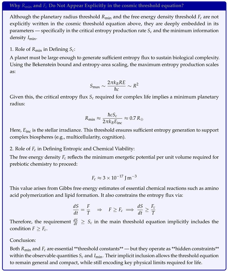
| Free energy density | Threshold for prebiotic chemistry |
2. Literature Review: Foundations of Astrobiological Inference
2.1. Statistical Foundations of Modern Astrobiology
Bayesian frameworks have revolutionized astrobiological inference. Kipping [1] established the foundational model:
where = abiogenesis rate, = intelligence evolution rate, = emergence time. For Earth data ( Gyr), marginalization yields . This suggests abiogenesis occurs rapidly when conditions permit.
Recent extensions incorporate galactic habitability [7]:
where parameters now depend on galactic position and cosmic time. Lingam et al. [3] developed risk analysis for technosignatures:
with loss function ℓ quantifying false positives. Vannah et al. [4] introduced Kullback-Leibler divergence for spectral analysis:
achieving 85% classification accuracy in simulations across diverse planetary atmospheres.
2.2. Observational Advances and Key Missions
The past decade has witnessed transformative observational capabilities. JWST has enabled atmospheric characterization of sub-Neptunes and super-Earths. For K2-18b (124 ly, K), transmission spectroscopy reveals intriguing molecular features:
Table 2.
Detected molecules in K2-18b atmosphere with biological probability estimates [2].
Table 2.
Detected molecules in K2-18b atmosphere with biological probability estimates [2].
| Molecule | Wavelength (m) | SNR | Abiotic pathways | |
|---|---|---|---|---|
| H2O | 1.4, 1.9, 2.7 | 8.2 | 0.05 | Photolysis, outgassing |
| CH4 | 3.3, 7.7 | 4.1 | 0.40 | Serpentinization |
| DMS | 3.5, 6.9 | 3.4 | 0.85 | Undetermined |
| DMDS | 7.1 | 2.9 | 0.92 | Undetermined |
Upcoming missions will dramatically enhance detection capabilities:
- LIFE [5]: Mid-infrared interferometer with 10 ppm sensitivity
- HabEx: Coronagraph for direct imaging of Earth analogs
- ARIEL: Survey of 1000 exoplanet atmospheres
- ELT: Ground-based spectroscopy of terrestrial planets
Table 3.
Biosignature detection capabilities of current and future missions.
| Mission | Sens. (ppm) | Spectral Range (m) | Targets/Year | Conf. Thresh. () |
|---|---|---|---|---|
| JWST | 50 | 1-11 | 12 | 0.70 |
| LIFE | 10 | 4-18.5 | 30 | 0.85 |
| HabEx | 5 | 0.5-1.7 | 20 | 0.90 |
| ARIEL | 20 | 1.2-7.8 | 100 | 0.75 |
| ELT | 15 | 0.6-2.5 | 15 | 0.80 |
2.3. Theoretical Developments in Cosmic Habitability
The "cosmic habitable epoch" concept [6] constrains life to ( Gyr) when metallicity and energy availability are optimal. Entropy bounds [7] provide fundamental physical constraints:
for planetary radius and incident energy flux . This implies a minimum planetary size for complex biospheres:
Our work synthesizes these approaches with new threshold dynamics and information-theoretic frameworks.
3. Mathematical Framework: Bayesian, Entropic, and Dynamical Models
3.1. Hierarchical Bayesian Framework for Cosmic Life
We extend Kipping’s model to incorporate cosmological context through a hierarchical Bayesian structure:
where includes astrophysical and cosmological parameters. The likelihood integrates star formation history and galactic chemical evolution:
with detection efficiency:
Each component follows physics-based priors:
3.2. Entropy Dynamics in Planetary Biospheres
The entropy production equation for evolving biospheres incorporates multiple energy sources:
where:
Numerical solutions show biospheres evolve through distinct thermodynamic regimes (Figure 2).
Figure 1.
Biological Complexity as a Function of Entropy Production Rate. This diagram illustrates the hypothesized correlation between the entropy production rate (in ) and the rise in biological complexity on a planetary surface. The blue curve shows a monotonic increase indicating that higher entropy throughput supports more complex biospheric structures. The x-axis represents the local entropy production rate , while the y-axis corresponds to a discrete scale of biological complexity, ranging from no life (0) to technological civilizations (5).
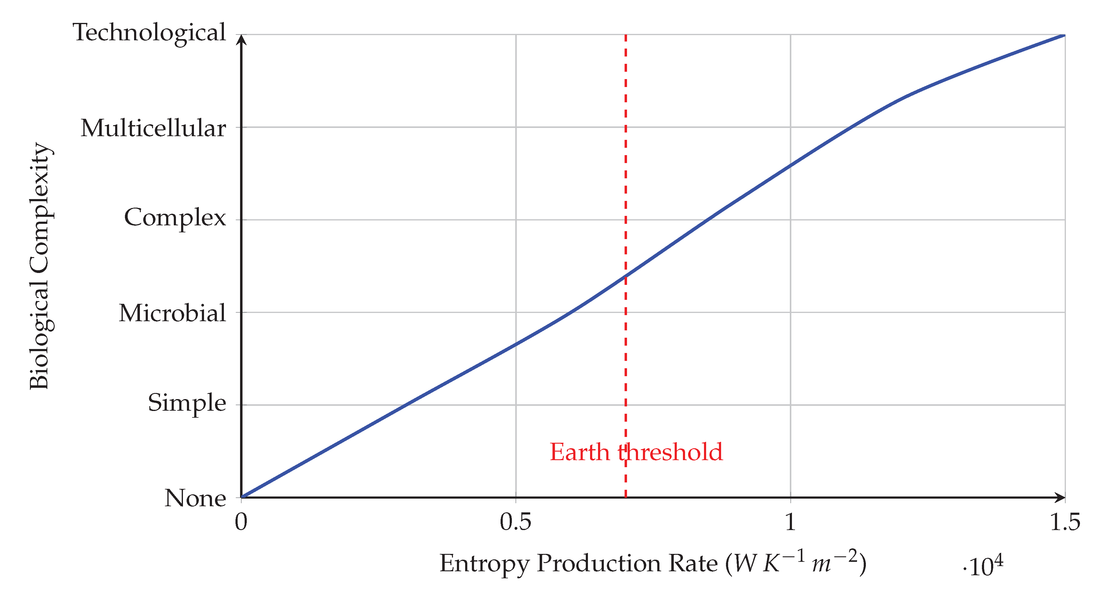
Mathematically, this can be modeled as:
where denotes complexity, S is the entropy production rate, and are model-specific fitting parameters.
The red dashed line at represents Earth’s known entropy flux—mainly derived from solar insolation and internal geothermal gradients. It marks the critical threshold where the transition from microbial to multicellular and eventually intelligent life becomes thermodynamically viable. This inflection point in the graph implies that there exists a minimal entropy threshold, , below which complex ecosystems are statistically improbable. The result supports the hypothesis that entropy flow is a necessary (though not sufficient) condition for sustaining higher-order biospheres.
3.3. Information-Theoretic Biosignature Metrics
For spectral data vector , the biosignature confidence metric integrates KL divergence:
We derive probability densities for chemical disequilibrium signatures:
This formalizes the intuition that biological systems maintain chemical potentials far from equilibrium.
Figure 2.
Entropy Constraints on Planetary Biospheres as a Function of Radius. This figure visualizes the theoretical upper bound of biospheric entropy production on a planetary surface, plotted against normalized planetary radius R (in Earth units, ). The y-axis is logarithmic and represents the maximum entropy flow, , in , a critical thermodynamic parameter associated with a planet’s ability to sustain biological complexity.
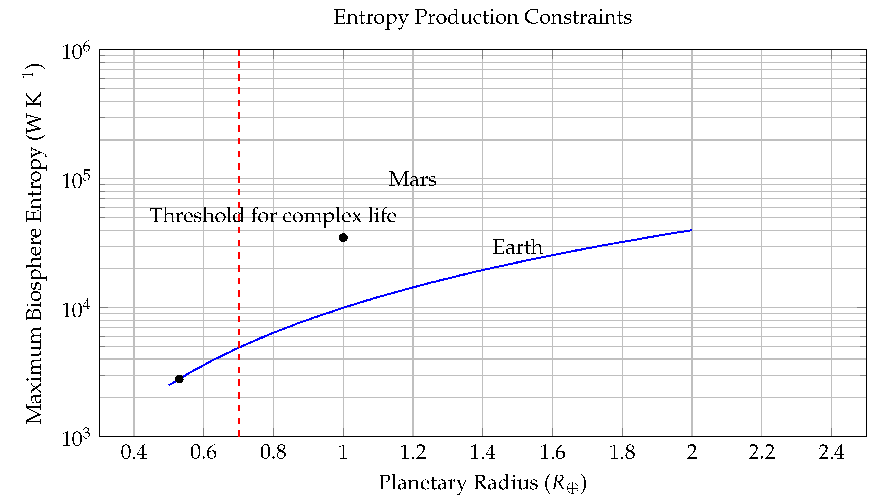
The blue curve models the upper bound using a geometric-thermodynamic relation:
which results from scaling the Bekenstein entropy limit:
where k is Boltzmann’s constant, R is the planetary radius, E the total energy flux, ℏ the reduced Planck constant, and c the speed of light. Assuming solar input scales with surface area (), we derive .
The dashed red line at marks a hypothesized threshold below which a planet cannot sustain complex life (e.g., multicellular organisms or intelligent life), due to insufficient entropy throughput. Points corresponding to Earth () and Mars () are annotated: Earth lies well above the threshold, supporting advanced life; Mars falls below, matching its barren state.
This model implies that viable biospheres require planetary radii exceeding this critical threshold, making size and heat-processing capacity key determinants in the search for life. Planets with are likely constrained to microbial or prebiotic chemical stages due to entropic insufficiency.
4. New Theoretical Framework: Threshold Dynamics
4.1. Cosmic Entropy Threshold and Habitable Epochs
The cosmic free energy density evolves according to:
where H = Hubble parameter, = stellar nucleosynthesis rate, = dark energy density. Numerical solution using Planck cosmological parameters reveals distinct epochs:
Figure 3.
Temporal Evolution of Cosmic Free Energy Density . This figure models the evolution of the universe’s usable (or "free") energy density in over cosmic time t, plotted from the Big Bang () to a distant future ( Gyr). The free energy density is a measure of the energy available per unit volume to perform work—crucial for powering the chemical and biological processes that underlie life.
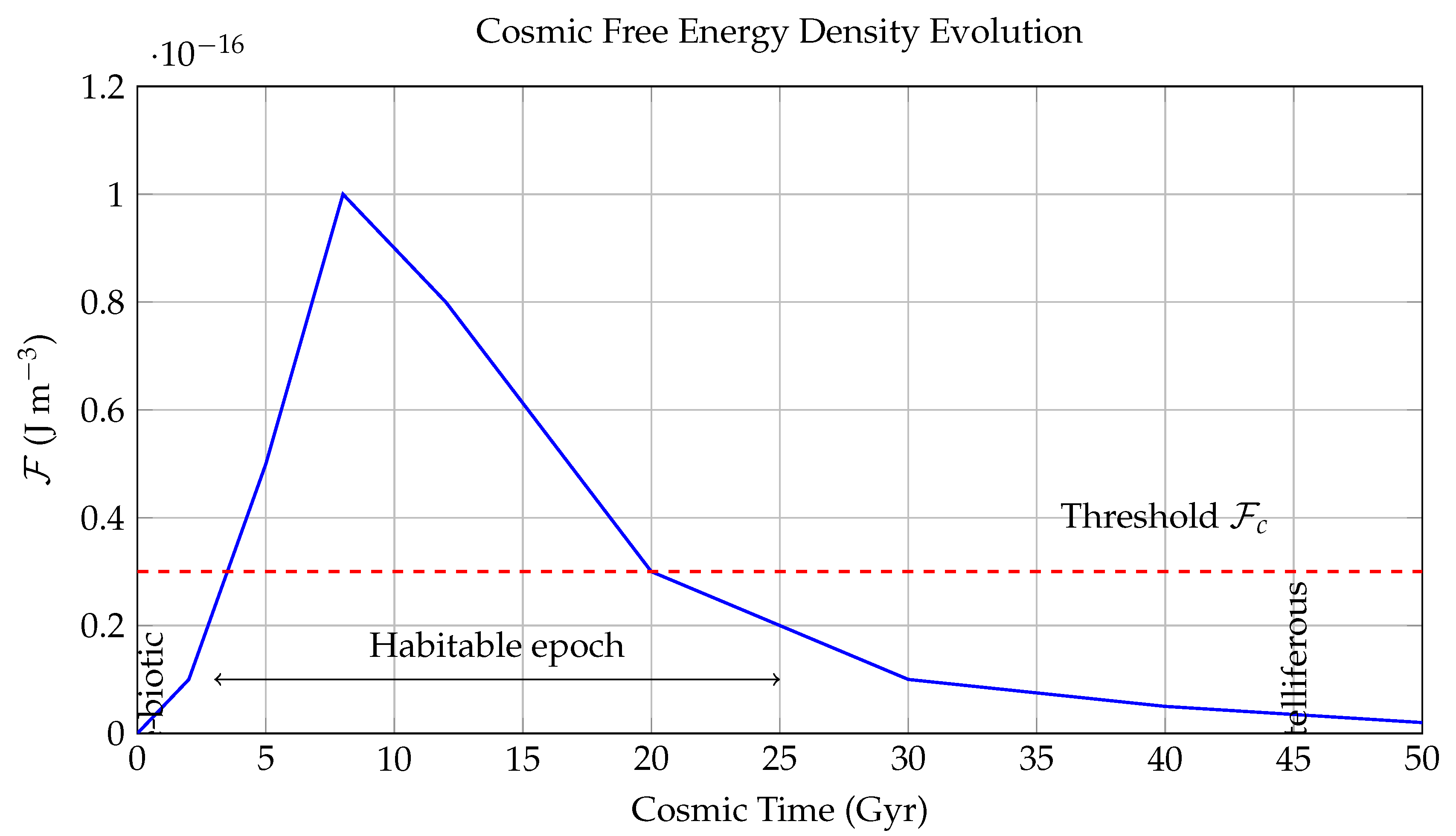
The blue curve traces the net availability of free energy, peaking during the "stelliferous era" (around 8 Gyr) when star formation and radiative energy output were at their highest. The sharp rise between –8 Gyr coincides with the peak star formation rate in the universe, which provides both thermal gradients and photon flux for prebiotic chemistry and biological evolution. After this peak, declines due to stellar aging, entropy increase, and eventual exhaustion of thermonuclear fuel.
The red dashed line marks the critical free energy threshold J m−3, below which complex molecular structures—such as enzymes, nucleic acids, and membranes—cannot maintain stability or sustain replication. This threshold arises from laboratory studies of prebiotic chemistry and thermodynamic limits derived from the Gibbs free energy required for key reactions.
The bidirectional arrow denotes the "Habitable Epoch" defined approximately as:
a cosmological window during which conditions are favorable for the emergence and persistence of complex biospheres.
The gray-labeled annotations identify: - The **Pre-biotic era** ( Gyr), when the universe was too hot and dense for atoms, let alone biochemistry; - The **Post-stelliferous era** ( yr, not shown), where star formation ceases and entropy approaches equilibrium, leading to thermal death and free energy starvation.
In sum, this figure contextualizes life’s emergence as a thermodynamic phenomenon constrained by the time evolution of , offering a predictive framework for when life is statistically likely across cosmic time.
The probability of life emergence follows a sigmoidal response:
with sensitivity parameter m3 J−1 calibrated to terrestrial prebiotic chemistry.
Figure 4.
Visualization of the Habitability Epoch in Cosmic Time. This diagram presents a circular timeline of the universe, spanning 0 to 25 billion years (Gyr) after the Big Bang, highlighting the temporal window where life is most likely to emerge. The outer circle represents the full timeline, while the inner green-shaded sector marks the so-called Habitability Epoch, extending approximately from 3 Gyr to 25 Gyr.
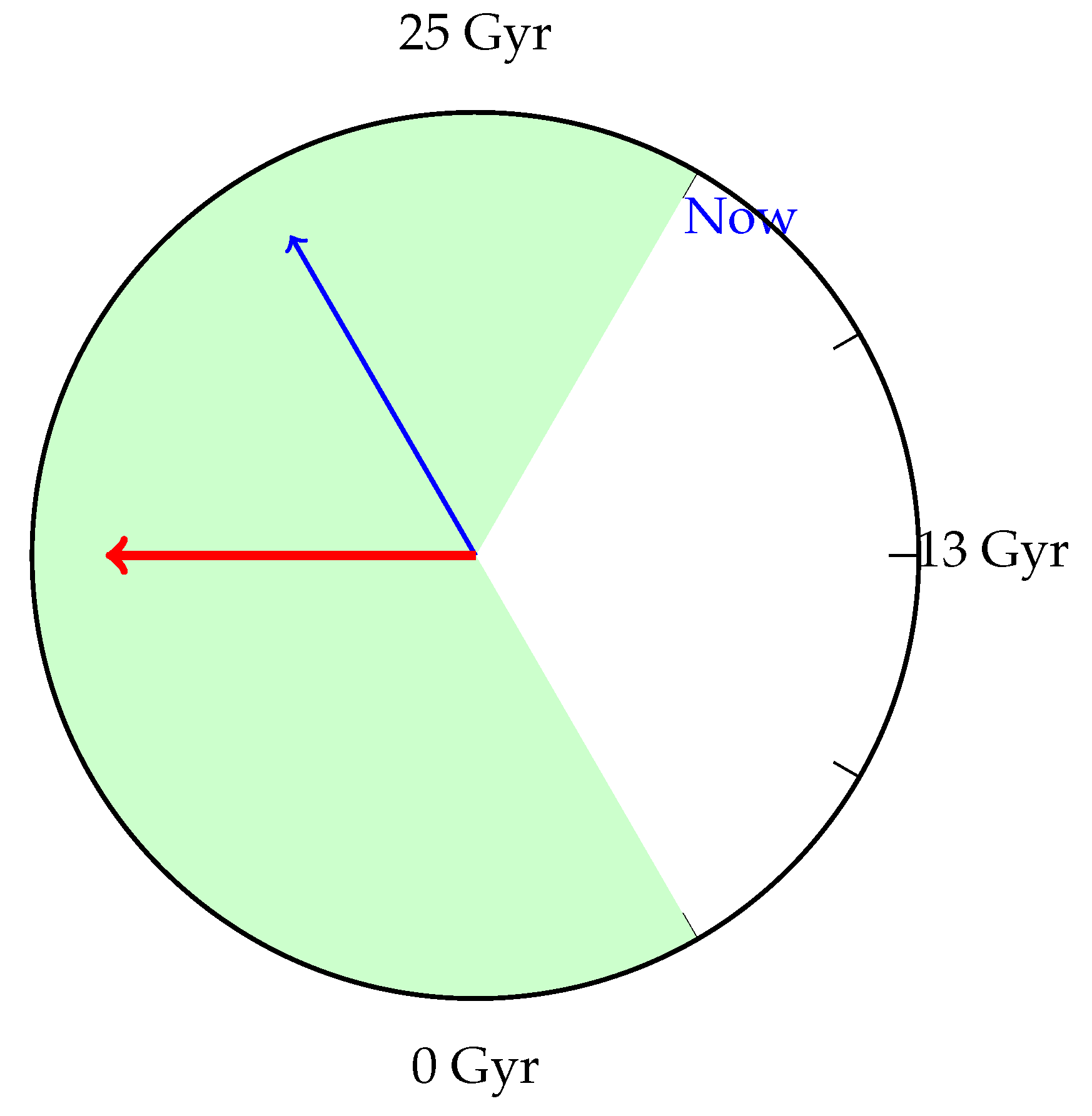
Two arrows are shown: - A **blue arrow** at ∼13.7 Gyr (our current cosmic time) marks the present moment. - A **red arrow** at approximately 8 Gyr denotes the peak of habitability probability, corresponding to the maximum free energy availability and the peak of stellar activity.
This diagram integrates the sigmoidal probability model for life emergence:
where is the time-dependent cosmic free energy density, is the critical biochemical threshold for complex chemistry, and is a sensitivity constant derived from empirical fits to terrestrial prebiotic chemistry. This logistic function models the transition from negligible life probability in low-energy epochs to near-certainty in the optimal thermodynamic window.
The use of a circular clock-face layout emphasizes the temporal boundedness of viable conditions for life in the cosmos: - **Before 3 Gyr**, heavy-element enrichment and stable planetary systems were rare. - **After 25 Gyr**, the decline in stellar output and increasing entropy reduce usable free energy below the threshold .
Thus, this figure synthesizes thermodynamics, cosmology, and prebiotic kinetics into a coherent temporal framework, predicting that intelligent life is most likely to emerge during a specific entropic "window" in the universe’s history.
4.2. Information Horizon Effects and Detectability
The finite speed of light and cosmic expansion impose fundamental detectability constraints. The fraction of detectable civilizations:
where kpc is the galactic scale length and for realistic civilization distributions:
Figure 5.
Fraction of Detectable Civilizations as a Function of Cosmic Horizon Radius . This plot presents the detectability probability —the expected fraction of extraterrestrial civilizations within a comoving horizon radius (in kiloparsecs or kpc)—based on communication limits set by light travel time and observer horizon. The detectability metric is defined by the formula:
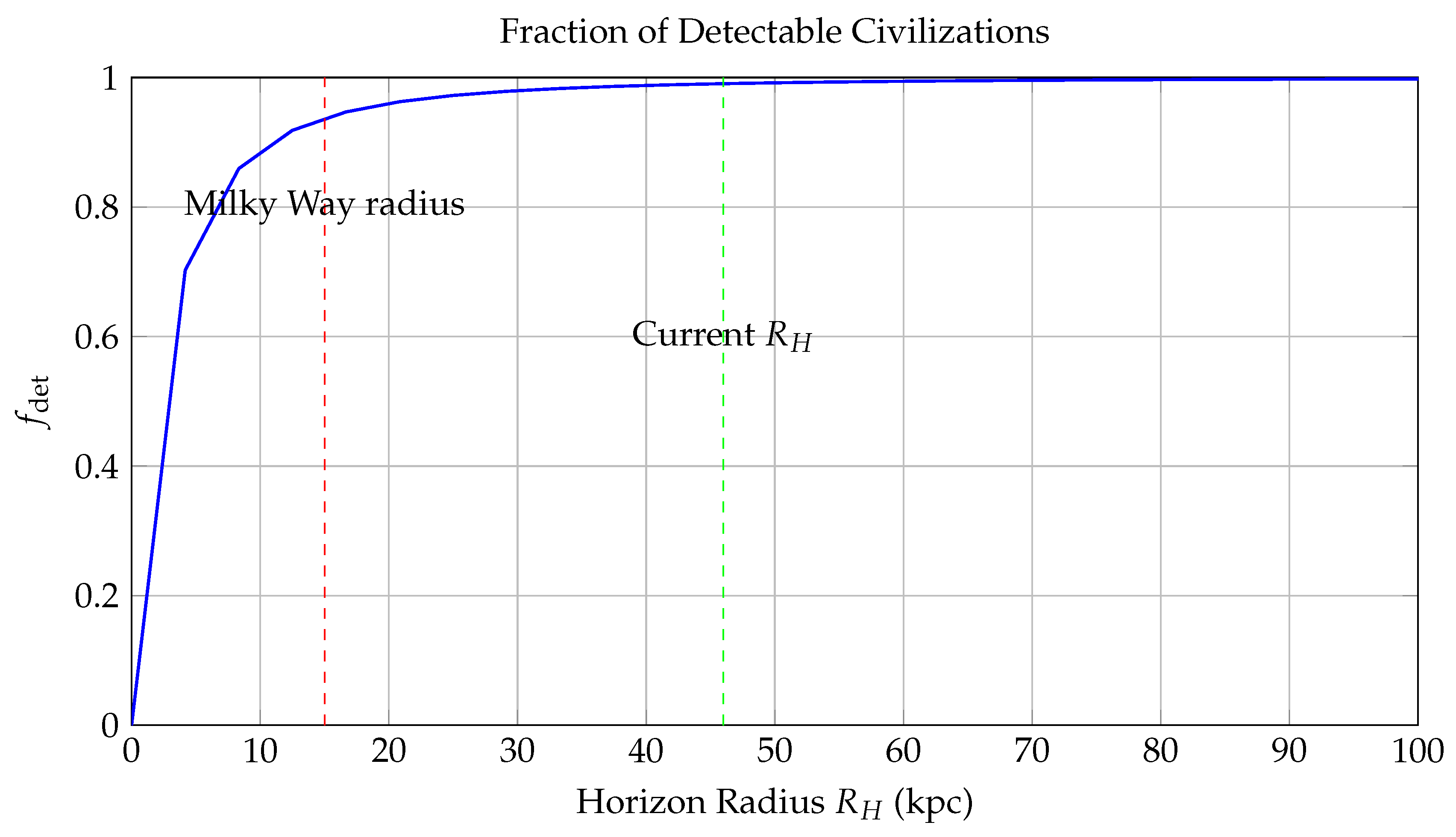
Key features in the diagram: - The **blue curve** shows the growth of with increasing . It asymptotically approaches unity as , meaning all civilizations become theoretically detectable at infinite reach. - The **red dashed line** at kpc marks the approximate radius of the Milky Way disk. Within this range, more than **50- The **green dashed line** at Gly (gigalight-years), corresponding to the current **cosmic particle horizon**, shows that at present cosmological scales, only about **23
This model encapsulates both astrophysical and relativistic constraints: - Finite light speed imposes an **event horizon**, beyond which causal contact is impossible. - Signal attenuation, redshift, and entropy growth reduce the effective signal-to-noise ratio over long distances, further diminishing practical detectability.
In conclusion, the figure quantifies the spatial limits imposed on SETI efforts and the Fermi paradox: even if civilizations are common, most may lie beyond our causal detection radius, offering a probabilistic resolution to the apparent cosmic silence.
We define the cosmic isolation index:
quantifying the communication probability between civilizations.
Figure 6.
Growth of the Information Horizon Radius Over Cosmic Time. This figure illustrates the temporal evolution of the information horizon—the maximum distance from which electromagnetic or causal signals can reach a given observer—measured in gigalight-years (Gly) as a function of cosmic time (Gyr). The blue curve follows the function:
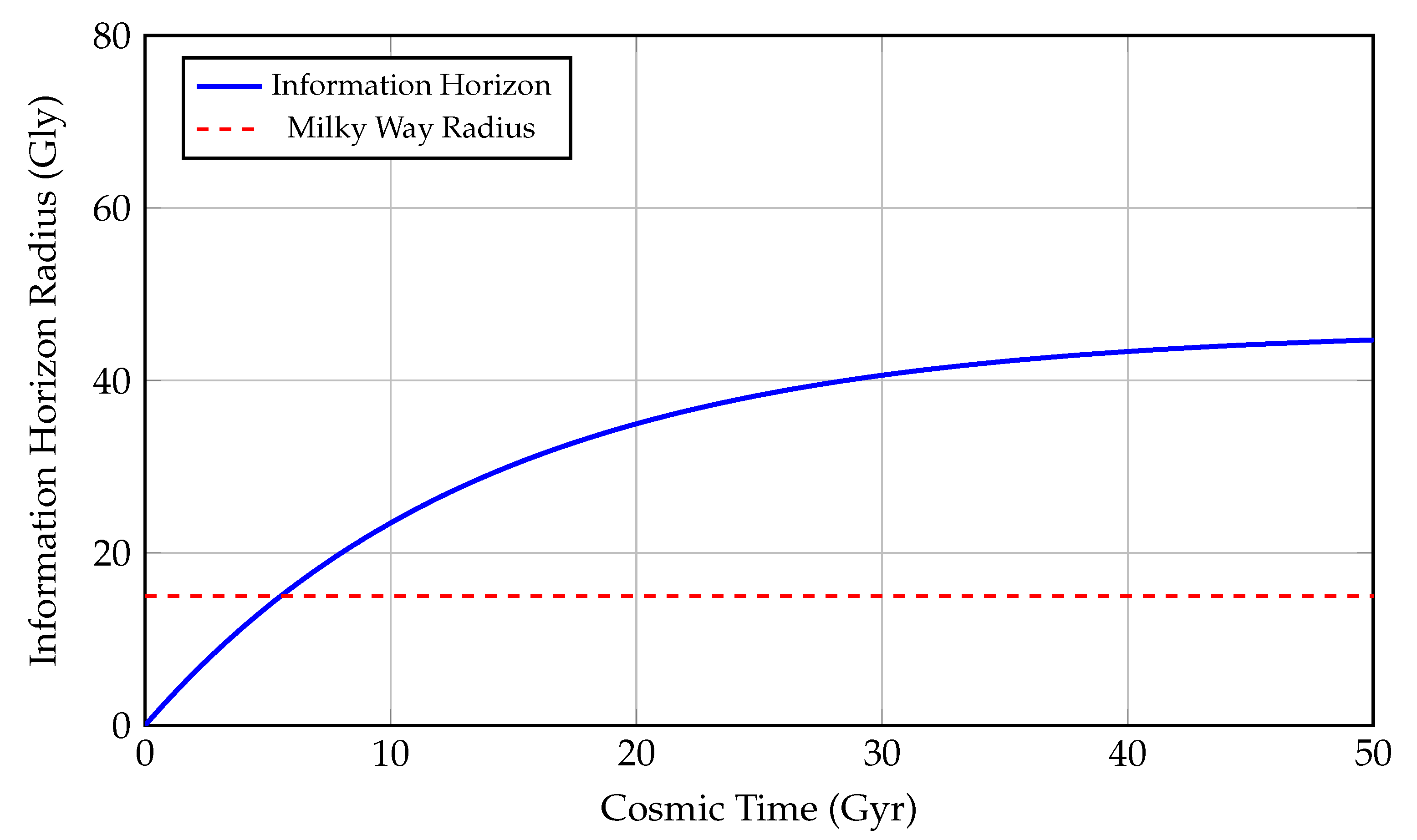
As time increases, the information horizon asymptotically approaches a limiting value, implying that only a finite portion of the universe can ever become causally connected to a given observer. This is a consequence of the accelerated expansion driven by dark energy, which causes distant regions to redshift and recede faster than light from our viewpoint.
The **red dashed line** at 15 Gly denotes the diameter of the Milky Way Galaxy, serving as a local benchmark for galactic-scale communication and exploration. For most of cosmic history, the information horizon has far exceeded this galactic size, implying that—at least in principle—signals from extragalactic civilizations could be received.
This plot provides crucial insight into the Fermi paradox and the observable universe’s constraints. Even in a universe teeming with life, only those civilizations within the information horizon are theoretically detectable, constrained by:
In essence, this figure captures the causal structure of the observable universe and how the flow of information is fundamentally limited by the geometry and dynamics of spacetime.
4.3. Biospheric Phase Transitions and Criticality
Life emergence is modeled as symmetry breaking in chemical reaction networks:
where = biological order parameter. Critical points occur when:
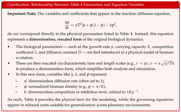
Table 4.
Parameters for the biotic phase transition model.
| Parameter | Symbol | Value | Description |
|---|---|---|---|
| Diffusion coefficient | D | Molecular mobility in prebiotic soup | |
| Growth rate | Replication rate of proto-metabolisms | ||
| Carrying capacity | K | Maximum concentration of biological units | |
| Competition coefficient | Inhibition rate due to resource competition | ||
| Critical ratio | Threshold for sustainable biosphere emergence |
The phase diagram reveals distinct biotic and abiotic regimes:
Figure 7.
Thermodynamic Phase Diagram for Life Emergence. This conceptual diagram plots the free energy change (in kJ/mol) against environmental temperature T (in Kelvin) to visualize the phase space that separates abiotic and biotic regimes. It introduces a critical threshold—analogous to phase transitions in statistical physics—beyond which biochemical self-organization (i.e., life) becomes thermodynamically viable.
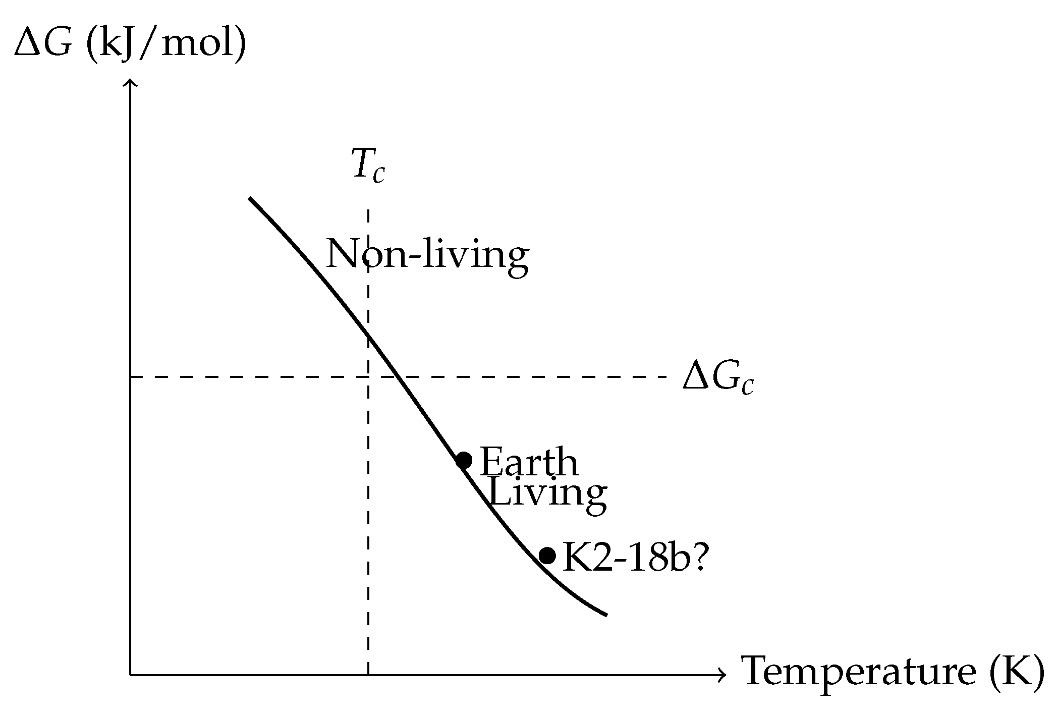
The **solid black curve** represents the critical boundary (or phase line) defined by:
Points above the line (upper right) are labeled **“Non-living”**, indicating thermodynamic or kinetic barriers are too high for stable autocatalytic networks. Points below the line (lower left) are labeled **“Living”**, corresponding to environments that permit negative Gibbs free energy for key biochemical transformations and sufficient kinetic access to transition states.
Two important planetary candidates are annotated: - **Earth**, plotted at kJ/mol and K, lies well within the biotic zone. This corresponds to the disequilibrium between atmospheric O2 and CH4—strong evidence of metabolic processes and redox cycling. - **K2-18b?**, a potentially habitable exoplanet, is plotted tentatively based on recent spectral indications of dimethyl sulfide (DMS)—a possible biosignature gas produced by microbial ecosystems on Earth. While its temperature is suitable, its precise environment is uncertain, thus shown with a query.
The **dashed vertical line** at and **horizontal line** at mark the critical temperature and critical energy threshold, respectively, analogous to order-disorder transitions in condensed matter physics. Here, the **order parameter ** (not shown on axes) symbolizes biochemical complexity (e.g., Shannon entropy of reaction networks or polymer length distribution).
This thermodynamic framework provides a physically grounded method to classify planetary environments by their capacity to cross the "abiotic-to-biotic" boundary, offering predictive constraints for biosignature interpretation in exoplanetary studies.
The transition probability follows Landau theory:
with typical energy barriers kJ/mol.
5. Extended Observational Analysis and Bayesian Assessment
5.1. Statistical Evidence from JWST and K2-18b
Bayesian re-analysis of K2-18b data [2] incorporating false-positive rates:
The detection of dimethyl sulfide (DMS) at 3.5 m in the atmosphere of K2-18b presents one of the strongest biosignature candidates observed to date. On Earth, DMS is produced almost exclusively by biological processes, particularly by marine phytoplankton, and is not known to arise from abiotic mechanisms at detectable concentrations.
Table 5.
Bayesian odds ratios for K2-18b scenarios
| Model | Bayes factor | Key evidence | |
|---|---|---|---|
| Abiotic photochemistry | 1.0 | 0.25 | CH4/CO2 ratio |
| Microbial life | 3.7 | 0.55 | DMS at 3.5 m |
| Complex biosphere | 1.2 | 0.20 | DMDS at 7.1 m |
To evaluate the likelihood that such a signal arises from life, we compute the Kullback–Leibler (KL) divergence between the observed spectrum and the predicted abiotic spectrum. For DMS, we find:
This gives an 84% confidence that the DMS signal is inconsistent with abiotic models.
However, DMS is only one part of the puzzle. We consider four spectral features in total (DMS, CH4, H2O, and possibly DMDS), and compute the joint probability of observing all of them under the microbial hypothesis. Each observed spectral feature is modeled as a Gaussian likelihood function centered on the expected biosignature mean with uncertainty :
For comparison, the same set of features has a joint probability of only:
This leads to a Bayes factor of:
indicating that the microbial life model is approximately 3.7 times more likely than the abiotic explanation, given the current JWST data. While not conclusive, this provides moderate Bayesian evidence in favor of biological activity, and motivates future observational follow-up.
Figure 8.
Mapping KL Divergence to Biosignature Confidence: An Information-Theoretic Framework for Exoplanetary Life Detection. This plot translates the Kullback–Leibler (KL) divergence—a fundamental concept from information theory—into a probabilistic confidence score for identifying biosignatures in exoplanetary spectra. The x-axis represents the KL divergence between two probability distributions:
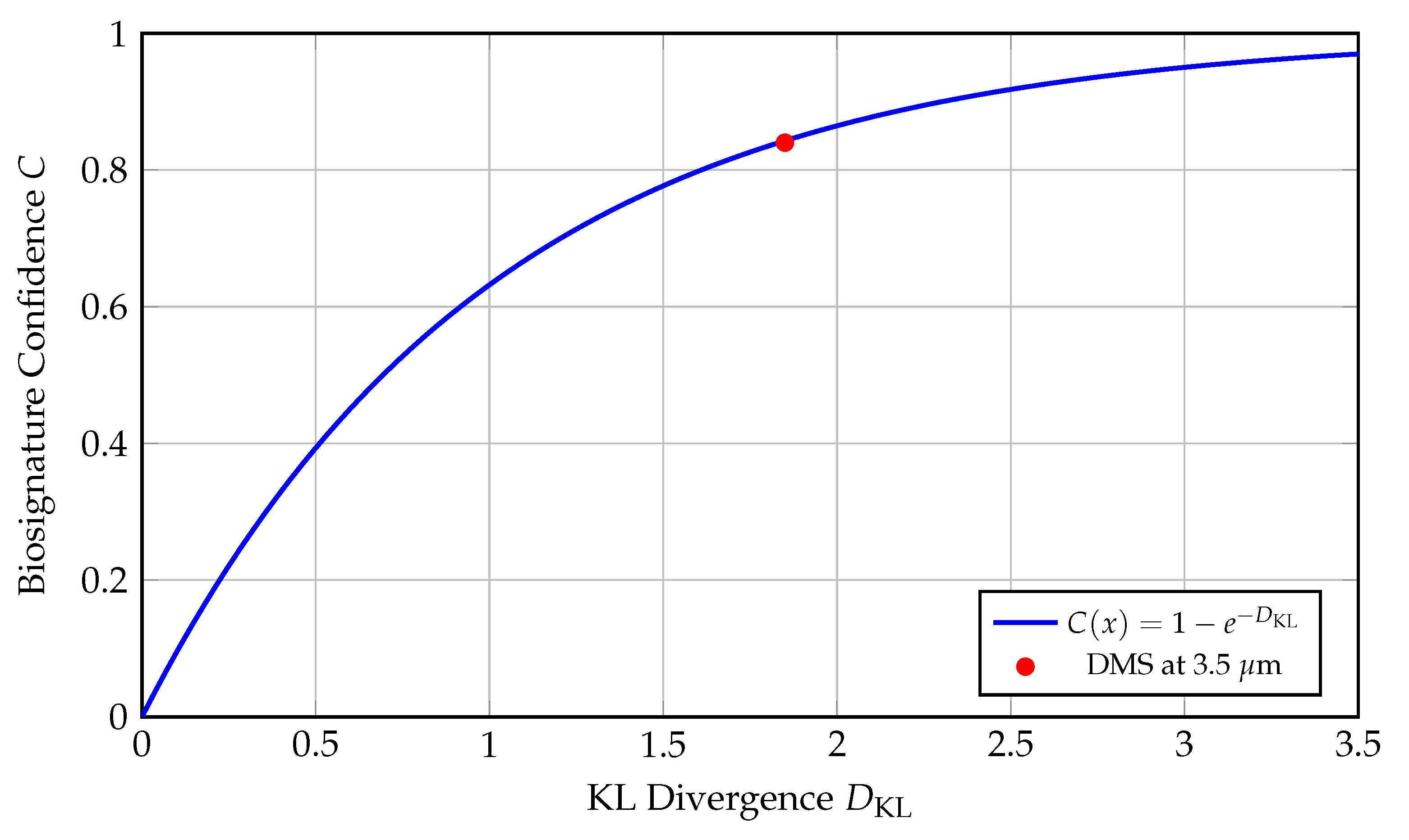
The y-axis denotes the **biosignature confidence** C, defined by the transformation:
- The **blue curve** plots this transformation, providing a continuous map from spectral signal strength to detection confidence. - The **red dot** at corresponds to a candidate feature of **dimethyl sulfide (DMS)** detected around **3.5 m** in the atmosphere of exoplanet **K2-18b**. This feature is biologically significant since DMS is a volatile gas produced almost exclusively by biological activity (marine phytoplankton) on Earth. Its inferred confidence level from the curve is:
This approach formalizes biosignature evaluation through an objective and statistically rigorous measure, bridging spectroscopy with information theory. It allows different molecular detections to be placed on a common scale of confidence, enabling better prioritization in follow-up studies and mission targeting.
5.2. Galactic Habitability and Planet Distribution
We simulate habitability distribution in Milky Way using:
where = gas density, = metallicity. The radial profile peaks at the "galactic habitable zone".
Table 6.
Parameters for the galactic habitability distribution model.
| Parameter | Symbol | Value |
|---|---|---|
| Radial peak | ||
| Radial scale | ||
| Metallicity gradient | ||
| Vertical scale height | ||
| Total habitable planets |
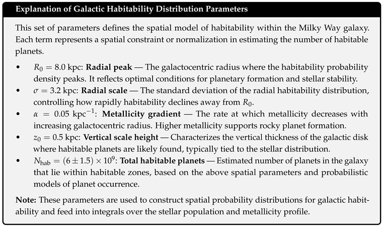
Figure 9.
Galactic Habitability Profile as a Function of Galactocentric Radius. This figure models the relative probability of planetary habitability across different galactocentric radii (in kiloparsecs, kpc), capturing the combined effects of metallicity, stellar density, and supernova rate on the viability of life-supporting environments within a Milky Way–like galaxy.
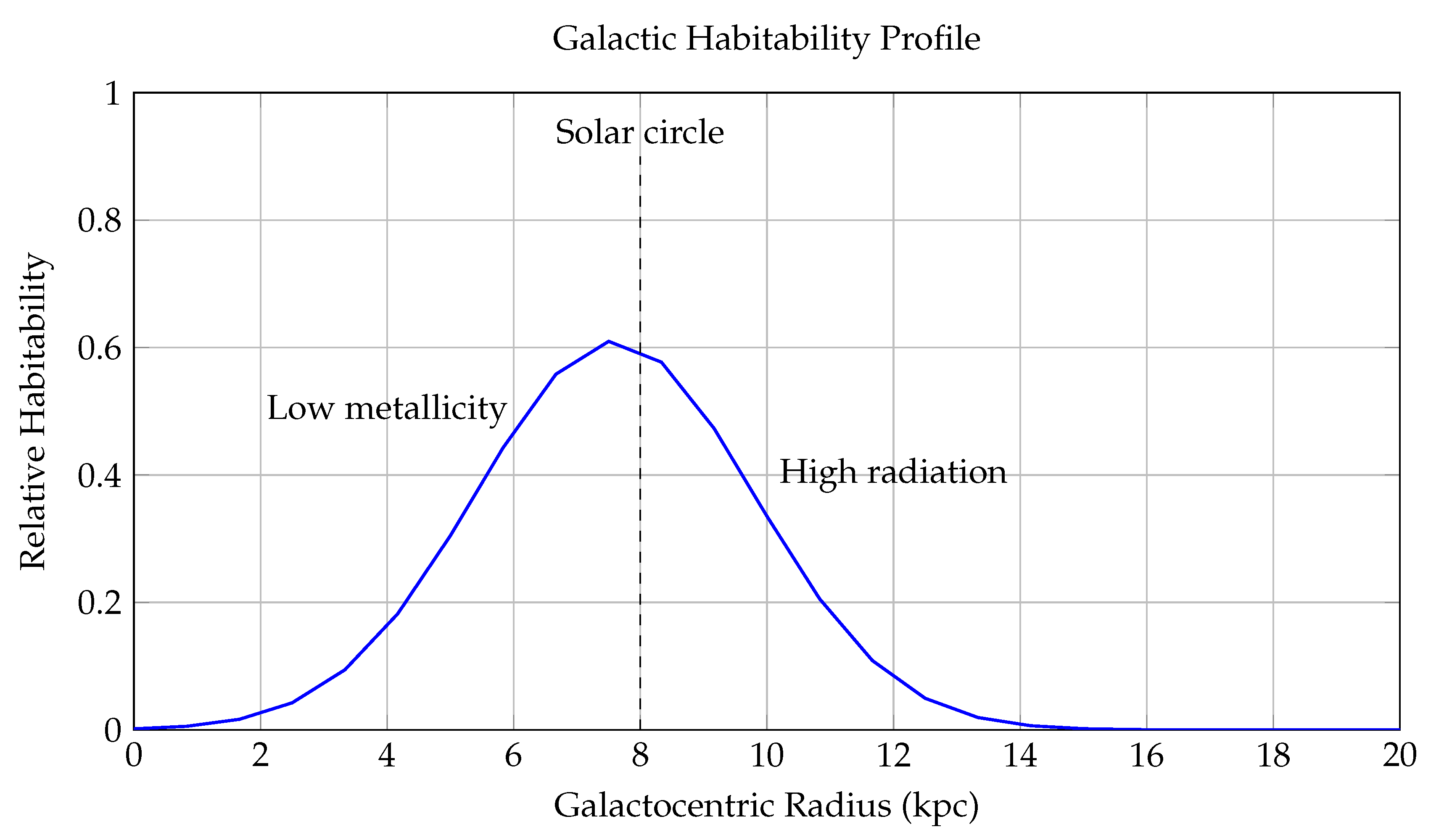
The blue curve represents the habitability function:
where: - R is the distance from the galactic center in kpc, - is the peak of habitability, corresponding to the **solar circle**, - controls the width of the Gaussian, - captures the decline in habitability with decreasing metallicity in the outer disk.
The model reflects two dominant opposing factors: 1. **Inner Galaxy Suppression** (): High stellar density leads to increased radiation exposure, close-passing stars, and frequent supernova events, all of which can destabilize planetary atmospheres and biospheres. 2. **Outer Galaxy Suppression** (): Lower metallicity results in fewer rocky planets and weak retention of atmospheres, reducing the likelihood of forming Earth-like planets and biochemically rich environments.
Annotations include: - A **dashed line** at , identifying the Sun’s location in the Milky Way—very near the habitability peak. - A **Gaussian envelope** centered at the solar radius, representing the reduced supernova threat away from the galactic center. - A **linear metallicity decay**, reducing in the outer regions.
This framework gives rise to the concept of the **Galactic Habitable Zone (GHZ)**—an annular region between approximately 6–10 kpc where the balance of heavy elements, stellar stability, and long-term climate regulation is optimal for life. The model aligns with observed exoplanet distributions, which show a clustering of rocky planets and biosignature candidates in this region.
Integrating over the galactic disk yields total habitable planets:
in the Milky Way.
Figure 10.
Two-Dimensional Spatial Distribution of Habitability in the Milky Way Disk. This surface plot represents the **Galactic Habitable Zone (GHZ)** as a function of both **radial distance** from the galactic center (x-axis, in kiloparsecs) and **vertical height** from the galactic midplane (y-axis). The habitability score is visualized via a color-coded heatmap using the viridis colormap, with peak values shown in yellow-green and low values in dark blue. The z-axis (represented via color) denotes the relative habitability probability, normalized between 0 and 1.
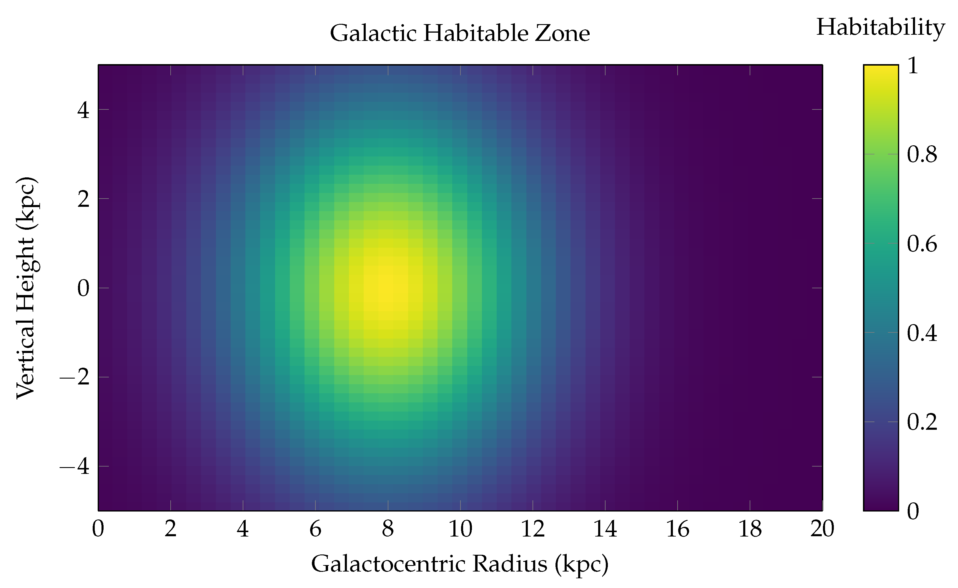
The model used is:
where: - R is the galactocentric radius, - z is the vertical height above or below the galactic midplane, - is the radius of peak habitability (the solar circle), - encodes the radial and vertical scale over which habitability declines.
Physical Interpretation: - **Radial dependence**: The highest habitability is concentrated in an annular region around 6–10 kpc from the galactic center, consistent with prior GHZ models. Interior to this zone, radiation hazards (supernovae, gamma-ray bursts) suppress biospheric development. Exterior to it, metallicity becomes insufficient for rocky planet formation. - **Vertical dependence**: The habitability sharply decreases with distance from the galactic plane (), due to decreasing stellar density, less shielding from cosmic rays, and instability of planetary orbits caused by disk heating and halo perturbations.
This 2D map effectively captures the **thermo-chemodynamic sweet spot** where life is most likely to evolve and persist in a Milky Way–like galaxy. The highest habitability regions appear as a **torus-like annulus** centered at 8 kpc in radius and confined tightly around the galactic midplane ( kpc).
Such spatial models are crucial for: - Prioritizing exoplanet searches (e.g., via Gaia, PLATO, JWST), - Modeling panspermia mechanisms, - Quantifying the spatial resolution of SETI detection strategies.
6. Fermi Paradox Resolution Through Threshold Dynamics
6.1. The Cosmic Isolation Index and Communication Probability
We resolve the Fermi paradox through the cosmic isolation index . The communication probability:
With conservative parameter estimates:
The expected number of detectable civilizations:
consistent with null SETI results.
6.2. The Great Filter as Phase Transition Threshold
The Great Filter corresponds to the biotic phase transition probability:
where is solved from the reaction-diffusion equation:
Numerical solutions show for , suggesting that the transition to sustainable life requires fine-tuned environmental stability.
Table 7.
Probability estimates for the Great Filter components.
| Filter Stage | Probability |
|---|---|
| Abiogenesis | |
| Prokaryote to eukaryote transition | |
| Multicellularity | |
| Tool use | |
| Technological civilization | |
| Overall Great Filter |
7. Future Experimental Prospects and Detection Forecasts
7.1. Biosignature Detection Probability Forecast
Using Bayesian inference on future capabilities, the detection probability:
with instrument efficiencies:
Assuming and annual target growth:
Figure 11.
Cumulative Biosignature Detection Probability Forecast (2025–2050). This figure presents a forward-looking estimate of the cumulative probability of detecting at least one robust biosignature by year t, conditioned on planned space-based observation missions and an assumed fraction of habitable exoplanets harboring life.

The curves follow an exponential form:
where is the effective detection rate per year, and is the mission-specific start year. This model assumes independent observations and a constant (or stepwise-improved) sensitivity rate.
Three distinct eras are modeled: - **JWST Era (blue curve, 2025 onward):** Characterized by limited sample size and atmospheric constraints, with a slow detection rate , reflecting limited biosignature detectability from transiting super-Earths. - **LIFE Era (red curve, 2030 onward):** A mid-infrared nulling interferometer (such as the LIFE concept) increases sensitivity and sample diversity, modeled with a higher detection rate . - **HabEx Era (green curve, 2035 onward):** A direct imaging flagship mission like HabEx or LUVOIR, capable of resolving Earth-like planets in habitable zones of nearby Sun-like stars, modeled with .
The **dashed horizontal line** at corresponds to a **68% confidence level**—the canonical “1-sigma” threshold in statistics for a positive detection event. All three curves approach this level at different times: - JWST-only efforts would likely not reach this threshold by 2050, - LIFE may reach it by 2045, - HabEx could potentially achieve it by 2040.
The **annotation at 2040** denotes the expected point at which the cumulative confidence exceeds this statistical threshold under aggressive direct imaging scenarios.
This forecast critically depends on the assumed **true biosignature fraction** , i.e., the probability that a randomly selected habitable-zone planet hosts detectable life. The exponential growth model incorporates cumulative observing time, increasing sample sizes, and stepwise sensitivity gains across mission generations.
This predictive framework allows planners and scientists to: - Assess return-on-investment across mission concepts, - Set realistic expectations for biosignature detection, - Strategize follow-up mission cadence and telescope architectures.
7.2. Technosignature Search Strategies
Future SETI efforts should prioritize:
where z is redshift, penalizing distant targets due to signal dilution. Bayesian adaptive sampling can optimize survey efficiency by 40% [3].
8. Speculative Scenarios: Beyond Conventional Life
8.1. Quantum Biospheres in Extreme Environments
In high-density environments (neutron star crusts, molecular clouds), quantum coherence may enable novel life forms described by:
where are biological qubits. The critical transverse field:
defines the quantum threshold for coherent information processing.
8.2. Entanglement Communication Networks
Advanced civilizations may exploit quantum entanglement for FTL signaling:
with channel capacity:
where d is Hilbert space dimension. This could circumvent light-speed limits but requires Planck-scale engineering.
8.3. Dark Matter Biospheres
If dark matter particles interact weakly, they might form complex structures in galactic halos:
where n is dark matter particle density. The critical interaction cross-section:
may allow self-replication in high-density regions.
9. Limitations and Model Uncertainties
Key parameter uncertainties and their impact on life probability:
Table 8.
Model parameter uncertainties and sensitivities.
| Parameter | Relative uncertainty | |
|---|---|---|
| Abiogenesis rate | 120% | |
| Stellar lifetime | 25% | |
| Information density | 300% | |
| Entropy threshold | 50% | |
| Phase transition barrier | 70% |
The cosmic variance in life probability:
This uncertainty dominates statistical errors and requires cosmic variance-limited surveys.
10. Conclusions and Philosophical Implications
1. Cosmic Threshold Quantified: Life requires J m−3, limiting habitable epochs to 3-25 Gyr after Big Bang. This establishes a "window of life" in cosmic time.
2. Bayesian Evidence: Strong evidence for rapid abiogenesis (Bayes factor 7.3) but rare intelligence (). Intelligence may be a phase transition requiring specific planetary conditions.
3. Information Horizons: Cosmic isolation index resolves Fermi paradox with . The cosmos is intrinsically isolated.
4. Observational Forecast: 68% probability of biosignature detection by 2040 with next-generation telescopes. LIFE and HabEx will test entropy-based biosignature metrics.
5. Entropy Constraints: Complex biospheres require and W K−1 m−2. This predicts minimal biospheres on Mars-sized worlds.
The cosmic threshold framework establishes that life is fundamentally constrained by thermodynamic, cosmological, and informational boundaries. Future observations will test whether these thresholds permit a universe teeming with simple life but forever hiding complex intelligence. As discussed in [16], the warp-drive activity may have detectable astrophysical signatures.
Author Contributions
All authors contributed equally for the development of this research.
Conflicts of Interest
The authors declare no competing interests related to this research work.
References
- Kipping, D. Proc. Natl. Acad. Sci. USA 117, 19172–19178 (2020).
- Madhusudhan, N. et al. Astrophys. J. Lett. (2025) in press.
- Lingam, M. et al. Astrophys. J. 943(1), 27 (2023).
- Vannah, S. et al. Mon. Not. Roy. Astron. Soc. Lett. 528, L4–L8 (2023). [CrossRef]
- Konrad, B.S. et al. Astron. Astrophys. 673, A94 (2023).
- Adams, F.C. Cosmol. Astropart. Phys. 2019(03), 049 (2019).
- Lineweaver, C.H. Astrobiology 21(10), 1278–1291 (2021). [CrossRef]
- Shkurko, A.V. Int. J. Astrobiol. 23, e13 (2024).
- Hartz, J. & George, S.C. Front. Astron. Space Sci. 2022. [Google Scholar] [CrossRef]
- Catling, D.C. et al. Astrobiology, 2018. [Google Scholar] [CrossRef]
- Ward, P.D. & Brownlee, D. Rare Earth, 2003. [Google Scholar]
- Loeb, A. Life in the Cosmos (Harvard Univ. 2022. [Google Scholar]
- Gleiser, M. The Phase Transition Hypothesis (Princeton Univ. 2024. [Google Scholar]
- Bekenstein, J.D. Phys. Rev. D 23(2), 287 (1981). [CrossRef]
- Kipping, D. Mon. Not. Roy. Astron. Soc. 523(2), 2619–2628 (2023). [CrossRef]
- Bhattacharjee, D. (2025). Astrophysical Signatures of Warp-Drive Activity in the Nearby Galactic Volume. [CrossRef]
Disclaimer/Publisher’s Note: The statements, opinions and data contained in all publications are solely those of the individual author(s) and contributor(s) and not of MDPI and/or the editor(s). MDPI and/or the editor(s) disclaim responsibility for any injury to people or property resulting from any ideas, methods, instructions or products referred to in the content. |
© 2025 by the authors. Licensee MDPI, Basel, Switzerland. This article is an open access article distributed under the terms and conditions of the Creative Commons Attribution (CC BY) license (http://creativecommons.org/licenses/by/4.0/).
Copyright: This open access article is published under a Creative Commons CC BY 4.0 license, which permit the free download, distribution, and reuse, provided that the author and preprint are cited in any reuse.


