
Submitted:
14 July 2025
Posted:
15 July 2025
You are already at the latest version
Abstract
Local scour around bridge piers is a leading cause of structural failure. Therefore, the estimation of maximal scour depth (dsm) is essential. Many studies in the last eight decades have included metadata collection and developed around 80 empirical formulas using various scour-affecting parameters of different ranges. To date, a maximum of 33 formulas have been comparatively analyzed and ranked based on their predictive accuracy. In this study, novel formulas using semi-empirical methods and gene expression programming (GEP) have been developed alongside an artificial neural network (ANN) model to accurately estimate dsm using 768 observed metadata points collected from 40 literatures, along with eight newly conducted experimental data in the laboratory. These new formulas/model are systematically compared with 74 empirical literature formulas for their predictive capability. The influential parameters for predicting dsm, in this study, are flow intensity, flow shallowness, sediment gradation, sediment coarseness, time, constriction ratio, and Froude number. Performances of the formulas/models are compared using different statistical metrics such as the coefficient of determination, Nash-Sutcliffe efficiency, mean bias error, and root-mean-squared error. The Gauss-Newton method is employed to solve the nonlinear least-squares problem to develop the semi-empirical formula that outperforms the literature formulas, except the formula from GEP, in terms of statistical performance metrics. However, the feed-forward ANN was found to be the best model among all, providing approximately 15-18 % greater accuracy with minimal errors and narrower uncertainty bands. Using user-friendly tools and a strong semi-empirical model, which requires no coding skills, can assist designers and engineers in making accurate predictions in practical bridge design and safety planning.
Keywords:
maximum scour
; gene expression programming
; artificial neural network
; Gauss-Newton algorithm
; Levenberg-Marquardt algorithm
1. Introduction
Scour, a natural occurrence, results from the erosive force of flowing streams on erodible beds, risking the integrity of the bridge structure [1,2]. The study of bridge scour has been divided into two major fields scientific inquiry seeks to understand the scour process academically, while engineering endeavors aim to offer practical guidance for implementation such as scour depth (ds) estimating (flume tests, empirical formula, data-driven soft computing technique) monitoring and countermeasure [3,4].
Many scour prediction formulas have been developed to predict equilibrium scour depth (dse) using flume tests [5,6,7,8,9], temporal scour variations [10,11,12,13], and maximum scour depth (dsm) incorporating the time factor [14,15]. Several distinguished researchers have contributed significantly to the design method for time-dependent local scour as well [16,17,18]. After investigations by several researchers, an understanding of dsm around circular piers has been achieved mostly for sand beds [19,20] and very few for gravel beds [21] in clearwater conditions. The data-driven approach using different ensemble machine learning models to address circular bridge piers [22,23,24,25,26,27] has been studied recently. Empirical formulas for live-bed and clearwater scour were both developed by several researchers [28,29,30,31].
Empirical formulas: Major findings and limitations of some literatures are addressed below. Lacey [32] and Inglis [33] developed regime formulas using data from irrigation canals in India. Kothyari et al. [34] commented on the Lacey–Inglis method specifically designed for non-cohesive sands with sediment mean size (D50) of 0.15-0.43 mm and gradation (σ) of 1.4-1.8, used for designing railways and road bridges in India [29]. Vijayasree and Eldho [35] found that the IRC formula underestimates ds by overlooking pier geometry. They modified IRC, with an empirical constant from experiments on various pier shapes. Gao et al. [36] developed a formula from field data, applied in Chinese infrastructure for over 20 years. This study refined the formula using hydraulic models and field data to closely align calculated results with real-world observations for scour scenarios. Ansari and Qadar [37] tested three formulas [38,39,40] for predicting ds, analyzing 100+ field observations from 12 sources and regions. Melville [41] presented a method to predict ds at piers using laboratory data. However, variations in formula structures and sensitivity of parameters can lead to significantly different predictions [42]. Federal Highway Administration guidelines recommended estimating design dsm [7]. It was developed from lab data for circular piers by Chabert and Engeldinger [43] and Colorado State University data, and widely acknowledged as a leading formula for predicting dsm. Benedict and Caldwell [44] reviewed literatures to find pier scour, compiling 569 lab and 1,858 field measurements. Sheppard et al. [45] examined 17 formulas with 441 lab and 791 field data points. They ranked the formulas statistically and compared under-prediction errors to total errors. Manes and Brocchini [46] developed a scale-independent formula for dse at a circular pier in a granular bed. Vonkeman and Basson [47] evaluated 30 empirical formulas with their 48 experiments and revealed different results, especially for non-circular piers. Coscarella et al. [48] presented new hypotheses on momentum transport and bed shear stress, questioning conventional thinking after Manes and Brocchini [46], and developed a formula for predicting dsm. Franzetti et al. [14] developed another dsm formula integrating metadata from literature. In addressing temporal ds measurements, Nandi and Das [15] compared 11 literature formulas and developed one formula to predict dst. Equilibrium methods for predicting ds face well-documented limitations, with studies noting inconsistencies in dse and te definitions, which lead to ambiguity and inaccuracies in predictions [49,50]. This lack of a universal criterion complicates experiments, field studies, and data analysis, contributing to database inconsistency and uncertainty [51,52]. The evaluation of 74 empirical prediction formulas (Section S1) illustrates the varied strengths, limitations, and drawbacks of these methods (Section S2). Many existing formulas for predicting ds used limited parameter sets based on specific experimental conditions, which may introduce some degree of inaccuracy [53]. While some formulas tend to show good agreement within the datasets they were originally derived from [54,55]. Some formulas may slightly overestimate or underestimate dsm compared to observed data, highlighting areas where predictive accuracy could be further refined [56,57]. The detailed dimensional information comparing the thorough literature review of experimental and numerical studies around isolated (Table S1) and complex piers (Table S2) is given respectively in the supplementary information. Some approaches excel under specific conditions but may be less accurate across varied datasets, suggesting that a broader parameter inclusion might enhance their applicability.
Data-driven stand-alone and hybrid ML models: The studies have used GEP techniques to predict ds around bridge piers, significantly improving prediction accuracy compared to traditional empirical models [58]. Rathod et al. [59] demonstrated that support vector machine (SVM) outperformed other artificial intelligence algorithms like ANN, adaptive neuro-fuzzy inference system (ANFIS), and gene expression programming (GEP) in predicting ds. Eini et al. [60] employed hybrid models combining particle swarm optimization and XGBoost, finding that RPSO-XGBoost provided better results for ds estimation. Kumar et al. [25] utilized ensemble methods like bagging regressor and adaboost regressor, showing enhanced performance over individual models like SVR. Shalini et al. [61] highlighted the success of the ANFIS model, outperforming other techniques, while Ahmadianfar et al. [62] improved ds predictions around pile groups using an ensemble approach. Pandey et al. [63] found that the CatBoost model outperforms extra tree regression and K-nearest neighbor in predicting ds around abutments. Choudhary et al. [64] developed ANFIS and GEP models to accurately predict ds around bridge piers under clear-water and live-bed conditions. Using key hydraulic and sediment parameters, the ANFIS model proved highly accurate (CD ≈ 0.95) across most cases, though it showed limitations when the pier was relatively narrow compared to flow depth in live-bed scenarios. Recent work by Baranwal and Das [65] and Kumar et al. [66] continued to explore the efficacy of models like M5Tree, XGBoost, and random forest, demonstrating superior predictive accuracy across different datasets. Niknam et al. [67] showed that GEP with a three-gene configuration provided the most accurate predictions for ds around oblong piers, outperforming SVM and ANN models. A detailed table summarizing the studies that employed GEP and ANN as at least one of their ML methods for isolated pier ds modeling was included as Table S3 in the supplementary information. GEP and ANN are particularly effective for predicting ds because they are relatively easy to use with available software frameworks. These models were chosen for simplicity and strong predictive abilities, making them practical without knowing advanced programming skills.
The present research, therefore, aims to formulate robust data-driven formulas using ANN, GEP, semi-empirical approach to analyze. The present study uses 40 experimental datasets, including 768 data points obtained from 67 years of literatures. The number of datasets considered is the highest compared to previous studies. Eight functional parameters are used for inter-comparison of 74 literature formulas (highest so far), including flow intensity(V/Vc), flow shallowness (H/B), sediment gradation (σ), sediment coarseness (B/D50), dimensionless time (Vt/BΔ0.5), constriction ratio (B/W), Reynolds number (R) and Froude number (F). To capture the relationship between these parameters, different nonlinear functions were used, such as two parameters sigmoid function, bragg function, power function, exponential function, etc. The Gauss-Newton method and Levenberg-Marquardt algorithm are used to optimize the objective function. New experiments are conducted to assess the prediction performance of formulas.
This study offers the following key contributions (1) utilizes a comprehensive dataset of 768 data points collected from various experimental studies, ensuring robust model training/calibration and validation, (2) improving the representation of dimensionless parameter effects in a semi-empirical framework through novel functional formulations, (3) including important factors like B/W and F, which most earlier models overlooked, to better predict dsm under different flow conditions, (4) applying ANN and GEP techniques to an extensive, dsm dataset, to improve the prediction accuracy, and it can be implemented using standard software tools, making it accessible for field engineers and technicians without requiring prior knowledge of computer programming, (5) uncertainty in estimating dsm is quantitatively evaluated using these literature and novel formulas, and (6) considering 74 formulas from the synthesis of extensive literature gathered and compared in a single study for application according to the need for practical purposes. This enhances the practical applicability and scalability of the developed models in real-world scenarios.
2. Analytical Framework
2.1. Data Description
During the initial stage of data collection, a wide range of more than 40 literature sources are identified. A large collection of more than 1200 unique data samples is obtained during the preliminary stage. Studies with missing data for key parameters were excluded, along with live bed data, which will make significant bed changes [14], focusing only on complete datasets to calculate the dimensionless parameters needed to compute maximum ds. After such a rigorous screening process focused on important factors influencing scour development, this extremely large dataset is reduced to 768 data samples (#) (Table S4). Here, #: is the number of data points; W: flume width; B: pier diameter; t: time; Δ+1: relative density of sand; H/B: flow shallowness; V/Vc: flow intensity; B/D50: sediment coarseness; Vt/BΔ0.5: dimensionless time; B/W: constriction ratio. Values are given as minimum/maximum. The key parameter ranges used in the study are assessed overall such as the V/Vc ranged from 0.34 to 1.20, H/B from 0.12 to 21.05, σ from 1.00 to 4.55, B/D50 from 2.25 to 1386.36, Vt/BΔ0.5 from 7.99×10³ to 3.63×10⁷, B/W from 0.01 to 0.50, F from 0.07 to 1.05, and R from 4.00×10³ to 9.40×10⁵.
2.2. Relationship Between Parameters
In this study, the dsm for the isolated circular pier is determined using the following set of functional parameters given in Equation (1): -
Here, ρf: water density; ρs: sediment density; g: gravitational acceleration; µ: dynamic viscosity. The Buckingham π theorem simplifies physical relationships by identifying dimensionless features, reducing variables, and allowing modifications like inverting ratios and converting variables. Adding the relative density parameter (Δ) to non-dimensional time terms is unnecessary, making Equation (1) simplified to Equation (2).
In this study, the normalized scour depth (dsm/B) has been used as the predictor, recognizing the inherent flaws and uncertainties associated with equilibrium methods and temporal analysis based on time to attain equilibrium. Thereby, here to counter the uncertainty, the dimensionless time is considered as tV/BΔ0.5. Existing literatures focused on dsm under clearwater equilibrium, often neglecting time dependency (Table S5).
2.3. Data Pre-Processing Based on Statistical Measures
During the data pre-processing phase, the original data is transformed into seven independent dimensionless input variables: H/B, V/Vc, B/D50, tV/BΔ0.5, B/W, F, and R. Issues related to the data pre-processing are given in Section S3 to homogenize the data. The dsm/B serves as the response variable. Descriptive statistical measures for all dimensionless variables presented in Table S6, alongside the dataset in Table 1, provide a comprehensive overview. The Shields diagram confirms that the selected data are in clearwater condition (Figure S1). The variable tV/BΔ0.5 exhibits substantial skewness (7.06) and high kurtosis (83.69), indicating deviation from the normal distribution and potential outliers.
The data used in Figure 1 are compiled from previously published experimental studies (Table 1) and supplemented with data from the present laboratory experiment. The correlation matrix illustrates relationships between independent and dependent variables. There is a significant correlation of CC = -0.45 between dsm/B and B/W, CC = 0.54 between H/B and R, and CC = -0.43 between V/Vc and F. This indicates the importance of H/B, V/Vc, and B/W in predicting dsm/B. While other predictors display intermediate dependencies, these correlations are based on linear interactions.
2.4. Continuing to Perform Experiments
The research, conducted at Jadavpur University in Kolkata, India, focuses on clearwater scouring. The setup (Figure S3) uses a nonuniform bed material with a 3 m long and 0.81m wide sand bed, aligning mono-piers accurately. Perspex sheets constructed circular piers measuring 5, 7, 9, and 11 cm in diameter were used. Through sieve analysis, sand bed particle sizes D50 = 0.804 mm, σ = 1.75, and (Δ+1) = ρs/ρf = 2.63 were determined. The experiments lasted 60-78 hours. Flow patterns around the pier and all scour beds post-experiment are analyzed (Figure S4). The methodology flowchart (Figure 2) divides the total data, with 80% used for calibration and 20% for validation.
The bed shear stress (τo) =γfRhsinα is derived keeping bed slope (Ss = tanα) constant at 1:2400, Rh: hydraulic radius. Critical bed shear stress (τoc) is determined using empirical formulas for the Shields curve, with the Θc (= τoc/ΔρfgD50). The critical shear velocity (V⁎c) is calculated as 0.01966 m/s. Therefore, Vc is calculated from Vc/V⁎c = 5.75log(H/2D50)+6 where V⁎c, H, and D50 are already known. The experiments are conducted under clear water scouring conditions (Figure S5). Details of the eight experimental runs and ranges of parameters are set (Table S7) along with the criteria for selecting parameters from the data and literatures (Table S8).
2.5. Machine Learning Models
Gene Expression Programming (GEP) is an evolutionary algorithm that mimics natural selection to evolve computer programs or mathematical functions. It represents potential solutions as linear chromosomes, which are decoded into nonlinear expression trees. The algorithm starts by generating an initial population of random chromosomes. Each chromosome is then expressed as an expression tree, a structure that represents a mathematical function or program. These trees are evaluated based on their performance using a fitness function [94,95]. The fitness of each individual determines their chances of being selected for reproduction. Genetic operations, such as mutation, recombination, transposition, and cloning, are applied to create new offspring. These offspring replace the least fit individuals in the population, forming the next generation. The process repeats until a termination criterion is met, like reaching a maximum number of iterations or achieving a desired fitness level. The best individual from each generation is tracked, with the final best individual representing the solution (Figure 3a). GEP’s fixed-length chromosome structure makes genetic operations easier, while its tree-like expression structure enables the development of complex functions. By combining aspects of genetic algorithms and genetic programming, GEP offers an effective and adaptable method for solving problems like ds estimation [23,96,97] and other fields [98].
Artificial Neural Network (ANN) model used in this study is a feedforward neural network (FFNN) trained with the Levenberg-Marquardt (LM) backpropagation algorithm. ANNs are widely used for regression and classification tasks due to their ability to model complex, nonlinear relationships between input and output variables [64,99,100,101]. In an FFNN, data moves in one direction, from input to hidden layers, and finally to the output layer, without any cycles or feedback loops [102]. The problem is optimized using a structured hyperparameter tuning approach on an FFNN to achieve accurate predictions. The architecture for the single hidden layer FFNN is given below (Figure 3b).
Key parameters are tuned, including hidden layer size, training epochs, learning rate, activation functions, and training algorithm. By systematically testing different configurations, the model is optimized for low mean squared error (MSE). The LM algorithm is chosen for its efficiency in regression, providing fast convergence with a relatively small dataset. Varying hidden layers, epochs, and learning rates balanced model complexity and stability, allowing the network to learn complex patterns without overfitting. Testing both hyperbolic tangent sigmoid and logarithmic sigmoid activation functions in hidden layers adds flexibility in handling nonlinearity, while pure linear ensures continuous output for regression. Performance is evaluated using MSE across all configurations, tracking the best-performing setup. The final model is then validated on new experimental data, confirming its generalizability.
2.6. Model Evaluation Criteria
The model evaluation criteria, including coefficient of determination (CD), Nash-Sutcliffe efficiency (NSE), mean bias error (MBE), and normalized root mean squared error (RMSE) are employed to assess model performance from different angles: CD checks output alignment with observations, NSE normalizes the statistic to measure relative variances, MBE offers accurate prediction by combining precision and normalization, and RMSE quantifies deviation between observed and measured data. These metrics collectively evaluate efficiency, bias, inaccuracy, and variability, demonstrating their relevance.
3. Results
In this study, an advanced semi-empirical formula for dsm prediction is developed, providing improved accuracy and adaptability to various hydraulic conditions. A novel GEP model and a robust ANN model are introduced to enhance dsm prediction accuracy by capturing nonlinear data relationships. The GEP-based formula offers a prediction formula and an interpretable approach, while the ANN model functions as a high-performance black-box solution.
3.1. Semi-Empirical Approach
A semi-empirical formula was developed based on dimensional analysis, where the dimensionless scour depth was modeled as a product of seven key non-dimensional parameters. Each parameter influence was represented by a specific functional form (e.g., sigmoid, Bragg, exponential, logarithmic) chosen based on observed trends. The functions were optimized using nonlinear least squares with the Gauss-Newton method. A detailed explanation of the formulation, parameter fitting process, and optimization steps is provided in Section S4.
The dependence of ds on seven functional parameters is analyzed. The circle represents the calibration data, and the triangle represents the validation data (Figure 4). The diamond shape points represent the parameter fitted using parameter functions.
Flow intensity (V/Vc): Some researchers found that ds in uniform sediment increases almost linearly with flow intensity under clearwater conditions, whereas Sheppard and Miller [6] suggested a logarithmic trend. The dsm reaches the threshold velocity (V/Vc = 1). At this point, the ds in uniform sediment initially decreases, then rises to a second peak with minor fluctuations [41]. Equation (3) employs two-parameter sigmoid functions in this study to get the best fit of the parameter function of V/Vc, using the Gauss-Newton algorithm for nonlinear regression analysis (Figure 4a). The dependence of dsm is attained when V/Vc > 0.85.
Flow shallowness (H/B): Various studies [41,103] indicate that when the horseshoe vortex is affected by the creation of the surface roller at the leading edge of the pier, H/B affects ds as the two vortices rotate in opposite directions. The ds is therefore independent of H when there is no conflict. Local scour is believed to occur at shallow flow in such instances. As H decreases, the surface roller becomes more prominent, rendering the base vortex less capable of entraining sediment. As a result, with shallower flows, the ds is decreased. Local scour becomes independent of H in very shallow flows. In such instances, the local scour is considered to occur at a wide pier. The dsm/B increases with the increase in H/B and yields a maximum at H/B = 4. After this, the parameter function for H/B no longer increases its factor value, which means it has no effect on computing dsm given in Figure 4(b). However, some researchers found maximum dsm/B at varying H/B ratios, like H/B =3 [104], H/B = 10 given by Sheppard and Miller [6], etc. This increasing trend has already been reported in terms of power law [45,105]. In the present study, two-parameter sigmoid functions are applied to get the best fit of the parameter function H/B given in Equation (4), using the Gauss-Newton algorithm for nonlinear regression analysis (Figure 4b). The analysis reveals that dsm is independent when H/B > 4.
Sediment gradation (σ): Non-uniform sediment can result in a lower ds and an exponential declining tendency with increasing σ [19]. The highest value produced for homogenous sediment is about σ=1-1.3, with a declining tendency after σ =1.5. The effect of σ on scour was also used in predicting ds mentioned earlier by several researchers. The effect of σ on the dependence of dsm diminishes when σ>2.5, and the dependence of dsm on σ is shown using Bragg’s function given in Equation (5) (curve with maxima and minima) (Figure 4c).
Sediment coarseness (B/D50): Variation in ds remains unaffected by B/D50 in the presence of large-scale turbulence for homogeneous sediments, unless D50 is relatively large. Ettema [68] observed that when B/D50 is low (<50), individual grains are large relative to the groove excavated by the downflow, and erosion is hampered because the sediment bed dissipates some energy of the downflow. When B/D50<8, individual grains are so large that scour is primarily due to erosion along the pier sides. Sheppard et al. [79] showed considerable ds reductions for increasing B/D50 at much larger values of B/D50, which differ from the value found by other researchers. Pandey et al. [21] preferred to use a single straight line to illustrate the effect of dsm/B with B/D50 continuously increasing with B/D50 upto B/D50=650, whereas Franzetti et al. [14] used an exponential function to show an increasing trend dsm/B with B/D50 upto B/D50=60 followed by a decreasing trend given in Equation (6). This study demonstrates an exponential relationship to illustrate the relation between dsm/B and B/D50 (Figure 4d). The figure shows an upward trend in the parameter function when B/D50 <55, transitioning to a downward trend when B/D50 ≥ 55. Beyond B/D50 >760, the effect on the relation between dsm/B and B/D50 diminishes, suggesting a limiting condition where sediment size no longer governs the scour process significantly.
Time scale (tV/BΔ0.5): Some researchers employed the time scale as tV/B to compute dst as a logarithmic function [106]. The particular impact of Δ is not evaluated in the current analysis. Instead, it is included in the time scale (=tV/BΔ0.5), serving as a controlling factor for temporal scour. Some researchers employed exponential trends in the parameter function of tV/BΔ0.5 [13]. Therefore, a relationship in the dependence between dsm/B and tV/BΔ0.5 is given using an exponential correlation (Figure 4e) and Equation (7).
Constriction ratio (B/W): Blockages from side walls in flume tests have minimal effects on scour when the channel is sufficiently large, with a B/W < 10% [70]. Conversely, for B/W >10%, the side wall has a significant influence on flow characteristics and scour. On B/W impact, Sheppard et al. [79] researched for B/W of 15%, while Aksoy et al. [89] focused on B/W > 10%. An exponential relationship of dependence between dsm/B and B/W is shown (Figure 4f) and in Equation (8). In this study, it is observed that the impact of the B/W on the dependence of dsm/B is minimal.
Flow Froude number (F): Different researchers applied F to estimate ds considering the power law [107]. While others employed either densimetric Froude number (Fd) as a scour-affecting parameter [34], or critical Froude number (Fc) as the governing parameter [108]. In this study, the two-parameter sigmoid function is used using the Gauss-Newton algorithm for nonlinear regression analysis to obtain the best fit of the parameter function of F given in Equation 9 (Figure 4g). The figure confirms the dependence of dst/B on F attains when F = 0.3, and that effect tends to diminish when F> 0.3.
The impact of Δ on time is considered following Franzetti et al. [14]. While the influence of B/W is minor, the role of W, mentioned in Sheppard et al. [79], remains important. After evaluating, it is found that R has little impact on dsm calculation. Hence, R is omitted from dsm predictor function list.
The impact of F is considerable within lower value ranges. As it increases, its influence diminishes significantly in calculating dsm. The scour function is defined by η = 2.963, with its maximum value occurring when all parameter function values reach 1. Essentially, η indicates dsm at points of maximum parameter function values (Equations (3)–(9)).
The new scour predictor formula is represented in Equation (10) as the product of the effect of the individual parameters [109] and optimizing each parameter function by combining Equations (3-9).
3.2. Machine Learning Approach
3.2.1. Gene Expression Programming
The prediction of ds around bridge piers was developed using the GEP model applied to the collected big dataset and the present experimental dataset. To check the accuracy of GEP models in the deployment phase, in the MS Excel workbook, which is divided into a training subset (614 observations, 79.95% of the total) and a testing subset (154 observations, 20.05% of the total), to ensure model validation. The RMSE is selected as the fitness function for evaluating the model’s accuracy, a choice supported by prior studies [23]. A population size of 30–100 is used for optimal performance, as suggested by Ferreira [94], and RMSE is calculated for each chromosome to determine its fitness. The formulation process involves five primary steps. First, the initial population is established, followed by fitness evaluation based on RMSE. Then, a selection of functions and terminals is made, drawing on both mathematical operators (Table 2) and relevant dimensional variables to capture influential parameters in ds prediction. The architecture of each chromosome is carefully defined. In the final steps, genetic operators such as gene transposition, inversion, and recombination are applied to optimize the solution.
The GEP model ultimately generates an explicit equation for dsm (Equations (20-21)) as a function of dimensionless parameters given in Equation (2). This equation is represented through three expression trees (ETs), each linked by an addition function to account for cumulative contributions to ds (Figure 5). The proposed ds prediction equation combines dimensional factors crucial to scour processes, providing a robust predictive tool supported by both training and test data. The final GEP-based equation serves as a reliable predictor of ds, with its parameters and architecture informed by extensive experimental data and validated through rigorous testing of literature and with additional experimental data.
3.2.2. Feedforward Neural Network (FFNN)
An FFNN is an ANN where data flows in one direction from the input through hidden layers to the output layer. FFNNs are valued for their simplicity and efficiency in generating direct predictions, as information moves only forward through the network.
Training the FFNN begins with random weights, which are iteratively adjusted to minimize prediction errors through a process called back-propagation. This process fine-tunes weights and biases to improve model accuracy. To train the FFNN in this study, the data is split into three sets: training (70%), validation (15%), and testing (15%). The training set adjusts the model’s weights and biases, the validation set helps avoid overfitting, and the testing set evaluates the model’s performance. Three optimization algorithms, Levenberg-Marquardt (LM), are used to tune the FFNN model. The LM algorithm, available in MATLAB, is implemented without further customization, while the grid search structural approach is specifically explained and applied for parameter optimization. The learning of FFNN and training progress are shown (Figure 6).
Figure (6a) illustrates the training optimization process of FFNN in terms of the accuracy measure of MSE and Epochs, 28 is found to be the optimal value. A decreasing gradient signifies that the model is effectively minimizing the error between its predictions and the actual values. The middle plot shows the learning rate, often denoted as “mu” (Figure 6b). This parameter controls the step size taken during each update to the parameters. A relatively stable learning rate suggests a well-tuned optimization process. The bottom plot visualizes the number of validation checks performed at each epoch. These checks help assess the model’s performance on unseen data and prevent overfitting. The increasing trend in validation checks towards the end of training is a common practice to ensure the model’s generalizability. Overall, the graph indicates a successful training process where the model gradually improved, likely achieving satisfactory performance on both the training and validation datasets.
Figure 7 shows four scatter plots, each representing the relationship between the predicted and observed values of a model. The top left plot shows the training data, where the model’s predictions (blue line) closely follow the actual data points with CD=0.8338. The top right plot shows the validation data, where the model’s predictions (green line) are slightly less accurate but still reasonably close to the actual data points with good CD=0.7727.
The bottom left plot shows the test data CD=0.7901, where the model’s predictions (red line) are less accurate than the training and validation data. The bottom right plot shows all the data combined, where the model’s predictions (cyan line) are a compromise between the training, validation, and test data (CD=0.8182). Overall, the figure suggests that the model is performing reasonably well.
Figure 8 shows a histogram of errors for FFNN. The histogram is divided into 20 bins, each representing a range of error values. The bars in the histogram show the number of instances (data points) that fall within each error range. The blue bars represent the training data, the green bars represent the validation data, and the red bars represent the test data. The orange line indicates zero error, which means the model’s prediction was exactly correct. It can be seen that for the training data, most errors are clustered around zero, indicating good performance. However, the validation and test data show a wider spread of errors, suggesting that the model might be overfitting to the training data.
3.3. Evaluation of Models/Formulas
Evaluation matrices including CD, NSE, MBE, RMSE, and percentage of data within the desirable error limit (Pin) for training/calibration, validation, and experimental datasets are shown in Table 2 for the semi-empirical model, GEP, and FFNN. The highest-performing models in each dataset category highlight the strengths of different modeling approaches. In the training/calibration, validation, and testing phase, FFNN demonstrates superior predictive accuracy. For the present experimental data, the GEP model leads, showing strong performance. This result suggests that FFNN excels in controlling all scenarios except for the additional experimental data. But in the case of Pin, the empirical and FNN models for experimental data perform best. Other than all cases, FFNN performs best in terms of Pin. It shows the ranking of formulas based on the percentage of data falling within the error zone of ±20% of the best agreement line using the normalized value. Figure 9 indicates that the new formula is better than all 74 literature formulas with respect to most of the datasets from 40 literatures (Table S9).
Based on the ranking using Pin, and comparison dsm/B between measured and experimental dsm values from the top three literatures along with the present formulas (Figure 9). It is seen that using FFNN, most of the data are closer to the perfect agreement line (PAL), indicating a better model among others, including the literature formula (Figure 9a). However, GEP performs and generalizes better than other formulas for the present experimental datasets. The semi-empirical model of the present study performs better than other literature formulas (Figure 9c), such as the formula by Nandi and Das [15], Franzetti et al. [14], and Lança et al. [13]. The overestimation of dsm/B can be seen for Lança et al. [13] (Figure 9f).
A comparison of different models or methods using a combined box and violin plot, called a box-violin plot, is shown below (Figure 10). The observed data has a certain median and spread, which other models ideally aim to match closely, as this would suggest high accuracy in their predictions. The median of FFNN aligns well with the observed median, and the spread is similar, suggesting that FFNN is effective. The median GEP is close to the observed data, and the spread bit thicker than FFNN and observed values suggest it is less accurate than FFNN. While the median and spread of Lança et al. [13] are not similar to the observed significant differences in the distribution or median position, indicating limitations in the model’s applicability to newer or different datasets.
The FFNN and GEP models give results that are very close to the observed values, with less spread and better consistency. The Semi-Empirical model also shows good performance, better than the older models. In comparison, the models by Franzetti et al. [14] and Lança et al. [13] show more variation compared to observed data. Overall, FFNN performs the best, followed by GEP and the Semi-Empirical model, showing that the models used in this study are more reliable than the older ones (Figure 10).
The Taylor diagram also shows that the FFNN models give better results as it closer to the observed values and concentrate on the higher correlation line, while Lança et al. [13] perform worse as the point is situated far away from the observed value and concentrated towards the lower correlation line. However, the performance of GEP is slightly better than the semi-empirical formula shown (Figure 11).
3.4. Overall Discussion
The predicted values of dsm/B for additional experimental data using FFNN, GEP, and semi-empirical models align well with observed values. Nandi and Das’s [15] formula also shows strong agreement between calculated and measured results, ranking in 4th place in terms of overall data points inside the 20% error band. The majority of literature datasets show a strong agreement, highlighting consistency between the present predicted dsm/B with observed dsm/B across different literature. The comparison of formulae from all literature sources, along with plots, is detailed (Figure S6).
It is observed that the present formula (Semi-Empirical) has 2.5% more influence based on CD, 4.6% better accuracy based on NSE, 28.3% better according to MBE, and 4.9% more accurate with respect to RMSE in predicting dsm compared to the best literature formula (Table S9).
It is observed that, comparing the overall data, GEP has 5.1% more influence based on CD, 4.4% better accuracy based on NSE, 83.3% better according to MBE, and 9% more accurate with respect to RMSE in predicting dsm compared to the best empirical formula (present study).
It is also observed that the present formula (FFNN) has 10.1 % more influence based on CD, 10.9% better accuracy based on NSE, 28.3% better according to MBE, and 6.2% more accurate with respect to RMSE in predicting dsm compared to the GEP. The statistical accuracy of the remaining formulas is found to be significantly less than the newly proposed formula (Table S9).
In the U.S., the commonly used HEC-18 formula was initially proposed by Richardson and Davis [1], and then revised by Arneson et al. [7] based on experiments. A comparison in Table S9 shows that, for extensive datasets, the HEC-18 formula outperforms the revised version. Gao et al. [36] developed a formula using field data, which has been used in Chinese highway and railway engineering for over two decades. However, the statistical influence parameters of this formula have been shown to be inadequate, with a Pin of only 35.18%.
The Indian practice of estimating design ds, known as Lacey’s method, was developed by Lacey [32] and Inglis [33] based on observations made on canals in India and Pakistan. This method is commonly used to estimate ds around bridge piers in alluvial rivers and is approved for design by Indian Railways and IRC-78 [29]. However, the statistical parameters for IRC-78 [29] do not show better results with a low Pin of 26.16%. Vijayasree and Eldho [35] presented a modified IRC formula, which provides better predictions for different shapes. They suggested the modified IRC formula for bridge foundation design under Indian conditions. The statistical parameters for that formula do not work well with a very low Pin of just 6.701% (Table S9). Therefore, in comparing IRC-78 [29] and modified IRC using the extensive data in this study, IRC-78 [29] significantly outperforms modified IRC.
However, while each formula has advantages, it also has its drawbacks. HEC-18 may lack accuracy in some scenarios; the Gao et al. [36] formula may not fully capture all the variables that affect ds. Although the Lacey method is widely used in India, it cannot accurately estimate the characteristics of alluvial rivers. Furthermore, the modified IRC formula, although promising, may require further validation to confirm its applicability in diverse conditions.
Increasing the quantity of experimental data may increase the power of the analysis and provide a greater understanding of the parameter being considered. The proposed model has not yet been applied to real-world case predictions, as it is developed purely based on controlled, clear water laboratory experimental data, which is the main limitation of this study. To make the model suitable for practical field applications in the future, it would need to be retrained the models using observed real-world data. In addition, proper consideration of scaling laws and field conditions would be necessary to ensure the accuracy of models and reliability outside the laboratory environment. Field data may be taken into consideration to assess the applicability of current results in real-world situations, in order to offer insightful information on the scour parameters. Other advanced machine learning models with different search optimization techniques may give better results.
3.5. Uncertainty Analysis
This section compares the newly proposed formula (GEP and semi-empirical)/models (FFNN) with literature formulas to quantitatively evaluate uncertainty in estimating dsm. This study uses an uncertainty analysis database containing 768 experimental measurements taken from literatures to calculate individual prediction errors. The calculated mean and SD of these errors indicate that the observed values are overestimated for positive means and underestimated when negative means appear. At 5% significance level, this study (FFNN) exhibits the lowest prediction uncertainty band (0.037) among all formulas considered (Table S10). These results offer valuable insights into the reliability and accuracy of the new prediction formula, which improves the understanding of dsm prediction as evidenced by the uncertainty analysis.
4. Conclusions
Scouring around bridge piers can weaken the structure. If not resolved, scour-related problems may cause bridge accidents, impacting public safety, transportation, and the economy. In this study, novel formulas (GEP and semi-empirical)/models (FFNN) have been developed to assess maximal scour depth (dsm), incorporating methodologies applied to datasets from 40 different literature sources. In computing the normalized maximal scour depth (dsm/B), the best input parameters were found as flow intensity (V/Vc,), flow shallowness (H/B), sediment gradation (σ), sediment coarseness (B/D50), dimensionless time (tV/BΔ0.5), constriction ratio (B/W) and Froude number (F). The performance of new formulas/models was evaluated using statistical indices: CC, NSE, MBE, and RMSE. The accuracy of novel formulas was tested against more than 74 empirical literature formulas.
- o Two additional parameters, B/W and F, significantly influence the dsm prediction within ranges from 0.1 to 0.5 and 0.08 to 0.28, respectively.
- o The FFNN achieved the highest performance in both testing (CD = 0.790, NSE = 0.783, MBE = -0.039, and RMSE = 0.289) and validation (CD = 0.773, NSE = 0.767, MBE = -0.040, and RMSE = 0.266. In comparison, the semi-empirical formula and the GEP model.
- o Newly developed FFNN models provide 18.6% more accuracy in terms of CD and 15% in terms of Pin (%) predictions compared to the most accurate literature formula.
- o The present study (GEP) formula provides 7.7% better CD compared to the existing best empirical formula. It gave steady and reliable results, with very little difference in performance measures across calibration, validation. This consistency shows its reliability across various datasets.
- o The present study (Semi-empirical) formula outperformed all the existing literature formulas.
- o Furthermore, the uncertainty analysis performed shows that FFNN gives the best results with the least margin of error (0.018) and the narrowest computation uncertainty band (0.037).
The limitation is that the predictive abilities of Semi-empirical, GEP, and ANN models may not work well for new field data or live bed conditions that are very different from the present calibration data, which relies solely on laboratory-based data. The different advanced machine learning models may be used for better predictive accuracy. The field data may be added to capture the complexity of real-world or natural flow conditions and generalise the model for practical implementation in the future. The advanced optimization technique may improve the predictive performance in the future. More research is needed to expand the predictive range of these models, making them reliable for both lab and field applications, beyond just clear water data.
Supplementary Materials
The following supporting information can be downloaded at the website of this paper posted on Preprints.org, Sections S1-S4; Figures S1-S6; Tables S1-S10.
| B | Pier diameter (m) |
| B/D50 | Sediment coarseness (–) |
| B/W | Constriction ratio (–) |
| D50 | Median diameter of sand (m) |
| ds | Scour depths (m) |
| dse | Equilibrium scour depth (m) |
| dsm | Maximal scour depth (m) |
| F | Flow Froude number (–) |
| g | Gravitational acceleration (m/s2) |
| H | Flow depth (m) |
| H/B | Flow shallowness (–) |
| R | Flow Reynolds number (–) |
| Rh | Hydraulic radius (m) |
| Ss | Bed slope (°) |
| t | Time (s) |
| tV/BΔ0.5 | Dimensionless time (–) |
| V | Flow velocity (m/s) |
| V⁎c | Critical shear velocity (m/s) |
| V/Vc | Flow intensity (–) |
| Vc | Critical flow velocity (m/s) |
| Δ | Relative density parameter of sand (–) |
| µ | Dynamic viscosity (Ns/m2) |
| Θc | Critical shields parameters (–) |
| ρf: | Water density (kg/m3) |
| ρs | Sediment density (kg/m3) |
| σ | Sediment gradation (–) |
| τo | Bed shear stress (N/m2) |
| τoc | Critical bed shear stress (N/m2) |
Author Contributions
Data curation, computation, formal analysis, software, validation, writing—original draft, B.N.; conceptualization, methodology, B.N. and S.D.; supervision, resources, review and editing, S.D.
Funding
This research received no external funding.
Data Availability Statement
The raw data supporting the conclusions of this article will be made available by the authors upon request.
Conflicts of Interest
The authors declare no conflicts of interest.
Notations
The following notations are used in this study:
References
- Richardson, E.V.; Davis, S.R. Evaluating scour at bridges. National Highway Institute (US): A Review on Estimation Methods of Scour Depth Around Bridge Pier 201. 2001.
- Devi, S.; Barbhuiya, A.K. Bridge pier scour in cohesive soil: a review. Sādhanā. 2017, 42, 1803–1819. [Google Scholar] [CrossRef]
- Wang, C.; Yu, X.; Liang, F. A review of bridge scour: mechanism, estimation, monitoring and countermeasures. Nat. Hazards. 2017, 87, 1881–1906. [Google Scholar] [CrossRef]
- Ouallali, A.; Taleb, A. Scour depth prediction around bridge piers of various geometries using advanced machine learning and data augmentation techniques. Transportation Geotechnics. 2025, 51, 101537. [Google Scholar] [CrossRef]
- Melville, B.W.; Sutherland, A.J. Design Method for Local Scour at Bridge Piers. J. Hydraul. Eng. 1988, 114, 1210–1226. [Google Scholar] [CrossRef]
- Sheppard, D.M.; Miller, J.W. Live-Bed Local Pier Scour Experiments. J. Hydraul. Eng. 2006, 132, 635–642. [Google Scholar] [CrossRef]
- Arneson, L.A.; Zevenbergen, L.W.; Lagasse, P.F.; Clopper, P. E. Evaluating scour at bridges. Hydraulic Engineering Circular no 18. Washington D.C., US. 2012.
- Das, S.; Mazumdar, A. Comparison of kinematics of horseshoe vortex at a flat plate and different shaped piers. Int. J. Fluid Mech. Res. 2015, 42. [Google Scholar] [CrossRef]
- Das, S.; Mazumdar, A. Evaluation of hydrodynamic consequences for horseshoe vortex system developing around two eccentrically arranged identical piers of diverse shapes. KSCE J. Civ. Eng. 2018, 22, 2300–2314. [Google Scholar] [CrossRef]
- Das, R.; Das, S.; Jaman, H.; Mazumdar, A. Impact of upstream bridge pier on the scouring around adjacent downstream bridge pier. Arab. J. Sci. Eng. 2019, 44, 4359–4372. [Google Scholar] [CrossRef]
- Melville, B.W.; Chiew, Y.M. Time scale for local scour at bridge piers. J. Hydraul. Eng. 1999, 125, 59–65. [Google Scholar] [CrossRef]
- Oliveto, G.; Hager, W.H. Temporal evolution of clear-water pier and abutment scour. J. Hydraul. Eng. 2002, 128, 811–820. [Google Scholar] [CrossRef]
- Lança, R.M.; Fael, C.S.; Maia, R.J.; Pêgo, J.P.; Cardoso, A.H. Clear-water scour at comparatively large cylindrical piers. J. Hydraul. Eng. 2013, 139, 1117–1125. [Google Scholar] [CrossRef]
- Franzetti, S.; Radice, A.; Rebai, D.; Ballio, F. Clear-water scour at circular piers: A new formula fitting laboratory data with less than 25% deviation. J. Hydraul. Eng. 2022, 148, 1–13. [Google Scholar] [CrossRef]
- Nandi, B.; Das, S. Identify most promising temporal scour depth formula for circular piers proposed over last six decades. Ocean Eng. 2023, 286. [Google Scholar] [CrossRef]
- Mia, F.; Nago, H. Design method of time-dependent local scour at circular bridge pier. J. Hydraul. Eng. 2003, 129, 420–427. [Google Scholar] [CrossRef]
- Nandi, B.; Das, S. Equation for time-dependent local scour at pier-like structures with eccentric in-line arrangements. Proc. Inst. Civ. Eng.-Water Manag. 2024, 177, 361–374. [Google Scholar] [CrossRef]
- Tang, H.; Liu, Q.; Zhou, J.; Guan, D.; Yuan, S.; Tang, L.; Zhang, H. Process-based design method for pier local scour depth under clear-water condition. J. Hydraul. Eng. 2023, 149. [Google Scholar] [CrossRef]
- Raikar, R.V.; Dey, S. Clear-water scour at bridge piers in fine and medium gravel beds. Can. J. Civ. Eng. 2005, 32, 775–781. [Google Scholar] [CrossRef]
- Das, S.; Das, R.; Mazumdar, A. Circulation characteristics of horseshoe vortex in scour region around circular piers. Water Sci. Eng. 2013, 6, 59–77. [Google Scholar] [CrossRef]
- Pandey, M.; Sharma, P.K.; Ahmad, Z.; Karna, N. Maximum scour depth around bridge pier in gravel bed streams. Nat. Hazards 2018, 91, 819–836. [Google Scholar] [CrossRef]
- Khosravi, K.; Khozani, Z.S.; Mao, L. A comparison between advanced hybrid machine learning algorithms and empirical equations applied to abutment scour depth prediction. J. Hydrol. 2021, 596, 126100. [Google Scholar] [CrossRef]
- Devi, G.; Kumar, M. Experimental study of the local scour around the two piers in the tandem arrangement using ultrasonic ranging transducers. Ocean Eng. 2022a, 266, 112838. [CrossRef]
- Devi, G.; Kumar, M. Characteristics assessment of local scour encircling twin bridge piers positioned side by side (SbS). Sādhanā 2022b, 47, 109. [CrossRef]
- Kumar, S.; Goyal, M.K.; Deshpande, V.; Agarwal, M. Estimation of time-dependent scour depth around circular bridge piers: application of ensemble machine learning methods. Ocean Eng. 2023, 270, 113611. [Google Scholar] [CrossRef]
- Nandi, B.; Patel, G.; Das, S. Prediction of maximum scour depth at clear water conditions: Multivariate and robust comparative analysis between empirical equations and machine learning approaches using extensive reference metadata. J. Environ. Manage. 2024, 354, 120349. [Google Scholar] [CrossRef] [PubMed]
- Nandi, B.; Das, S. Predict max scour depths near two-pier groups using ensemble machine learning models and visualize feature importance with partial dependence plots and SHAP. J. Comput. Civ. Eng. 2024, 39(2), 04025007. [CrossRef]
- Nandi, B.; Das, S. Developing new equations for maximum scour depth near tandem, side-by-side, and eccentric piers. Can. J. Civ. Eng. 2025, e–First. [Google Scholar] [CrossRef]
- IRC-78. Standard Specifications & Code of Practice for Road Bridges, Section VII—Foundation & Substructure (Revised Edition). 2014.
- Yang, Y.; Melville, B.W.; Sheppard, D.M.; Shamseldin, A.Y. Live-bed scour at wide and long-skewed bridge piers in comparatively shallow water. J. Hydraul. Eng. 2019, 145. [Google Scholar] [CrossRef]
- Shahriar, A.R.; Gabr, M.A.; Montoya, B.M.; Ortiz, A.C. Local scour around bridge abutments: Assessment of accuracy and conservatism. J. Hydrol. 2023, 619, 129280. [Google Scholar] [CrossRef]
- Lacey, G. Stable channels in alluvium. Minutes of the Proceedings of the Institution of Civil Engineers 1930, 229, 259–292. [Google Scholar] [CrossRef]
- Inglis, S.C. Maximum depth of scour at heads of guide banks and groynes, pier noses, and downstream of bridges—the behavior and control of rivers and canals. Poona, India, Indian Waterways Experimental Station 1949, pp. 327–348.
- Kothyari, U.C.; Hager, W.H.; Oliveto, G. Generalized approach for clear-water scour at bridge foundation elements. J. Hydraul. Eng. 2007, 133, 1229–1240. [Google Scholar] [CrossRef]
- Vijayasree, B.A.; Eldho, T.I. A modification to the Indian practice of scour depth prediction around bridge piers. Curr. Sci. 2021, 120, 1875–1881. [Google Scholar] [CrossRef]
- Gao, D.; Posada, G.L.; Nordin, C.F. Pier scour equations used in the People’s Republic of China. Report FHWA-SA-93-076, 1993, U.S. Department of Transportation, Federal Highway Administration, Washington, D.C., U.S.
- Ansari, S.A.; Qadar, A. Ultimate depth of scour around bridge piers. In: Proc. ASCE Nat. Hydraul. Conf., 1994, Buffalo, New York, pp. 51–55.
- Larras, J. Profondeurs maximales d’érosion des fonds mobiles autour des piles en rivière. Ann. Ponts Chaussees 1963, 133, 411–424. [Google Scholar]
- Breusers, H.N.C. Scour around drilling platforms. Bull. Hydraul. Res. 1965, 19, 276. [Google Scholar]
- Neil, C.R. Guide to Bridge Hydraulics. 1973, Roads and Transportation Assoc. of Canada, University of Toronto Press, Toronto, Canada, p. 191.
- Melville, B. W. Pier and abutment scour: Integrated approach. J. Hydraul. Eng. 1997, 123, 125–136. [Google Scholar] [CrossRef]
- Gaudio, R.; Tafarojnoruz, A. ; Bartolo De S, Sensitivity analysis of bridge pier scour depth predictive formulae. J. Hydroinform. 2013, 15, 939–951. [Google Scholar] [CrossRef]
- Chabert, J.; Engeldinger, P. Étude des affouillements autour des piles de ponts. Technical Reports, [In French.] Laboratoire National d’Hydraulique, Chatou, France, 1956.
- Benedict, S. T.; Caldwell, A. W. A pier-scour database: 2,427 field and laboratory measurements of pier scour. US Geological Survey Data Series, 2014, 845, 1–22. [Google Scholar] [CrossRef]
- Sheppard, D. M.; Melville, B.; Demir, H. Evaluation of existing equations for local scour at bridge piers. J. Hydraul. Eng. 2014, 140, 14–23. [Google Scholar] [CrossRef]
- Manes, C.; Brocchini, M. Local scour around structures and the phenomenology of turbulence. J. Fluid Mech. 2015, 779, 309–324. [Google Scholar] [CrossRef]
- Vonkeman, J. K.; Basson, G. R. Evaluation of empirical equations to predict bridge pier scour in a non-cohesive bed under clear-water conditions. J. South Afr. Inst. Civ. Eng. 2019, 61, 2–20. [Google Scholar] [CrossRef]
- Coscarella, F.; Gaudio, R.; Manes, C. Near-bed eddy scales and clear-water local scouring around vertical cylinders. J. Hydraul. Res. 2020, 58, 968–981. [Google Scholar] [CrossRef]
- NCHRP. Scour at Wide Piers and Long Skewed Piers. Authored by Sheppard, D. M., Demir, H., Melville, B. National Academies of Sciences, Engineering, and Medicine. National Cooperative Highway Research Program (NCHRP), Washington, DC, USA, 2011.
- Ettema, R.; Constantinescu, G.; Melville, B. W. Flow-field complexity and design estimation of pier-scour depth: Sixty years since Laursen and Toch. J. Hydraul. Eng. 2017, 143. [Google Scholar] [CrossRef]
- Qi, M.; Li, J.; Chen, Q. Applicability analysis of pier-scour equations in the field: Error analysis by rationalizing measurement data. J. Hydraul. Eng. 2018, 144(8), 04018050. [CrossRef]
- Lança, R.; Fael, C.; Cardoso, A. H. Assessing equilibrium clear water scour around single cylindrical piers. River Flow, 2010, pp. 1207–1214.
- Blench, T.; Bardley, J. N.; Joglekar, D. V. Discussion of scour at bridge crossings. Trans. ASCE 1962, 127, 180–183. [Google Scholar] [CrossRef]
- Ahmed, M. Discussion of scour at bridge crossings, by E. M. Laursen. Trans. ASCE 1962, 127, 198–206. [Google Scholar]
- Shen, H. W.; Schneider, V. R.; Karaki, S. S. Mechanics of local scour. U.S. Department of Commerce, National Bureau of Standards, Institute for Applied Technology, Fort Collins, Colorado, 1966.
- Lee, S. O.; Sturm, T. W. Effect of sediment size scaling on physical modeling of bridge pier scour. J. Hydraul. Eng. 2009, 135, 793–802. [Google Scholar] [CrossRef]
- Ettema, R.; Melville, B. W.; Constantinescu, G. Evaluation of bridge scour research: Pier scour processes and predictions. Washington, DC, USA: Transportation Research Board of the National Academies, 2011.
- Hassan, W.H.; Jalal, H.K. Prediction of the depth of local scouring at a bridge pier using a gene expression programming method. SN Appl. Sci. 2021, 3, 159. [Google Scholar] [CrossRef]
- Rathod, P.; Manekar, V. L. Comprehensive approach for scour modelling using artificial intelligence. Mar. Georesources Geotechnol. 2023, 41, 312–326. [Google Scholar] [CrossRef]
- Eini, N.; Bateni, S. M.; Jun, C.; Heggy, E.; Band, S. S. Estimation and interpretation of equilibrium scour depth around circular bridge piers by using optimized XGBoost and SHAP. Eng. Appl. Comput. Fluid Mech. 2023, 17, 2244558. [Google Scholar] [CrossRef]
- Shalini, S.; Roshni, T. Application of GEP, M5-TREE, ANFIS, and MARS for predicting scour depth in live bed conditions around bridge piers. J. Soft Comput. Civ. Eng. 2023, 7, 24–49. [Google Scholar] [CrossRef]
- Ahmadianfar, I.; Jamei, M.; Karbasi, M.; Sharafati, A.; Gharabaghi, B. A novel boosting ensemble committee-based model for local scour depth around non-uniformly spaced pile groups. Eng. Comput. 2022, 38, 3439–3461. [Google Scholar] [CrossRef]
- Pandey, M.; Karbasi, M.; Jamei, M.; Malik, A.; Pu, J. H. A comprehensive experimental and computational investigation on estimation of scour depth at bridge abutment: Emerging ensemble intelligent systems. J. Water Resour. Res. 2023, 37, 3745–3767. [Google Scholar] [CrossRef]
- Choudhary, A.; Das, B.S.; Devi, K.; Khuntia, J.R. ANFIS- and GEP-based model for prediction of scour depth around bridge pier in clear-water scouring and live-bed scouring conditions. J. Hydroinform. 2023, 25, 1004–1028. [Google Scholar] [CrossRef]
- Baranwal, A.; Das, B. S. Live-bed scour depth modelling around the bridge pier using ANN-PSO, ANFIS, MARS, and M5Tree. Water Resour. Manage. 2024, 38, 4555–4587. [Google Scholar] [CrossRef]
- Kumar, S.; Oliveto, G.; Deshpande, V.; Agarwal, M.; Rathnayake, U. Forecasting of time-dependent scour depth based on bagging and boosting machine learning approaches. J. Hydroinform. 2024, 26, 1906–1928. [Google Scholar] [CrossRef]
- Niknam, A.; Heidarnejad, M.; Masjedi, A.; Bordbar, A. Data-based models to investigate protective piles effects on the scour depth about oblong-shaped bridge pier. Results in Eng. 2024, 102759. [Google Scholar] [CrossRef]
- Ettema, R. Scour at bridge piers. Ph.D. thesis, Department of Civil Engineering, University of Auckland, 1980.
- Mignosa, P. Fenomeni di erosione locale alla base delle pile dei ponti. [In Italian.] M.Sc. thesis, Politecnico di Milano, 1980.
- Chiew, Y. M. Local scour at bridge piers. Rep. No. 355, Auckland, New Zealand: School of Engineering, University of Auckland, 1984.
- Franzetti, S.; Larcan, E.; Mignosa, P. Erosione alla base di pile circolari di ponte: Verifica sperimentale di esistenza di una situazione di equilibrio. [In Italian.] Idrotecnica 1989, 3, 135–141. [Google Scholar]
- Hancu, S.; Predescu, L. Experimental results on local scour around bridge piers in free surface water currents and pressurized air currents. In: Proceedings 23rd Congress of the International Association for Hydraulic Research (IAHR), Madrid, Spain, 1989.
- Dargahi, B. Controlling mechanism of local scouring. J. Hydraul. Eng. 1990, 116, 1197–1214. [Google Scholar] [CrossRef]
- Yanmaz, A. M.; Altinbilek, H. D. Study of time-dependent local scour around bridge piers. J. Hydraul. Eng. 1991, 117, 1247–1268. [Google Scholar] [CrossRef]
- Graf, W. H. Load scour around piers. Annual Rep., 1995.
- Chiew, Y. M. Mechanics of riprap failure at bridge piers. J. Hydraul. Eng. 1995, 121, 635–643. [Google Scholar] [CrossRef]
- Dey, S.; Bose, S. K.; Sastry, G. L. Clear water scour at circular piers: A model. J. Hydraul. Eng. 1995, 121, 869–876. [Google Scholar] [CrossRef]
- Chang, W. Y.; Lai, J. S.; Yen, C. L. Evolution of scour depth at circular bridge piers. J. Hydraul. Eng. 2004, 130, 905–913. [Google Scholar] [CrossRef]
- Sheppard, D. M.; Odeh, M.; Glasser, T. Large scale clear-water local pier scour experiments. J. Hydraul. Eng. 2004, 130, 957–963. [Google Scholar] [CrossRef]
- Carmo, J. A. Experimental study on local scour around bridge piers in rivers. WIT Trans. Ecol. 2005, 83. [Google Scholar] [CrossRef]
- Alabi, P. D. Time development of local scour at a bridge pier fitted with a collar. M.Sc. thesis, Dept. of Civil and Geol. Environ. Eng., Univ. of Saskatchewan. Ames, IA: Iowa Highway Research Board, 2006.
- Ettema, R.; Kirkil, G.; Muste, M. Similitude of large-scale turbulence in experiments on local scour at cylinders. J. Hydraul. Eng. 2006, 132, 33–40. [Google Scholar] [CrossRef]
- Link, O.; Pfleger, F.; Zanke, U. Characteristics of developing scour-holes at a sand embedded cylinder. Int. J. Sediment Res. 2008, 23, 258–266. [Google Scholar] [CrossRef]
- Khosronejad, A.; Kang, S.; Sotiropoulos, F. Experimental and computational investigation of local scour around bridge piers. Adv. Water Resour. 2012, 37, 73–85. [Google Scholar] [CrossRef]
- Beg, M. Predictive competence of existing bridge pier scour depth predictors. Eur. Int. J. Sci. Technol. 2013, 2, 161–178. [Google Scholar]
- Ettmer, B.; Orth, F.; Link, O. Live-bed scour at bridge piers in a lightweight polystyrene bed. J. Hydraul. Eng. 2015, 141, 04015017. [Google Scholar] [CrossRef]
- Shalmani, Y. A.; Hakimzadeh, H. Experimental investigation of scour around semi-conical piers under steady current action. Eur. J. Environ. Civ. Eng. 2015, 19, 717–732. [Google Scholar] [CrossRef]
- Lança, R.; Simarro, G.; Fael, C. M. S.; Cardoso, A. H. Effect of viscosity on the equilibrium scour depth at single cylindrical piers. J. Hydraul. Eng. 2016, 142, 06015022. [Google Scholar] [CrossRef]
- Aksoy, A. O.; Bombar, G.; Arkis, T.; Guney, M. S. Study of the time-dependent clear water scour around circular bridge piers. J. Hydrol. Hydromech. 2017, 65, 26–34. [Google Scholar] [CrossRef]
- Link, O.; Henríquez, S.; Ettmer, B. Physical scale modelling of scour around bridge piers. J. Hydraul. Res. 2019, 57, 227–237. [Google Scholar] [CrossRef]
- Pandey, M.; Zakwan, M.; Sharma, P. K.; Ahmad, Z. Multiple linear regression and genetic algorithm approaches to predict temporal scour depth near circular pier in non-cohesive sediment. ISH J. Hydraul. Eng. 2020, 26, 96–103. [Google Scholar] [CrossRef]
- Omara, H.; Abdeelaal, G. M.; Nadaoka, K.; Tawfik, A. Developing empirical formulas for assessing the scour of vertical and inclined piers. Mar. Georesour. Geotechnol. 2020, 38, 133–143. [Google Scholar] [CrossRef]
- Pandey, M.; Pu, J. H.; Pourshahbaz, H.; Khan, M. A. Reduction of scour around circular piers using collars. J. Flood Risk Manag. 2022, 15, e12812. [Google Scholar] [CrossRef]
- Ferreira, C. Gene Expression Programming: a New Adaptive Algorithm for Solving Problems. 2001. [CrossRef]
- Ferreira, C. Gene expression programming: Mathematical modeling by an artificial intelligence. Vol. 21, Springer (Springer Berlin, Heidelberg), 2006.
- Milukow, H. A.; Binns, A. D.; Adamowski, J.; Bonakdari, H.; Gharabaghi, B. Estimation of the Darcy–Weisbach friction factor for ungauged streams using Gene Expression Programming and Extreme Learning Machines. J. Hydrol. 2019, 568, 311–321. [Google Scholar] [CrossRef]
- Choudhary, A.; Das, B. S.; Devi, K.; Khuntia, J. R. ANFIS-and GEP-based model for prediction of scour depth around bridge pier in clear-water scouring and live-bed scouring conditions. J. Hydroinform. 2023, 25, 1004–1028. [Google Scholar] [CrossRef]
- Khanmohammadi, S.; Cruz, M. G.; Golafshani, E. M.; Bai, Y.; Arashpour, M. Application of artificial intelligence methods to model the effect of grass curing level on spread rate of fires. Environ. Model. Softw. 2024, 173, 105930. [Google Scholar] [CrossRef]
- Dang, N. M.; Tran, A. D.; Dang, T. D. ANN optimized by PSO and Firefly algorithms for predicting scour depths around bridge piers. Eng. Comput. 2021, 37, 293–303. [Google Scholar] [CrossRef]
- Pandey, M.; Jamei, M.; Ahmadianfar, I.; Karbasi, M.; Lodhi, A. S.; Chu, X. Assessment of scouring around spur dike in cohesive sediment mixtures: A comparative study on three rigorous machine learning models. J. Hydrol. 2022, 606, 127330. [Google Scholar] [CrossRef]
- Jeong, M.; Kim, C.; Kim, D. H. Flood prediction using nonlinear instantaneous unit hydrograph and deep learning: A MATLAB program. Environ. Model. Softw. 2024, 175, 105974. [Google Scholar] [CrossRef]
- Raza, M. A.; Alam, J.; Muzzammil, M. Application of ANN to model scour at downstream of bed sills. Model. Earth Syst. Environ. 2024, 10, 767–775. [Google Scholar] [CrossRef]
- Hancu, S. On the estimation of local scour in the bridge piers zone. In Proceedings 14th Congress of the International Association for Hydraulic Research (IAHR), Vol. 3, pp. 299–313. Madrid, Spain, 1971.
- Breusers, H. N. C.; Nicollet, G.; Shen, H. W. Local scour around cylindrical piers. J. Hydraul. Res. 1977, 15, 211–252. [Google Scholar] [CrossRef]
- Froehlich, D. C. Analysis of onsite measurements of scour at piers. Proc. ASCE National Conference on Hydraulic Engineering, 1988. [Google Scholar]
- Choi, S. U.; Choi, B. Prediction of time-dependent local scour around bridge piers. Water Environ. J. 2016, 30(1–2), 14–21. [CrossRef]
- Kim, I.; Fard, M. Y.; Chattopadhyay, A. Investigation of a bridge pier scour prediction model for safe design and inspection. J. Bridge Eng. 2015, 20, 04014088. [Google Scholar] [CrossRef]
- Jain, S. C. Maximum clear-water scour around circular piers. J. Hydraul. Div. 1981, 107, 611–626. [Google Scholar] [CrossRef]
- Melville, B. W.; Coleman, S. E. Bridge scour, Water Resources Publications, Colo, 2000.
Figure 1.
Correlation heatmap for attributes and labels for the selected database.
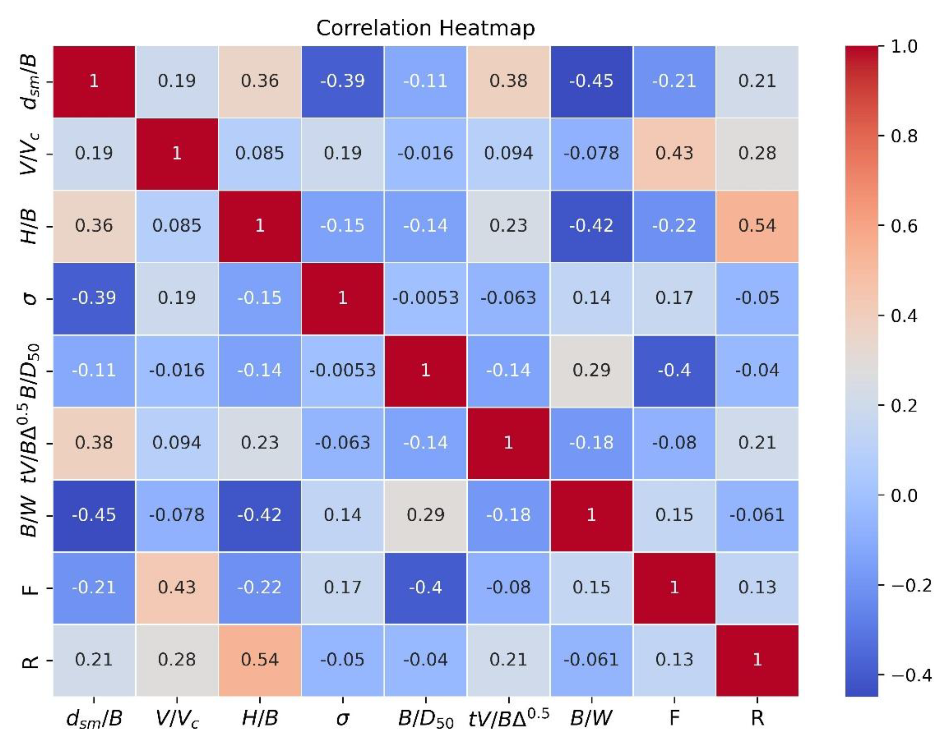
Figure 2.
New methodology designed to perform the present study.
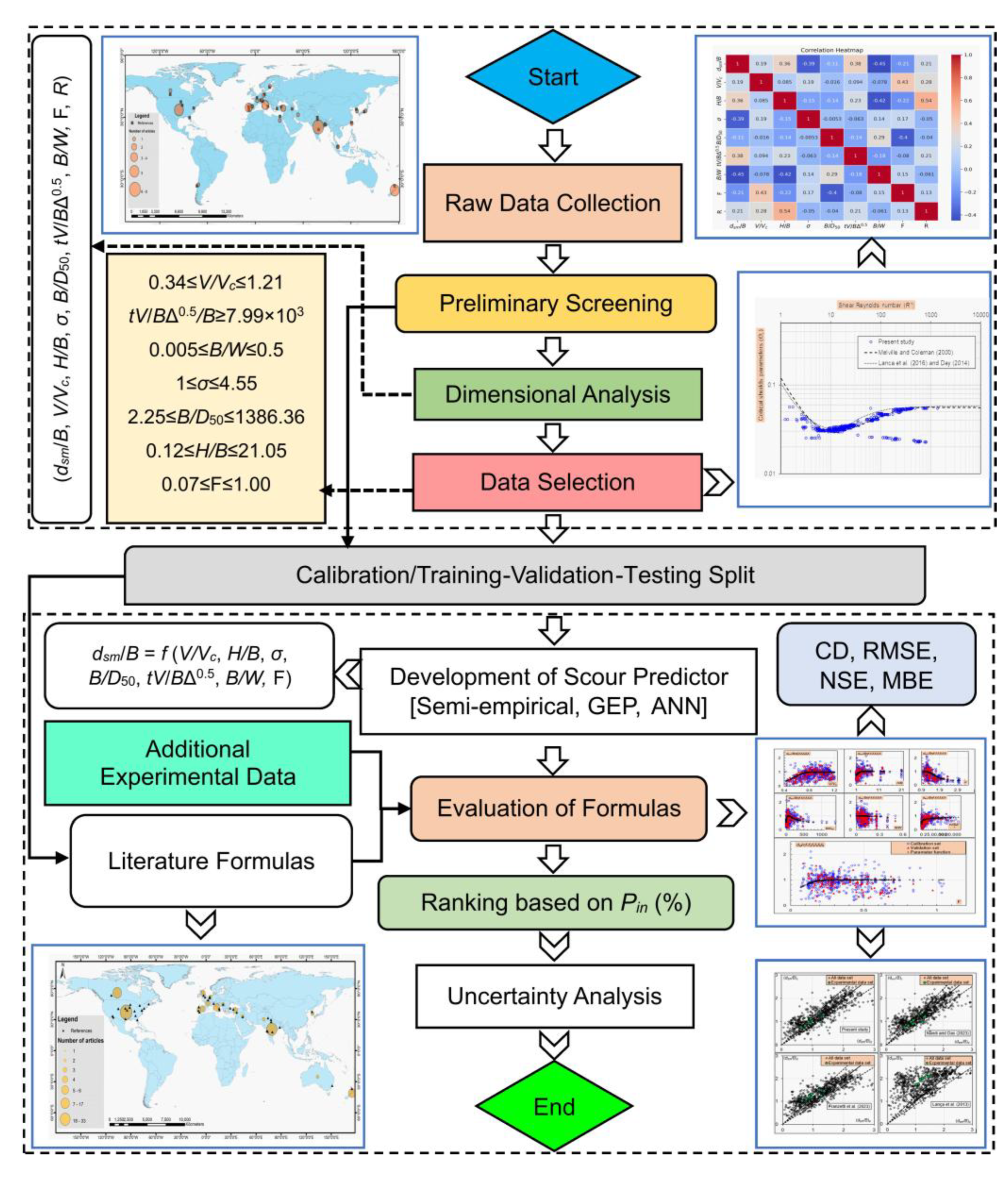
Figure 3.
Machine learning models illustrating (a) flow chart for GEP Ferreira [94], and (b) architecture for FFNN.
Figure 3.
Machine learning models illustrating (a) flow chart for GEP Ferreira [94], and (b) architecture for FFNN.
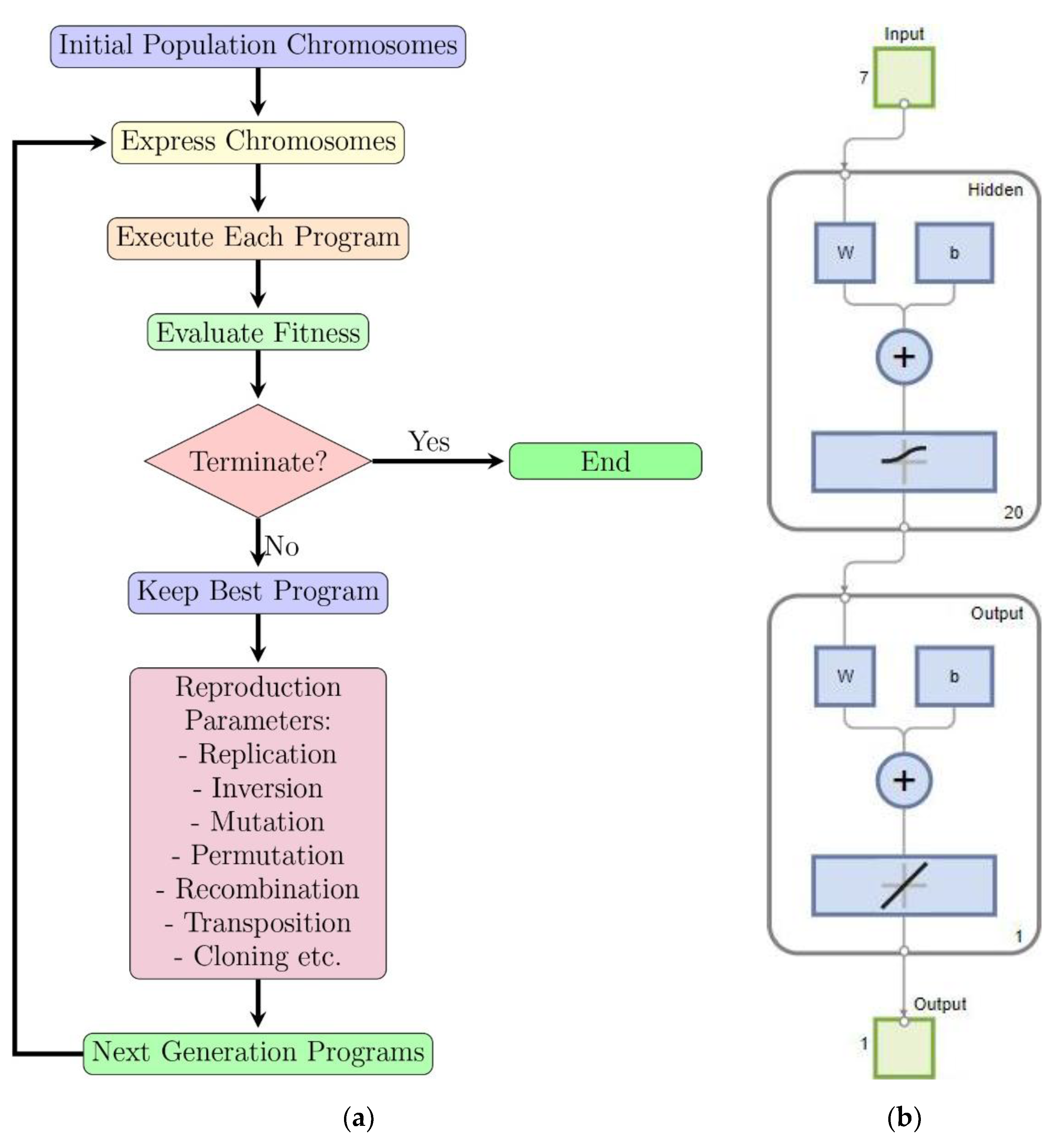
Figure 4.
The dependence of optimized parameter function (a) f1 (V/Vc); (b) f2 (H/B); (c) f3 (σ); (d) f4 (B/D50); (e) f5 (tV/BΔ0.5); (f) f6 (B/W); and (g) f7 (F).
Figure 4.
The dependence of optimized parameter function (a) f1 (V/Vc); (b) f2 (H/B); (c) f3 (σ); (d) f4 (B/D50); (e) f5 (tV/BΔ0.5); (f) f6 (B/W); and (g) f7 (F).
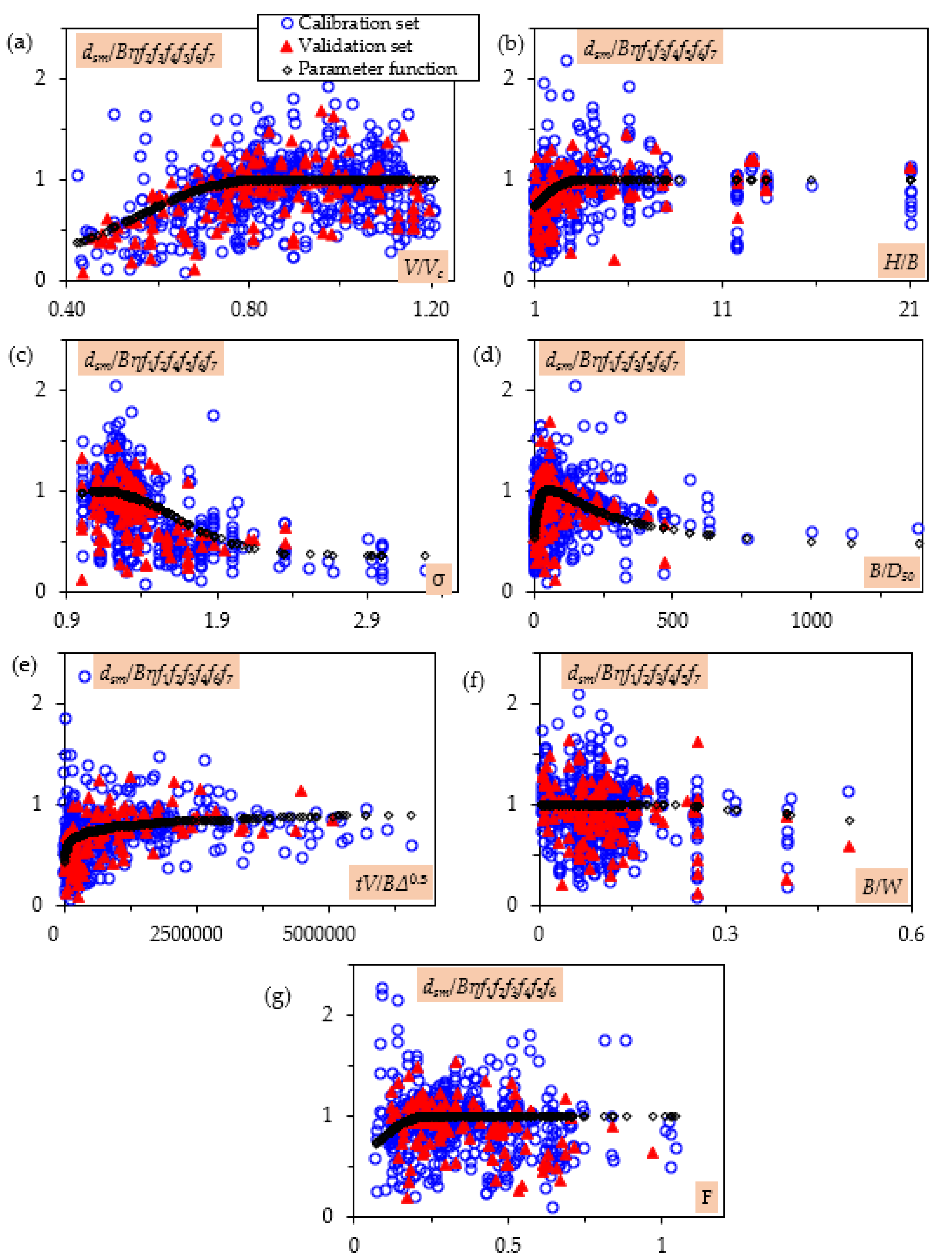
Figure 5.
Visual representation of GEP formulations in terms of expression trees.
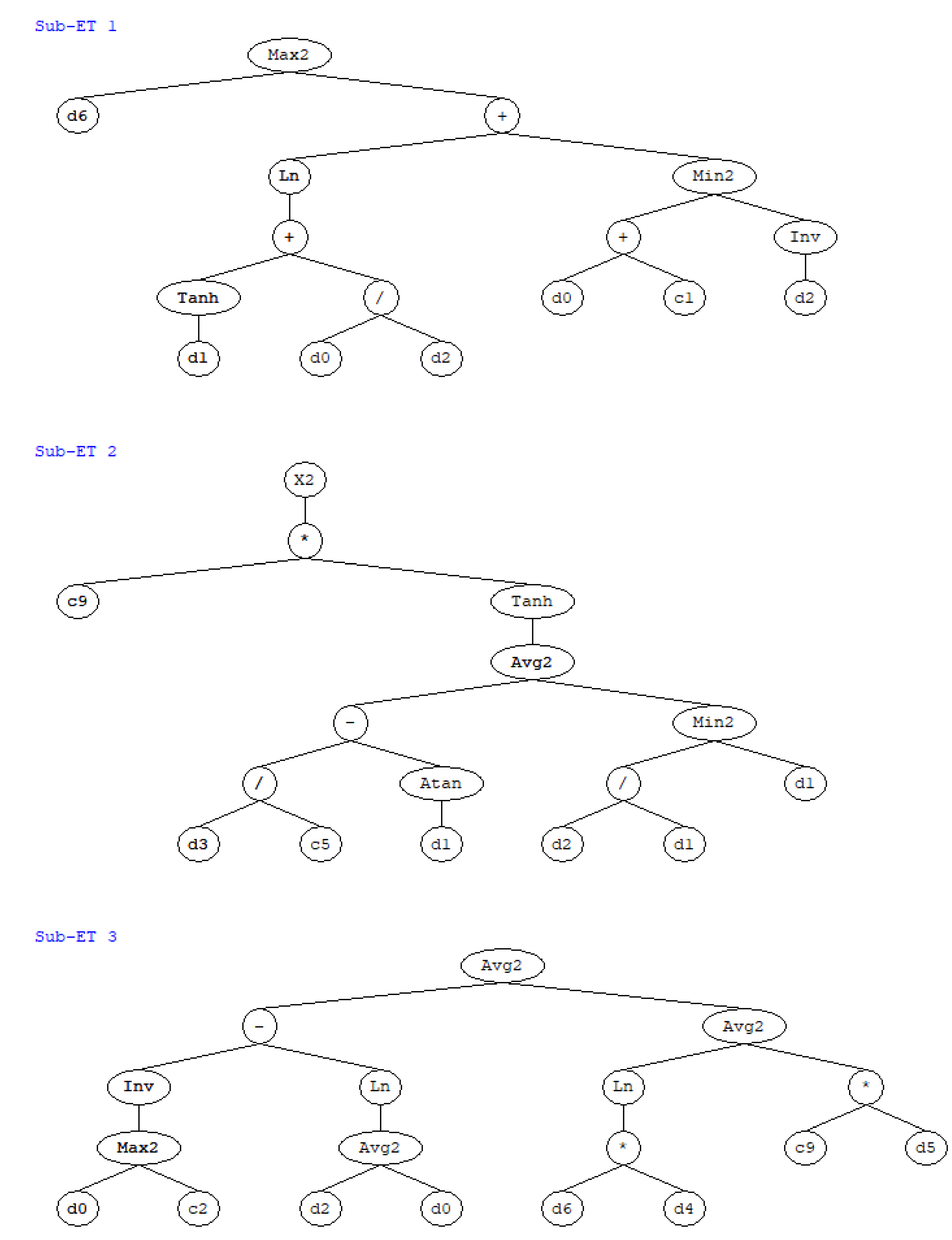
Figure 6.
Figure 6. Learning curves and the training progress of FFNN.
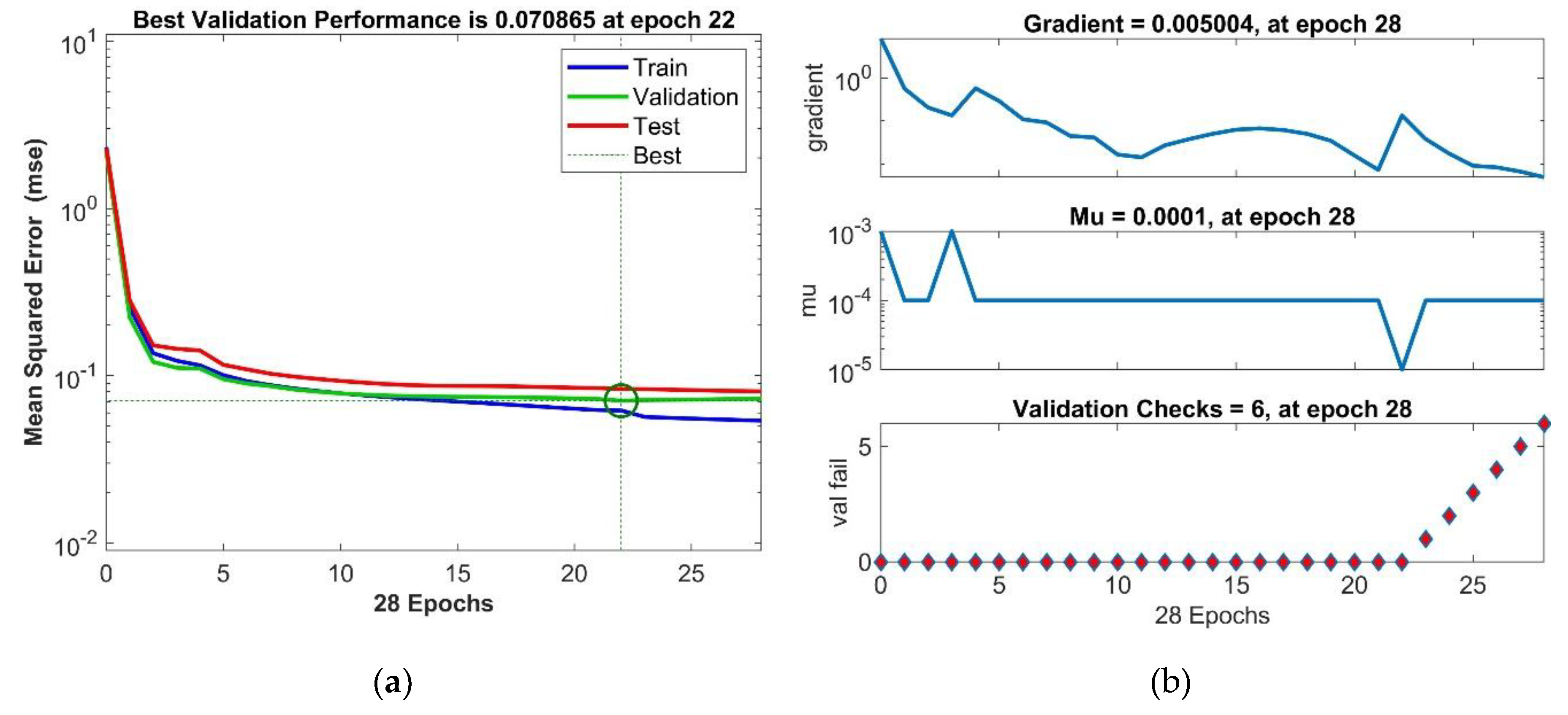
Figure 7.
Scatter diagrams for FNN in training, testing, validation, and overall data.
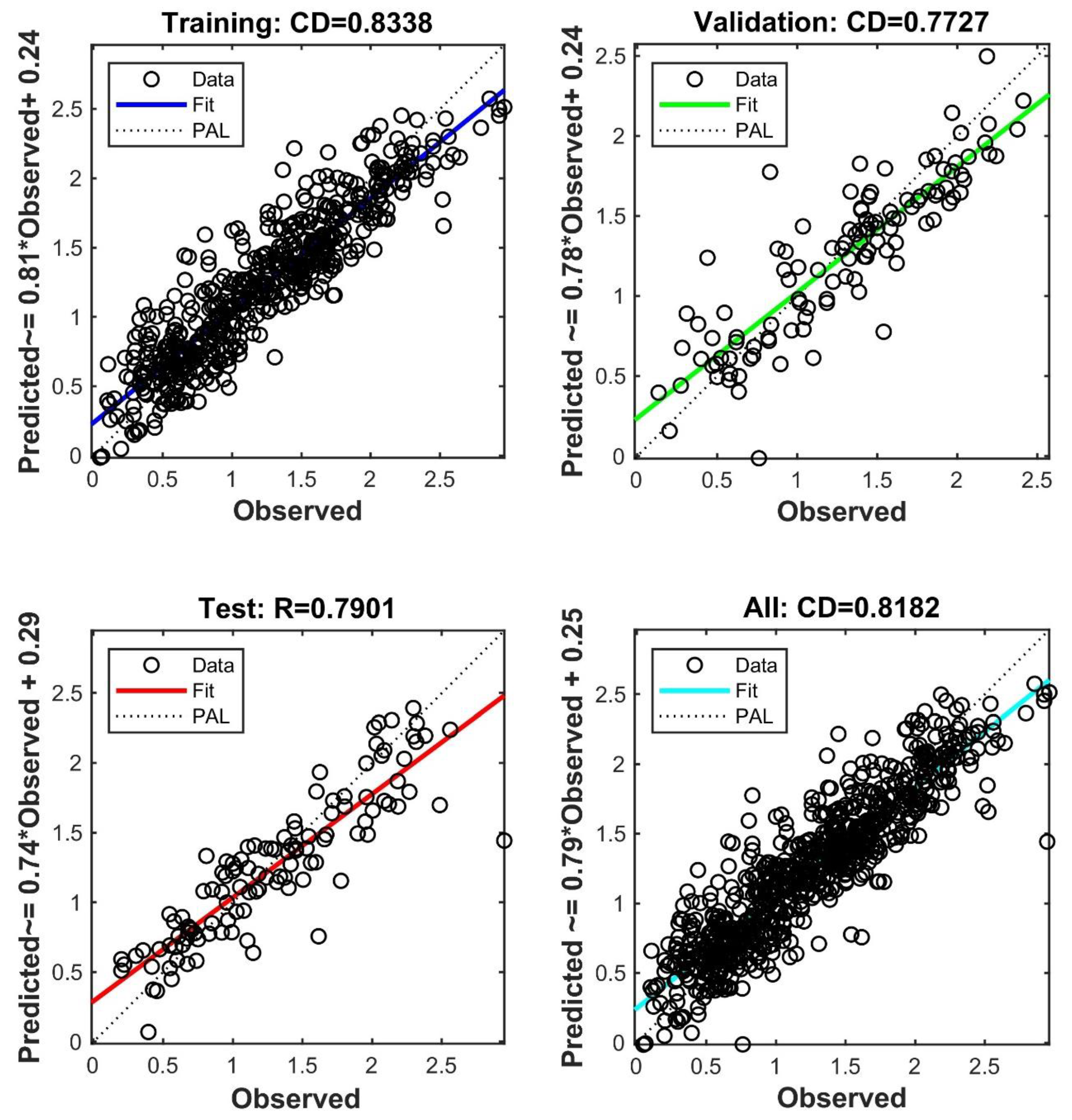
Figure 8.
Histogram of errors for the developed FFNN.
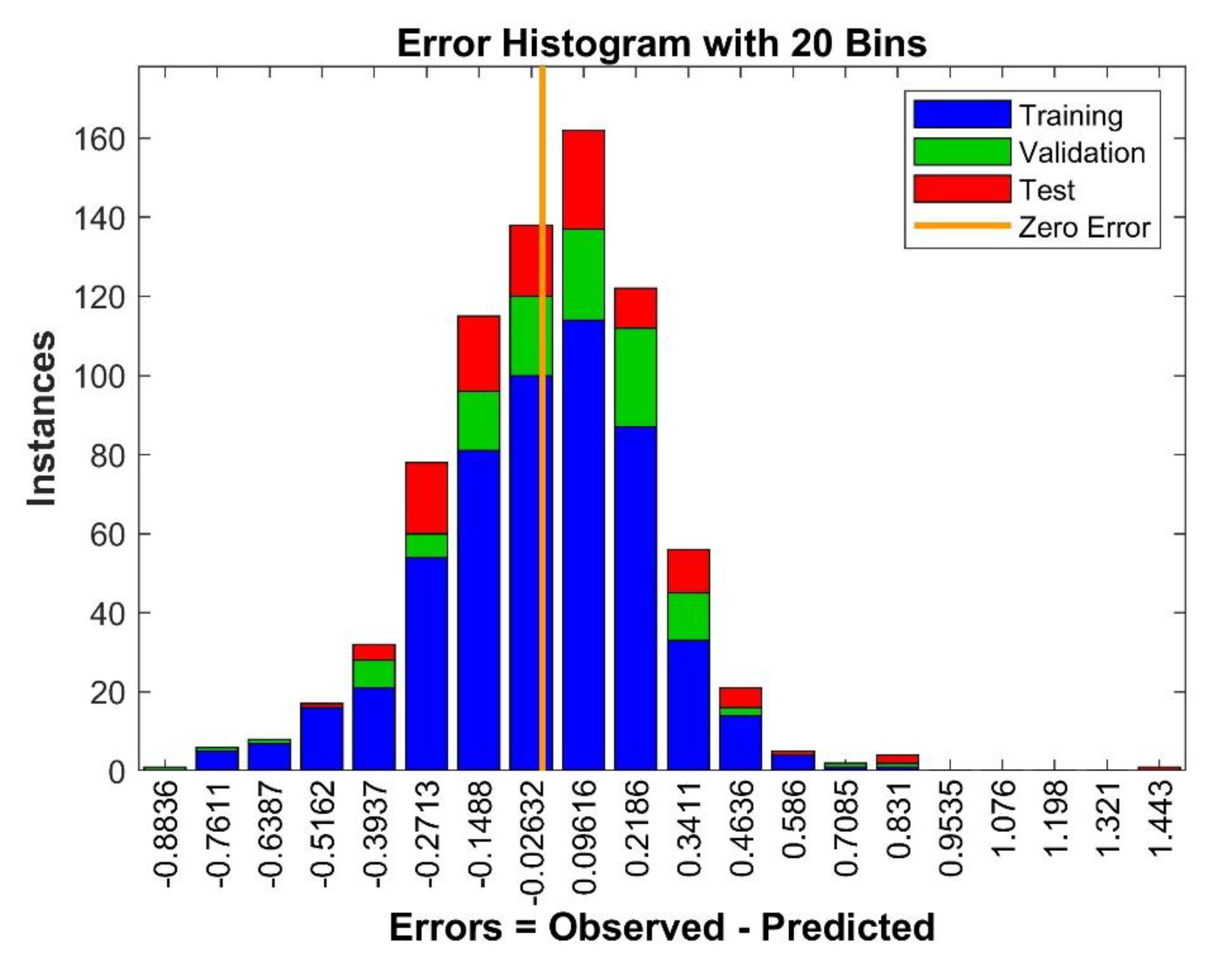
Figure 9.
Comparison between the measured and computed dsm/B using all literatures and present experimental datasets. Here, PAL is denoted by blue solid line, and ± 20% error band is shown using the red dashed line.
Figure 9.
Comparison between the measured and computed dsm/B using all literatures and present experimental datasets. Here, PAL is denoted by blue solid line, and ± 20% error band is shown using the red dashed line.
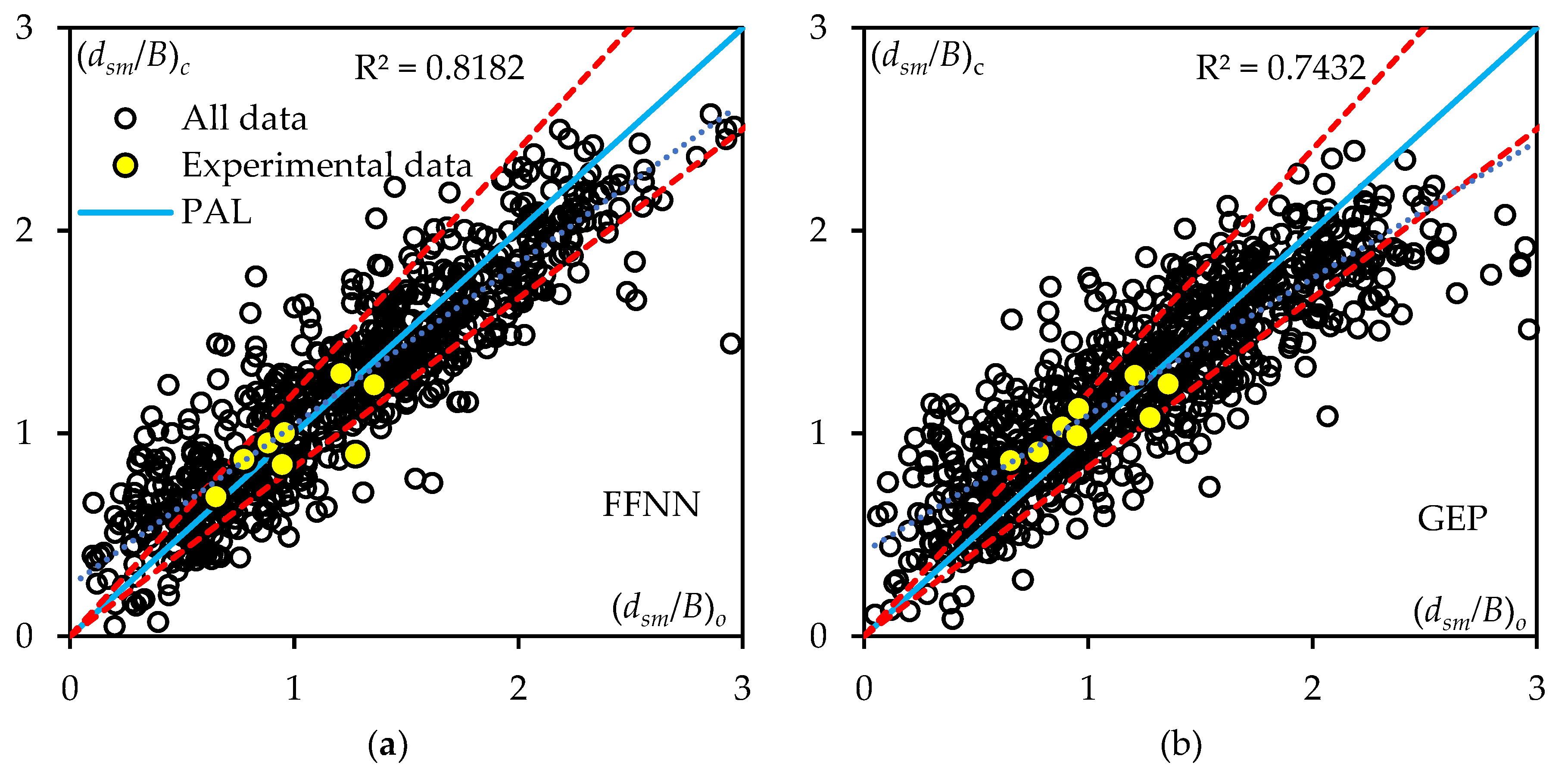
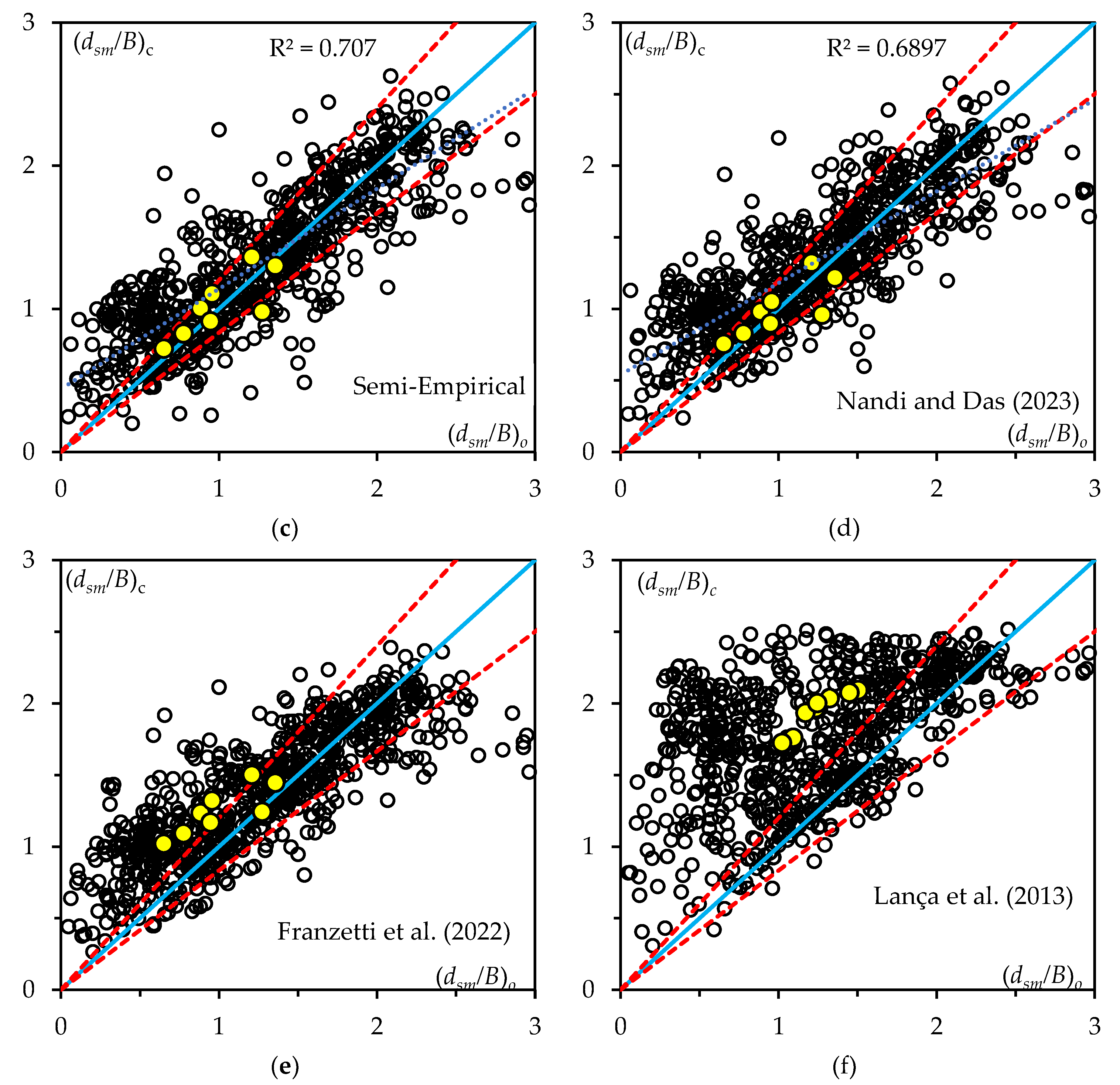
Figure 10.
Comparison of overall predicted data across six best-ranked models with observed data using box-violin plot {Present study (FFNN), Present study (Semi-Empirical), Present study (GEP), Nandi and Das [15], Franzetti et al. [14], and Lança [13]}.
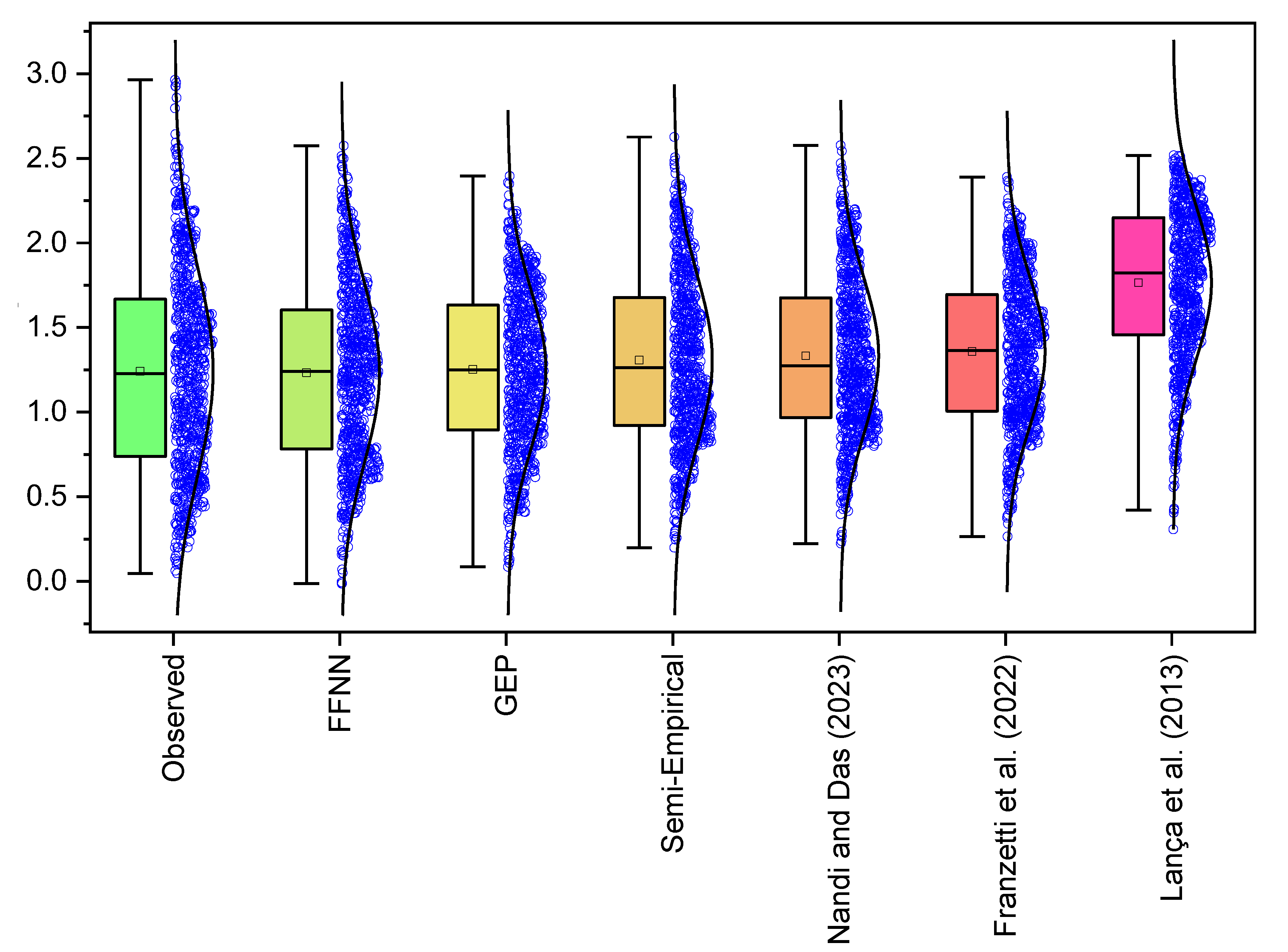
Figure 11.
Taylor diagram illustrating the performance of models across the entire dataset.
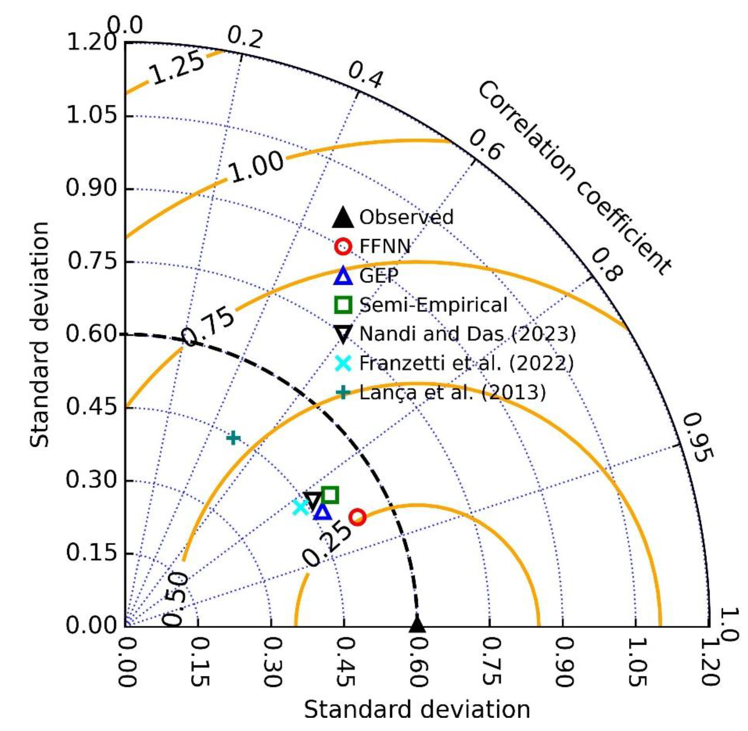

Table 1.
Definition of parameters used for the formulation of GEP.
| Parameter | Value | Parameter | Value |
| Chromosomes | 40 | Tail Size | 11 |
| Genes | 3 | Dc Size | 11 |
| Head Size | 10 | Gene Size | 32 |
| Linking Function | Multiplication (×) | ||
| Function used | Symbol | Weight | Arity |
| Addition | + | 4 | 2 |
| Subtraction | - | 4 | 2 |
| Multiplication | * | 4 | 2 |
| Division | / | 1 | 2 |
| Exponential | Exp | 1 | 1 |
| Natural logarithm | Ln | 1 | 1 |
| x to the power of 2 | X2 | 1 | 1 |
| Cube root | 3Rt | 1 | 1 |
| Arctangent | Atan | 1 | 1 |
| Minimum of 2 inputs | Min2 | 1 | 2 |
| Maximum of 2 inputs | Max2 | 1 | 2 |
| Average of 2 inputs | Avg2 | 4 | 2 |
| Hyperbolic tangent | Tanh | 1 | 1 |
| Complement | NOT | 1 | 1 |
| Inverse | Inv | 1 | 1 |
| Genetic Operator | Value | Genetic Operator | Value |
| Custom Mutation | 0.0012 | Gene Recombination | 0.00755 |
| Function Insertion | 0.00206 | One-Point Recombination | 0.00277 |
| Leaf Mutation | 0.00546 | Two-Point Recombination | 0.00277 |
| Biased Leaf Mutation | 0.00546 | Gene Recombination | 0.00277 |
| Conservative Mutation | 0.00364 | Gene Transposition | 0.00277 |
| Conservative Function Mutation | 0.00546 | Random Chromosomes | 0.0026 |
| Permutation | 0.00546 | Random Cloning | 0.00102 |
| Conservative Permutation | 0.00546 | Best Cloning | 0.0026 |
| Biased Mutation | 0.00546 | RNC Mutation | 0.00206 |
| Inversion | 0.00546 | Constant Fine-Tuning | 0.00206 |
| Tail Mutation | 0.00546 | Constant Range Finding | 0.000085 |
| Tail Inversion | 0.00546 | Constant Insertion | 0.00123 |
| IS Transposition | 0.00546 | Dc Mutation | 0.00206 |
| RIS Transposition | 0.00546 | Dc Inversion | 0.00546 |
| Stumbling Mutation | 0.00141 | Dc IS Transposition | 0.00546 |
| Recombination | 0.00755 | Dc Permutation | 0.00546 |
| Combination | Gene Number | Constant | Value |
| G1C1 | G1 | C1 | -0.0379 |
| G2C9 | G2 | C9 | 0.6467 |
| G2C5 | G2 | C5 | -5.9929 |
| G3C9 | G3 | C9 | -18.7964 |
| G3C2 | G3 | C2 | 0.8306 |
Table 2.
Performance indicators of semi-empirical, GEP, and FFNN for different datasets.
| Model | Reference datasets | Performance indicators | ||||
|---|---|---|---|---|---|---|
| CD | NSE | MBE | RMSE | Pin (%) | ||
| Empirical | Training/calibration data (80%) | 0.694 | 0.684 | 0.061 | 0.271 | 60.848 |
| Validation data (20%) | 0.756 | 0.750 | 0.089 | 0.301 | 61.935 | |
| Present Exp. data | 0.651 | 0.637 | 0.020 | 0.140 | 87.500 | |
| GEP | Training/calibration data (80%) | 0.743 | 0.738 | 0.018 | 0.246 | 61.301 |
| Validation data (20%) | 0.742 | 0.727 | -0.020 | 0.342 | 50.323 | |
| Present Exp. data | 0.737 | 0.603 | 0.060 | 0.147 | 77.778 | |
| FFNN | Training/calibration data (70%) | 0.834 | 0.833 | 0.005 | 0.249 | 65.677 |
| Validation data (15%) | 0.773 | 0.767 | -0.040 | 0.266 | 75.000 | |
| Test data (15%) | 0.790 | 0.783 | -0.039 | 0.289 | 64.655 | |
| Present Exp. data | 0.583 | 0.562 | -0.031 | 0.154 | 87.500 | |
Disclaimer/Publisher’s Note: The statements, opinions and data contained in all publications are solely those of the individual author(s) and contributor(s) and not of MDPI and/or the editor(s). MDPI and/or the editor(s) disclaim responsibility for any injury to people or property resulting from any ideas, methods, instructions or products referred to in the content. |
© 2025 by the authors. Licensee MDPI, Basel, Switzerland. This article is an open access article distributed under the terms and conditions of the Creative Commons Attribution (CC BY) license (http://creativecommons.org/licenses/by/4.0/).
Copyright: This open access article is published under a Creative Commons CC BY 4.0 license, which permit the free download, distribution, and reuse, provided that the author and preprint are cited in any reuse.


