
Submitted:
14 July 2025
Posted:
15 July 2025
You are already at the latest version
Abstract
Presently, fractal geometry serves as a framework for studies of complex systems of diverse nature. One of the most fundamental geometric conceptions is the concept of symmetry. Different geometries can be classified according to the group of transformations under which their propositions remain true. In particular, the key symmetries of the fractal geometry are the
5 scale and conformal invariance. Another key paradigm in the fractal geometry is that different properties of a fractal pattern are associated with different dimension numbers, at least one of which differs fromthe topological dimension. Accordingly, the inherent features of a fractal pattern are characterized by a set of generally independent dimension numbers. These numbers allow for the classification of fractal patterns. In this review we briefly survey the historical background and the conceptual foundations of fractal geometry.
Keywords:
fractals
; scale invariance
; conformal invariance
; dimension numbers
; degrees of freedom
1. Introduction
Geometry provides a formal representation of shapes in space. Fractal geometry deals with objects called fractals. The notion of fractals was put forward by a Polish-born French-American mathematician Benoit Mandelbrot in reference to irregular but scale invariant patterns that he studied [1]. The word fractal came from a Latin word fractus meaning broken or fractured. Although there is no canonical definition of fractals, the fractal can be defined as a scale and/or conformally invariant pattern whose dimension linked to a suitable defined measure D strictly exceeds the topological dimension d, which is defined regarding the way how the pattern can be divided into parts of arbitrary sizes [2].
The topological dimension d is a topological invariant, whereas the dimension number D, commonly called the fractal dimension, is not necessary invariant under homeomorphic transformations. For Euclidean patterns , the fractals are characterized by per definition [3]. However, the dimension number D along is insufficient for fractal characterization. Indeed, the fractal patterns having the same D can possess very different topological, morphological, and topographical properties [2,3,4,5]. Nonetheless, the inherent features of fractals can be specified by a set of generally independent dimension numbers [2,6]
Another constitutive property of fractals is their invariance under suitable defined scale and/or conformal transformations. In Figure 1 we present the corresponding classification of fractal patterns. The scale invariant fractals look the same under some sort of scaling operations. Specifically, a self-similar fractal is invariant under an appropriate similarity transformation, whereas a self-affine fractal is invariant under a suitable affine transformation (see, for instance, illustrations in Figure 1). Besides there are the hierarchical fractals which are only locally scale invariant. The difference between the scale invariant and locally scale-invariant fractals is illustrated by Figure 2. Finally, a self-conformal fractal is invariant under a special conformal transformation which locally looks as the scale one (see, for example, the illustration in Figure 1). Accordingly, the self-conformal fractals are also scale-independent, but in a stronger sense than the scale invariant fractals.
Although the term fractal was appeared only in 1975, a recursive self-similarity was already studied in the 17th century by a German mathematician and philosopher Gottfried von Leibniz (see Ref. [7] and references therein). In his celebrated letter to Guillaume de L’Hôpital von Leibniz introduced the notion of fractional exponent associated with the recursive self-similarity. Furthermore, the mathematical foundations of fractal geometry and most of paradigmatic fractals were created a long time before than the word fractal was invented by Mandelbrot (see, for review, Refs. [6,7,8,9,10,11] and references therein). Namely, several important concepts of fractal geometry have their origins in analytical and geometric constructions of nineteenth or early to mid-twentieth century.
In this review we briefly survey the historical background and conceptual foundations of fractal geometry. The rest of the paper is organized as follows. Section 2 is devoted to the history of fractal geometry creation. The conceptual foundations of the fractal geometry are highlighted in Section 3. Some key issues are outlined in Section 4.
2. Brief Excursion into the History of Fractal Geometry
In 1872 a German mathematician Karl Weierstrass has presented a function
where a is an odd integer, and . This function is everywhere continuous but nowhere differentiable, if . In his seminal paper [12] Weierstrass also stated that Georg Friedrich Bernhard Riemann was the first (in 1861) to assert that the infinite series is continuous but not differentiable. However, it is not clear whether the non-differentiability was proved by Riemann or not. The Weierstrass work shocked the mathematical community, but the continuous nowhere differentiable functions remained considered as rare pathologies for a long time. Presently, the existence of continuous nowhere differentiable functions is crucial to our proper understanding of mathematical analysis [13]. In particular, the nowhere-differentiability in the conventional sense is inherent feature of at almost all fractals. The graph of Weierstrass function is shown on in Figure 3). One can see that it exhibits a fine structure at all scales of observation, such that a smaller scale blow-up looks broadly similar to the wider plot. So, the Weierstrass graph possesses some form of approximate self-symmetry which is presently known as the self-affinity [3,14,15,16].
One of the students attending the Weierstrass’lectures was Georg Cantor who later becomes a famous mathematician. In 1883 Georg Cantor [17] explored a set of points lying on a single line segment which can be presented as
where is 0 or 2 for each integer k. Although the same set was early studied by Henry John Stephen Smith [18], it was named as the Cantor set since through consideration of this set Cantor helped to lay the foundations of modern point-set topology [19]. The Cantor set is an example of uncountable bounded sets that have zero one-dimensional Lebesgue measure (length). It has been also recognized that the Cantor set is a subset of Euclidean space which is perfect (a closed set that contains no isolated point) but nowhere dense in any interval, regardless of how small the interval is taken to be (closure has empty interior). Geometrically, the middle third Cantor set is constructed by repeatedly removing middle third open intervals from the unit interval as it is shown in Figure 4.
Due to its remarkable properties, the Cantor set plays a vital role in many branches of mathematics. In particular, its special place in the theory of compact spaces is coined by the Hausdorff–Alexandroff theorem which states that any compact metric space is a continuous image of the Cantor set [20]. In the fractal geometry the Cantor set constitutes the class of totally disconnected fractals (see, for review, Refs. [21,22,23] and references therein).
In the last part of 19 century, Felix Klein and Henri Poincaré introduced a category of objects that we now call the self-inverse fractals (see, for example, the construction of self-conformal fractal in Figure 1) and form a part of the self-conformal fractals (see, for review, Refs. [24,25,26,27]). Furthermore, self-inverse fractals have become a special topic of the theory of automorphic functions (see Ref. [24] and references therein).
In 1890, an Italian mathematician and glottologist Giuseppe Peano [28] has discovered the first example of curves that passes through every point of a two-dimensional region having a positive Jordan area (see in Figure 5a). Immediate1y after that a German mathematician David Hilbert [29] replaced the purely arithmetic definition proposed by Peano on a more descriptive geometric construction of graphs and thus built up a celebrated variant of Peano curve (see in Figure 5b). Later there were constructed non-intersecting continuous curves filling the n-dimensional spaces. Presently the class of space-filling curves is also called the Peano curves [30,31,32].
In 1904, a Swedish mathematician Niels Fabian Helge von Koch [33] has devised the simplest variant of continuous curve without tangents (see Fig. 6), which is now called the Koch curve. Koch has showed that there exists a parameterization of the curve for , where both functions and are continuous but nowhere differentiable. The Koch curve challenges our notion of a curve. While the curve is connected and contained in a bounded region of the plane its length is infinite. Moreover, any part of the Koch curve has infinite length (see Figure 6a). Fitting together three suitably rotated copies of the curve produces a snowflake curve (see Figure 6b), sometimes also called the Koch island [34]. In the fractal geometry Koch curves constitute the class of self-avoiding self-similar fractals (see, for review, Refs. [34,35,36] and references therein). Figure 6c shows the construction of Koch curve starting from a triangle.
In 1912 by a Polish mathematician Wacław Sierpiński [37] has presented the most famous space-filling curve nowadays called the Sierpiński square snowflake (see Figure 5c). So it was revealed a continuous crossover between the Koch and Peano curves [38]. In 1918 two French mathematicians Pierre Fatou and Gaston Julia found a self-similar behavior associated with mapping complex numbers and iterative functions [39,40,41]. The idea of self-similar curves was taken further by Paul Pierre Lévy, who, in 1938, created a self-similar curve, presently known as the Lévy C curve [42]. In 1915 Sierpiński [43] has devised a self-similar curve having almost all points as the branching points. This curve, known as the Sierpiński gasket was constructed by deleting an open middle triangle from a closed equilateral triangle of unit side and by repeating this step for the remaining sub-triangles ad infinitum (see Figure 7a). Later Sierpiński [44,45] also proposed to create the same shape as the limit of the Koch-like arrowhead curve (see Figure 7b). However, in contrast to the Sierpiński gasket with loops at all scales, the Sierpiński arrowhead curve remains loopless even in the limit of infinite number of iterations [46]. Further there were suggested many other ways to create the Sierpiński triangle shape (see, for review, Refs. [47,48,49] and references therein). Nowadays the Sierpinski triangle is one of the most studied fractal shapes.
In 1916 Sierpiśki [50] constructed a curve forming an infinitely ramified network (see Figure 8) nowadays known as the Sierpiński carpet. Analogous curve in three dimensions was presented by Karl Menger in 1926 [51]. Notice that the Sierpiński carpet and the Menger sponge can be viewed as the analogs of Cantor set on the plane and in the three dimensional space, respectively (see, for review, Ref. [21]).
On the other hand, in 1918 Felix Hausdorff [52] has introduced a new definition of covering measure based on the set size variations with the scale of measurements. The dimension number D associated with that measure, presently called the Hausdorff dimension, can be fractional. In particular, Hausdorff proved that the middle-third Cantor set is characterized by fractional dimension . Further, the conceptual and technical aspects regarding the Hausdorff measure and dimension were disused by Besicovitch [53,54]. In 1968 a biologist Aristid Lindenmayer [55] invented an approach for simulating the development of multicellular organisms, subsequently named L-systems [56]. The central concept of the Lindenmayer system is that of re-writing. This approach was specifically created for the description of natural growth processes and so enables us to see in more detail how a fractal grows (see, for example, Figure 2b). Accordingly, the L-systems represent a large class of real-world fractals in a mathematical way [57].
In this background Benoit Mandelbrot published his celebrated paper [58] in which he resolved the Steinhaus Paradox that the measured length of geographic features increases with increasing map scales. Sometime afterward, Mandelbrot [1] coined the notion of fractals to define a large class of mathematical and natural objects that possess the property of scale invariance whose covering dimension strictly exceeds the topological one. In a unified way, the scale-invariant fractals were created by John Hutchinson [59] using the method of Iterated Function Systems (IFS). Further, the IFS method was popularized by Barnsley [60] as a generalization of the Banach contraction principle. In the late 20th century fractals became a topic of rising interest for researchers specializing in diverse areas of mathematics, physics, and natural sciences (see, for instance, Refs. [61,62,63,64,65,66,67,68,69,70,71,72] and references therein). Presently, the fractal geometry still remains a burgeoning area of research (see, for review, Refs. [73,74,75,76,77,78,79,80,81,82,83,84,85,86,87,88,89,90,91,92,93,94,95,96,97,98,99,100,101,102,103] and references therein).
3. Conceptual Foundations of Fractal Geometry
The fractal geometry deals with intricate patterns and irregular shapes possessing the scale and/or conformal symmetry. In this regard, it is pertinent to note that the scale symmetry is an inherent feature not only of fractals, but also of the small-world and scale-free networks, as well as of the objects with a power-law size distribution of the building blocks (see Figure 9). Geometrically, the scale invariance is associated with the notion of self-similarity or self-affinity, which can be exact (deterministic) or approximate (statistical). Besides, there are self-conforming fractals that are invariant under special conformal transformations.
The scale invariance can be characterized by the similarity dimension defined via the Hutchinson–Moran formula
where are the contraction ratios and m is the number of contractions at each iteration step [59]. For scale invariant Euclidean patterns the similarity dimension is equal to the topological one (that is ), whereas for fractals per definition. The topological dimension is defined inductively as follows. Let us an empty space has the topological dimension . A pattern has the topological dimension zero if for any point of it there exist arbitrarily small neighborhoods whose boundary is empty. A pattern has the topological dimension if there are arbitrarily small neighborhoods of any point whose boundary is of dimension , where n is a natural number.
An equivalent recursive definition of topological dimension reads as:
while it is assumed that [104]. So, the topological dimension stipulates a way to divide an object into parts of arbitrary sizes. Furthermore, in the Euclidean geometry, the topological dimension d also:
- 1)
- handles the scale invariance of the Euclidean object ;
- 2)
- characterizes the object connectivity;
- 3)
- establishes the object ramification;
- 4)
- sets the maximum number of mutually orthogonal vectors in the object;
- 5)
- governs the Lebesgue measure and other Borel measures on Euclidean space;
- 6)
- determines the numbers of spatial and dynamic degrees of freedom of a point walker in the object
- 7)
- rules the statistics of thomogeneous Poisson point processes;
- 8)
- controls the vibrational dynamics of the object;
- 9)
- manages the information flow;
- 10)
- settles the values of universal exponents associated with critical phenomena.
Conversely, in the fractal geometry, the above features are associated with a set of different dimensional numbers, some of which are topological invariants and others are not. Specifically, the similarity dimension defined by Eq. (2) can be linked to a suitable defined covering measure, e.g. the Hausdorff, box-counting, packing, or Assouad measure (see, for review, Table 1 and Figure 10. In this way, it was recognized that the similarity and Hausdorff dimensions are equivalent when the IFS satisfies the open set condition [64]. Therefore the fractal dimension can be thought of as a measure of a pattern’s ability to fill the space in which it resides. The scale invariance implies that the number of boxes needed to cover a fractal pattern scales with the box size as . Accordingly, the fractal dimension is frequently defined through the scaling relation , where is the scale factor [17].
In contrast to the topological dimension, the fractal dimension is not a topological invariant. Accordingly the topological features of fractals (see Figure 11) can be characterized by a set of dimension numbers which generally differ from the fractal and topological dimensions [2].
Specifically, the pattern’s connectivity can be quantified by the connectivity dimension defined as:
where is the number of pattern’s points connected with an arbitrary point inside of the -ball of diameter l [105]. Accordingly, the connectivity dimension of the fractal network is equal to
where is the network diameter defined as the maximum geodesic distance between two sites on the network, while is the Wiener index and is the minimum number of steps needed to go from site x to site y on the network F [97]. It is a straightforward matter to understand that the ratio of the fractal and connectivity dimensions is equal to the fractal dimension of geodesic paths [2]. That is the fractal dimension of geodesic paths is equal to
Accordingly, fractals can be either of the metric origin, if (see, for instance, Figure 12a), or of the topological origin, if (see Figure 12b). Furthermore, fractals can have combined origin, such that (see, for example, Figure 12c).
A point-like random walker on a Euclidean pattern has equal numbers of spatial and dynamical degrees of freedom. Both are equal to the topological dimension of the pattern. In contrast to this, for fractal patters the number of effective dynamical degrees of freedom can be equal to or less than the number of effective spatial degrees of freedom [106]. The number of effective dynamical degrees of freedom is defined via the scaling asymptotic behavior of the probability that the random walker returns to its origin point after t steps (), while the number of effective spatial degrees of freedom can be viewed as the number of independent directions under a constrain imposed by the fractal topology. In Ref. [106] it has been established that
while the number of effective dynamical degrees of freedom of the point-like random walker is equal to the spectral dimension of the fractal pattern. The Einstein law relating the drift and diffusion of charge implies that
where is the random walk dimension and is the electrical resistance exponent defined via the scaling relations if , or , if [107]. Furthermore, many kinds of fractals obey the Alexander-Orbach relation and so the electrical resistance exponent is equal to [61,62,63].
Scale invariant fractals can be loopless (see, for example, fractals in Figure 12) or have loops at all scales (see, for example, fractals in Figs. Figure 7 and Figure 8). For the loopless fractals . Consequently, the spectral dimension of a loopless fractal is equal to
whereas for fractals with loops at all scales the spectral dimension is in the range of
Accordingly, the fractal loopiness can be characterized by the loopiness index which was defined in Ref. [2] as
while for the loopless fractals () the spectral dimension is equal to and loopy fractals () have .
Another important property of patterns is their ramification. Quantitatively, the order of ramification at point j on the pattern is defined as the smallest number of bonds that should be cut in order to isolate an arbitrarily large bounded set of points connected to the point j. Then the order of pattern ramification is defined as [108]:
Finitely ramified patterns have the finite orders of ramification, whereas the order of ramification of an infinitely ramified pattern grows with the size L of as , such that , as . Accordingly the order of ramification is characterized by the ramification exponent
while for the finitely ramified patterns . In Ref. [109] it was recognized that the ramification exponent can be related to the topological Hausdorff dimension which was introduced in [104] via a combination of the definitions of the topological and Hausdorff dimensions:
Further, it was argued that this definition can be generalized to define the topological fractal dimension with the use of any suitable fractal dimension (see, for instance, Table 1) instead of the Hausdorff one. The topological fractal dimension is related to the ramification exponent as [109]. Generally, , while for Euclidean patterns [2].
Likewise the fractal dimension the topological fractal dimension is not topologically invariant. The topological invariant associated with the fractal ramification was introduced in Ref. [81] and named the topological connectivity dimension. It is defined as
where is the fractal dimension of the subset S with respect to the geodesic metric on the pattern . The infinitely ramified patterns are characterized by , whereas the finitely ramified patterns have [2].
4. Final Remarks
Fractal geometry is a relatively new branch of mathematics that was launched in the 1970’s. Since then, it has been linked to many branches of mathematics, including number theory, topology, differential geometry, statistics, operator algebras, potential theory, mathematical physics, harmonic analysis, and the theory of dynamical systems. Presently, the fractal geometry remains an active area of development. In particular, many works were focused on the inherent features of fractal patterns. The morphological properties of scale invariant patterns were reviewed in Ref. [5]. The topographical attributes of fractals were discussed in details in Ref. [2]. In this review we discuss the topological features of fractal patterns. The pattern’s topology can be characterized by calculating so-called topological invariants. The topological invariants fix certain topological features such as the number of connected components, the pattern connectivity and ramification, the existence and distribution of holes and knots in the studied pattern. We state that the fractal loopiness can be characterized by the ratio between the numbers of effective spatial and effective dynamical degrees of freedom on the fractal. However, an appropriate characterization of the fractal knottedness remains open (see Refs. [113,114,115] and references therein).
In nature, complex irregular and fragmented patterns arise in a wide variety of systems. The main appeal of fractal geometry is its ability to describe complex patterns that traditional Euclidean geometry is unable to analyze. Accordingly, fractal geometry has become one of the powerful tools for image analysis in many fields of science, including computer science, physics, mechanical and electrical engineering, biophysics, medicine and economics, and others.
Author Contributions
D.S.O.—writing, discussion, review; E.I.G.O.—data curation, visualization, discussion; A.S.B.—conceptualization, discussion, supervision.
Funding
This research was sponsored by the Instituto Politécnico Nacional Project under research grants 20250564 and 20250854
Institutional Review Board Statement
Not applicable.
Informed Consent Statement
Not applicable.
Data Availability Statement
All data are contained within the paper, and a report of any other data is not included.
Acknowledgments
The second author would like to express gratitude to the SECIHTI: I1200/111/2024 scholarship for postdoctoral studies
Conflicts of Interest
The authors declare no conflict of interest.
References
- Mandelbrot, B.B. Fractals: Form, Chance, and Dimension. Freeman: New York, 1977.
- Balankin, A.S., Patiño, J., Patiño, M. Inherent features of fractal sets and key attributes of fractal models. Fractals 2022, 30, 1-23. [CrossRef]
- Mandelbrot, B.B. The Fractal Geometry of Nature. Freeman: New York, 1982.
- Balankin, A.S. Fractional space approach to studies of physical phenomena on fractals and in confined low-dimensional systems. Chaos Solitons Fractals 2020, 32, 109572. [CrossRef]
- Patino-Ortiz, J.; Martínez-Cruz, M.Á.; Esquivel-Patino, F.R.; Balankin, A.S. Morphological Features of Mathematical and Real-World Fractals: A Survey. Fractal Fract. 2024, 8, 440. [CrossRef]
- Patino-Ortiz, J.; Patino-Ortiz, M.; Martínez-Cruz, M.-Á.; Balankin, A.S. A Brief Survey of Paradigmatic Fractals from a Topological Perspective. Fractal Fract. 2023, 7, 597. [CrossRef]
- Nutu, C.S.; Axinte, T. Fractals. Origins and History. J. Marine Tech. Envir. 2022, 2, 48-51. [CrossRef]
- Chabert, J.L. Un demi-siecle de fractales: 1870-l920. Historia Mathematica 1990, 17(4), 339-365. [CrossRef]
- Debnath, L. A brief historical introduction to fractals and fractal geometry. Int. J. Math. Educ. Sci. Tech. 2006, 37(1), 29-50. [CrossRef]
- Kuznetsov, V.A. Historical aspects of fractal theory appearance. Physics of Wave Processes and Radio Systems 2021, 24(2), 113-126. [CrossRef]
- Husain, A.; Nanda, M.N.; Chowdary, M.S.; Sajid, M. Fractals: An Eclectic Survey, Part-I. Fractal Fract. 2022, 6, 89. [CrossRef]
- Weierstrass, K. Über Continuirliche Functionen Eines Reellen Arguments, die für Keinen Werth des Letzteren Einen Bestimmten Differentialquotienten Besitzen. In: Siegmund-Schultze, R. (eds) Ausgewählte Kapitel aus der Funktionenlehre. Teubner-Archiv zur Mathematik, vol 9; Springer: Vienna, 1988. [CrossRef]
- Pinkus, A. Weierstrass and Approximation Theory. J. Approx. Theory 2000, 107, 1-66. [CrossRef]
- Matsushita, M.; Ouchi, S. On the self-affinity of various curves. Physica D 1989, 38(1-3), 246-251. [CrossRef]
- Balankin, A. S. Physics of fracture and mechanics of self-affine cracks. Eng. Fract. Mech. 1997, 57(2-3), 135-203. [CrossRef]
- Barański, K.; Bárány, B.; Romanowska, J. On the dimension of the graph of the classical Weierstrass function. Adv. Math. 2014, 265, 32-59. [CrossRef]
- Cantor, G. Uber unendliche, lineare Punktmannigfaltigkeiten V. Math. Ann. 1883, 21, 545–591, Reprinted in Cantor, G. Gesammelte Abhandlungen Mathematischen und Philosophischen Inhalts; Zermelo, E., Ed.; Springer: New York, NY, USA, 1980; pp. 165–209. [CrossRef]
- Smith, H.J.S. On the integration of discontinuous functions, Proc. London Math. Soc. 1875, 1, 140-153. [CrossRef]
- Fleron, J.F. A Note on the History of the Cantor Set and Cantor Function, Math. Mag. 1994, 67(2), 136-140. [CrossRef]
- Conway, J.B. A Course in Point Set Topology; Springer: New York, 2014. [CrossRef]
- Balankin, A. S.; Bory-Reyes, J.; Luna-Elizarrarás, M. E.; Shapiro, M. Cantor-type sets in hyperbolic numbers. Fractals 2016, 24(04), 1650051. [CrossRef]
- Björn, A.; Björn, J.; Gill, J.T., Shanmugalingam, N. Geometric analysis on Cantor sets and trees. Journal für die reine und angewandte Mathematik 2017, 725, 63-114. [CrossRef]
- Das, S.K.; Mishra, J.; Nayak, S.R. Generation of Cantor sets from fractal squares: A mathematical prospective. J. Interdisciplinary Math. 2022, 25(3), 863-880. [CrossRef]
- Mandelbrot, B.B. Self-inverse fractals, Apollonian nets, and soap. In: Fractals and Chaos. Springer, New York, NY, 2004. [CrossRef]
- Yong-ping, Z.; He-ping, X. Fractal geometry derived from geometric inversion. Appl. Math. Mech. 1990, 11, 1075-1079. [CrossRef]
- Borodich, F.M. Parametric homogeneity and non-classical self-similarity. I. Mathematical background. Acta mechanica 1998, 131(1), 27-45. [CrossRef]
- Frame, M.; Cogevina, T. An infinite circle inversion limit set fractal. Comp. Graph. 2000, 24(5), 797-804. [CrossRef]
- Peano, G. Sur une courbe, qui remplit toute une aire plane, Mathematische Annalen 1890, 36, 157-160. Reprinted in Arbeiten zur Analysis und zur mathematischen Logik. Teubner-Archiv zur Mathematik, vol 13. Springer: Vienna, 1990. [CrossRef]
- Hilbert, D. Uber die stetige Abbildung einer Linie auf ein Flăchenstuck. Mathematischc Annalen 1891, 38, 459-460. Reprinted in Dritter Band: Analysis · Grundlagen der Mathematik · Physik Verschiedenes. Springer: Berlin, Heidelberg, 1935. [CrossRef]
- Yang, J.; Bin, H.; Zhang, X.; Liu, Z. Fractal scanning path generation and control system for selective laser sintering (SLS). Int. J. Mach. Tools Manuf. 2003, 43(3), 293-300. [CrossRef]
- Sagan, H. On the geometrization of the Peano curve and the arithmetization of the Hilbert curve. Int. J. Math. Education Sci. Tech. 1992, 23, 403-411. [CrossRef]
- Humke, P.D.; Huynh, K.V. Finding keys to the Peano curve. Acta Math. Hungar. 2022, 167, 255–277. [CrossRef]
- von Koch, H. Sur un e courbe continue sans tangente, obtenue par une construction geometrique elementaire. Arkiv for Matematik, Astronomi och Fysik 1904, 1, 681 - 704.
- McCartney, M. Four variations on a fractal theme. Int. J. Math. Educ. Sci. Tech. 2024, 55(9), 2374-2388. [CrossRef]
- Ri, S.I.; Drakopoulos, V.; Nam, S.M. Fractal interpolation using harmonic functions on the Koch curve. Fractal Fract. 2021, 5(2), 28. [CrossRef]
- Lyakhov, L.N.; Sanina, E.L. Differential and integral operations in hidden spherical symmetry and the dimension of the Koch curve. Math. Notes 2023, 113(3), 502-511. [CrossRef]
- Sierpifiski, W. Sur une nouvelle courbe continue qui remplit toute une aire plane. Bull Int. Acad. Sci. Cracovie A 1912, 462-478-.
- Nisha, P.S.A.; Hemalatha, S.; Sriram, S.; Subramanian, K.G. P Systems for Patterns of Sierpinski Square Snowflake Curve. Punjab Univ. J. Math. 2020, 52, 11–18. Available online: http://journals.pu.edu.pk/journals/index.php/pujm/article/viewArticle/3679.
- Alexander, D.S. Fatou and Julia. In: A History of Complex Dynamics. Aspects of Mathematics, vol. 24. Vieweg+Teubner Verlag, Wiesbaden, 1994. [CrossRef]
- Sun, W.; Liu, S. Consensus of Julia Sets. Fractal Fract. 2022, 6, 43. [CrossRef]
- Danca, MF.; Fečkan, M. Mandelbrot set and Julia sets of fractional order. Nonlinear Dyn. 2023, 111, 9555–9570. [CrossRef]
- Akhmet, M.; Fen, M.O.; Alejaily, E.M. Dynamics with chaos and fractals. Cham, Switzerland: Springer, 2020.
- Sierpinski, W. Sur une courbe dont tout point est un point de ramification. C. R. Acad. Paris 1915, 160, 302–305.
- Sierpifiski, W. On a curve every point of which is a point of ramification, Prace Mat. Fiz. 1916, 27, 77-86.
- W. Sierpifiski, Oeuvres Choisies, Warsaw: Pafiswowe Wydwnicto Naukowe, 1975.
- Martńez-Cruz, M.-Á.; Patiño-Ortiz, J.; Patiño-Ortiz, M.; Balankin, A.S. Some Insights into the Sierpinski Triangle Paradox. Fractal Fract. 2024, 8, 655. [CrossRef]
- Stewart, I. Four Encounters with Sierpinski’s Gasket. Math. Intell. 1995, 17, 52–64. [CrossRef]
- Reiter, C.; With, J. 101 ways to build a Sierpinski triangle. ACM SIGAPL APL Quote Quad. 1997, 27, 8–16. Available online: http://hdl.handle.net/10385/1842.
- Luna-Elizarrarás, M.E.; Shapiro, M.; Balankin, A.S. Fractal-type sets in the four-dimensional space using bicomplex and hyperbolic numbers. Anal. Math. Phys. 2020, 10, 13. [CrossRef]
- Sierpinski, W. Sur une courbe cantorienne qui contient une image biunivoque et continue de toute courbe donnee. C. R. Acad. Paris1916, 162, 629–632.
- Menger, K.; Brouwer, L.E.J. “Allgemeine Räume und Cartesische Räume”. Zweite Mitteilung: “Ueber umfassendste n-dimensionale Mengen”. In Selecta Mathematica. Springer: Vienna, Austria, 2002; pp. 89–92. [CrossRef]
- Hausdorff, F. Dimension und auBeres Maß. Math. Ann. 1918, 79, 157–179. [CrossRef]
- Besicovitch, A.S. Sets of Fractional Dimensions (IV): On Rational Approximation to Real Numbers. J. Lond. Math. Soc. 1934, s1–s9, 126–131. [CrossRef]
- Besicovitch, A.S.; Ursell, H.D. Sets of Fractional Dimensions (V): On Dimensional Numbers of Some Continuous Curves. J. Lond. Math. Soc. 1937, s1–s12, 18–25. [CrossRef]
- Lindenmayer, A. Mathematical models for cellular interaction in development I. Filaments with one-sided inputs. J. Theor. Biol. 1968, 18, 280-315. [CrossRef]
- Oberguggenberger, M.; Ostermann, A. Fractals and L-Systems. In: Analysis for Computer Scientists. Undergraduate Topics in Computer Science. Springer: London, 2011. [CrossRef]
- Ahmed, B. Fractal Geometry in Nature: Applications in Physics and Mathematical Theory. Frontiers in Applied Physics and Mathematics 2024, 1(2), 129-145.
- Mandelbrot, B.B. How long is the coast of Britain? Statistical self-similarity and fractional dimension. Science 1967, 156, 636–638. [CrossRef]
- Hutchinson, J.E. Fractals and self-similarity. Indiana Univ. Math. J. 1981, 30, 713–747. Available online: https://www.jstor.org/stable/24893080.
- Barnsley, M.F. Fractals everywhere. Academic Press: Orlando, 1988.
- Alexander, S.; Orbach, R. Density of states on fractals: «fractons». J. Physique Lett. 1982, 43(17), 625-631. [CrossRef]
- Orbach, R. Dynamics of fractal networks. Science 1986, 231 814–819. [CrossRef]
- Stanley, H.E. Application of fractal concepts to polymer statistics and to anomalous transport in randomly porous media. J. Stat. Phys. 1984, 36, 843–860. [CrossRef]
- Falconer, K.S. Fractal Geometry: Mathematical Foundations and Applications. Wiley: New York, 1990.
- Edgar, G. Classics on Fractals. Addison Wesley: Reading, MA, USA, 1993.
- Nakayama, T., Yakubo, K. Dynamical properties of fractal networks: Scaling, numerical simulations, and physical realizations. Rev. Mod. Phys. 1994, 66, 381–443. [CrossRef]
- Cherepanov, G.P.; Balankin, A.S.; Ivanova, V.S. Fractal fracture mechanics—a review. Eng. Fract. Mech. 1995, 51(6), 997-1033. [CrossRef]
- Gouyet, J.F. Physics and Fractal Structures. Springer: New York, 1996.
- Mosco, U. Invariant field metrics and dynamical scalings on fractals. Phys. Rev. Lett. 1997, 79, 4067–4070. [CrossRef]
- Barlow, M.T.; Bass, R.F. Brownian Motion and Harmonic Analysis on Sierpinski Carpets. Canad. J. Math. 1999, 51, 673–744. [CrossRef]
- Duplantier, B. Conformally invariant fractals and potential theory. Phys. Rev. Lett. 2000, 84(7), 1363. [CrossRef]
- Havlin, S.; Ben-Avraham, D. Diffusion in disordered media, Adv. Phys. 2002, 51, 187–292. [CrossRef]
- Balankin, A.S.; Samayoa, D.; Miguel, I.A.; Ortiz, J.P.; Cruz, M.Á.M. Fractal topology of hand-crumpled paper. Phys. Rev. E 2010, 81(6), 061126. [CrossRef]
- Balankin, A.S.; Horta, R.A.; Garcia-Perez, G.; Gayosso-Martinez, F.; Sanchez-Chavez, H.; Martinez-Gonzalez, C.L. Fractal features of a crumpling network in randomly folded thin matter and mechanics of sheet crushing. Phys. Rev. E 2013, 87(5), 052806. [CrossRef]
- Barnsley, M., Vince, A. Developments in fractal geometry. Bull. Math. Sci. 2013, 3, 299–348. [CrossRef]
- Zmeskal, O.; Dzik, P.; Vesely, M. Entropy of fractal systems. Comp. Math. Appl. 2013, 66(2), 135-146. [CrossRef]
- McGreggor, K., Kunda, M., Goel, A. Fractals and Ravens. Artificial Intelligence 2014, 215, 1–23. [CrossRef]
- Balankin, A.S. A continuum framework for mechanics of fractal materials I: From fractional space to continuum with fractal metric. Eur. Phys. J. B 2015, 88, 90. [CrossRef]
- Lacan F.; Tresser, Ch. Fractals as objects with nontrivial structures at all scales. Chaos Solitons Fractals 2015, 75, 218–242. [CrossRef]
- Nicolás-Carlock, J.R.; Carrillo-Estrada, J.L.; Dossetti, V. Fractality à la carte: a general particle aggregation model. Sci. Rep. 2016, 6, 19505. [CrossRef]
- Balankin, A.S., Mena, B., Martinez-Cruz, M.A. Topological Hausdorff dimension and geodesic metric of critical percolation cluster in two dimensions. Phys. Lett. A 2017, 381, 2665–2672. [CrossRef]
- Fernández-Martínez, M. A survey on fractal dimension for fractal structures. Appl. Math. Nonlin. Sci. 2016, 1(2), 437-472. [CrossRef]
- Balankin, A.S.; Martínez-Cruz, M.A.; Susarrey-Huerta, O.; Damian-Adame, L. Percolation on infinitely ramified fractal networks. Phys. Lett. A 2018, 382, 12–19. [CrossRef]
- Balankin, A.S.; Martínez-Cruz, M.A.; Álvarez-Jasso, M.D.; Patiño-Ortiz, M.; Patiño-Ortiz, J. Effects of ramification and connectivity degree on site percolation threshold on regular lattices and fractal networks. Phys. Lett. A 2019, 383, 957-966. [CrossRef]
- Ramirez-Arellano, A.; Bermúdez-Gómez, S.; Hernández-Simón, L. M.; Bory-Reyes, J. D-summable fractal dimensions of complex networks. Chaos Solitons Fractals 2019, 119, 210-214. [CrossRef]
- Anguera, J.; Andújar, A.; Jayasinghe, J.; Chakravarthy, V.S.; Chowdary, P.S.R.; Pijoan, J.L.; Ali, T.; Cattani, C. Fractal antennas: An historical perspective. Fractal Fract. 2020, 4(1), 3. 3. [CrossRef]
- Wen, T.; Cheong, K.H. The fractal dimension of complex networks: A review. Information Fusion 2021, 73, 87-102. [CrossRef]
- Soltanifar, M. A generalization of the Hausdorff dimension theorem for deterministic fractals. Mathematics 2021, 9(13), 1546. [CrossRef]
- Husain, A.; Nanda, M.N.; Chowdary, M.S.; Sajid, M. Fractals: An Eclectic Survey, Part-II. Fractal Fract. 2022, 6, 379. [CrossRef]
- Buczolich, Z.; Maga, B.; Vértesy, G. Generic Hölder level sets and fractal conductivity. Chaos Solitons Fractals 2022, 164, 112696. [CrossRef]
- Rauscher, P.M.; de Pablo, J.J. Random Knotting in Fractal Ring Polymers. Macromolecules 2022, 55(18), 8409-8417. [CrossRef]
- Balankin, A.S.; Ramírez-Joachin, J.; González-López, G.; Gutíerrez-Hernández, S. Formation factors for a class of deterministic models of pre-fractal pore-fracture networks. Chaos Solitons Fractals 2022, 162, 112452. [CrossRef]
- Cruz, M.-Á.M.; Ortiz, J.P.; Ortiz, M.P.; Balankin, A.S. Percolation on Fractal Networks: A Survey. Fractal Fract. 2023, 7, 231. [CrossRef]
- Paulsen, W. A Peano-based space-filling surface of fractal dimension three. Chaos Solitons Fractals 2023, 168, 113130. [CrossRef]
- Balankin, A.S.; Mena, B. Vector differential operators in a fractional dimensional space, on fractals, and in fractal continua. Chaos Solitons Fractals 2023, 168, 113203. [CrossRef]
- Ahmed, B. Fractal Geometry in Nature: Applications in Physics and Mathematical Theory. Frontiers Appl. Phys. Math. 2024, 1(2), 129-145. https://sprcopen.org/FAPM/article/view/14.
- Balankin, A.S. A survey of fractal features of Bernoulli percolation. Chaos Solitons Fractals 2024, 184, 115044. [CrossRef]
- McDonough, J.; Herczyński, A. Fractal contours: Order, chaos, and art. Chaos 2024, 34(6). [CrossRef]
- Zelinka, I.; Szczypka, M.; Plucar, J.; Kuznetsov, N. From malware samples to fractal images: A new paradigm for classification. Math. Comp. Sim. 2024, 218, 174-203.
- Song, J.;Wang, B.; Jiang, Q.; Hao, X. Exploring the Role of Fractal Geometry in Engineering Image Processing Based on Similarity and Symmetry: A Review. Symmetry 2024, 16, 1658. [CrossRef]
- Danca, M.-F.; Jonnalagadda, J.M. Fractional Order Curves. Symmetry 2025, 17, 455. [CrossRef]
- Buriboev, A.S.; Sultanov, D.; Ibrohimova, Z.; Jeon, H.S. Mathematical Modeling and Recursive Algorithms for Constructing Complex Fractal Patterns. Mathematics 2025, 13, 646. [CrossRef]
- Hudnall, K.; D’Souza, R.M. What does the tree of life look like as it grows? Evolution and the multifractality of time. J. Theor. Biol. 2025, 607, 112121.
- Balka, R.; Buczolich, Z.: Elekes, M. A new fractal dimension: the topological Hausdorff dimension. Adv. Math. 2015, 274, 881–927. [CrossRef]
- Suzuki M. Phase transition and fractals. Prog. Theor. Phys. 1983, 69, 65–76. [CrossRef]
- Balankin, A.S. Effective degrees of freedom of a random walk on a fractal. Phys. Rev. E 2015, 92, 062146. [CrossRef]
- Haynes, C.P.; Roberts, A.P. Generalization of the fractal Einstein law relating conduction and diffusion on networks. Phys. Rev. Lett. 2009, 103, 020601. [CrossRef]
- Gefen, Y.;. Mandelbrot, B.B.; Aharony, A. Critical phenomena on fractal lattices. Phys. Rev. Lett. 1980, 45, 855–858. [CrossRef]
- Balankin, A.S. The topological Hausdorff dimension and transport properties of Sierpinski carpets. Phys, Lett. A 2017, 381, 2801–2808. [CrossRef]
- Golmankhaneh, A.K.; Balankin, A.S. Sub-and super-diffusion on Cantor sets: Beyond the paradox. Phys. Lett. A 2018, 382(14), 960-967. [CrossRef]
- Balankin, A.S.; Golmankhaneh, A.K.; Patiño-Ortiz, J.; Patiño-Ortiz, M. Noteworthy fractal features and transport properties of Cantor tartans, Phys. Lett. A 2018, 382, 1534–1539. [CrossRef]
- Martínez-Cruz, M.-Á.; Patiño-Ortiz, J.; Patiño-Ortiz, M.; Balankin, A.S. Some Insights into the Sierpinski Triangle Paradox. Fractal Fract. 2024, 8, 655. [CrossRef]
- Duan, J.W.; Zheng, Z.; Zhou, P.P.; Qiu, W.Y. The architecture of Sierpinski knots. MATCH Commun. Math. Comput. Chem., 2012, 68, 595-610. https://citeseerx.ist.psu.edu/document?repid=rep1&type=pdf&doi=d71da465eddc5fc4f78af04eb626857cf148068f.
- Alexander, K.; Taylor, A.J.; Dennis, M.R. Proteins analysed as virtual knots. Sci. Rep. 2017, 7(1), 42300. [CrossRef]
- Rauscher, P.M.; de Pablo, J.J. (2022). Random Knotting in Fractal Ring Polymers. Macromolecules 2022, 55(18), 8409-8417. [CrossRef]
Figure 1.
Classification of fractals according to the type of invariance.
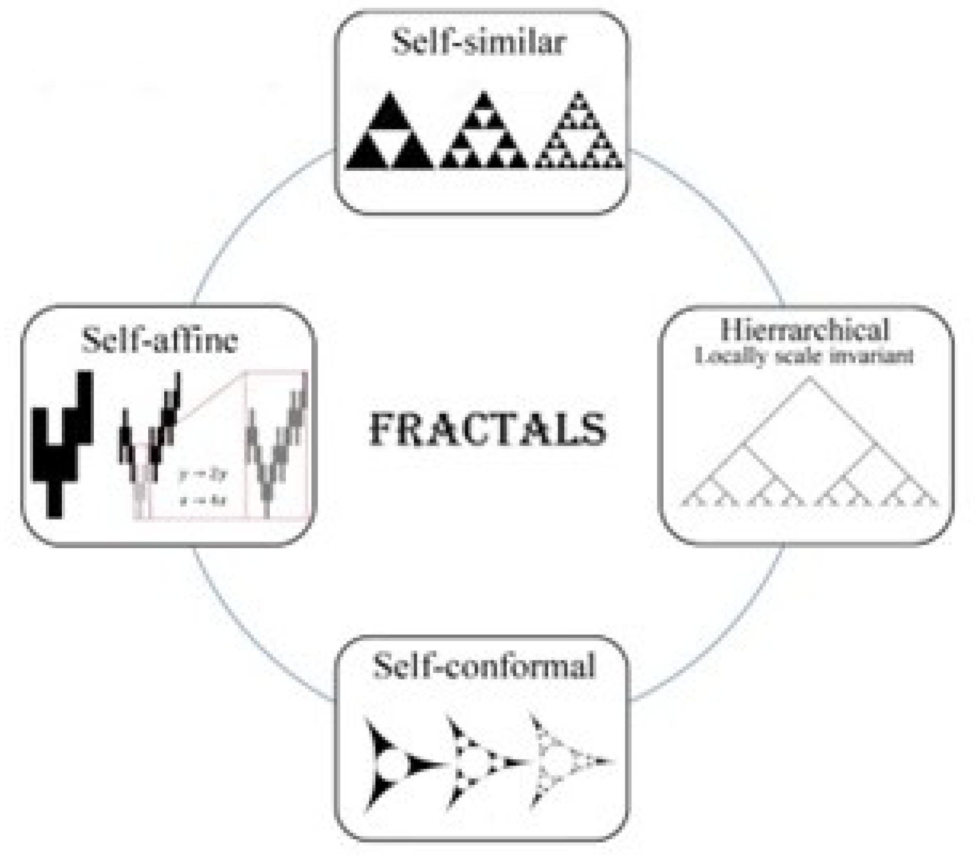
Figure 2.
Iterative construction of: (a) self-similar fractal and (b) hierarchical, locally self-similar fractal.
Figure 2.
Iterative construction of: (a) self-similar fractal and (b) hierarchical, locally self-similar fractal.
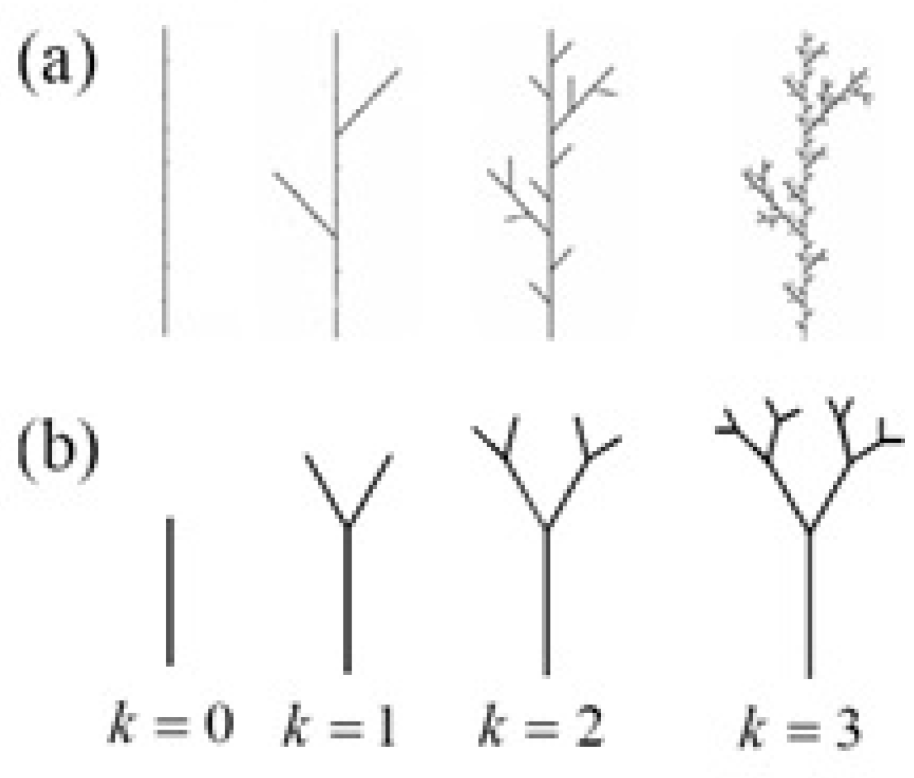
Figure 3.
The graph of Weierstrass function and its affine transformations.
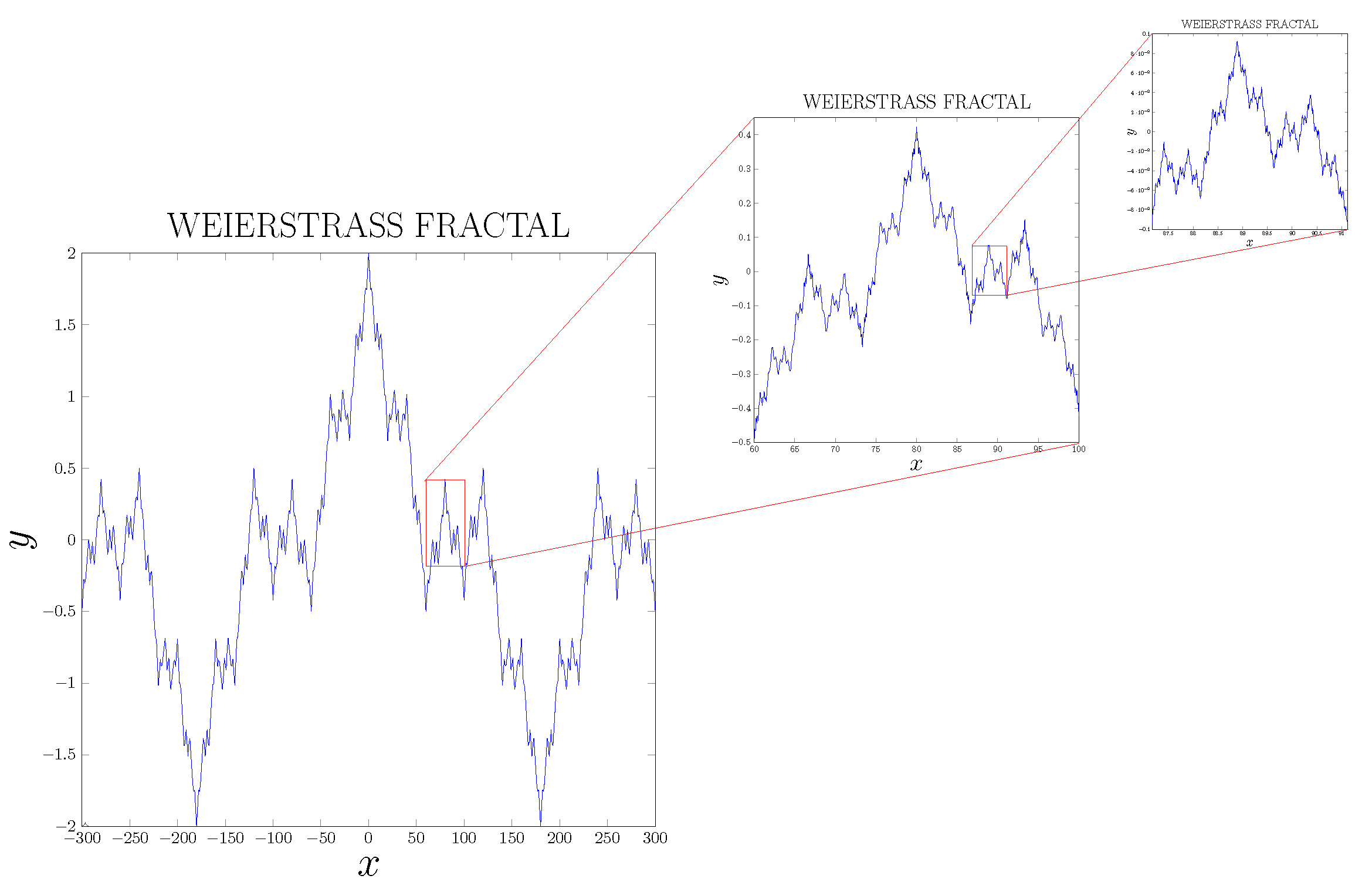
Figure 4.
Three steps of iterative construction of the middle third Cantor set.
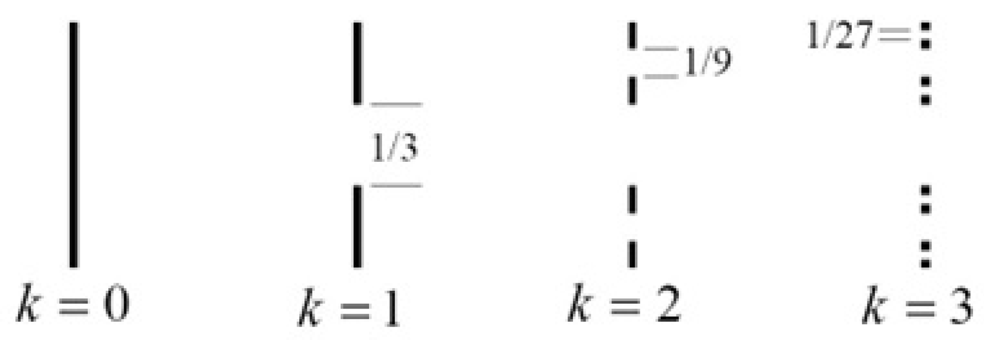
Figure 5.
Iterative construction of the space-filling curves: (a) Peano curve; (b) Hilbert curve; and (c) Sierpiński square snowflake.
Figure 5.
Iterative construction of the space-filling curves: (a) Peano curve; (b) Hilbert curve; and (c) Sierpiński square snowflake.
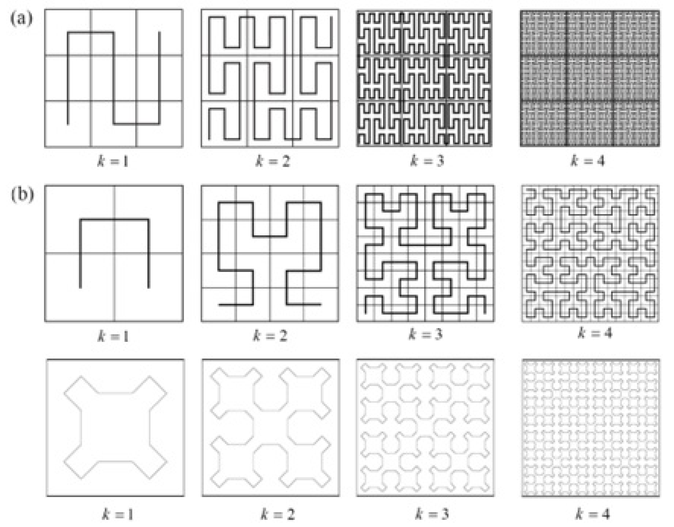
Figure 6.
(a), (b) Two ways to construct the Koch curve and (c) building the Koch snowflake
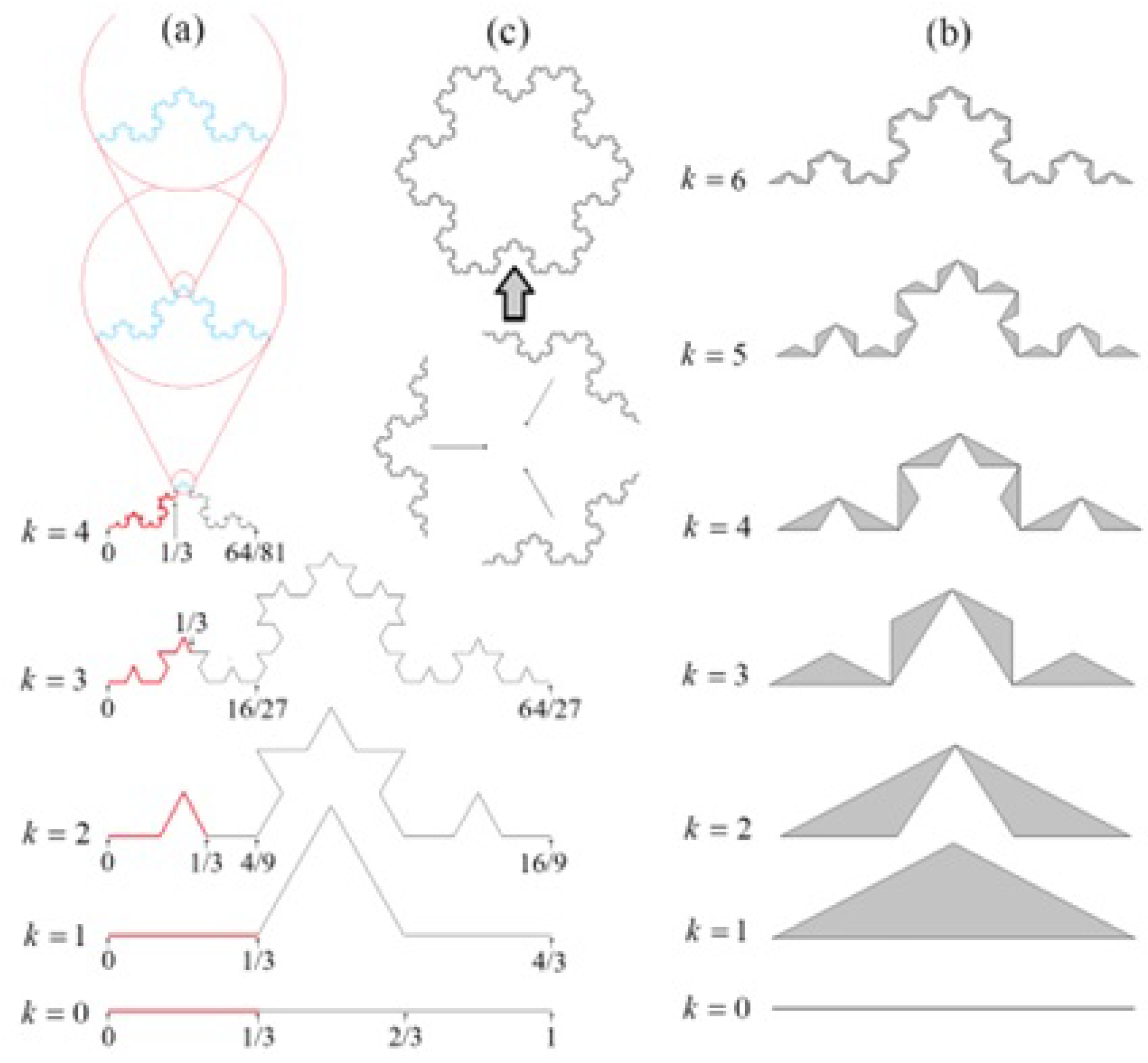
Figure 7.
Two ways to construct the Sierpinski triangle shape as the limits of the iterations of the pre-fractal: (a) Sierpinski gasket and (b) Sierpinski arrowhead curve.
Figure 7.
Two ways to construct the Sierpinski triangle shape as the limits of the iterations of the pre-fractal: (a) Sierpinski gasket and (b) Sierpinski arrowhead curve.
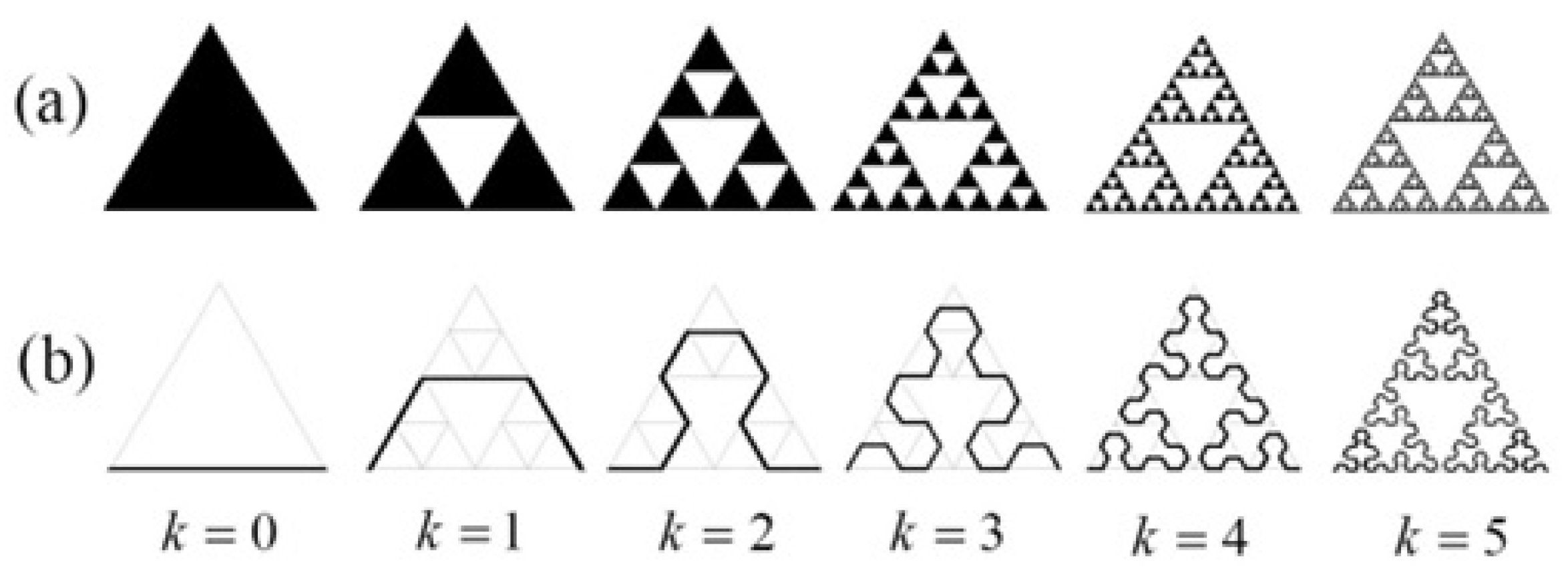
Figure 8.
Three first iterations of Sierpiński carpet and corresponding Sierpiński network.
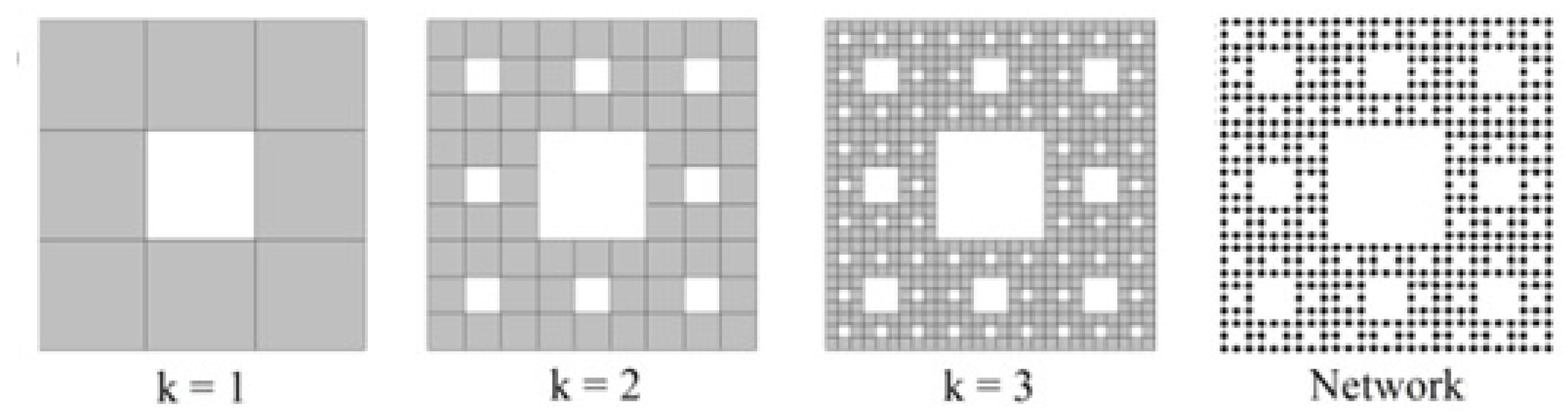
Figure 9.
Classification of objects with different kinds of scale symmetry.
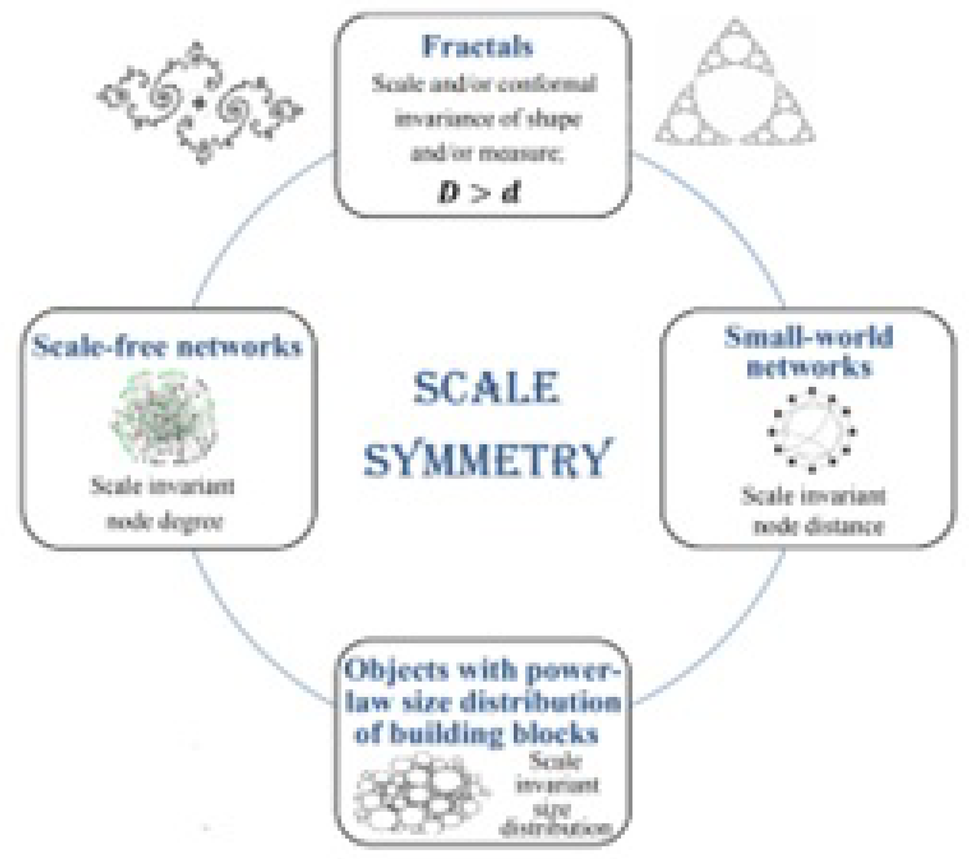
Figure 10.
Covering schemes associated with: (a) Hausdorff, (b) box-counting, and (c) Assouad measures.
Figure 10.
Covering schemes associated with: (a) Hausdorff, (b) box-counting, and (c) Assouad measures.
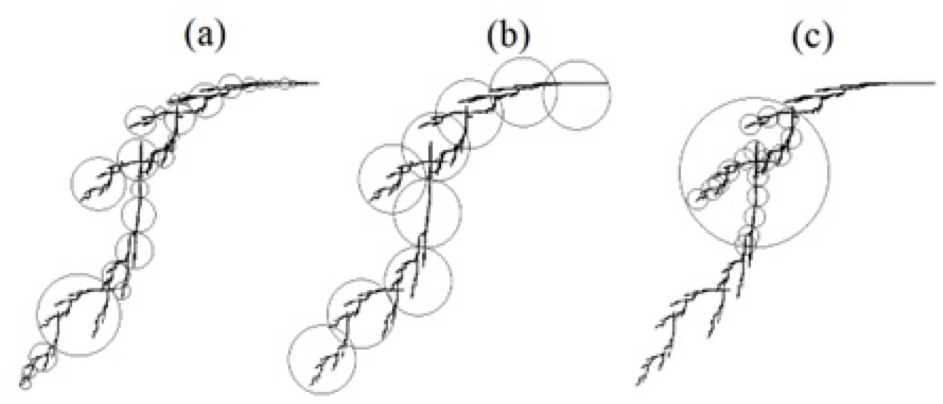
Figure 11.
Inherent features and key attributes of fractal patterns.
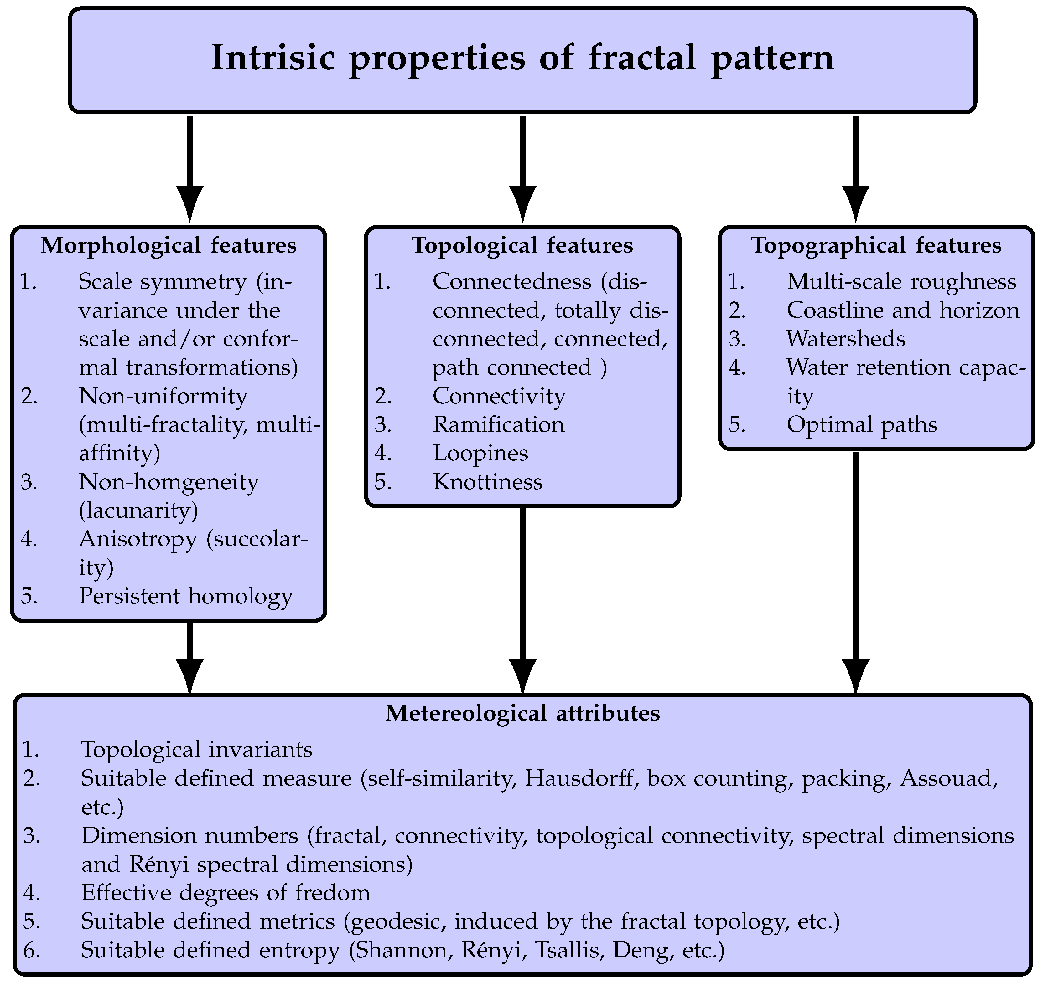
Figure 12.
Three first iterations of fractals having: (a) metric, (b) topological, and (c) combined origin.
Figure 12.
Three first iterations of fractals having: (a) metric, (b) topological, and (c) combined origin.
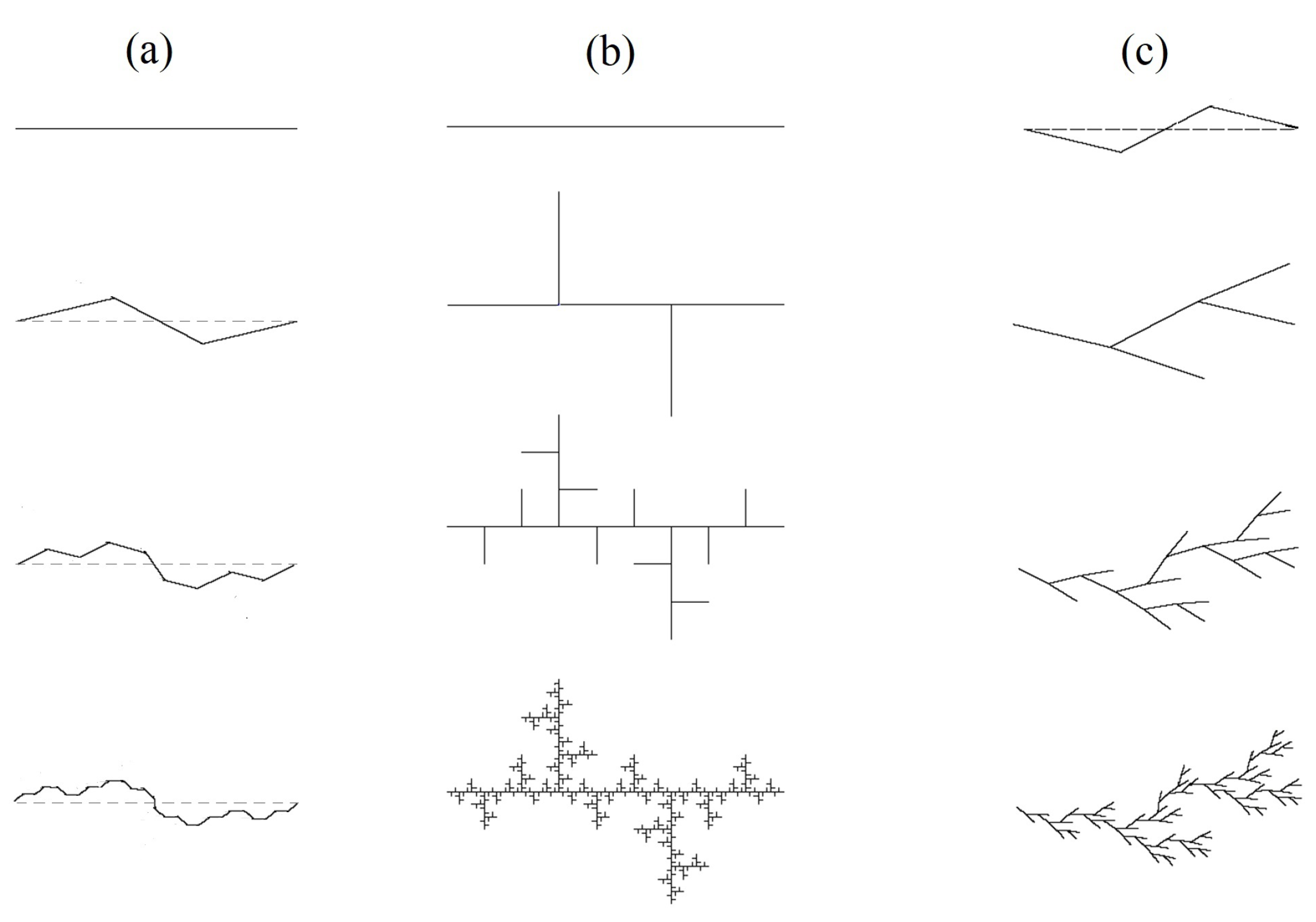
Figure 13.
Classification of scale invariant patterns from a topological viewpoint: (1) Euclidean pattern; (2) - (4) fractals of topological origin; (8) fractal of metric origin; and (5) – (7) fractals of combined origin. (1), (4), (5) - infinitely ramified; (2), (3), (6) – (8) – finitely ramified. Illustrations: Euclidean compliment of Menger sponge (1); fractal tree (2); Sierpiński gasket (3); Menger sponge (4); Julia-Mandelbrot set (5); diamond fractal (6); fractal leaf (7); fractal Koch-like curve (8).
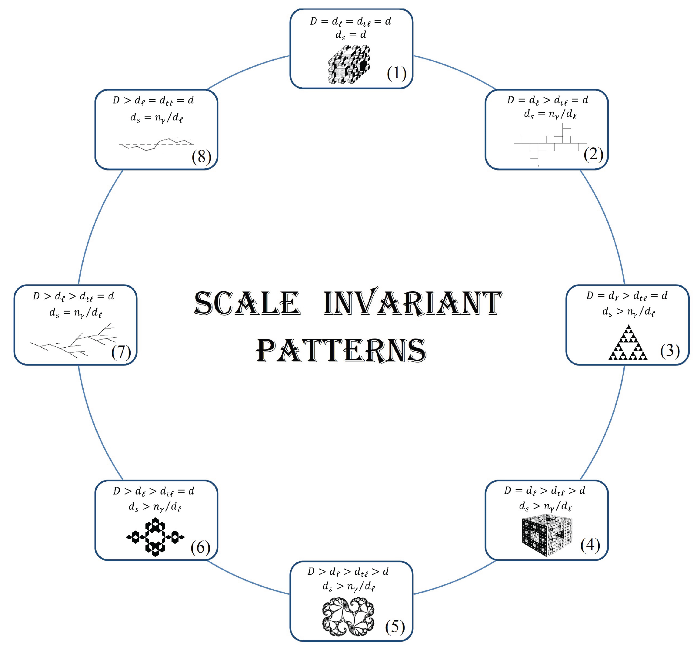

Table 1.
Some different definitions for fractal dimension.
| Dimension | Definition | Measure/Comments |
|---|---|---|
| Hausdorff-Besicovitch dimension | where U is any non-empty subset of n-dimensional Euclidean space, . Hausdorff meausre is , where , and diameter of U is | |
| Minkowski -Bouligand dimension | Let denotes the least number of balls in a covering of F by balls of radius . It is follows from the definition of that | |
| Minkowski dimension | is the parallel body to F: , for some , where n is the topological dimension | |
| Kolmogorov-Schirelman-Potjrajin | is the smallest number of balls of diameter less or equal to which are needed to cover fractal | |
| Mandelbrot-Schirelman-Kolmogorov | is the least number of balls of radius less than which are needed to cover fractal | |
| Upper box-counting dimension |
F is non-empty subset of . is any of the following:
|
|
| Lower box-counting dimension | ||
| box-counting dimension | ||
| upper modified box-counting dimension | If F can be decomposed into a countable number of pieces in such a way that the largest piece has a small a dimension as possible. | |
| Lower modified box-counting dimension | ||
| Packing dimension |
|
is a collection a disjoint balls of radius at most with center in F. Packing measures is: , where . |
| Assouad dimension | such that for all and | denote the covering balls (see for illustration Figure 10c). |
| Divider dimension (of Jordan curves) | -maximum number of points , on the curve C, in that order, such that , . |
Table 2.
Fractal attributes of some self-similar patterns.
| Figure | D | d | ||||||
|---|---|---|---|---|---|---|---|---|
| Cantor set C | 4 | 0 | 0 | See discussion in Ref. [110] | See discussion in Ref. [110] | See discussion in Ref. [110] | See discussion in Ref. [110] | |
| Cartesian product | See Ref. [4] | 1 | See discussion in Ref. [110] | See discussion in Ref. [110] | See discussion in Ref. [110] | See discussion in Ref. [110] | ||
| Cartesian tartan | See Ref. [111] | 1 | 0.387 | |||||
| Koch curve | 6 | 1 | 1 | 1 | 1 | 1 | 0 | |
| Sierpiński arrowhead curve | 7b | 1 | 1 | 1 | 0 | |||
| Koch curve | 12a | 1.99 | 1 | 1 | 1 | 1 | 1 | 0 |
| Tree | 12b | 1 | 1 | 1.188... | 1.741 | 0 | ||
| Leaf | 12c | 1 | 1 | 1.188... | 1.741 | 0 | ||
| Tree | 2a | 1 | 1 | 1.188... | 1.741 | 0 | ||
| Diamond fractal | 13(6) | 1 | 1 | 1.137 | 1.448 | 0.012 | ||
| Sierpiński gasket | 7a | 1 | 1 | 1.805 | 0.635 | |||
| Sierpiśki carpet | 8 | 1.806 | 1.979 | 0.384 | 0.635 | |||
| Sierpiśki cube | See Ref. [92] | 2 | 2.933 | 2.998 | 0.41 | |||
| Sierpiśki waveguide | See Ref. [2] | 2 | 2.806 | 2.98 | 0.596 | |||
| Menger sponge | 13(4) | 2 | 2.52 | 2.94 | 0.49 | |||
| Complement of Menger sponge | 13(1) | 3 | 3 | 3 | 3 | 3 | 3 | 2/3 |
| Percolation cluste in | See Ref. [81] | 91/94 | 1 | 1.6574 | 1.6617 | 1.317 | 2 | 0.053 |
| Percolation cluste in | See Ref. [97] | 2.52293 | 1 | 1.828 | 1.834 | 1.327 | 2.341 | 0.022 |
Disclaimer/Publisher’s Note: The statements, opinions and data contained in all publications are solely those of the individual author(s) and contributor(s) and not of MDPI and/or the editor(s). MDPI and/or the editor(s) disclaim responsibility for any injury to people or property resulting from any ideas, methods, instructions or products referred to in the content. |
© 2025 by the authors. Licensee MDPI, Basel, Switzerland. This article is an open access article distributed under the terms and conditions of the Creative Commons Attribution (CC BY) license (http://creativecommons.org/licenses/by/4.0/).
Copyright: This open access article is published under a Creative Commons CC BY 4.0 license, which permit the free download, distribution, and reuse, provided that the author and preprint are cited in any reuse.


