
Submitted:
10 July 2025
Posted:
11 July 2025
You are already at the latest version
Abstract
Energy conservation is one of the cornerstones of physics, associating with the invariance of physical laws over time. Any system with space-time translational symmetry must conserve momentum and energy according to Noether’s theorem. In this work, we explore how energy conservation manifests in a charged retarded field engine. The energy conservation asserts that the rate of change of total energy in the system i.e., mechanical and field energy is balanced by the energy flux through the surrounding surface. It ensures adherence to basic physics for operation inside physically realistic limitations. The energy equation has been analyzed order by order for a system of two arbitrary charged bodies. We used the expressions for the electric and magnetic fields obtained from the Taylor series expansion to account for the effects of retardation in the system. This analytical work concludes that the total energy in a charged field engine, including both mechanical and electromagnetic field energy, is indeed conserved up to fourth order, confirming that any changes in mechanical and field energy are balanced by the energy flux across the system’s boundary. As a consequence we demonstrate that the work done by the internal electromagnetic field in a retarded field engine is exactly balanced by the mechanical kinetic energy gained by the same engine.
Keywords:
electromagnetism
; retardation
; relativity
1. Introduction
Charged retarded systems represent a ground breaking approach to space propulsion, aimed at addressing the major limitations of traditional rocket fuel. Robertson et al. [1] reviewed the principal barriers slowing advancements in space propulsion technologies and highlights several theoretical ideas that, within the last twenty years, have evolved from speculative fiction into scientific theory. It is thus essential to explore various aspects of these systems, such as linear momentum and energy conservation, as all engines operate within the constraints of the laws of mechanics and the first law of thermodynamics: energy cannot be created or destroyed, only transformed.
This work discusses the retardation effects caused by the relativistic finite speed of signal propagation in a charged engine. As signals must propagate at a finite speed, it follows that an action and its corresponding reaction cannot occur simultaneously. Although retardation already exists in Maxwell’s equations relativity went even further to postulate that no object, message, signal (of any kind, including non-electromagnetic), or field can travel faster than the speed of light in a vacuum [2,3,4]. Griffiths and Heald [5] highlighted in their paper that Coulomb’s law and the Biot-Savart law are strictly valid only for determining electric and magnetic fields from static sources. To extend their applicability beyond the static domain, Jefimenko’s time-dependent generalizations [6] of these laws were formulated taking into account the retardation effect. In this case, momentum and energy are exchanged between the field and the material, enabling the relativistic engine effect. This result had already been observed and highlighted by several authors [7,8,9,10,11].
This process differs significantly from the transfer of momentum and energy between two material bodies which is the basis of standard transportation (a rocket ejects material to prorogate and a car must push the road to move forward). Relativistic effects indicate a novel type of motor, consisting not of two material components but of a combination of matter and an electromagnetic field. In [12] we provided a detailed analysis of the retardation effect and presents the conceptual framework and design principles underlying a charged relativistic motor. Recently, we [13] also investigated the interaction between charged bodies and magnetic currents generated by permanent magnetic materials, analyzing the potential implications for a charged relativistic engine utilizing a permanent magnet. Energy conservation has already been discussed in the case of uncharged relativistic engine [14], in which the energy transfer between the mechanical component of the relativistic engine and the electromagnetic field for a non charged engine. In this case the total electromagnetic energy utilized is six times the kinetic energy gained by the relativistic motor. Furthermore, previous research [15] has provided a mathematical proof that demonstrates that linear momentum is conserved in a retarded electric motor which is uncharged.
In the current work, we investigate a relativistic charged engine consisting of two subsystems of arbitrary geometry as in [12], with particular emphasis on the energy acquired by the system. We begin by analyzing the energy exchange between mechanical and electromagnetic components in the relativistic regime. Subsequently, we carry out a detailed examination of the engine’s energy dynamics by expanding the relevant field quantities as a power series in , where c denotes the speed of light in vacuum. This expansion systematically incorporates the effects of retardation. The total energy comprising mechanical energy, electromagnetic field energy, and energy flux via the Poynting vector is analyzed to verify the energy balance equation at each order. Specifically, we evaluate the contributions to the energy equation for and 4, demonstrating how retardation influences energy exchange and confirming that the energy balance is satisfied at each order within the accuracy of the expansion. Finally we demonstrate that the kinetic energy acquired by the engine exactly equals the amount of electromagnetic energy lost.
2. Energy Conservation
The conservation of energy in the general electromagnetic system is expressed by the following equation:
This equation reflects that any decrease (or increase) in the total energy within the system is accounted for by the energy carried away (or supplied) by the electromagnetic field through the system’s boundary. Here S denotes a closed surface enclosing the volume of interest, is a unit vector normal to the surface, represents a surface element.
Poynting’s vector is defined as:
Here, Fm−1 is the vacuum permittivity, (H/m) and m/s is the velocity of light in vacuum. The term represents the total electromagnetic power flux through the closed surface S. The field energy density is defined as:
and the derivative of the mechanical energy is the mechanical power given by:
where is the current density. Hence:
Or:
In what follows, we interpret equation (6) in terms of its role in governing energy conservation for a charged relativistic engine system.
2.1. Kinetic Energy
According to [12], the mechanical momentum associated with the time-dependent charged retarded field engine is expressed as:
or taking into account that: and defining as is customary that :
It is clear from the expression that the mechanical momentum is of the order of . The kinetic mechanical energy associated with this momentum is given by:
Where M is the mass of the relativistic engine and the engine velocity is defined as:
We notice that the expression for kinetic energy is of order , lower order corrections do not exist and higher order corrections are neglected.
3. Field Energy for Two Charged Sub-Systems
Consider two arbitrary charged sub-systems denoted system 1 and system 2 which are far apart such that their interaction is negligible. In this case, equation (6) is correct for each sub-system separately, that is:
Next we will put them closer together such that they may interact but without modifying the charge and the current densities of each of the subsystems. The total fields of the combined system are:
Since both the field energy equation (3) and Poynting’s vector equation (2) are quadratic in the fields, the following result is obtained:
The power invested in the combined system in bilinear in the current density and the electric field according to equation (4). This will lead to the following expression:
Subtracting from equation (6) the expressions given in equation (11) and equation (12):
taking into account equation (14)–equation (25) we arrive at:
4. Power Expansion in
Let us now expand equation (27) in power of , we introduce the notation to designate a term of order of the quantity G. Thus any quantity G may be written as the sum:
Specifically:
It follows from equation (25) that:
Also it follows from equation (17) that:
And finally from equation (21) it follows that:
In the subsections below we discuss equation (29) for different values of n starting from 0 up to 4. The analysis of the field contributions can now be carried out, considering each order in turn.
4.1. n=0
Let us look at equation (27) and study it for the zeroth order in :
4.1.1. Power
We shall start by calculating according to equation (30):
Equations (51) and (54) of [12] give a detailed expressions for the zeroth order term in the electric field expansion which is just the Coulomb field:
similarly:
where and define the relative position vectors:
By substituting equation (35) and equation (36) into equation equation (34), we obtain:
Applying the identities:
the expression in equation (38) can be simplified:
Or by changing the order of integration, in the form:
We next compute the individual integral terms to simplify the above equation:
Using Gauss theorem and continuity equation:
we obtain the following result:
The surface integral is performed over a surface encapsulating the volume of the volume integral. If the volume integral is performed over all space, the surface is at infinity. Provided that there are no currents at infinity i.e., ,
Similarly:
Substituting these identities in equation (41), we obtain:
Thus the power contains two contributions:
and
We now make a change of the integration variable in , thus and we obtain:
Similarly,
We now present the complete expression for the power:
Or equivalently:
4.1.2. Field Energy
Next we calculate field energy according to equation (31)
The magnetic field does not have terms which are lower than second order, we will use the null magnetic field expressions from Equation (58) of [12]:
Accordingly, the field energy takes the form:
Now solving separately the given integral:
Using the identity:
and taking into account that [3]:
in which is a three dimensional delta function. We obtain:
The first term on the right is a divergence. Thus, using Gauss theorem, its volume integral will become a surface integral, the second term contains a delta function. This means that there is no contribution to the volume integral from the delta term unless . Thus, equation (57) simplifies to:
Let us look at the surface integral and assume that the system is contained inside an infinite sphere, such that the surface integral is taken over a spherical surface of radius :
Here , in which is the solid angle. Also both , and . It follows that:
(see also Appendix of [14] for complete explanation of equation (62)). We conclude that simply:
Hence, the expression for the field energy becomes:
as ,
From equation (53) and equation (66), it is now clear that:
It follows that the power related to mechanical work equals minus the temporal rate of change of the field energy.
4.1.3. Poynting Vector
Finally we shall study the Poynting vector according to equation (32):
It is clear from equation (55), that:
as both and decrease as at infinity, it follows that their cross product decreases as , thus a surface integral over an infinite sphere will also vanish, which is what should be expected from equation (67) that balances the changes in the electromagnetic energy and mechanical power without any Poynting contribution. For , we conclude that the energy equation of order zero is indeed balanced as is expected.
4.2. n=1
Let us look at equation (27) and study it for the first order in :
4.2.1. Power
The first order expression for the power invested in mechanical work is given below:
According to equations (51) and (54) of [12], the first order term in the electric field expansion is:
Therefore,
4.2.2. Field Energy
4.2.3. Poynting Vector
Taking into account equation (55) and equation (72), the first-order expression for the Poynting vector is given by:
According to Equation (61) of [12], it follows that:
Hence:
Thus, for , we conclude that the energy equation of order one is indeed balanced in a trivial way. Equation (27) is satisfied in the sense that 0 = 0.
4.3. n=2
Let us look at equation (27) and study it for the second order in :
4.3.1. Power
The second-order expression for the power invested in mechanical work is given below:
We start by addressing the first integral in the above equation:
According to equations (51) and (54) of [12] the second-order term in the electric field expansion is:
Inserting this in the expression will result in:
We shall now change the integration variable as before, such that:
Let us look at the expression:
notice that:
From the continuity equation (43), and taking into account Gauss theorem and the vanishing of current densities on a far away encapsulating surface it follows that:
Thus, equation (85) takes the following form:
Upon substitution of equation (88) into equation (84), the resulting expression is:
Exchanging the indices 1 and 2, we obtain the second integral of equation (80):
Combining equation (89) and equation (90), we obtain the complete expression for the power:
Applying the product rule of derivatives we obtain:
Or:
Thus we obtained a power expression accurate to second-order.
4.3.2. Field Energy
We now proceed to calculate the field energy using equation (31) for :
As we already know that:
It follows that the field energy takes the simplified form:
This can be expressed as the sum of the following terms:
where
and,
We now compute the integral of each term separately:
The relevant field expressions are provided in [12] (and are previously mentioned in the current paper):
and
Substituting these field expressions into equation (101), we obtain:
Or in the form:
Let us look at the expression:
Taking into account equation (A.9):
Notice that:
And
Substituting these integral forms into equation (107), we obtain:
Next, we simplify the second integral appearing in equation (105):
As is known from [15]:
Subsequently, the required integral follows by a straightforward exchange of indices.
Thus:
Inserting the evaluated integrals into equation (105) yields:
Or:
We now focus on the second term to enable further simplification:
in the above we used equation (86) and equation (87). By substituting this result into equation (116), we arrive at:
Notice that the following terms would be zero considering equation (43), Gauss theorem, and the null current densities at the convergence radius :
Hence as the double integral in equation (118) decouples, it follows that:
Analogously, the second integral in the field energy expression also nullifies:
Next, we calculate the third integral to finalize the field energy equation, employing Equation (61) of [12]:
Similarly:
Hence,
Applying the following vector identity:
equation (124) can be rewritten as:
Similar to equation (45) it can be shown that:
Taking into account equation (64) and equation (127) it follows that:
Taking into account equation (B.4) we obtain:
the last equation sign is due to the fact that in the term containing the volume integrals decouple, and thus by equation (119) this term is null. Combining equation (129), equation (120) and equation (121), we obtain an expression for the second-order field energy:
4.3.3. Poynting Vector
Next, we shall study the Poynting vector according to equation (32) for :
by equation (95) we obtain the following resulting form of the Poynting vector:
The Poynting vector term, typically associated with radiation, contributes to the energy balance only through the surface integral over a closed surface enclosing the system. When this surface is taken to be spherical and located at a far distance , only the asymptotic forms of the electric and magnetic fields are relevant for evaluating the Poynting vector contribution. Accordingly, the expression for the Poynting flux on a far away sphere of radius is given by:
Following the approach used in the field energy analysis, the Poynting flux may likewise be represented as a sum of distinct terms, enabling the successive calculation of the corresponding integrals:
Such that:
and
According to Equation (57) of [12]:
Let us now write an asymptotic expression for the second order electric field:
By equation (119) we have:
Taking into account equation (D.5) we obtain:
the above expression decreases as . According to Equation (62) of [12]:
Let us now write an asymptotic expression for the second order magnetic field:
the above expression decreases as . From equation (142) and equation (144) it follows that the Poynting vector decays as , the associated surface integral over a large sphere with radius whose surface area grows as will decrease as , thus provided is large enough we consider this contribution to be negligible, that is:
Similarly:
Next, we compute the third integral:
According to Equation (55) of [12]:
Let us now write an asymptotic expression for the zeroth-order electric field:
As this vector is radially oriented and cross product of the above with any other vector must be perpendicular to the radial direction. It follows that the said cross product will have a zero scalar product with a radially oriented surface vector and thus:
similarly:
Thus by plugging equations (145, 146,150,151) into equation (134).
in which the equality sign is only correct to the current approximation. Hence there is no Poynting vector contribution to the energy balance. This is expected as the mechanical work equation (93) is balanced by the field energy loss equation (130) in second order terms of :
It is remarkable that no radiation losses need to be considered up to the second order approximation, this will have implication for the retarded field motor that we discuss in later sections of this paper.
4.4. n=3
Let us look at equation (27) and study it for the third order in :
4.4.1. Power
The third-order expression for the power invested in mechanical work is given below:
Equations (51) and (54) of [12] combine to yield the third-order terms in the electric field expansions:
We proceed to evaluate each integral individually.
Changing the order on integration we obtain:
Let us look at the expression:
in which we have changed the order of integrals and used the Einstein summation convention. Now by continuity:
hence:
Now:
However:
Thus:
Inserting equation (164) into equation (161) and using Gauss theorem we obtain:
Assuming lack of currents on a far away encapsulating surface, the above expression simplifies into:
Inserting equation (166) into equation (158), we obtain the form:
We now change the integration variable . Thus: , and also:
By switching the indices, we obtain the second integral:
Combining equation (168) and equation (169), we obtain:
The expression obtained thus represents the third-order mechanical power.
4.4.2. Field Energy
We now proceed to calculate the field energy using equation (31) for :
It is known from [12] (see also equation (95)) that:
Therefore, the field energy can be written as:
As the first and third-order electric field expression is given in equation (156), we shall now focus on the first integral in the above expression:
By separating the terms we obtain:
Using equation (39) we obtain:
since:
as is a function of and does not depend on , it follows that :
in which we used Gauss theorem and assumed as usual that there are no currents on the far away encapsulating surface. Thus it follows from equation (175) that:
We now evaluate the following integral independently:
this can also be written in the form:
Using Gauss theorem we can recast in the form:
Calculating the surface integral on a far away spherical surface of radius and assuming that all currents and charges are close to the origin of axis with distances much smaller than such that and , it follows that:
Thus equation (182) takes the form:
At this point we notice that up to rather small terms depends only on and not on , thus we may partition the double integral given in equation (179) in the form:
because (see equation (119)). Similarly:
By inserting the results of equation (185) and equation (186) into equation (173) we obtain a null result:
It follows remarkably that no electromagnetic energy can be stored at the third order of .
4.4.3. Poynting Vector
Next, we shall study the Poynting vector according to equation (32) for
by equation (172) the Poynting vector takes the form:
The Poynting flux on a far away sphere of radius is given by:
For ease of computation, we divide the Poynting flux expression into four independent integrals:
We begin by evaluating the first integral:
Let us now write an asymptotic expression for the third-order electric field given in equation (156):
Using equation (119), we obtain:
and an asymptotic expression for the second-order magnetic field:
Thus,
In the above we use the Einstein summation convention. Now the radial unit vector can be written in the cartesian coordinates in the form:
in which is the azimuthal angle, is the angle of latitude and are unit vector pointing in the direction of the Cartesian axes. Now:
As every non diagonal element of is calculated by integrating over a complete period, a term containing either or it follows that the non diagonal elements of this matrix vanish. It remains to calculate the diagonal elements:
Thus:
In which is Kronecker’s delta. Inserting equation (202) into equation (196) it follows that:
Analogously, the second integral of the Poynting flux takes the form:
We now proceed to evaluate the third integral:
As referenced earlier, we adopt the electric and magnetic field expressions provided by [12]:
and
Therefore:
In a similar manner:
Thus by inserting equation (203), equation (204), equation (208) and equation (209) into equation (191), we obtain the total Poynting flux contribution of the third order in :
This term is minus equation (170), that is minus the power invested by the electromagnetic field to do mechanical work to the third order in . It follows that in the third order no energy can be stored in the electromagnetic field and the energy equation is balanced between radiation and work. That is incoming radiation can cause charges to do work, or charges can radiate at the expense of their mechanical energy. However, if the currents in the two subsystems are orthogonal no radiation is radiated and no work is done.
4.5. n=4
Let us look at equation (27) and study it for the fourth order in :
4.5.1. Power
The fourth order expression for the power invested in mechanical work is given below:
According to equations (51) and (54) of [12], the fourth order term in the electric field expansion is:
Let us calculate both integrals of equation (212) one by one:
Changing the integration symbol from to , this takes the form of:
Exchanging the indices 1 and 2, we obtain the second integral of equation (212):
Adding the contributions, we finally obtain the fourth order power expression:
4.5.2. Poynting Vector
Next, we analyze the Poynting vector for using equation (32):
according to equation (172) the Poynting vector takes the following fourth order form:
Poynting flux on a far away sphere of radius is given by:
For each of the terms appearing in equation (219) we may write a Poynting flux, thus we obtain:
Let us now calculate the first term :
Calculating the electric field on a far away sphere, we may write equation (213) in the asymptotic form:
Taking into account equation (119), we obtain:
As current density integrals are related to charge density integrals through equation (D.5), it follows that:
The asymptotic expression for is given in equation (144). Using the asymptotic expressions, we are now in a position to calculate . Taking into account that radial components of either the electric or magnetic field do not contribute to the Poynting flux we obtain the following expression:
Inserting equation (202) into equation (226), it follows that:
Similarly, the second integral of the Poynting flux takes the form:
We now proceed to calculate:
The fourth order term of the magnetic field can be calculated using the asymptotic limit of Equation (61) of [12]:
Using the asymptotic form of the second order electric field given in equation (142), and recalling that the radial part of any field does not contribute to the Poynting flux we now obtain:
Using equation (202), we obtain:
In a Similar manner:
Subsequently, we calculate the fifth and sixth contributions appearing in equation (221):
The asymptotic form of the zeroth order electric field is given in equation (149) and has only a radial component hence it follows that:
Thus by inserting equation (228), equation (229), equation (233), equation (234), and equation (236) into equation (221), we obtain the total Poynting flux contribution of the fourth order in :
4.5.3. Field Energy
Now, the contribution of the field energy to the energy balance at fourth order is evaluated as follows:
Taking into account equation (172) the field energy simplifies as follows:
This can be separated into a sum of terms, such that for each term the integral is calculated separately:
Or in the form:
The following expression simplifies with the aid of equation (C.3) as follows:
Now let us evaluate the term:
this can also be written in the form:
Using Gauss theorem we can recast in the form:
Calculating the surface integral on a far away spherical surface of radius and assuming that all currents and charges are close to the origin of axis with distances much smaller than such that: and , we thus obtain:
Hence using equation (C.3) it follows that:
We now can write the triple volume integral given in equation (241) as a double volume integral:
Or more simply as:
Now for the term, the double volume integrals decouple, and following equation (119), we obtain:
Let us look at the term:
This can be written in the form:
Using Gauss theorem and the continuity equation (43) this can be written as:
Assuming no currents at far away surfaces this reduces to:
Plugging back into equation (250), we obtain:
In a similar fashion, the second integral of equation (239) is obtained by interchanging the indices:
Next we calculate using equation (82):
Which can be cast in the form:
To reduce the above triple volume integral into a double volume integral we notice that by using equation (C.3) it follows that:
Exchanging the 1 and 2 indices, we obtain:
Taking into account equation (B.6), it follows that:
The following integral can be computed using methods similar to those used in Appendix A such that:
Using equation (108) and equation (109), we obtain:
Thus:
Which can be slightly simplified:
The term decouples into a multiplication of two volume integrals and thus by equation (119) vanishes, thus we obtain:
The above can also be written in the following form:
Now:
In which we have used Gauss theorem and the continuity equation (43). Taking a far away encapsulating surface in which no currents are to be found, it follows that:
Similarly:
Plugging equation (269) and equation (270) into equation (268) we obtain the simplified expression:
To summarize the electric part of the fourth order electromagnetic energy can be written in terms of the temporal derivatives of charge and current densities in the form:
We remind the reader that is the maximal radius for which the Taylor series expansion is applicable. Ir remains to calculate the magnetic terms contributions, a task which we shall now attend to. Set:
Now by Equation (61) of [12]:
Plugging equation (274) and equation (275) into equation (273) it follows that:
By a well known vector identity:
we may write equation (276) in the form:
Notice that:
In the above, we have used the Gauss theorem, assumed that there is no current density on far away surfaces, and used the continuity equation (43). Similarly:
Plugging equation (110), equation (279) and equation (280) into equation (278), we arrive at the expression:
Taking into account equation (C.3), the above expression reduces to:
The term containing decouple into a multiplication of two volume integrals. However, by equation (119) and due to the fact that we assume no current density on the far away encapsulating surface it follows that: and . We thus obtain a simplified form of equation (282):
By analogy:
Summing up equation (283) and equation (284) we arrive at the fourth order contribution to the magnetic field energy in terms of a double volume integral:
Hence, adding the fourth order electric field energy given in equation (272) with the fourth order magnetic field energy contribution given in equation (285) we arrive at the total field fourth order energy:
This expression can be partitioned into volume contribution and surface contribution, in which the later type of contributions involves designating the maximal distance to which our expansion is applicable and thus also the radius of the sphere in which our energy calculations are performed. Thus:
It can be shown after a few lines of calculations that:
in which is the mechanical work done by the system and is given in equation (217). For the surface term we may only write:
in which is the Poynting Flux given in equation (237). Although both sides of equation (289) contain the same type of expressions the numerical factor are only of the same order of magnitude not identical, this is probably due to the crude approximations used in Section 4.5.2 and in the appendices. Notice, however, that this will not change the final results of the current paper.
5. Discussion
In order to verify the validity of the energy balance equation at various orders of approximation, we systematically evaluate the mechanical work, field energy, and Poynting vector contributions corresponding to successive terms in the Taylor expansion of the electromagnetic fields. Each term, labeled by the index n, represents a distinct order in the expansion and contributes differently to the total energy dynamics of the system. Below, we summarize the outcome of this analysis for through , highlighting the nature of energy exchange and the role of radiation at each order. For , the zeroth order energy equation is found to be satisfied. Mechanical work performed on or by the system leads to a corresponding increase or decrease in the field energy, as expected in the absence of any contribution from the Poynting vector. For , we find that the first-order energy equation is trivially satisfied, that is, it reduces to the identity under the condition that the mechanical work, field energy, and Poynting contribution all vanish individually. A vanishing mechanical work implies that, to first order in , no mechanical energy is either supplied to or extracted from the relativistic engine. Furthermore, the first-order terms in the expansion do not contribute to either the field energy or the Poynting vector associated with the engine. In other words, at first order, the electromagnetic fields neither store energy nor transport it through radiation or absorption, indicating the absence of any real energy exchange. For , We conclude that the second-order energy equation is indeed balanced: the power associated with mechanical work equals the negative time derivative of the field energy, as expected in the absence of any Poynting contribution. In the case , the absence of field energy implies that the electromagnetic field cannot store energy, leading to an energy balance strictly between radiation and mechanical work. Thus, incident radiation has the potential to drive charged particles to perform work. However, when the currents in the two subsystems are orthogonal, radiation is not emitted, and consequently, no work is done. It is also important to note that, if not properly configured, a relativistic motor may emit radiation. This behavior has been demonstrated in earlier studies involving uncharged relativistic motors [16]. For , We conclude that the fourth-order energy balance holds. At this order, both the electric and magnetic field energies are influenced by the mechanical work. At the order of , the structure of our series expansion limits our ability to evaluate the radiation flux at infinity. Instead, we must restrict our analysis to the radiation flux through a spherical surface of radius , beyond which the validity of our approximation breaks down. We also notice that for terms dependent on the approximation we use here is not sufficient to exactly balance the terms of the energy change and the Poynting flux, for which a better approximation is required.
Our motivation for this study is to understand the energy exchange in a relativistic motor, however, for this motor one needs to consider only first order derivative of the charge density. On the other hand terms in the energy equation depend on higher derivatives, this problem will be resolved in the next section.
6. The source of the Charged Retarded Field Engine Energy
So far our discussion was quite general, we have calculated the energy balance terms for various orders of up to . We did not pay specific attention to the characteristics of the relativistic engine which we shall consider now. Suppose we have two static charge distributions consisting of a retarded field engine, and suppose one induces a time dependent change in one of the charge distributions generating momentum according to equation (8) after which the charge distribution becomes static again as in Figure 1.
Notice, that at this point we have two static charge distributions in the engine’s frame but not in the laboratory frame. In the laboratory frame the two subsystems connected with the engine are now moving with velocity (see equation (10)) which is the velocity of the engine. The engine has gained a kinetic energy given by equation (9), we shall now inquire regarding the source of this energy.
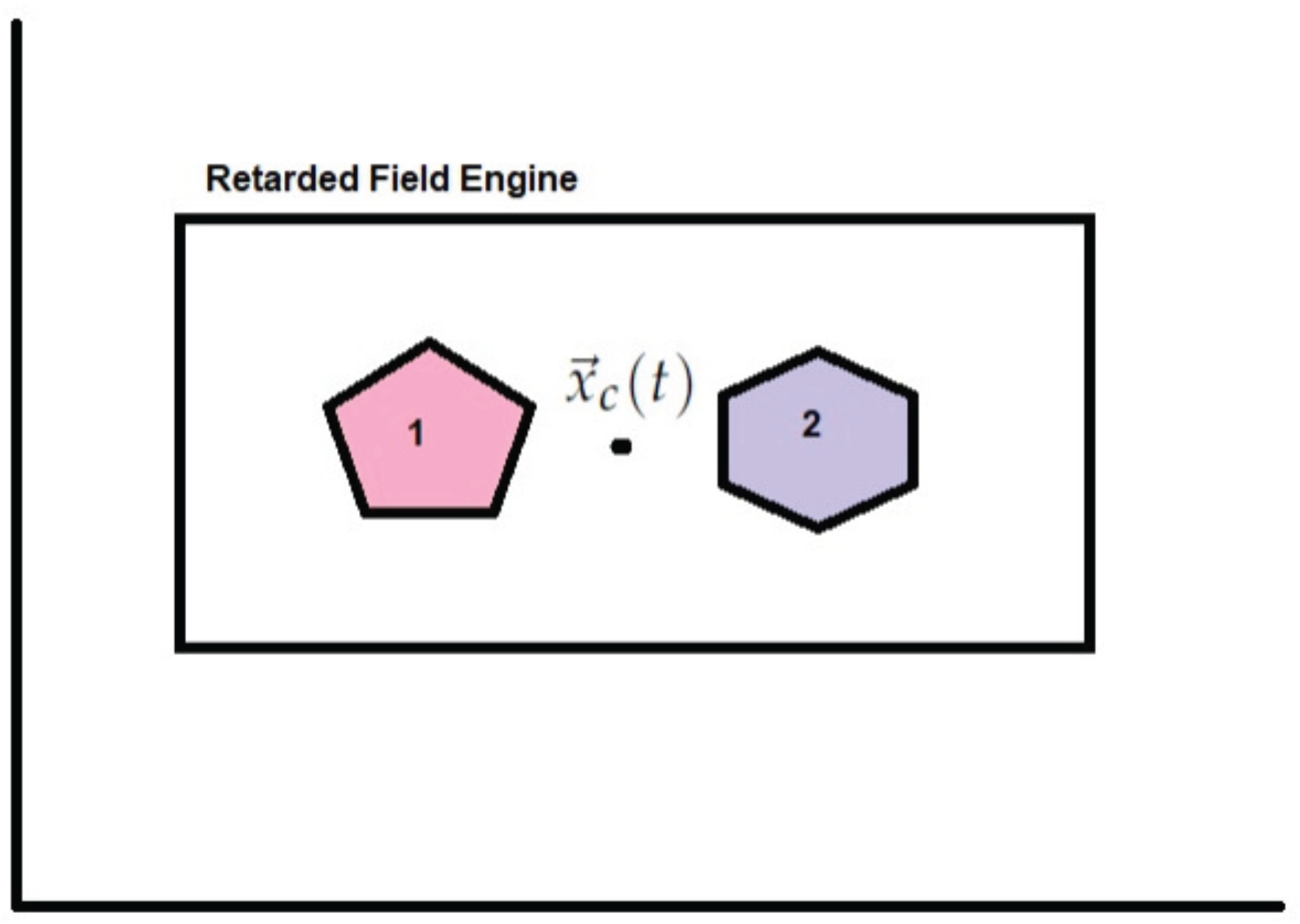
Let be the location vector of a point in the laboratory (inertial) frame, and let be the location of the engine in that frame as in Figure 2.
It follows that the location of the same point with respect to the engine is:
And also that:
The charge density can be expressed in either the laboratory (inertial) frame or in the engine frame. In the first case it is designated by and in the second by , those two functions are related as follows:
In the case that the charge distribution is "static" in the engine frame this reduces to:
Similarly the partial temporal derivative can be calculated as follows:
And for the case the charge density is "static" in the engine frame this reduces to:
Taking into account the continuity equation (43) we notice that although no current densities were initially assumed in the system, it now follows that from the laboratory point of view the engine now carries current density of the form:
We are now at a position to calculate the work done by the internal electric field in such a system. This is done by using equation (93) which describes the time derivative of this work. We remind the reader that we have shown this work to be exactly equal to the amount of energy change in the electromagnetic field (see equation (130)). Thus:
This can be written in the form:
Taking into account equation (295) and equation (296) it follows that:
Notice that:
Using Gauss theorem and equation (86) this can be written in the form:
in which we assume as usual that there is no charge on a far encapsulating surface. Similarly:
Plugging equation (301) and equation (302) into equation (299) it follows that:
The linear momentum is given by equation (8) and the kinetic energy was defined in equation (9). Hence the work done by the retarded electromagnetic field is converted into the kinetic energy of the retarded field engine. We have used a expression for the work but since is proportional to it turns to be proportional to as previously discussed thus resolving the dilemma stated in the end of the previous section.
7. Conclusions
A relativistic engine is not a self-sustaining device nor is a perpetuum mobile, it requires an input of energy to function. This energy is drawn from the electromagnetic field, reducing its energy in the process. In this study, we explore the validity of energy conservation in relation to a charged retarded engine. This research focuses on how energy is conserved in charged retarded systems, proposing an exciting new way to power spacecraft. By using electromagnetic fields instead of traditional rocket fuel, this technology could help spaceships travel faster and farther while using much less energy.
Author Contributions
Conceptualization, A.Y.; methodology, A.Y. and P.S.; formal analysis, A. Y. and P.S.; investigation, A. Y. and P.S.; writing—original draft preparation, P.S.; writing—review and editing A.Y. and P. S.; supervision, A.Y.; project administration, A.Y. All authors have read and agreed to the published version of the manuscript.
Funding
This research received no external funding.
Institutional Review Board Statement
Not applicable.
Informed Consent Statement
Not applicable.
Data Availability Statement
The original contributions presented in the study are included in the article, further inquiries can be directed to the corresponding author.
Conflicts of Interest
The authors declare no conflicts of interest.
Appendix A. Simplification of Certain Integrals
We know that: , as is constant with respect to the integration it follows that: , so
Using spherical coordinates: :
we may write equation (A.1) in the form:
We now recall the definitions:
Using the above equation for we obtain:
Let us choose the z axis in our spherical coordinates to be in the direction.
and let us expand:
since . We now introduce the dimensionless variable: . Thus equation (A.5) takes the form:
Taking into account the solid angle expression given in equation (A.2) we finally obtain:
is a radius of sphere whose surface is presumably far away from the charged systems and defines the limit in with the Taylor series expansion is applicable.
Appendix B.
where
Let ,
Thus:
Appendix C.
As in Appendix A:
in which we have replaced the integration variable with the integration variable , and we use spherical coordinates as in equation (A.2). Again we use the dimensionless variable , and obtain:
Now taking into account equation (B.4) it follows that:
Appendix D.
Let us calculate a volume integral of a current density component:
in which is Kronecker’s delta and Einstein summation convention is assumed regarding repeated indices. Thus:
where in the last equation sign we have switched to vector notation. Taking into account Gauss theorem and the continuity equation (43), it follows that:
Assuming no currents on the (far away) encapsulating surface the surface integral vanishes. Adopting vector notation we have:
in the above is the system (or subsystem) electric dipole moment. It follows that:
References
- Robertson, G.A.; Murad, P.; Davis, E. New frontiers in space propulsion sciences. Energy Conversion and Management 2008, 49, 436–452. [Google Scholar] [CrossRef]
- Einstein, A. On the electrodynamics of moving bodies 1905.
- Jackson, J.D. Classical electrodynamics, 3rd ed. ed.; Wiley: New York, NY, 1999.
- Feynman, R.P.; Leighton, R.B.; Sands, M. The Feynman lectures on physics, Vol. I: The new millennium edition: mainly mechanics, radiation, and heat; Vol. 1, Basic books: New York,New York,USA, 2011.
- Griffiths, D.J.; Heald, M.A. Time-dependent generalizations of the Biot–Savart and Coulomb laws. American Journal of Physics 1991, 59, 111–117. [Google Scholar] [CrossRef]
- Jefimenko, O. Electricity and Magnetism 2nd edn; Electret Scientific: Star City, WV:, 1989. [Google Scholar]
- Breitenberger, E. Magnetic interaction between charged particles. American Journal of Physics 1968, 36, 505–515. [Google Scholar] [CrossRef]
- Scanio, J. Conservation of momentum in electrodynamics - an example. American Journal of Physics 1975, 43, 258–260. [Google Scholar] [CrossRef]
- Portis, A. Electromagnetic Fields, Source and Media; John Wiley & Sons Inc: New-York, NY, USA, 1978. [Google Scholar]
- Jefimenko, O. A Relativistic Paradox Seemingly Violating Conservation of Momentum in Electromagnetic Systems. Eur. J. Phys. 1999, 20, 39. [Google Scholar] [CrossRef]
- Jefimenko, O. Cuasality, Electromagnetic Induction and Gravitation 2nd edn; Electret Scientific: Star City, WV:, 2000. [Google Scholar]
- Rajput, S.; Yahalom, A. Newton’s Third Law in the Framework of Special Relativity for Charged Bodies. Symmetry 2021, 13, 1250. [Google Scholar] [CrossRef]
- Sharma, P.; Yahalom, A. A Charged Relativistic Engine Based on a Permanent Magnet. Applied Sciences 2024, 14, 11764. [Google Scholar] [CrossRef]
- Rajput, S.; Yahalom, A.; Qin, H. Lorentz symmetry group, retardation and energy transformations in a relativistic engine. Symmetry 2021, 13, 420. [Google Scholar] [CrossRef]
- Tuval, M.; Yahalom, A. Momentum conservation in a relativistic engine. The European Physical Journal Plus 2016, 131, 1–12. [Google Scholar] [CrossRef]
- Rajput, S.; Yahalom, A. Material Engineering and Design of a Relativistic Engine: How to Avoid Radiation Losses. In Proceedings of the Advanced Engineering Forum. Trans Tech Publ, 2020, Vol. 36, pp. 126–131.
Figure 1.
A change is introduced momentarily to after which it becomes static.
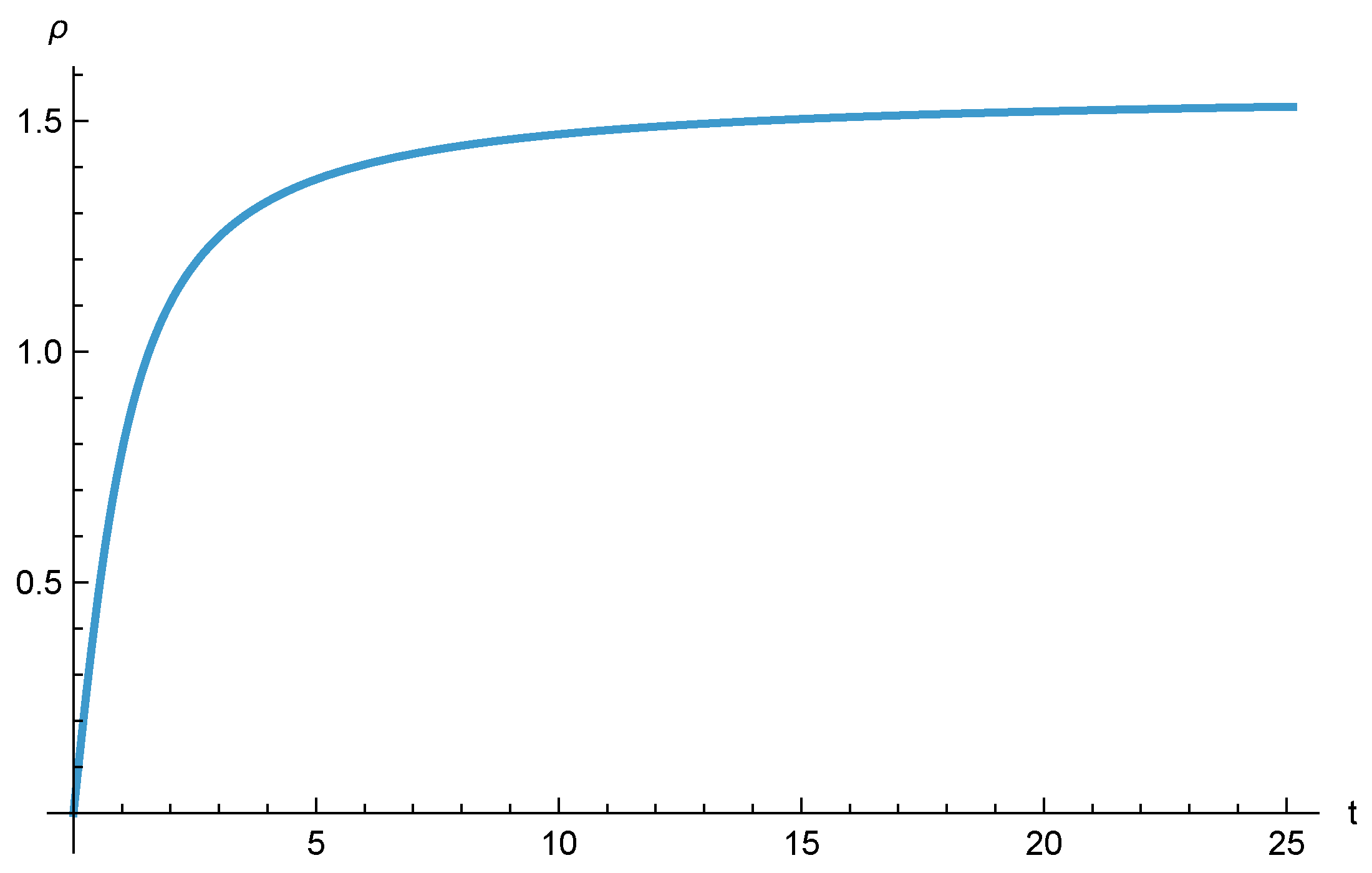
Figure 2.
The Retarded field engine comprised of charged subsystems 1 and 2, the engine is located at with respect to the inertial system.
Figure 2.
The Retarded field engine comprised of charged subsystems 1 and 2, the engine is located at with respect to the inertial system.
Disclaimer/Publisher’s Note: The statements, opinions and data contained in all publications are solely those of the individual author(s) and contributor(s) and not of MDPI and/or the editor(s). MDPI and/or the editor(s) disclaim responsibility for any injury to people or property resulting from any ideas, methods, instructions or products referred to in the content. |
© 2025 by the authors. Licensee MDPI, Basel, Switzerland. This article is an open access article distributed under the terms and conditions of the Creative Commons Attribution (CC BY) license (http://creativecommons.org/licenses/by/4.0/).
Copyright: This open access article is published under a Creative Commons CC BY 4.0 license, which permit the free download, distribution, and reuse, provided that the author and preprint are cited in any reuse.


