
Submitted:
07 August 2025
Posted:
08 August 2025
You are already at the latest version
Abstract
Addressing the potential conflicts between momentum conservation laws and retardation requires a comprehensive understanding of both principles within the context of specific physical systems and theoretical frameworks. Indeed it was claimed that a retarded engine is impossible due to the lack of linear momentum conservation. The purpose of this work is to settle this issue by demonstrating that linear momentum is indeed conserved for a charged retarded field engine. Earlier research has already introduced the concept of a charged retarded engine. The system gains mechanical momentum and energy when it is subjected to a total force for a certain amount of time. If retardation is taken into account a total force is present even if no external force affects the system, thus momentum seems to appear from nowhere violating the law of momentum conservation. However, momentum is indeed conserved as the present work demonstrates. We present a mathematical proof that the momentum is conserved in a time dependent electromagnetic retarded motor. The expression of field momentum comes out to be equal and opposite to the mechanical momentum gained by the material system as obtained in [1]. This calculation of charged retarded engine is an extension work of papers published earlier [2,3] which explored a non-charged retarded engine. We prove that the total momentum in a retarded motor including both material and electromagnetic linear momentum is indeed conserved as dictated by Noether’s theorem. This is a consequence of the non linearity of the electromagnetic linear momentum which is proportional to the integral of the vector multiplication of the electric and magnetic fields. The problem solved is relevant because it demonstrates that the charged retarded f ield engine does not violate any known physical laws and thus can serve for (space) transportation. The scientific novelty of the solution obtained is in demonstrating that a charged retarded field engine conserves linear momentum. Thus the momentum obtained by the field is equal and opposite to the linear mechanical momentum obtained by the engine.
Keywords:
Newton’s third law
; electromagnetism
; retardation
; nonlinearity of the electromagnetic linear momentum
; conservation of momentum
1. Introduction
The foundation of modern science was established by Newton’s laws of motion [4,5]. These rules explain how motion reacts to acting forces and how those forces relate to one another [4,5]. In his 1687 publication Philosophiae Naturalis Principia Mathematica, Isaac Newton formulated three fundamental rules [4,5,6]. Here we deal with the third law only which state: When a body applies force to another, the second body reciprocally applies a force of equal magnitude but opposite direction onto the first body. As per Newton’s third law, in a system unaffected by external forces, the total force sum is zero [4]. This principle has undergone numerous experimental validations and stands as a fundamental pillar of physics [5,6]. However, due to the finite speed of signal propagation, it is evident from the theory of relativity (but also prior to that from Maxwell’s equations of the fields) that an action and its reaction cannot be formed simultaneously [7]. In accordance with the theory of relativity, it is postulated that no object, message, signal (regardless of its nature, even if non-electromagnetic), or field can exceed the speed of light in a vacuum [8,9]. As a result, the forces cannot add up to zero [8]. However, as Griffiths & Heald [10] pointed out, retardation can be disregarded in the quasi-static approximation.
The majority of contemporary engines operate on the principle that two material components acquire momentum, one of which is equal to and opposite from the momentum acquired by the other (for example a rocket that propels itself by ejecting matter) [5]. Nevertheless, retardation effects indicate a novel motor design where the system doesn’t consist of two material bodies, but rather a material body in conjunction with a field [1]. In [1] we thoroughly elucidated the concept of a retarded engine, delving into its significance for space exploration [11,12]. A retarded engine is a type of propulsion system where the motion of the center of mass is achieved through the interaction between its internal components, which may either move relative to one another or remain fixed within a rigid structure [1]. The focus is primarily on the movement of the center of mass, which can occur in all directions, including vertical motion [1]. Unlike traditional engines, a retarded engine doesn’t have moving mechanical parts or rely on conventional fuel, thereby eliminating the need for fuel combustion and reducing carbon emissions [1]. It operates by harnessing electromagnetic energy, such as from solar panels, making it especially advantageous for space travel, where large amounts of fuel storage are typically required [1]. This approach offers a cleaner, more efficient way to power spacecraft [12].
Yet some scholars claim that such device cannot exist as it does not respect conservation of linear momentum, it is especially those scholars for which the current paper is written [1]. In a nutshell, linear momentum is conserved in such a device if one takes both mechanical linear momentum and electromagnetic linear momentum into account [1].
Griffiths and Heald [13] noted that the laws of Coulomb and Biot-Savart govern the configurations of electric and magnetic fields exclusively for stationary sources. Time-dependent extensions of these laws, as outlined by [14], were employed to explore the validity of Coulomb and Biot-Savart formulas beyond static conditions.
In an earlier work, the author addressed the force between two current-carrying coils [2] using Jefimenko’s [7,14] equation. Later on, this was extended to encompass the relationship between a permanent magnet and a current-carrying loop [15]. The earlier calculations have showed the expressions for mechanical momentum and field momentum when dealing with macroscopically neutral bodies and verified the conservation of momentum [3]. However, in the case of charged retarded engine, momentum conservation was still a question [3]. Energy conservation in an uncharged retarded motor was also discussed [16].
The case of a charged retarded motor was discussed in [1] but without discussing in detail the problem of momentum conservation.
In the present work, we have calculated the field’s momentum when electromagnetic fields are time dependent and compared with the mechanical momentum of the same system which comprises of two arbitrary charged bodies [1]. The main result of this work is that the field momentum for a two charged body system is equal and opposite to the mechanical momentum gained by the material components [1]. This result is not new, as it was already pointed out by a few authors [17,18,19,20,21]. In particular Feynman [9] describes two orthogonally moving charges, apparently contradicting Newton’s third law, as the forces that the charges induce do not cancel (last part of 26-2); this is resolved in 27-6 in which it is noticed that the momentum gained by the two-charge system is lost to the field. However, here we derive a general expression for field momentum that is applicable to any charge density and current density and not just point particles and prove mathematically that the total linear momentum of matter and field is indeed conserved, we underline that previous papers on the subject do not cover our results [1]. This is a consequence of the non linearity of the electromagnetic linear momentum which is proportional to the integral of the vector multiplication of the electric and magnetic fields [7]. This result can be applied also to quantum systems [22].
The scientific novelty of the solution obtained is in demonstrating that a charged retarded field engine conserves linear momentum. Thus the momentum obtained by the field is equal and opposite to the linear mechanical momentum obtained by the engine. Showing this is the purpose of our scientific research. Detailed structure of the article including the presentation of solved problems in the following sections are as follows: First we define the general formalism of electromagnetism in four dimensional notation, then we partition space and time and obtain the momentum conservation equation in standard notation. Then we partition the system to two subsystem and calculate the relation between the mechanical momentum and the field momentum which result from the interaction of the two subsystems. In the next section we show by explicit calculation up to the relevant order that the interaction field momentum is indeed equal in magnitude and opposite in sign to the mechanical momentum thus the sum of the two is always null. This is followed by a concluding section.
2. Electromagnetic Field Momentum
The field equations of electromagnetism can be written in a four dimensional form (CGS units) [7]:
where Greek letters take the values: , is the field tensor and is the four current. The Einstein summation convention is implied and so is the standard notation of lowering and raising indices. The above equation can be derived from a four dimensional action principle:
in the above is the four potential. The field tensor and four potential are related according to:
The above action is symmetric with respect to the Poincaré group and in particular symmetric to coordinate translation which leads to conserved currents given in terms of the symmetric energy momentum tensor:
in which is the Lorentz metric. Taking only the spatial Noether current we obtain the field linear momentum:
Latin indices take the values: . If the matter action is also considered one must add to the matter Noether current which corresponds to the matter linear momentum. In what follows we discuss the conservation of linear momentum which corresponds to the equation (MKS units) in terms of the standard formalism for which space and time are separated:
In the above, represents the i-th component of the mechanical momentum within the system, while denotes the i-th component of the field momentum. stands for the Maxwell stress tensor. S denotes a closed surface that encloses the volume where the system is situated, with representing a unit vector perpendicular to the surface. Additionally, the notation assumes Einstein’s summation convention. , Maxwell stress tensor can be calculated from the electromagnetic fields as follows:
Here, Fm−1 is the vacuum permittivity, c is the velocity of light in vacuum and is Kronecker’s delta.
The field linear momentum is defined to be:
3. System Partition
Suppose we have a given distribution of charge and current densities denoted by and respectively, those are known function of space and time. It is well known that in such a case we will have by virtue of Maxwell equations the following expressions for the electric and magnetic field evaluated at the location at time t [7,14]:
And:
Here N m2/C2, (H/m) (or Newtons per ampere squared) is the vacuum magnetic permeability (we use MKS units), charge and current densities are evaluated at .
Let us partition the above system arbitrarily into two subsystems such that:
Here again the charge densities and are assumed to be given functions of space and time, the same holds for and . From the linearity of Equation (9) and Equation (10) it follows that:
Such that:
and:
It is obvious that the electric field and magnetic field solve Maxwell equations for the charge density and current density and hence all theorems related to solutions of those equations hold. In particular Equation (6) holds, taking the form:
Similarly it is obvious that the electric field and magnetic field solve Maxwell equations for the charge density and current density and hence all theorems related to solutions of those equations hold. In particular Equation (6) holds, taking the form:
We will assume that the mechanical momentum of each subsystem is insignificant.
As both Equation (8) governing field momenta and Equation (7) describing the Maxwell stress tensor are quadratic in the fields, the following outcome is attained:
Subtracting the expressions given in Equation (18) and Equation (19) from Equation (6):
now with the help of Equation (20) and Equation (21) we obtain:
Next, we use the assumption that the mechanical momentum produced within each subsystem is insignificant compared to the mechanical momentum generated in one subsystem as a result of the fields produced in the other subsystem, and vice versa. Consequently, the self-generated mechanical momenta are negligible, yielding:
It is well known that analytic expressions for both the electric and magnetic fields [7,14] (see also Equation (9) and Equation (10) above) contain terms which reduce as and terms which reduce as , the later are proportion to at least (and higher powers of ). Now the surface area grows as , thus the surface integral will converge at large distances to for any square of terms. For mixed terms of the and type it will converge at large distances to . Thus at infinity we will be left with a multiplication of terms which must be proportion to and thus will be neglected in the current approximation. Therefore:
Hence provided that there is no field or mechanical momenta at we arrive at the result:
4. Retarded Field Momentum of Two Subsystems
Consider two bodies having volume elements , located at , having charge densities and current densities respectively. Now, We will calculate the integral:
We prove the following theorem:
Theorem
In a retarded field engine the interaction electromagnetic linear momentum is equal in size and opposite in direction to the mechanical linear momentum to the lowest order in .
Proof
The expressions for electric field and magnetic field in the case of charged retarded motor is given by [7,14]:
And
Neglecting all terms proportional to and consequently approximating any retarded quantity X such that we obtain:
Using the vector identity:
we may write:
Thus we may write the l component of the electromagnetic momentum in the Einstein summation convention in the form:
Now using the identities:
We may write:
In which we use the shortened notation:
Interchanging the labels 1 and 2 and using index notation we obtain:
Inserting Equation (41) into Equation (37) we may write as an explicit expression rather than an integral:
By explicit substitution we show below that is symmetric with respect to the interchange of k and l:
in the above is Kronecker’s delta. Thus:
We now turn our attention to the second integral of the type appearing in Equation (34):
Using the identity:
and taking into account that [7]:
in which is a three dimensional delta function. We obtain:
The first term on the right is a divergence. Thus, using Gauss theorem its volume integral will become a surface integral, the second term contains a delta function. This means that there is no contribution to the volume integral from the delta term unless . It follow that Equation (45) becomes:
Let us look at the surface integral and assume that the system is contained inside an infinite sphere, that is such that the surface integral is taken over a spherical surface of radius :
in this case , in which is the solid angle. Also both , and . It follows that:
Inserting I from Equation (44) and from Equation (52) into Equation (34) and using again vector notation we obtain:
Now we may write:
in which we take into account the charge continuity equation:
Taking the volume integral of Equation (54) and using again Gauss theorem it follows that:
taking the integration over the entire space volume, and assuming null current density at infinity it follows that the surface integral vanishes and thus:
Inserting Equation (57) into Equation (53) and using vector notation we obtain the simplified expression:
From the above expressions it is easy to calculate by exchanging the indices 1 and 2:
Please note that:
Combining Equation (58) and Equation (59) and taking the Equation (60) into account, it follows that the total interaction field momentum is:
Which is exactly equal and opposite to the mechanical momentum calculated in [1] in the case of charged retarded motor, given by:
Thus, the total interaction momentum of the system remains null:
as it was in time , the total momentum is a conserved quantity as expected from Noether’s theorem. On the other hand neither the mechanical momentum nor the electromagnetic momentum are constant in time, but still: for any future time t.
We shall conclude with a numerical example. Suppose we have a uniform electric field of 3 MV/m (the dielectric strength of air) and a uniform magnetic field of 1 Tesla orthogonal to the electric field, in a box of volume V, we assume for simplicity that the fields vanish outside the given box. Such a system will have a an electromagnetic field momentum in a direction perpendicular to both the electric and magnetic fields. Now if the capacitor generating the electric field is charged from a zero voltage difference to its maximum value than the retarded engine effect will cause the device to move with a linear momentum opposite in direction and equal in strength to the linear momentum of the field. Suppose that the said box has a dimension of 1 km for each side, and the mass of the device is 1 tonne. It then follows that the velocity acquired by the device is m/s km/h.
5. The Momentum of a Relativistic Engine Lacking Currents Is the Engine Frame
Suppose we have two static charge distributions consisting of a retarded field engine, and suppose one induces a time dependent change in one of the charge distributions generating momentum according to Equation (62) after which the charge distribution becomes static again as in Figure 1.
Notice, that at this point we have two static charge distributions in the engine’s frame but not in the laboratory frame. In the laboratory frame the two subsystems connected with the engine are now moving with velocity :
here M is the mass of the relativistic engine. Let be the location vector of a point in the laboratory (inertial) frame, and let be the location of the engine in that frame as in Figure 2.
It follows that the location of the same point with respect to the engine is:
And also that:
The charge density can be expressed in either the laboratory (inertial) frame or in the engine frame. In the first case it is designated by and in the second by , those two functions are related as follows:
In the case that the charge distribution is "static" in the engine frame this reduces to:
Similarly the partial temporal derivative can be calculated as follows:
And for the case the charge density is "static" in the engine frame this reduces to:
Taking into account the continuity Equation (55) we notice that although no current densities were initially assumed in the system, it now follows that from the laboratory point of view the engine now carries current density of the form:
We are now at a position to calculate the mechanical momentum given in Equation (62) of such a system (this is equal in size and opposite in direction to the electromagnetic linear momentum):
Now using Equation (43) it follows that:
Hence:
In the above we have used Gauss theorem and assumed as usual that there are no charge density on an infinite far encapsulating surface. Similarly:
This can be written in vector notation in the form:
in which we used the identity . The momentum is dependent on the perpendicular velocity:
Obviously this cannot be solved in conjunction with Equation (64) for a general charge distribution unless for specific circumstances, such that:
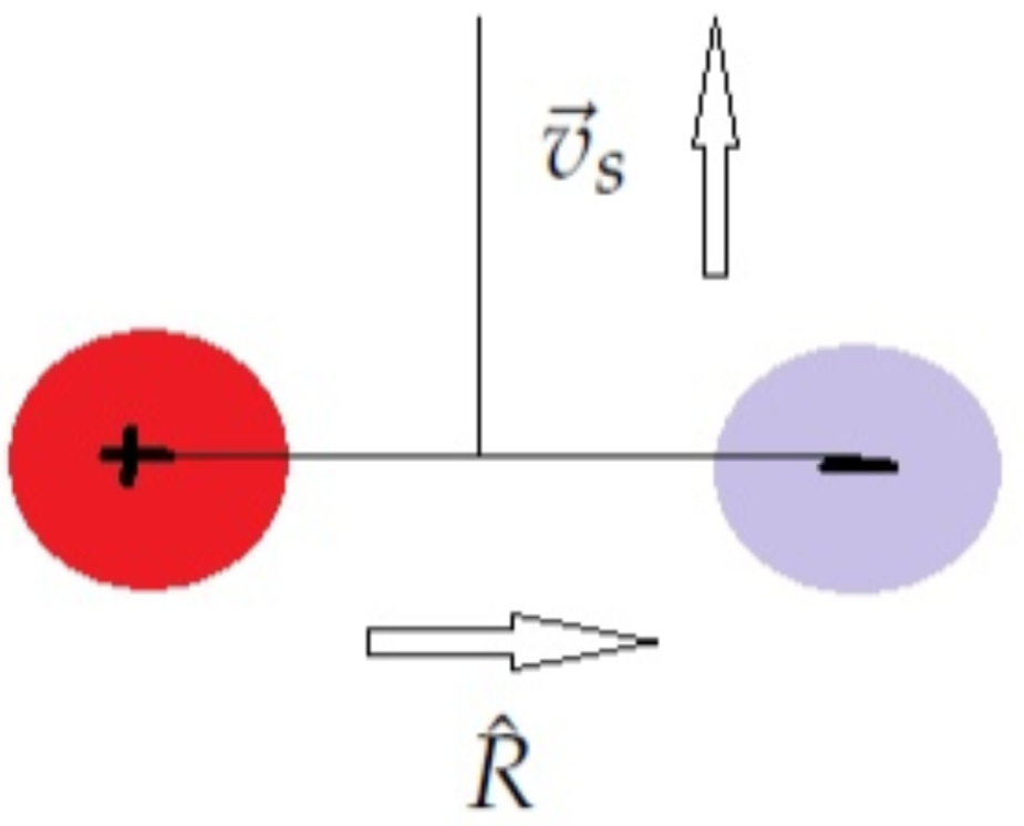
Let us assume a system consisting of two point charges such that (see Figure 3):
in which is a three dimensional Dirac delta function.
Thus Equation (76) takes the form:
Now, if the velocity is set during the system charging to be perpendicular to the vector we obtain simply:
Or according to Equation (79) we obtain, regardless of the velocity the equation:
This can only be satisfied if the displacement between the charges is fixed: , and the charges are of opposite signs, which is the case for charges in a capacitor. In this case:
If the charges are equal in magnitude by opposite in sign: we obtain the condition:
that is the rest mass energy of the device must be equal to its electrostatic energy. This is a very stringent condition and thus a more easy implementation will involve currents in the engine’s frame (and not just with respect to the laboratory), those may be either charge currents of magnetic currents. Indeed in [1] we describe a relativistic engine based on a capacitor/electret and coil carrying current. In [23] we describe a relativistic engine based on two wires carrying periodic currents, while in [24] we describe a relativistic engine composed of a permanent magnet (carrying a magnetic current) and a capacitor.
6. Conclusions
In conclusion, we investigate the legitimacy of momentum conservation concerning a charged retarded engine in this paper. We take into account the non linearity of the electromagnetic linear momentum which is proportional to the integral of the vector multiplication of the electric and magnetic fields. Although Maxwell’s electromagnetism is linear in charge and current densities the unique characteristics of linear momentum of electromagnetic fields makes this specific quantity somewhat reminiscent of the convective part of the material derivative of fluid dynamics which is quadratic in the velocity field and thus has profound nonlinear consequences, see for example [25,26].
We make use of Jefimenko’s field expression for the electric and magnetic fields in which the field sources are time dependent. This is of course a common situation in nature and it entails taking into account retardation phenomena. With these formulae, we determine the momentum acquired by the electromagnetic fields. When accounting for both the momentum of the field and the mechanical momentum of the device’s material component, conservation of momentum is upheld. Therefore, the charged retarded motor is capable of generating forward momentum independently of any external forces, solely through interaction with its own electromagnetic field. Thus, this paper has explored the principles of linear momentum conservation in charged retarded systems. This system offers a ground breaking method for space propulsion, aiming to address the major drawbacks of conventional rocket fuel. By harnessing the power of electromagnetic fields, spacecraft fitted with these engines could achieve greater speeds and distances while using significantly less fuel, thereby making interplanetary and interstellar travel more achievable.
The main scientific result of this paper is the demonstration that a relativistic engine does not violate the laws of conservation of linear momentum in fact the total linear momentum remains null. This is so because the total momentum is the sum of the linear mechanical momentum and the electromagnetic linear momentum which are always equal in size and opposite in direction to each other in a relativistic engine.
Suggestion for practical implementation as well as recommendations for designers and engineers using the principles of linear momentum conservation in charged lagging systems are given in a few published papers. In [1] we describe a relativistic engine based on a capacitor/electret and coil. In [23] we describe a relativistic engine based on two wires carrying periodic currents, while in [24] we describe a relativistic engine composed of a permanent magnet and a capacitor. Suggestions for implementations involving material design are given in [11,12].
Funding
This research received no external funding.
Data Availability Statement
No new data were created or analyzed in this study. Data sharing is not applicable to this article.
Conflicts of Interest
The authors declare no conflict of interest.
References
- Rajput, S.; Yahalom, A. Newton’s Third Law in the Framework of Special Relativity for Charged Bodies. Symmetry 2021, 13, 1250. [Google Scholar] [CrossRef]
- Yahalom, M.T. .A. Newton’s Third Law in the Framework of Special Relativity. The European Physical Journal Plus 2014, 129, 240. [Google Scholar]
- Tuval, M.; Yahalom, A. Momentum conservation in a relativistic engine. The European Physical Journal Plus 2016, 131, 1–12. [Google Scholar] [CrossRef]
- Newton, I. Philosophiae naturalis principia mathematica; Vol. 1, S. PEPYS; Reg. Soc. PRÆSES: London, England, 1687. [Google Scholar]
- Goldstein P, P.C.J.; JL, S. Classical Mechanics; Pearson; 3 edition: London, England, 2001. [Google Scholar]
- Arya, A. Introduction to Classical Mechanics; Allyn and Bacon: Boston, MA, USA, 1990. [Google Scholar]
- Jackson, J.D. Classical electrodynamics, ed., 3rd ed.; Wiley: New York, NY, 1999. [Google Scholar]
- Einstein, A. On the electrodynamics of moving bodies 1905.
- Feynman, R.P.; Leighton, R.B.; Sands, M. The Feynman lectures on physics, Vol. I: The new millennium edition: mainly mechanics, radiation, and heat; Vol. 1, Basic books: New York,New York,USA, 2011.
- D’Abramo, G. On apparent faster-than-light behavior of moving electric fields. The European Physical Journal Plus 2021, 136, 301. [Google Scholar] [CrossRef]
- Yahalom, A. Newton’s Third Law in the Framework of Special Relativity for Charged Bodies Part 2: Preliminary Analysis of a Nano Relativistic Motor. Symmetry 2022, 14, 94. [Google Scholar] [CrossRef]
- Yahalom, A. Implementing a Relativistic Motor over Atomic Scales. Symmetry 2023, 15, 1613. [Google Scholar] [CrossRef]
- Griffiths, D.J.; Heald, M.A. Time-dependent generalizations of the Biot–Savart and Coulomb laws. American Journal of Physics 1991, 59, 111–117. [Google Scholar] [CrossRef]
- Jefimenko, O. Electricity and Magnetism 2nd edn; Electret Scientific: Star City, WV:, 1989. [Google Scholar]
- Yahalom, A. Retardation in Special Relativity and the Design of a Relativistic Engine. Acta Physica Polonica A 2017, 131, 1285–1288. [Google Scholar] [CrossRef]
- Rajput, S.; Yahalom, A.; Qin, H. Lorentz symmetry group, retardation and energy transformations in a relativistic engine. Symmetry 2021, 13, 420. [Google Scholar] [CrossRef]
- Breitenberger, E. Magnetic interaction between charged particles. American Journal of Physics 1968, 36, 505–515. [Google Scholar] [CrossRef]
- Scanio, J. Conservation of momentum in electrodynamics - an example. American Journal of Physics 1975, 43, 258–260. [Google Scholar] [CrossRef]
- Portis, A. Electromagnetic Fields, Source and Media; John Wiley & Sons Inc: New-York, NY, USA, 1978. [Google Scholar]
- Jefimenko, O. A Relativistic Paradox Seemingly Violating Conservation of Momentum in Electromagnetic Systems. Eur. J. Phys. 1999, 20, 39. [Google Scholar] [CrossRef]
- Jefimenko, O. Cuasality, Electromagnetic Induction and Gravitation 2nd edn; Electret Scientific: Star City, WV:, 2000. [Google Scholar]
- Yahalom, A. Quantum Retarded Field Engine. Symmetry 2024, 16, 1109. [Google Scholar] [CrossRef]
- Yahalom, A. Time-Dependent Retarded Microwave Electromagnetic Motors. Appl. Sci. 2024, 14, 10975. [Google Scholar] [CrossRef]
- Sharma, P.; Yahalom, A. A Charged Relativistic Engine Based on a Permanent Magnet. Appl. Sci. 2024, 14, 11764. [Google Scholar] [CrossRef]
- Gao, X.Y. Auto-Bäcklund Transformation with the Solitons and Similarity Reductions for a Generalized Nonlinear Shallow Water Wave Equation. Qualitative Theory of Dynamical Systems 2024, 23, 181. [Google Scholar] [CrossRef]
- Gao, X.Y. In plasma physics and fluid dynamics: Symbolic computation on a (2+1)-dimensional variable-coefficient Sawada-Kotera system. Applied Mathematics Letters 2025, 159, 109262. [Google Scholar] [CrossRef]
Figure 1.
A change is introduced momentarily to after which it becomes static.
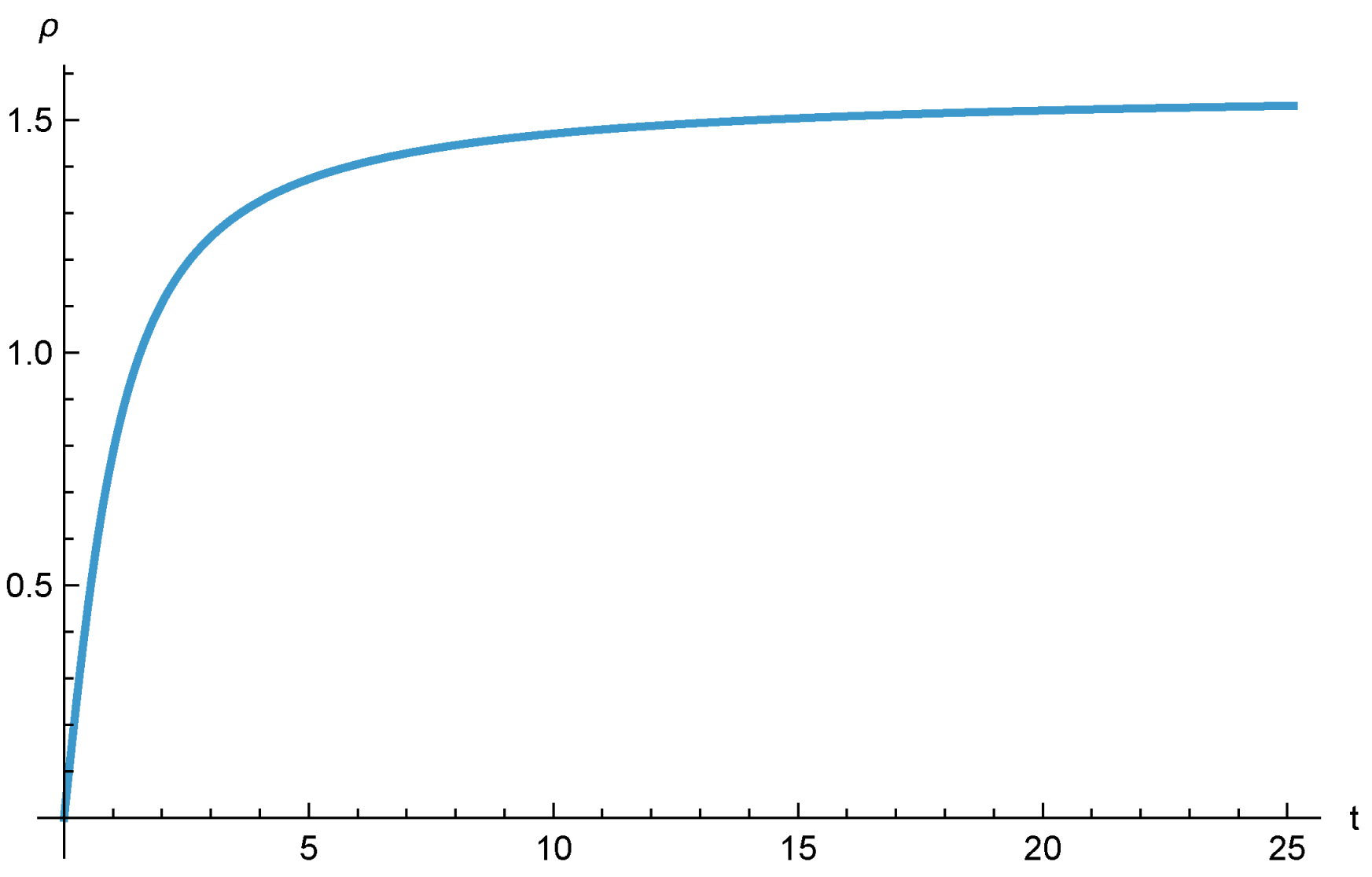
Figure 2.
The Retarded field engine comprised of charged subsystems 1 and 2, the engine is located at with respect to the inertial system.
Figure 2.
The Retarded field engine comprised of charged subsystems 1 and 2, the engine is located at with respect to the inertial system.
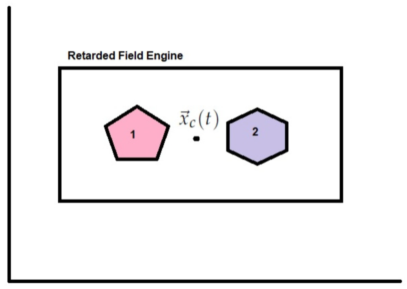
Figure 3.
Two point charges. The difference between there displacement vector is perpendicular the velocity of the system.
Figure 3.
Two point charges. The difference between there displacement vector is perpendicular the velocity of the system.
Disclaimer/Publisher’s Note: The statements, opinions and data contained in all publications are solely those of the individual author(s) and contributor(s) and not of MDPI and/or the editor(s). MDPI and/or the editor(s) disclaim responsibility for any injury to people or property resulting from any ideas, methods, instructions or products referred to in the content. |
© 2025 by the authors. Licensee MDPI, Basel, Switzerland. This article is an open access article distributed under the terms and conditions of the Creative Commons Attribution (CC BY) license (http://creativecommons.org/licenses/by/4.0/).
Copyright: This open access article is published under a Creative Commons CC BY 4.0 license, which permit the free download, distribution, and reuse, provided that the author and preprint are cited in any reuse.


