
Submitted:
08 July 2025
Posted:
09 July 2025
You are already at the latest version
Abstract
In multibody systems (MBS), such as robot structures, classical modeling is often based on simplified assumptions concerning mass geometry.
This paper introduces a formal theoretical model to overcome these limitations by in-troducing the concept of mass distribution, which describes the continuous nature of mass properties within kinetic assemblies. Furthermore, the research integrates high-er-order acceleration energies into the dynamic formulation – a topic less explored in conventional approaches. By applying the principles of analytical dynamics, particularly a generalized form of D'Alembert-Lagrange principle, a comprehensive model based on higher-order acceleration energies is developed. Matrix exponentials and higher-order differential operators are applied to determine the dynamic equations. Generalized forces are also analyzed as essential dynamical parameters, directly related to general-ized variables and characterized by mass properties, including mass centers, inertial tensors, and pseudo-inertial tensors. The dynamic behavior of the system is described by using matrix-based expressions for defining kinetic and acceleration energies, and their time derivatives.
The paper proposes a unified, matrix-based theoretical framework for modeling ad-vanced dynamics in MBS, emphasizing the role of mass distribution and higher-order acceleration energies. This formulation facilitates a deeper understanding of inertial properties and dynamic interactions in complex mechanical systems such as robots.
Keywords:
acceleration energies
; mass distribution
; dynamics
; generalized forces
1. Introduction
In recent years, the development of dynamic models for mechanical systems has evolved toward more accurate and universally adaptable formulations. This shift reflects the increasing complexity of engineering applications, particularly in fields like robotics, aerospace, and flexible multibody systems. In such systems, traditional simplifications – such as modeling discrete masses and neglecting higher – order acceleration – fail to capture critical effects inherent to complex behaviors. Within this context, three central aspects have emerged as essential for accurate modeling: mass distribution, higher-order acceleration energies, and generalized forces.
Mass distribution significantly affects system dynamics, especially flexible structures or spatial linkages. Unlike models based solely on discrete parameters, mass distribution models allow for spatial variation of inertia and stiffness. This capability leads to improved accuracy in analyzing the local dynamics, internal wave propagation, and modal coupling effects.
Mizhidon [1] introduced a unified mathematical framework that incorporates both discrete and distributed parameters yielding a more realistic representation of mechanical systems. His model enhances predictions of deformation and energy transfer across structural elements with variable density and elasticity.
Similarly, Yang et al. [2] proposed a multiscale approach for flexible multibody systems, integrating spatially distributed mass and stiffness parameters. Their findings demonstrate that neglecting distributed effects introduces systematic errors in dynamic simulations, particularly in high-frequency or transient regimes.
In classical dynamics, kinetic energy is typically defined based on velocities, i.e., first-order derivatives. However, in systems subjected to sudden accelerations, shocks, or control input variations, higher-order derivatives such as jerk or snap become relevant. Negrean, Crișan, and Vlase [3,4] have introduced theoretical formulations that incorporate these acceleration energies within the analytical mechanics framework. Specifically, they extended the classical Lagrangian and Gibbs-Appell equations to include second- and third-order time derivatives of the acceleration energies.
In a subsequent study [5], the same authors extend the formulation on kinetic and acceleration energy expressions and propose new formulations for generalized variables based on higher-order derivatives. The concept of generalized forces is proposed as an extension of d’Alembert Principle, adapted for systems characterized by higher order accelerations. Similarly, de Jong et al. [6] derived dynamic equations for rigid body spatial mechanisms incorporating higher-order derivatives, demonstrating that dynamic balancing – often addressed heuristically – can be treated rigorously handled using analytical models based on jerk and snap. Generalized forces thus became central in advanced dynamic. These are not limited to some functions of displacement and velocity but can involve accelerations and their derivatives. Jafari et al. [7] presented a flexible-link robot model that integrates generalized forces derived from both structural compliance and control feedback mechanisms. Their model improves stability and accuracy, particularly under high-speed motion or external influences.
Complementarily, Condurache [8] conducted a theoretical study on the effects of higher-order accelerations in the dynamic behavior of mechanical linkages. He demonstrated that forces transmitted through joints and links must be defined with respect to time derivatives of acceleration, especially in high-speed motion regimes.
This perspective creates opportunities for developing different control strategies and optimization algorithms based on higher-order acceleration energies.
In the present paper, the simultaneous evaluation of mass distribution, higher-order acceleration energies, and generalized forces lead to a more comprehensive and reliable modeling approach. The work aims to synthesize recent theoretical advancements and develop a unified dynamic model applicable to mechanical systems with distributed mass and inertia, while preserving rigid body assumptions.
2. Mass Distribution in the Dynamics of Mechanical Systems
In multibody systems (MBS), such as robotic mechanical structures, it is common to adopt simplifying assumptions concerning mass properties. A frequently applied hypothesis is that the mass is continuously distributed throughout the entire mechanical structure—from the fixed base to the final kinetic assembly. Based on this assumption, the present study adopts the term “mass distribution” as a more accurate descriptor than the traditional expression “mass geometry,” which typically refers to ideal rigid bodies.
According to classical Newtonian dynamics, inertia in the translational motion is iis characterized by the system’s mass and the position of its center of mass while rotational inertia is defined by the mechanical moments of inertia—originally formalized by Leonhard Euler in 1758 — and further extended through the inertia tensor and the pseudo-inertia tensor [9]-[14].
These matrix representations are fundamental in defining dynamic quantities such as angular momentum, kinetic energy, higher-order acceleration energies, and their respective time derivatives, as required by the formulation of higher-order differential equations characteristic of analytical dynamics [15,16,17,18,19].
In this study, the authors further develop the concept of mass distribution (MD – type) based on prior work presented in [4,5]. To facilitate the analysis, several simplifying assumptions are introduced. Each kinetic subassembly, within the multibody system (MBS), is modeled as a rigid body, (see Figure 1).
At the same time, MD-type properties are using the mass and geometric integrals which are applicable exclusively to homogeneous bodies with simple or regular geometric shapes. A homogeneous body is, by definition, characterized by a constant density over an infinite number of infinitesimal mass elements, continuously spread throughout its geometry. In most cases, each kinetic subassembly is a compound body with an irregular geometric shape, which makes the direct application of mass integrals impossible.
As an illustrative example, the kinetic ensemble , presented in Figure 1 as part of the multibody system (MBS) is considered.
Its geometrical decomposition is detailed in Figure 2.
Based on the considerations above, each kinetic ensemble is decomposed into a finite number of homogeneous bodies with simple or regular geometrical shapes, denoted as , with , where .
The kinetic subassembly presented in Figure 2 is decomposed into simpler components , each assumed to have regular geometry and uniform density. This decomposition facilitates the computation of mass distribution properties such as center of mass, inertia tensor, and pseudo-inertial tensor for the full subassembly. To each component body a local reference frame centered at its geometric centroid is attached. Additionally, for each kinetic ensemble, a dedicated coordinate frameis defined at the geometric center of its corresponding joint, enabling consistent formulation of dynamic equations within the multibody system.
Based on these assumptions and the authors’ previous formulations, this section develops the mass distribution properties associated with such systems. These properties include: the total mass and the position of the center of masses, mechanical moments of inertia (axial, planar, polar, and products of inertia); the inertia tensor together with its generalized variation law; and the pseudo-inertia tensor, as detailed in [3,4,5].
The total mass and the position of the center of mass are first calculated for each component bodyas illustrated by the example in Figure 3:
A consistent formulation of mass distribution properties requires a clear definition of the differential mass element which integrate density and geometry into a unified framework applicable to different body types, including linear, surface, and volumetric structures.
To this end, the concept of is generalized as follows:
where is the linear density characteristic to one – dimensional (1D) components such as rods or beams; denotes the surface density applicable to two – dimensional (2D) elements such as plates or shells and represents the volumetric density, and is used for three – dimensional (3D) bodies.
This unified definition allows the computation of mass – related properties to be expressed in an integral form applicable to a wide variety of bodies with varying geometry and dimensions (1D, 2D or 3D).
According to [3,4,5], the position vector of the center of masses is defined by:
where is the system attached to the mass center of the simple homogenous body part of kinetic element and is the mass of the body , given by:
and is substituted by (1) as a function of body’s geometry.
The position of the center of mass must be expressed relative to the frames or which are associated with the kinematic structure of the multibody system (MBS). Consequently, the expressions are rewritten as follows:
The global center of masses for the kinetic ensemble , denoted , is computed as a mass weighted average of its component bodies’ centers of mass.
The defining expression considers the additive and subtractive contributions of each component through the sign of operator :
if the component belongs to subassembly and
when the component is subtracted from subassembly (e.g., a cavity or excluded region). The position vector defines the positioning of subassembly relative to fixed frame or , as presented below:
where sometimes is recommended.
The symbol expresses the rotation and respectively locating matrix between frames and or (see also Figure 4).
Considering that the subassembly has been decomposed into simple bodies , the application of expressions (2)-(4) to each component allows the computation of the total mass and position of the mass center of the kinetic ensemble .
The parameter represents the number of simple bodies resulting from the decomposition of subassembly and the final expressions are given as follows:
Equation (6) defines the total mass of the kinetic ensemble, while Equation (5) provides the position vector of mass center.
2.1. The Inertial Tensor in Case of a Rigid Body
When a kinetic ensemble, from a multibody system is characterized by resultant rotational motion, its inertia properties are primarily expressed through mechanical moments of inertia and their extended representations, namely the inertial tensor and pseudo-inertia tensor [3,4]. Following the same approach used in the previous section, these inertia – related properties will first be determined for each homogeneous component body. An illustrative example is shown in Figure 3.
Each homogeneous body has already been analyzed in terms of its mass (see Equation (2)) and position of the mass center (Equations (3)–(5)). According to Figure 3, the mass center of the body (denoted ) serves as the origin of three concurrent frames, which are described below:
Considering the formulations of the authors, a few symbols and notations are used:
where in Equation(9), the symbols refer to the Cartesian coordinates or axes of the local reference frames. Expressions (10)-(12) define the unit vectors that describe the orientation between the frames , and or between,, andrespectively.
Based on these definitions, the rotation matrix can be expressed as follows:
To express the inertia properties for each homogenous body relative to its own mass center, the local coordinate system is positioned such that its origin coincides with the center of masses, thus leading to the following condition:
where represents the position vector of a mass element relative to the mass center of body , relative to a local frame.
Additionally, the coordinate transformation between the frame attached to body and the reference frame corresponding to of ensemble or the frame attached to the fixed basis of the robot, is defined by the following relations:
where Equation (15) defines the position of bodyrelative to frames: .
Equation (15) is rewritten below as follows:
Another notation, essential in the present formulation, is the skew symmetric matrix associated with the position vector defined in Equation (14), as well as its transpose:
To determine the inertia properties in either frameor, the position of a mass element is given by the following expressions:
where Equation(19) shows the position of elementary mass in homogeneous coordinates.
Since each homogeneous body is assumed to have simple geometrical shape, its moment of inertia can be expressed as a mass integral, as established in references [3,4,5,6,7,8,9]. This integral involves the product of the differential mass element and the square of its distance from a given axis or plane, and is defined as follows:
,
Accordingly, the axial, centrifugal and planar mechanical moments of inertia relative to frame are known, and are included in the following set:
In the next step, the axial, centrifugal and planar mechanical moments of inertia with respect to , must be computed by considering the following:
The squared distance from a mass element to an axis defined by the unit vector (see Figure 3) is determined according to the following expression:
As a result, based on Equations (21)-(24), the axial mechanical moment of inertia is given by:
However, the mechanical moments of inertia, defined in Equation (21) can also be computed using the coordinates included in the transfer matrix formulation (16), as follows:
The squared distance between a differential mass element and the mass center is mathematically defined as:
In Equation (26) the sum of the squared components of the position vector is reformulated as a scalar product allowing compact matrix representation:
Substituting Equation(28) in Equation(26), expressions become:
Consequently, the mechanical moment of inertia in Equation (25) can be reformulated using the relations provided in Equation (24) or (32), as follows:
The corresponding mass integral from (25) or (33) is expressed symbolically as follows:
In the matrix (34), the main diagonal contains the axial moments of inertia, while off – diagonal terms – symmetric and with negative sign – correspond to centrifugal moments of inertia (products of inertia). According to [2,3,4], the matrix in Equation (34) is known as the inertia tensor (axial and centrifugal) of body with respect to frame evaluated at its center of masses . Based on this inertia tensor, symbolized by (34), the axial mechanical moment of inertia relative to frames is determined as:
Based on the definitions provided in Equations (23) and (21),the centrifugal moment of inertia is computed as follows:
The matrix, defined by Equation (28) is rewritten as presented below:
When substituted in Equation (37), this expression leads to the following transformation:
where (34) has been substituted.
Using Equation (13) and its transpose, the centrifugal moments of inertia become:
Equation (36) and (41) are included in the matrix of axial and centrifugal moments of inertia:
The matrices defined in Equations (42) and (43), presented in their expanded form, constitute the inertia tensor axial and centrifugal of the body relative to frame and evaluated at the mass center. Simultaneously, these expressions represent the variation law of the inertia tensor with respect to concurrent reference frames located at the mass center . Based on Equation (22) and (23), the following section addresses the computation of the planar moment of inertia, as defined by:
By substituting Equation (38) into Equation (44) and evaluating the mass integrals, the following result is obtained:
The matrix of inertia moments defined in Equation (45) is referred to as the planar and centrifugal inertia tensor of body relative to reference frame and applied at the mass center. Based on this tensor representation, the planar mechanical moments of inertia of body relative to frame are determined as:
Based on Equation (41), in which the inertia tensor from Equation (45) is substituted, the centrifugal moments of inertia are determined using the following expressions:
Therefore, Equations (47) and (48) are included into a matrix that represents the planar and centrifugal moments of inertia:
The matrices defined in Equations (49) and (50), in their expanded form, represent the planar – centrifugal inertia tensor of body relative to reference frame applied at its center of masses . At the same time, Equations (42) and (43) describe the variation law of the inertia tensor with respect to concurrent reference frames located at the mass center .
In many cases, the fundamental concepts and theorems of analytical dynamics are expressed in a matrix form. Therefore, the position vectors from Equation (19) are rewritten using homogeneous coordinates, which leads to the following matrix representation:
In this formulation, Equation (14) is substituted, incorporating the planar – centrifugal inertia tensor (from Equation (45)), the static moments and the mass of the body. The resulting matrix defines the pseudo-inertia tensor of the body relative to reference frame , applied at the mass center. Accordingly, the expression of the pseudo-inertia tensor relative to frame is given by:
where the conditions (14) are substituted again. But, (52) can be written in another form:
The square matrix defined in Equation (53), symmetric and positive defined, represents the variation law of the pseudo-inertial tensor with respect to concurrent reference frames located at the mass center . The matrix defined with (54) is the homogenous transformation matrix which is used to determine a pure rotation from frame to frame . The components of this matrix are represented by which is the rotation matrix that characterizes the rotation of frame relative to frames or . The rightmost column of the homogenous transformation and the bottom row contain zeros and a scalar 1. The matrix does not include translation, making it a pure rotational transformation into homogenous space.
2.2. The Generalized Variation of the Inertial Tensor
The mass properties for any homogeneous body assumed to have a simple geometric configuration [2], can be determined from the following predefined parameters:
Based on the expressions provided in Section 2 of this paper, the mass properties are computed relative to reference frame, as follows:
.
In the following steps, the axial, centrifugal and planar mechanical moments of inertia for each homogeneous body are to be computed with respect to frames and , in accordance with the kinematic structure of MBS (as presented in Figure 1):
These quantities are included in the generalized variation law of the inertial and pseudo-inertial tensors, as presented below:
To begin with, the generalized variation law of the axial and centrifugal inertia tensor for body relative to reference frameis determined as follows:
The expression given in Equation (59) is referred to as the axial and centrifugal inertia matrix of the mass center relative to reference frames.
Based on Equation (57), the generalized variation law for the planar and centrifugal inertia tensor of the body relative to frame is formulated as follows:
The expression (84) defines the planar and centrifugal inertia matrix evaluated at the mass center , with respect to the frames.
The pseudo – inertia tensor variation law of the body with respect to frames , obtained from Equations (51)-(53), is given below:
is the locating matrix between frames versus .
2.3. The Inertial Tensor for Multibody Systems (MBS)
The generalized variation laws of the inertial and pseudo-inertial tensors, as defined in Equation (57), have been defined for every homogeneous body relative to frames. In this section, based on the previously established expressions, the inertia properties for each kinetic ensemblewill be determined. These include the axial, centrifugal and planar mechanical moments of inertia, in accordance with the models presented in references [4] and [5]:
These values, already defined, are now included in the expressions for the inertial and pseudo-inertial tensors:
Therefore, the generalized variation law for the axial and centrifugal inertia tensor of the kinetic ensemble relative to frameis determined below:
The generalized variation law of the planar and centrifugal inertia tensor of the kinetic ensemble, relative to reference frame, is established with expressions:
Following the formulation presented in Equation (65), the pseudo-inertial tensor corresponding to the kinetic ensemble relative to framesis determined as:
The expression defined above contains the planar and centrifugal inertia tensor (as presented in Equation (69)), along with the static moments (Equation (5)) and the total mass (from Equation (6)) of the kinetic ensemble.
3. The Acceleration Energies of Higher Order
Unlike other research papers addressing these advanced concepts, the main objective of this section is to present, in a matrix form, the fundamental expressions defining the higher – order acceleration energies. By applying the differential principle in generalized form (a generalization of the Lagrange–D’Alembert principle), the dynamic equations of fast-moving mechanical systems naturally incorporate these higher-order acceleration energies. As documented in the scientific literature [20,21,22], the foundations of these equations were laid in 1879 by J. W. Gibbs who formulated the differential equations of motion. Subsequently, in 1899, Paul Appell extended this work through a more elaborate analysis [23,24]. The outcome of this development is a set of equations now known as Gibbs–Appell equations. These equations are applied to holonomic and non-holonomic systems.
The study presented in this section was carried out by considering the holonomic mechanical systems, for which, the Gibbs–Appell equations along with their higher-order derivatives, are refined to suit this type of systems. Furthermore, this section emphasizes the importance of higher acceleration energies as central functions, in the analysis of the dynamics of high – speed mechanical systems.
In this framework, the kinetic energy is substituted by the acceleration energy, also referred to as Appell’s function or “kinetic energy of acceleration” [3,5].
Unlike the studies mentioned above, the authors have developed explicit expressions for the first, second, and third – order acceleration energy, specific to mechanical systems characterized by high – speed motions [18].
To determine the general expressions for the acceleration energies of pth order, the corresponding differential matrices are introduced in the following subsection.
3.1. The Differential Matrices in the Advanced Kinematics
Based on the formulations of homogenous transformations and matrix exponentials, the differential matrices of these homogeneous transformations are developed. These matrices – also known as dynamics matrices – are essential components in the matrix representation of the acceleration energies, particularly for mechanical systems characterized by fast motions. As stated in [18], the dynamics matrices comprise first-, second- and higher – order differential matrices, which can be determined either by directly applying the partial derivatives to the homogenous transformations or by using the properties of matrix exponential functions.
The components of the differential matrices are represented by the submatrices corresponding to the rotation and position , respectively. The first-order differential matrices, representing the time derivatives of the homogenous transformations are obtained as follows:
By employing the matrix exponentials formalism, the two components represented by the rotation transformation , and position , from Equation (71), are further defined:
The differential matrix of second order is defined with matrix exponential functions:
The sub-matrices included in Equation (72) and (79) are determined according to [3,4,5], by using matrix exponential functions. The following symbols are explained:
represents the derivative matrix operator (Uicker operator).
- it represents the unit vector of the driving axis in the initial configuration (zero)
- it represents the generalized variable of the driving axis.
and defines the position vector in the initial configuration and the orientation matrix of the system relative to , respectively;
- it represents the 4th column of the exponential of a homogeneous transformation and is defined according to [25], as follows:
- is a screw parameter or one of the homogeneous coordinates of the driving axis.
The first- and second- order differential matrices, previously introduced as reference expressions, play an essential in establishing dynamics matrices.
These dynamics matrices are key components in the matrix formulations that define higher – order acceleration energies.
3.2. The Matrix Expressions for the Acceleration Energies
The following relations are the starting point for the formulation of acceleration energy:
Equation (82) defines the acceleration energy of order for the entire mechanical system. The notations used in this equation have the following meaning:
and represent the order of the absolute time derivatives,is the position vector of the elementary mass , relative to a reference frame located at the mass center; is the position vector of the mass center, projected onto the fixed or moving frame; is the orientation matrix between the two reference systems.
The mechanical system is characterized bydegrees of freedom (d.o.f.) or generalized coordinates, which are included in the column matrix .
It should be noted that the explicit expressions for the higher – order acceleration energies were previously determined in [4], using mass integrals.
In this section, only the matrix form of the higher orders acceleration energies is presented.
3.3. TheAcceleration Energies of the First Order
Starting from Equation (82) and applying a series of successive matrix transformations, the defining expression for the first – order acceleration energy of is obtained. This expression can be represented in the following matrix form:
Equation (83) includes the column vector of the generalized velocities and accelerations, whose components correspond to the first- and second – order time derivatives of the column matrix of generalized variables .
Additionally, within Equation (83) a set of dynamics matrices can be identified.
These matrices are defined as follows:
Equation (84) defines a matrix, commonly referred to as the mass matrix or the inertia matrix associated with the first – order acceleration energy. Its components denoted by are explicitly defined in the same context. The column matrix of centrifugal and Coriolis terms of the first-order is defined by Equation(86), and is represented as an matrix, with the following components:
The pseudo inertial matrix corresponding to the acceleration energies of first order is defined as follows:
The formulations in Equations (83) and (87) include the differential matrices of first and second-order denoted with and, respectively. These are computed via the Equations (71)–(74) in the case of the differential matrices of first-order (), while for the differential matrices of second order, the Equations (76)–(79) are applied.
3.3. The Acceleration Energy of Second-Order
As demonstrated in the authors’ previous research [3,4,5], sudden motions, transient motion phases, and the mechanical systems subjected to the action of a system of external forces, with a time variation law, are characterized by higher order linear and angular accelerations.
More specifically, fast – moving mechanical systems, which are subjected to the action of external forces with time variation law, are characterized by higher order linear and angular accelerations.
Unlike the formulations presented in [4], where the second – order acceleration energy of the was established using mass integrals, the following expression introduces a matrix – based formulation of the second – order acceleration energy, as:
The components and are not developed in this paper. Their components in explicit form can be found in the research presented in [4]. Equation (88) includes the dynamics matrices of the second order. These are defined as:
Therefore, both the inertia matrix and the matrix of Coriolis and centrifugal terms, are components in the expression of the second – order acceleration energy.
3.4. The Acceleration Energy of Third-Order
The dynamic analysis is further extended to include the third – order acceleration energy. As previously stated, the explicit integral formulation of the third – order acceleration energy was presented in [4]. According to the approach introduced in [3], the matrix form of the third – order, defined as a function which depends exclusively on , is given as follows:
The dynamics matrices of the third order, included in the acceleration energy of third order, are defined by the following expressions:
It is important to note that, in case of third – order acceleration energy, the mass properties are characterized by the pseudo – inertial tensor and higher-order differential matrices.
3.5. The Acceleration Energy of p-th-Order
For multibody mechanical systems, the fourth-order acceleration energy becomes a central function , in the dynamic formulation. The corresponding expression is given as follows:
The acceleration energy of pth order can be established According to the models outlined in [5,18], its corresponding expression is given below:
In the expression of higher-order acceleration energy, the contribution of mass properties is reflected through the presence pseudo – inertial tensor. The tensor is a key component of the dynamics matrices, which were previously introduced and defined in Equations (84), (87) and (89).
4. The Generalized Forces in the Dynamics of Systems
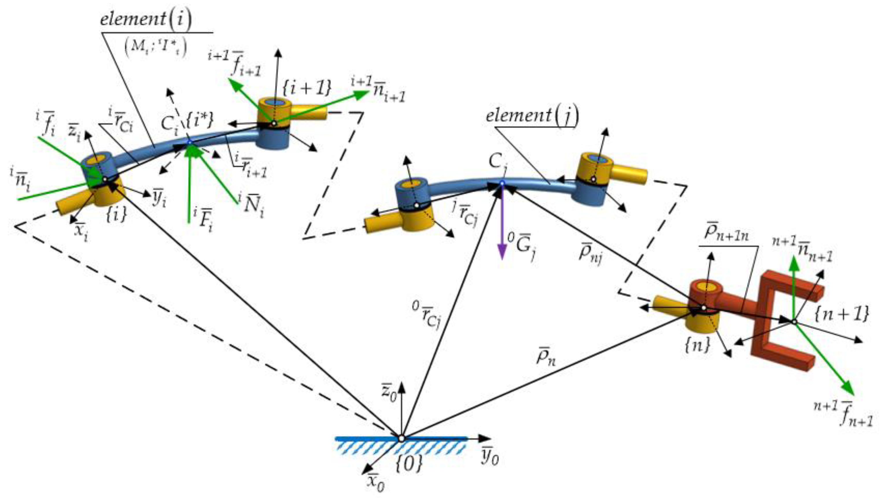
In accordance with differential principles typical to analytical dynamics of systems, the study of a system’s dynamical behavior fundamentally relies on the concept of generalized forces. These forces are mechanically developed in direct relation to the generalized variables, also referred to as independent parameters or degrees of freedom (d.o.f.) which uniquely describe the absolute motion of holonomic mechanical systems. From a mechanical perspective, the generalized forces are due to various sources including actuation mechanisms, gravitational fields, manipulating loads, as well as complex frictional effects associated with physical connections between kinetic subassemblies in a MBS – as illustrated in Figure 4 and Figure 5.
According to [3,4,18], each kinetic ensemble , that is a part of the mechanical structure of a robot, and implicitly integrated within the multibody system (MBS), is subject to a system of external and active forces, manipulating loads, and complex frictional effects, as seen in Figure 4.
Depending on the behavior (whether static or dynamic) of each physical link – particularly within driving joints of fifth order – a corresponding generalized force is generated. This may take the form of a generalized static force or a generalized actuation force, depending on the context of motion and interaction.
4.1. The Generalized Static Forces
To begin with and by following the classical algorithm described in [4,5], the generalized forces corresponding to static equilibrium are determined. Based on the fundamental theorems of statics applied to mechanical systems, and after performing a few transformations, the following expressions are obtained for the constraint force and for the corresponding moment of the constraint forces :
where is the unit vector of (the gravity acceleration vector).
The operator defined in Equation (96) serves to highlight two types of external loads: gravitational loads denoted by and manipulating loads represented by symbol. The equations (94) and (95) are established through outward iterations , following the model described in [4,5]. These expressions are then substituted in the formulation of the generalized static force, yielding to the following result:
where the quantities and represent the generalized gravitational and manipulating forces, respectively, as defined in [25]. They are commonly referred to as generalized active forces. Unlike the classical formulation based on the principle of virtual work, the approach adopted here – as detailed in [5,18,25] – determines these forces using transfer matrices for linear and angular velocities. Based on Equations (94), (95) and (99), the starting equation for the generalized gravitational force is given by:
Considering the transfer matrices for linear and angular velocities, as detailed in [25], a set of transformations is carried out to determine the generalized gravitational force. These transformations are presented as follows:
The column vectors (101) – (103) are components of the Jacobian matrix, according with:
where
The same components of the Jacobian matrix can alternatively be determined using matrix exponentials, as detailed in [25,26]. The corresponding expressions are provided below:
Parameters from Equations (107) and (108) maintain the same definitions provided in § 3.1.
Based on these, the defining formulation for the generalized gravitational force results:
The column vector defined in Equation (110), expressed in Cartesian space, is mechanically equivalent to the wrench (i.e., the combined resultant force and moment) generated by the gravitational forces acting on the interval relative to the moving reference frame, attached to the geometric center of the final driving joint from MBS, as illustrated in Figure 4. Following the expressions (94), (95) and (99), the starting equation for the generalized manipulating force is given as:
4.2. The Generalized Dynamics Forces
Considering the aspects presented in [25], in the context of the dynamical behavior of multibody systems (MBS), each driving joint is subjected not only to the active forces, discussed in the previous subsection, but also to the effects of generalized inertia and driving forces. The determination of these forces constitutes the main objective of the current subsection. As a starting point, the iterative algorithm associated to the classical formulation of the dynamic equations, is applied. The traditional approach is based on the D’Alembert principle of analytical dynamics which accounts for inertia by transforming a dynamic system into a quasi-static one through the inclusion of inertial forces.
In Equations (117) and (118) one can observe the application of two fundamental theorems in dynamics of mechanical systems: the theorem of the motion of the mass center, expressed in Equation (119) and theorem of the angular momentum formulated in Equation (120):
The above expressions apply to each kinetic ensemble in the multibody system.
The involved symbols have the following physical interpretations: denotes the acceleration of mass center; and represent the resultant force and resultant moment, respectively, and is the axial and centrifugal inertia tensor defined relative to the frame which is applied at the mass center of the kinetic ensemble.
Starting from Equations (117) and (118), the following expression for the generalized driving force is obtained:
where and denote the generalized active forces, represents the generalized inertia force, and is a scalar operator used to distinguish between static and dynamic operating conditions of the system, with corresponding to static conditions and corresponding to dynamic behavior.
The starting equation for determining the generalized inertia force is:
Following the same approach as in Equation (113), the final expression of the generalized inertia force is written as follows:
The column vector defined in Equation (110), expressed in Cartesian space, is mechanically equivalent to the wrench of the inertia forces acting on the interval , with respect to the moving frame attached to the geometric center of the last driving joint in the MBS structure (see Figure 4 and Figure 5).
Consequently, the generalized driving force corresponding to each driving axis in the multibody system (MBS) is finally expressed as follows:
The generalized active and inertia forces share the same mathematical structure, which represents a significant advantage in formulating the dynamic’s equations (128) corresponding to each kinetic ensemble in the multibody system (MBS) (see Figure 5).
Considering the presence of complex friction forces acting within each driving joint of the robotic system, the corresponding generalized friction force, is defined as follows:
where the symbols: and represents the viscous friction coefficient and the dry friction coefficient, respectively both defined as a function of the joint type. Within Equation (129) the following operator is defined:
where highlights the contribution of the external loads by as well as the influence of the complex frictions.
In accordance with the mathematical aspects, previously discussed, the resultant force vector included in the generalized friction force (129) is determined as follows:
Consequently, Equation (122) is reformulated as follows:
As a result, Equation (132) for defines the system of generalized driving forces which are identical to the dynamic equations of the multibody system (MBS). These equations include the generalized active and inertia forces, as well as the complex friction effects acting within each joint. It can also evident that, in both cases – generalized gravitational forces , and generalized inertial forces – the influence of mass properties play an important role in shaping the dynamic behavior of the robot’s mechanical structure.
Furthermore, Equations (109), (114) and (128) emphasize one of the fundamental properties in analytical dynamics, namely the one related to the Jacobian matrix.
This matrix ensures, from both a mathematical and physical perspectives, the transfer of the gravitational loads, manipulation forces, and inertial wrenches – originally applied at the end-effector — to each driving axis of the robot.
5. The Higher Order Dynamic’s Equations
When mechanical systems (MBS) are subject to sudden or transitory motions, both theoretical and experimental research [25] confirms the existence and relevance of higher – order accelerations energy. These energies are incorporated into the higher – order dynamic equations, where the time variation of generalized forces becomes explicit. In the specific case of the robotic mechanical structure (see Figure 5 ) which is characterized by the sudden motions, both higher – order generalized accelerations, and the corresponding generalized forces are developed. Based on the studies in references [25,26,27,28,29,30], the following categories of higher – order derivatives are identified:
The meaning of the terms used in Equations (133) – (135) has been clearly defined in the previous sections, where is the order of time derivation. However, in the context of dynamic equations, the notation is used instead of .
When, the equations (133) – (135) reduce to the classical forms: Equation (125), Equation (109), and finally Equation (114), respectively. By applying Lagrange, Gibbs-Appell and author’s own formulations [18,25], the generalized differential equations of higher order are obtained for mechanical systems that are dynamically characterized by sudden and transient motions
The acceleration energies of first, second and third order have been defined both in the present study and in previous works [4,5,18,25].
Authors have proposed in [18], a formulation for the generalized higher – order differential equations, applicable to the mechanical systems (MBS), dynamically characterized by sudden and transient motions.
In these equations, the central function becomes the pth order acceleration energy, to which successive time derivatives of higher – order is applied, as follows:
The necessary conditions in (139) and (140) are the following:
The expression (139) which is identical in form to Equation (133), represents the order time derivative of the generalized inertia force. In the case of rapid motions, the Equation (122) is modified as follows:
Thus, a system of n higher – order differential equations is obtained, describing the dynamic behavior of robotic mechanical structures subjected to rapid and transient motions.
The research presented in this paper introduces a novel and unified formulation of the higher – order dynamic equations modeling the dynamic behavior of multibody mechanical systems, particularly of those subjected to sudden accelerations and transient motions. Unlike classical approaches limited to first – order formulations, this study systematically integrates the acceleration energies of higher – order into a matrix – based model, enabling a more accurate and physically consistent modeling of robotic structures under dynamic stress. The introduction of generalized equations of p – order, together with the use of pseudo inertial tensors and advanced dynamic matrices, represents a significant original contribution to analytical dynamics and robotic modeling.
These formulations allow the direct connection between mass properties, higher – order kinematics and generalized forces, offering a clear perspective on the dynamic performance of robotic structures.
6. Conclusions
The paper is structured into four main sections, each addressing a fundamental aspect of advanced dynamics of mechanical systems: the distribution of mass properties, the formulation of higher-order acceleration energies, the generalized forces in multibody system dynamics, and the development of higher-order dynamic equations.
The first section introduces a novel and consistent framework for analytical modeling of multibody systems (MBS), particularly applicable to robotic structures subject to rapid dynamic transitions (transient and fast motions).
A key contribution is the formulation of the mass distribution (MD) concept, which generalizes the classical notion of mass geometry and emphasizes the dual role of mass and energy in defining matter and expressing its gravitational and inertial behavior.
This leads to a rigorous definition of the essential mass properties—total mass, center of masses, inertia tensor, its generalized variation law, and the pseudo-inertial tensor—initially for homogeneous bodies with simple geometry and later extended to complex subassemblies. These properties are essential in defining key dynamic quantities such as angular momentum, kinetic energy, and higher-order acceleration energies, which play a central role in the proposed higher-order differential equations.
In the second section, higher-order acceleration energies are introduced as a main component of the proposed dynamic model. The novelty lies in the formulation of these energies in matrix form, using homogeneous transformation matrices and matrix exponentials—an approach that is distinct from classical methods. Unlike traditional approaches, this study addresses holonomic systems undergoing general motion and integrates higher-order accelerations to improve the accuracy of dynamic models.
The third section focuses on the generalized forces such as gravitational, manipulation, inertial and friction forces, formulated based on d’Alembert’s principle and Jacobian based on transfer matrices of linear and angular velocities. These forces are explicitly expressed in a generalized form, for each driving joint and adapted to include friction effects at joint level. The final section extends the authors’ previous research by introducing generalized higher – order forces and dynamic equations obtained applying the analytical dynamics principles. These results are intended to model the behavior of complex mechanical structures subject to nonstationary regimes and transient inputs.
In conclusion, the mass distribution concept, the matrix – based formulation of higher – order acceleration energies, and the extension of Gibbs – Appell equations together define a unified and original theoretical framework for advanced dynamic modeling of multibody systems (MBS).
Compared to classical Newton – Euler or Lagrangian formulations, this model offers improved capability for capturing the influence of higher – order dynamics in fast and complex motion scenarios. Moreover, the higher – order differential equations developed here are capable of time – dependent behavior, showing strong potential for future applications in real – time control and high – speed robotics.
It is important to emphasize that this is a theoretical investigation focused exclusively on mathematical formulations and symbolic generalizations without experimental validation or numerical simulations. However, the presented formulations provide a solid foundation for future validation through computational simulations and experimental testing in robotic systems.
Author Contributions
Conceptualization, I.N. and A.V.C.; methodology, I.N.; software, A.V.C.; validation, I.N., A.V.C. and R.M.G; formal analysis, I.N.; investigation, I.N., A.V.C., R.M.G; writing—original draft preparation, A.V.C.; writing—review and editing, A.V.C., I.N.; R.M.G, supervision, I.N. All authors have read and agreed to the published version of the manuscript.
Data Availability Statement
No new data was created or analyzed in this study. This article is purely theoretical and does not involve experimental data or measurements.
Conflicts of Interest
The authors declare no conflicts of interest.
References
- Mizhidon, A.D. A Generalized Mathematical Model for a Class of Mechanical Systems with Lumped and Distributed Parameters. J. Appl. Mech. Eng. 2021, 10, 120–131. [Google Scholar] [CrossRef]
- Yang, Y.; Lin, Y.; Bai, X. Multiscale Modeling of Flexible Multibody Systems with Distributed Mass and Stiffness. Int. J. Non-Linear Mech. 2019, 111, 93–102. [Google Scholar] [CrossRef]
- Negrean, I.; Crișan, A.V. Synthesis on the Acceleration Energies in the Advanced Mechanics of the Multibody Systems. Symmetry 2019, 11, 1077. [Google Scholar] [CrossRef]
- Negrean, I.; Crișan, A.V.; Vlase, S. A New Approach in Analytical Dynamics of Mechanical Systems. Symmetry 2020, 12, 95. [Google Scholar] [CrossRef]
- Negrean, I.; Crișan, A.V.; Șerdean, F.; Vlase, S. New Formulations on Kinetic Energy and Acceleration Energies in Applied Mechanics of Systems. Symmetry 2022, 14, 896. [Google Scholar] [CrossRef]
- de Jong, J.J.; Müller, A.; Herder, J.L. Higher-Order Derivatives of Rigid Body Dynamics with Application to the Dynamic Balance of Spatial Linkages. Multibody Syst. Dyn. 2013, 30, 183–206. [Google Scholar] [CrossRef]
- Jafari, A.; McCloskey, R.; Patel, R. Unified Dynamic Modeling of Flexible-Link Robotic Manipulators Using Generalized Forces. Robotica 2018, 36, 1570–1584. [Google Scholar] [CrossRef]
- Condurache, D.G. Considerations on the Use of Higher-Order Accelerations in Mechanical Systems. Annals of the University of Craiova, Mechanical Engineering Series 2020, 14, 57–64. [Google Scholar]
- Goldstein, H.; Poole, C.; Safko, J. Classical Mechanics; Addison-Wesley: Boston, MA, USA, 2001. [Google Scholar]
- Hagedorn, P. Advanced Structural Dynamics; Springer: Berlin, Germany, 1995. [Google Scholar]
- Bachau, O.A. Flexible Multibody Dynamics, 1st ed.; Series: Solid Mechanics and its Applications; Springer: The Netherlands, Dordrecht, 2011; Volume 176, p. 730. [Google Scholar]
- Schiehlen, W.; Eberhard, P. Applied Dynamics, 1st ed.; Springer: Cham, Switzerland, 2014; p. 215. [Google Scholar]
- Gattringer, H.; Gerstmayr, J. Multibody System Dynamics, Robotics and Control, 1st ed.; Springer: Wien, Austria, 2013; p. 314. [Google Scholar]
- Pars, L.A. A Treatise on Analytical Dynamics; Heinemann: London, UK, 2007; Volume 1. [Google Scholar]
- Mueller, A. An overview of formulae for the higher-order kinematics of lower-pair chains with applications in robotics and mechanism theory. arXiv arXiv:2309.05055, 2023. Available online: https://arxiv.org/abs/2309.05055 (accessed on 16 March 2025). [CrossRef]
- De Jong, T.; Jonker, J.B. Higher-order derivatives of rigid body dynamics with application to flexible multibody systems. University of Twente Research Information 2021. Available online: https://ris.utwente.nl/ws/portalfiles/portal/249661662/DeJong2021higher_order.pdf (accessed on 16 March 2025).
- Lukierski, J.; Stichel, P.C.; Zakrzewski, W.J. Acceleration-extended Galilean symmetries with central charges and their dynamical realizations. arXiv arXiv:hep-th/0702179, 2007. Available online: https://arxiv.org/abs/hep-th/0702179 (accessed on day month year). [CrossRef]
- Negrean, I.; Crișan, A. V.; Vlase, S.; Pasc, R. I. D’Alembert Lagrange Principle in Symmetry of Advanced Dynamics of Systems. Symmetry 2024, 16, 1105. [Google Scholar] [CrossRef]
- Cassel, K. Variational Methods with Applications in Science and Engineering; Cambridge University Press: Cambridge, NY, USA, 2013; p. 413. [Google Scholar]
- Lanczos, C. The Variational Principles of Mechanics; Dover Publications: New York, NY, USA, 1970. [Google Scholar]
- Rimrott, F.P.J.; Tabarrok, B. Complementary Formulation of the Appell Equation. Technische Mechanik 1996, 16, 187–196. [Google Scholar]
- Mirtaheri, S.M.; Zohoor, H. The Explicit Gibbs-Appell Equations of Motion for Rigid-Body Constrained Mechanical System; Book Series: RSI International Conference on Robotics and Mechatronics ICRoM; IEEE: Piscataway, NJ, USA, 2018; pp. 304–309. [Google Scholar]
- Appell, P. Sur Une Forme Générale des Equations de la Dynamique, 1st ed.; Gauthier-Villars: Paris, France, 1899. [Google Scholar]
- Appell, P. Traité de Mécanique Rationnelle, 1st ed.; Garnier Frères: Paris, France, 1903. [Google Scholar]
- Negrean, I.; Duca, A.; Negrean, C.; Kacso, K.S. Mecanica avansată în robotică; UT Press: Cluj – Napoca, Romania, 2008; p. 431. ISBN 9789736624209. [Google Scholar]
- Park, F.C. Computational Aspects of the Product-of-Exponentials Formula for Robot Kinematics. IEEE Transactions on Automatic Control 1994, 39, 640–650. [Google Scholar] [CrossRef]
- Gao, C.J. Generalized modified gravity with the second-order acceleration equation. Phys. Rev. D 2012, 86, 103512. [Google Scholar] [CrossRef]
- Wheaton, B.J.; Maybeck, P.S. 2nd-Order Acceleration Models for an MMAE Target Tracker. IEEE Trans. Aerosp. Electron. Syst. 1995, 31, 151–167. [Google Scholar] [CrossRef]
- Park, J.; Chung, W. Dynamics and control of robotic systems with higher-order dynamics. IEEE Transactions on Robotics and Automation 2002.
- Eager, D.; Pendrill, A.M.; Reinstad, N. Beyond velocity and acceleration: Jerk, snap and higher derivatives. Eur. J. Phys. 2016, 37, 065008. [Google Scholar] [CrossRef]
Figure 1.
Representation of a Kinetic Ensemble from MBS.
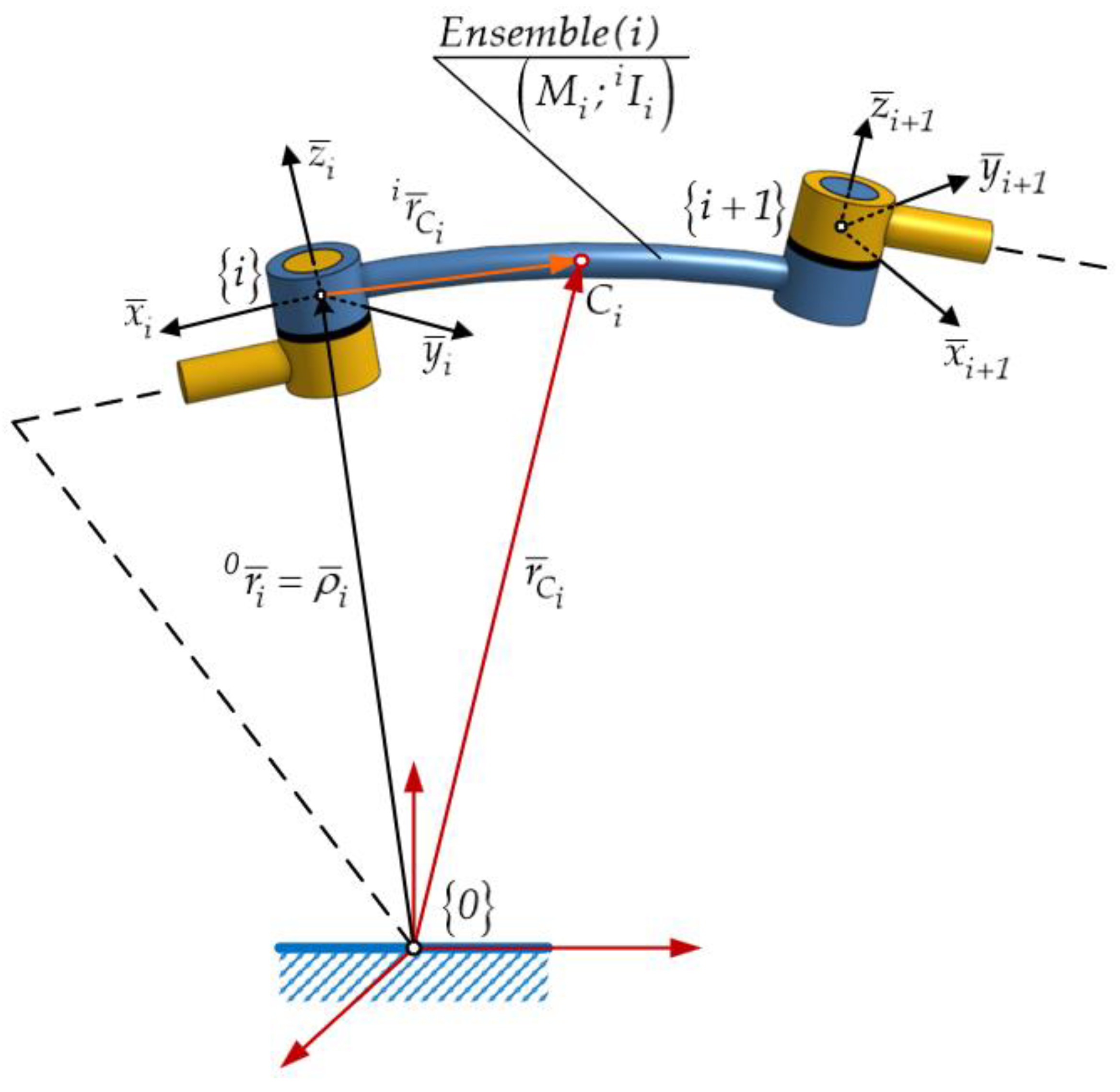
Figure 2.
Geometrical decomposition of a kinetic ensemble into a finite number of simple bodies.
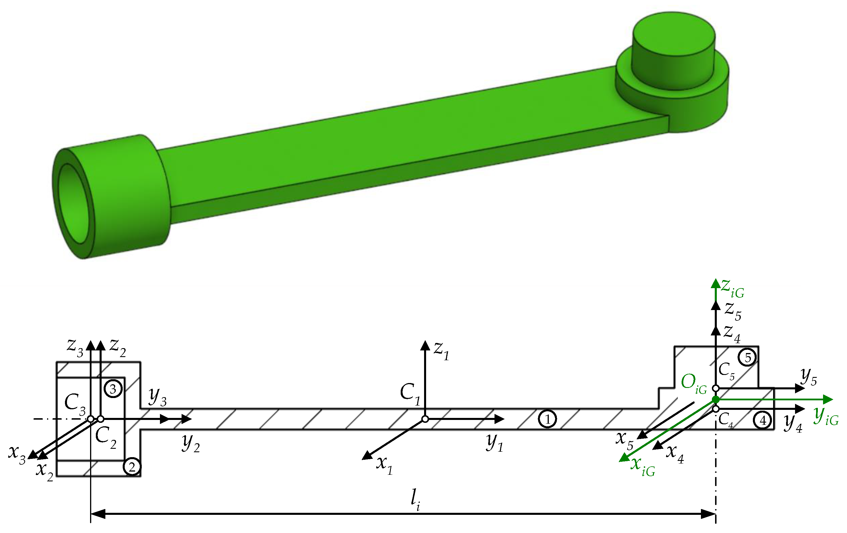
Figure 3.
Geometric Parameters Used for the Computation of Mass Distribution Properties.
Figure 4.
Distribution of the forces on a multibody system (MBS).
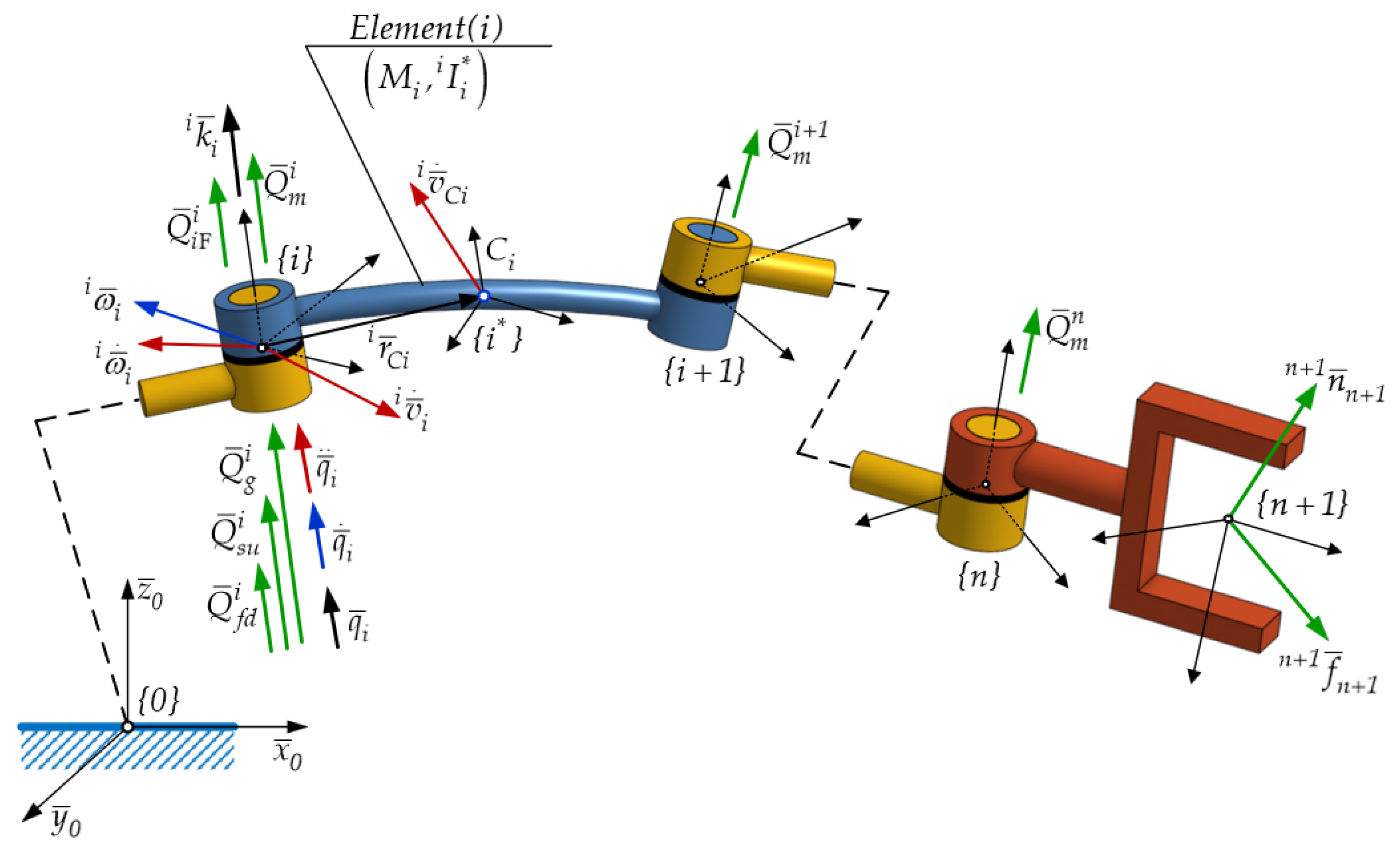
Figure 5.
The Generalized Active Forces of a multibody system (MBS).
Disclaimer/Publisher’s Note: The statements, opinions and data contained in all publications are solely those of the individual author(s) and contributor(s) and not of MDPI and/or the editor(s). MDPI and/or the editor(s) disclaim responsibility for any injury to people or property resulting from any ideas, methods, instructions or products referred to in the content. |
© 2025 by the authors. Licensee MDPI, Basel, Switzerland. This article is an open access article distributed under the terms and conditions of the Creative Commons Attribution (CC BY) license (http://creativecommons.org/licenses/by/4.0/).
Copyright: This open access article is published under a Creative Commons CC BY 4.0 license, which permit the free download, distribution, and reuse, provided that the author and preprint are cited in any reuse.


