Acceleration Energies and Higher-Order Dynamic Equations in Analytical Mechanics

1. Introduction

The study of acceleration energies and higher-order dynamic equations plays a crucial role in the field of analytical mechanics, which focuses on the mathematical and theoretical underpinnings of mechanical systems’ motion. Analytical mechanics, encompassing both Lagrangian and Hamiltonian formulations, provides a foundation for modeling complex dynamic behaviors in both rigid and multibody systems. In recent years, attention has shifted toward higher-order dynamic equations, incorporating advanced concepts such as higher-order derivatives and acceleration energies to characterize rapid and transient movements with increased accuracy [1].

The role of higher-order acceleration energies is especially significant in modern applications such as robotics and aerospace engineering, where precise control and prediction of mechanical movements are essential [2]. By expanding traditional mechanics to include these advanced energies, researchers can formulate more comprehensive equations that capture nuanced mechanical behaviors during transient motion regimes and rapid acceleration phases [3].

Based on the fundamental principles of analytical mechanics, this study investigates higher-order acceleration energies and differential principles that are indispensable for characterizing the dynamic behavior of mechanical systems.

With direct applications in robotics and mechanical engineering, the research addresses the requirements of systems that need precise control and predictive accuracy under complex motion conditions. By introducing novel formulations in advanced kinematics and dynamics, the work extends the analytical framework to encompass higher-order derivatives and acceleration energies.

This model facilitates a more comprehensive understanding of rapid and transient motion phenomena, enabling enhanced modeling accuracy for complex mechanical systems. The primary goal is to develop explicit, matrix-based representations of higher-order acceleration energies, which are essential for the modeling and control of high-velocity mechanical systems. The research focuses on integrating these advanced dynamic formulations into differential equations that effectively capture both steady-state and transitional behaviors in complex mechanical assemblies.

2. Materials and Methods

This theoretical study focuses on the advanced development of kinematic and dynamic principles in analytical mechanics, specifically concerning higher-order acceleration energies and their applications in complex mechanical systems.

The approach is based on rigorous mathematical models and matrix formulations to extend existing theories. This section outlines the theoretical framework, mathematical tools, and key equations employed in formulating higher-order dynamics for rigid and multibody systems, providing the foundation for the later analysis of dynamic behaviors under complex motion conditions.

2.1. Position and Orientation Parameters of Solid Body

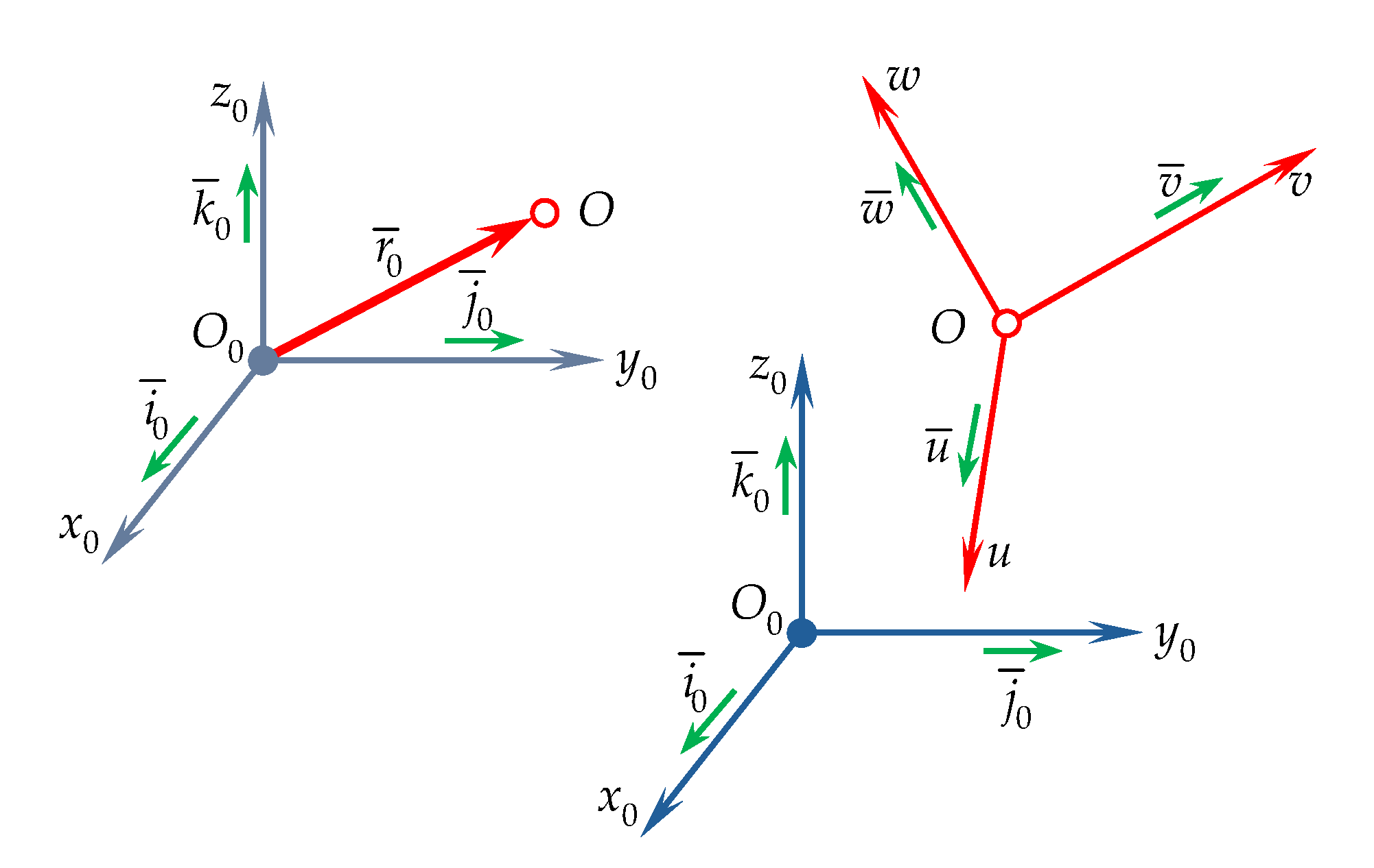
The solid body is a physical form of matter’s existence in the material universe. Consequently, the solid body is considered a material continuum. Based on this property to achieve an exact geometric solution, the solid body is decomposed into an infinite number of elementary particles, each with an infinitesimal mass and a continuous distribution throughout its geometric form. If the distances between the elementary particles are kept constant, the solid body will be characterized as a rigid solid (S). When density is consistently supported within the rigid structure, a homogeneous rigid solid is obtained. If the integration limits around the entire geometric contour are well-defined, the homogeneous body will have a simple or regular geometric shape. In this case, geometric and mass integrals are applied. Before conducting the mechanical study (static, kinematic, and dynamic modeling), it is essential to show the geometric state of the rigid body at each moment of its movement in Cartesian space. To this end, the geometric state of the simplest mechanical model, the material point, is studied first (Figure 1). Based on research from [4,5,6], the following notations are introduced:

$$\begin{array}{c}\chi =\left\{u;v;w\right\};{\chi }_0=\left\{u_0;v_0;w_0\right\},\\ where\text{\hspace{0.17em}\hspace{0.17em}\hspace{0.17em}\hspace{0.17em}}u=\left\{x;y;z\right\};v=\left\{y;z;x\right\}\ne u;w=\left\{z;x;y\right\}\ne v\end{array}$$

(1)

$$\begin{array}{c}\overline{\chi }=\left\{\overline{u};\overline{v};\overline{w}\right\};{\overline{\chi }}_0=\left\{{\overline{u}}_0;{\overline{v}}_0;{\overline{w}}_0\right\},\\ where\overline{u}=\left\{\overline{i};\overline{j};\overline{k}\right\};\overline{v}=\left\{\overline{j};\overline{k};\overline{i}\right\}\ne \overline{u};\overline{w}=\left\{\overline{k};\overline{i};\text{\hspace{0.17em}}\overline{j}\right\}\ne \overline{v}\end{array}$$

(2)

$${\delta }_{\chi }=\left\{{\alpha }_{\chi };{\beta }_{\chi };{\gamma }_{\chi }\right\};\cos {\delta }_{\chi }=c{\delta }_{\chi };\sin {\delta }_{\chi }=s{\delta }_{\chi },$$

(3)

$$O_0{x}_0{y}_0{z}_0\equiv \left\{0\right\},{O^{\prime }}_0{x^{\prime }}_0{y^{\prime }}_0{z^{\prime }}_0\equiv \left\{0^{\prime }\right\},Oxyz\equiv \left\{S\right\}.$$

(4)

In expression (1), the coordinates and axes of the Cartesian reference system are defined; in expression (2), the unit vectors (versors) of the reference system axes are specified, and in expression (3), the angles and direction cosines are defined.

Following Figure 1, the rigid body is subject to geometric study. For this purpose, two reference systems are considered: the first system, denoted as $O_0{x}_0{y}_0{z}_0=\left\{0\right\}$, is a fixed reference system, and the second system, $Oxyz=\left\{S\right\}$, is a moving reference system, permanently attached to the body, with its origin at point $O$, an arbitrary point on the rigid body. The reference system $O{x^{\prime }}_0{y^{\prime }}_0{z^{\prime }}_0=\left\{0^{\prime }\right\}$, also represented in the Figure 1, is a system with its origin at point $O$, whose orientation remains constant throughout the motion and is identical to that of the fixed reference system, $\left\{0\right\}$, meaning ${\left\{0^{\prime }\right\}}_{OR}\equiv {\left\{0\right\}}_{OR}$. The geometric state of any point belonging to the rigid body (for example, an arbitrary point $O$) represents its position, defined, according to Figure 1, by the following position vector:

$${\overline{r}}_0={\left[\begin{array}{ccc}{x}_0& y_0& z_0\end{array}\right]}^T\mathrm{relative}\mathrm{to}\mathrm{fixed}\mathrm{system}\left\{0\right\}.$$

(5)

For a free material point, the three linear coordinates defined in (5) are independent and represent the degrees of freedom (d.o.f.). The study then extends to a vector or an axis belonging to the Cartesian reference system (Figure 1).

This geometric state is referred to as orientation (angular state). Orientation (angular state) is defined by using unit vectors. For any unit vector $\overline{\chi }\in \left\{S\right\}$, assumed to be known in relation to one of the reference systems $\left\{0\right\}$or$\left\{0^{\prime }\right\}$, the orientation will be defined by means of the direction cosines.

$$\overline{\chi }={\overline{\chi }}^T\cdot \left(\begin{array}{l}{\overline{i}}_0\\ {\overline{j}}_0\\ {\overline{k}}_0\end{array}\right)=\left(\begin{array}{l}c{\alpha }_{\chi }\\ c{\beta }_{\chi }\\ c{\gamma }_{\chi }\end{array}\right)\equiv {\left(\begin{array}{l}c\alpha \\ c\beta \\ c\gamma \end{array}\right)}_{\chi }\mathrm{where}{\overline{\chi }}^T\cdot \overline{\chi }=c^2{\alpha }_{\chi }+c^2{\beta }_{\chi }+c^2{\gamma }_{\chi }=1.$$

(6)

In accordance with linear algebra, the symbol ${\overline{\chi }}^T$ in expression (6) defines the transpose of the matrix. Considering the second expression in (6), it can be observed that the orientation of any vector or axis is defined by two independent angles. The geometric aspects presented earlier are examined in the context of an orthogonal, right-handed reference system (see Figure 1, $Ouvw\equiv Oxyz\equiv \left\{S\right\}$) relative to the fixed reference system $\left\{0\right\}$. In this case, the geometric state is represented by position and orientation. Position is defined by expression (5), while orientation is defined by the rotation matrix [4,6,7]:

$${}_S{}^0\left[R\right]=\left[\begin{array}{ccc}\overline{i}& \overline{j}& \overline{k}\end{array}\right]=\left[\begin{array}{ccc}{\left(\begin{array}{l}c\alpha \\ c\beta \\ c\gamma \end{array}\right)}_x& {\left(\begin{array}{l}c\alpha \\ c\beta \\ c\gamma \end{array}\right)}_y& {\left(\begin{array}{l}c\alpha \\ c\beta \\ c\gamma \end{array}\right)}_z\end{array}\right].$$

(7)

The resulting rotation matrix defined by (7) contains the unit vectors of the reference system $\left\{S\right\}$ relative to the fixed reference system$\left\{0\right\}$. The rotation matrix, or direction cosine matrix, describes the orientation of each axis of the moving reference system attached to the rigid body in relation to a fixed reference system. Among the nine direction cosines in the rotation matrix, six mathematical relationships can be proved. Therefore, the orientation of a moving reference system relative to a fixed reference system can be defined by a maximum of three independent parameters, represented by the orientation angles. Consequently, the resulting orientation of a reference system $\left\{S\right\}$relative to another reference system, $\left\{0\right\}$or$\left\{0^{\prime }\right\}$, can be defined by three independent orientation angles (degrees of freedom), according to [4,6]:

$$\underset{\left(3x1\right)}{\overline{\overline{\psi }}\left(t\right)}={\left[\begin{array}{ccc}{\alpha }_u\left(t\right)& {\beta }_v\left(t\right)& {\gamma }_w\left(t\right)\end{array}\right]}^T.$$

(8)

The angles included in (8) are components of the orientation column matrix $\overline{\overline{\psi }}\left(t\right)$, which geometrically describe dihedral angles between two geometric planes:

$${\chi }_0=\left\{u_0;v_0;w_0\right\}=cst.\to fixedplane\in \left\{0^{\prime }\right\}/\left\{0\right\}.$$

(9)

$$\chi =\left\{u;v;w\right\}=cst.\to mobileplane\in \left\{S\right\}$$

(10)

Physically, the three angles defined by expression (9) represent a simple rotation around one of the three axes of the Cartesian reference system: $\chi =\left\{u;v;w\right\}$.

Based on the research in [4,6], combining these three simple rotations results in 12 sets of orientation angles (8). Considering $\chi =\left\{x;y;z\right\}$, the expressions for the three simple rotation matrices are further developed as follows:

$$R\left(\overline{\chi };{\delta }_{\chi }\right)=\left\{R\left(\overline{x};{\alpha }_x\right);R\left(\overline{y};{\beta }_y\right);\text{\hspace{0.17em}\hspace{0.17em}}R\left(\overline{z};{\gamma }_z\right)\right\}.$$

(11)

The following mathematical representation of the generalized rotation matrix is proposed:

$$\begin{array}{l}R\left(\overline{\chi };{\delta }_{\chi }\right)=\left\{R\left(\overline{x};{\alpha }_x\right);R\left(\overline{y};{\beta }_y\right);\text{\hspace{0.17em}\hspace{0.17em}}R\left(\overline{z};{\gamma }_z\right)\right\}=\\ =\left[\begin{array}{ccc}c\left({\delta }_{\chi }\cdot {\Delta }_{yz}\right)& -s\left({\delta }_{\chi }\cdot {\Delta }_z\right)& s\left({\delta }_{\chi }\cdot {\Delta }_y\right)\\ s\left({\delta }_{\chi }\cdot {\Delta }_z\right)& c\left({\delta }_{\chi }\cdot {\Delta }_{zx}\right)& -s\left({\delta }_{\chi }\cdot {\Delta }_x\right)\\ -s\left({\delta }_{\chi }\cdot {\Delta }_y\right)& s\left({\delta }_{\chi }\cdot {\Delta }_x\right)& c\left({\delta }_{\chi }\cdot {\Delta }_{xy}\right)\end{array}\right]\end{array}$$

(12)

where,

$$\begin{array}{c}\underset{\left\{\chi =\left\{u;v\right\}\right\}}{{\Delta }_{uv}}=\left\{{\Delta }_{yz};{\Delta }_{zx};{\Delta }_{xy}\right\}=\\ =\left\{\left(\begin{array}{l}1\\ 0\end{array}\right),if{\delta }_{\chi }=\left\{\left\{\begin{array}{c}\left({\beta }_y;{\gamma }_z\right)\\ {\alpha }_x\end{array}\right\};\left\{\begin{array}{c}\left({\gamma }_z;{\alpha }_x\right)\\ {\beta }_y\end{array}\right\};\left\{\begin{array}{c}\left({\alpha }_x;{\beta }_y\right)\\ {\gamma }_z\end{array}\right\}\right\}\right\}\end{array}$$

(13)

and,

$$\underset{\left\{\chi =u\right\}}{{\Delta }_u}=\left\{{\Delta }_x;{\Delta }_y;{\Delta }_z\right\}=1-\underset{\left\{\chi =\left\{v;w\right\}\right\}}{{\Delta }_{vw}.}$$

(14)

By substituting (13) and (14) into the generalized expression (12), the simple rotation matrices defined in (11) are obtained. The generalized matrix can thus be written as follows:

$$R\left(\overline{\chi };{\delta }_{\chi }\right)=Diag\left[{\overline{\overline{\Delta }}}_{uv}\right]+\left[{\overline{\overline{\Delta }}}_u\times \right],$$

(15)

$$\underset{\left(3\times 1\right)}{{\overline{\overline{\Delta }}}_{uv}}={\left[c\left({\delta }_{\chi }\cdot {\Delta }_{yz}\right)c\left({\delta }_{\chi }\cdot {\Delta }_{zx}\right)c\left({\delta }_{\chi }\cdot {\Delta }_{xy}\right)\right]}^T,$$

(16)

$$\underset{\left(3\times 1\right)}{{\overline{\overline{\Delta }}}_u}={\left[s\left({\delta }_{\chi }\cdot {\Delta }_x\right)s\left({\delta }_{\chi }\cdot {\Delta }_y\right)s\left({\delta }_{\chi }\cdot {\Delta }_z\right)\right]}^T.$$

(17)

In expression (15), the symbol $\left[{\overline{\overline{\Delta }}}_u\times \right]$defines the antisymmetric matrix associated with vector (17), while $Diag\left[{\overline{\overline{\Delta }}}_{uv}\right]$represents the diagonal matrix, determined as:

$$\underset{\left(3x3\right)}{Diag\left({\overline{\overline{\Delta }}}_{uv}\right)}=\left[\begin{array}{ccc}c\left({\delta }_{\chi }\cdot {\Delta }_{yz}\right)& 0& 0\\ 0& c\left({\delta }_{\chi }\cdot {\Delta }_{zx}\right)& 0\\ 0& 0& c\left({\delta }_{\chi }\cdot {\Delta }_{xy}\right)\end{array}\right].$$

(18)

The matrix (15) can also be defined by means of the following classical formulation:

$$R\left(\overline{\chi };{\delta }_{\chi }\right)=\overline{\chi }\cdot {\overline{\chi }}^T\cdot \left(1-c{\delta }_{\chi }\right)+I_3\cdot c{\delta }_{\chi }+\left(\overline{\chi }\times s{\delta }_{\chi }\right).$$

(19)

According to the research [4,5,8], the three simple rotations defined by (8) can be performed either around the fixed axes or the moving axes, belonging to the $\left\{S\right\}$ and $\left\{0^{\prime }\right\}$/$\left\{0\right\}$reference systems. The resulting rotation matrix, denoted ${}_S{}^0\left[R\right]$, which expresses the orientation of the $\left\{S\right\}$reference system relative to $\left\{0\right\}$ fixed reference system, is defined by expressions that also include matrix exponentials, as follows:

$${}_S{}^0\left[R\right]=R\left(\overline{u};{\alpha }_u\right)\cdot R\left(\overline{v};{\beta }_v\right)\cdot \text{\hspace{0.17em}}R\left(\overline{w};{\gamma }_w\right),$$

(20)

$${}_S{}^0\left[R\right]={\displaystyle \prod _{\left\{\overline{\chi };{\delta }_{\chi }\right\}}R\left(\overline{\chi };{\delta }_{\chi }\right)}={\displaystyle \prod _{\left\{\chi =\left\{u;v;w\right\}\right\}}\exp }\left[\overline{\chi }\times {\delta }_{\chi }\right]={\displaystyle \prod _{\left\{u;v\right\}}\left\{I_3\cdot {\overline{\overline{\Delta }}}_{uv}+\left[{\overline{\overline{\Delta }}}_u\right]\right\}}.$$

(21)

Using the author’s research on matrix exponentials [5,9,10], the resulting rotation matrix can be expressed in a new form as follows:

$$\left\{\begin{array}{c}{}_S{}^0\left[R\right]={\displaystyle \prod _{\left\{\overline{\chi };{\delta }_{\chi }\right\}}R\left(\overline{\chi };{\delta }_{\chi }\right)}={\displaystyle \prod _{\left\{\chi =\left\{u;v;w\right\}\right\}}\exp }\left[\overline{\chi }\times {\delta }_{\chi }\right]=\\ =\exp \left[\overline{u}\times {\alpha }_u\right]\cdot \exp \left[\overline{v}\times {\beta }_v\right]\cdot \exp \left[\overline{w}\times {\gamma }_w\right]\end{array}\right\}.$$

(22)

Expressions (5) and (8), presented above, define the position and orientation of a right-handed reference system. These mathematical expressions will be generalized for the case of a rigid body. According to [5,6], a rigid body is composed of an infinite number of material particles and an infinite number of geometric axes, parallel and perpendicular to each other, characterized by a continuous distribution throughout the entire volume of the rigid body [5,8]. The rigid body also includes an infinite number of sets consisting of three orthogonal geometric planes, continuously distributed throughout its volume. 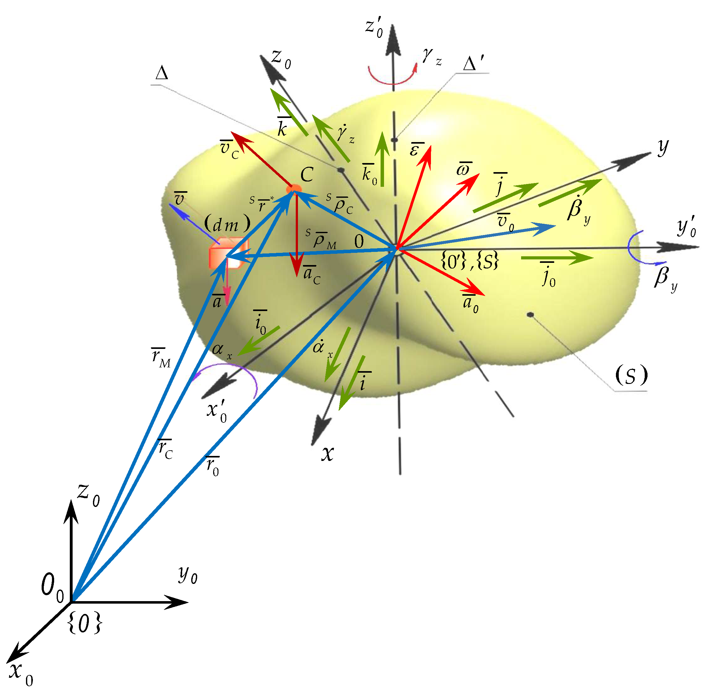Geometrically, to define a right-handed reference system with its origin at an arbitrary point $O$belonging to the rigid body, it is sufficient to select a single set composed of three orthogonal planes. According to expression (4) and Figure 2, this reference system is denoted $Oxyz\equiv \left\{S\right\}$. The reference system $\left\{S\right\}$is attached to the rigid body. Expressions (5) and (8) define the position and orientation of this system.

Since the purpose of this paper is to study advanced dynamics, two material points belonging to the rigid body are considered, satisfying the conditions $M\ne O$ and $C\ne \left\{O;M\right\}$. The expressions defining the absolute position become time-dependent vector functions [4,11], as follows:

$${\overline{r}}_M\left(t\right)={\overline{r}}_0\left(t\right)+{\overline{\rho }}_M\left(t\right)={\overline{r}}_0\left(t\right)+{}_S{}^0\left[R\right]\left(t\right)\cdot {}^S\overline{\rho }_M,$$

(23)

$${\overline{r}}_C\left(t\right)={\overline{r}}_0\left(t\right)+{\overline{\rho }}_C\left(t\right)={\overline{r}}_0\left(t\right)+{}_S{}^0\left[R\right]\left(t\right)\cdot {}^S\overline{\rho }_C,$$

(24)

$$\mathrm{where}{\overline{\rho }}_M\left(t\right)\ne {\overline{\rho }}_C\left(t\right)\mathrm{and}{\overline{r}}_M\left(t\right)\ne {\overline{r}}_C\left(t\right).$$

(25)

Considering expressions (23) and (25), the absolute position equation can be written using matrix exponentials [6,9,10], as follows:

$$\left\{\begin{array}{c}{\overline{r}}_M\left(t\right)={\overline{r}}_0\left(t\right)+{\displaystyle \prod _{\left\{\chi =\left\{u;v;w\right\}\right\}}\exp }\left[\overline{\chi }\times {\delta }_{\chi }\right]\cdot {}^S\overline{\rho }_M=\\ ={\overline{r}}_0\left(t\right)+\left\{\exp \left[\overline{u}\times {\alpha }_u\right]\cdot \exp \left[\overline{v}\times {\beta }_v\right]\cdot \exp \left[\overline{w}\times {\gamma }_w\right]\right\}\cdot {{}^S\overline{\rho }}_M\end{array}\right\}.$$

(26)

The absolute position equation for any material point belonging to the rigid body can be determined when the position ${\overline{r}}_0\left(t\right)$ and the orientation ${}_S{}^0\left[R\right]\left(t\right)$ of the moving system $Oxyz\equiv \left\{S\right\}$ are known. Analyzing expressions (23) and (24) reveals that the orientation is invariant for all points of the rigid body. Based on these geometric considerations, the body is represented by the reference system $Oxyz\equiv \left\{S\right\}$. This system is geometrically defined by six independent parameters or degrees of freedom, included in the symbol:

$$\underset{\left(6\times 1\right)}{\overline{\overline{X}}}\left(t\right)=\left[\begin{array}{c}\overline{r}_0\left(t\right)\\ \overline{\overline{\psi }}t\end{array}\right]=\left[\begin{array}{c}{\left[\begin{array}{ccc}{x}_0\left(t\right)& y_0\left(t\right)& z_0\left(t\right)\end{array}\right]}^T\\ {\left[\begin{array}{ccc}{\alpha }_u\left(t\right)& {\beta }_v\left(t\right)& {\gamma }_w\left(t\right)\end{array}\right]}^T\end{array}\right]=\left[\begin{array}{c}{q}_i\left(t\right)\cdot {\delta }_i,i=1\to 6\end{array}\right].$$

(27)

where ${\delta }_i=\left\{\left(1-{\Delta }_i\right),if{q}_i-linear,{\Delta }_i,if{q}_i-angular\right\}$and $q_j\left(t\right)$is the generalized coordinate, ${\Delta }_i=\left\{\left(1,q_i-angular\right),\left(0,q_i-linear\right)\right\}$is an operator that highlights the type of degrees of freedom:

$$\begin{array}{c}\left\{\overline{\theta }\left(t\right);\dot{\overline{\theta }}\left(t\right);\ddot{\overline{\theta }}\left(t\right);\cdots ;\stackrel{\left(m\right)}{\overline{\theta }}\left(t\right)\right\}=\\ =\left\{q_i\left(t\right);{\dot{q}}_i\left(t\right);{\ddot{q}}_i\left(t\right);\cdots ;\stackrel{\left(m\right)}{q_i}\left(t\right),i=1\to 6,m\ge 1\right\}\end{array}$$

(28)

The symbols presented in expression (28) define higher-order generalized variables in the case of rapid motions, where $m\ge 1$ is the order of the time derivative.

In advanced mechanics, instead of expression (8), the following definition is used for the angular orientation vector:

$$\overline{\psi }\left(t\right)={}^{0}J{}_{\psi }\left[{\alpha }_u\left(t\right)-{\beta }_v\left(t\right)-{\gamma }_w\left(t\right)\right]\cdot \overline{\overline{\psi }}\left(t\right)=\overline{\psi }\left[q_j\left(t\right)\cdot {\Delta }_j;j=1\to k^{\ast }\right]$$

(29)

where ${{}^{0}J}_{\psi }$ is the angular transfer matrix, which is a $\left(3\times 3\right)$ matrix defined as a function of the orientation angles, and specified according to the expression below:

$${}^{0}J{}_{\psi }\left[{\alpha }_u\left(t\right)-{\beta }_v\left(t\right)-{\gamma }_w\left(t\right)\right]=\left[\begin{array}{ccc}\overline{u}& R\left(\overline{u};{\alpha }_u\right)\cdot \overline{v}& R\left(\overline{u};{\alpha }_u\right)\cdot R\left(\overline{v};{\beta }_v\right)\cdot \overline{w}\end{array}\right]$$

(30)

The position and orientation of the $Oxyz\equiv \left\{S\right\}$moving reference system, relative to any other system, such as the $\left\{0\right\}$ fixed reference system can be represented in matrix form using transformations based on matrix exponentials:

$$\underset{\left(4\times 4\right)}{{}_S{}^0\left[T\right]}\left(t\right)=\left[\begin{array}{cc}{}_S{}^0\left[R\right]\left(t\right)& \overline{p}\left(t\right)\\ \begin{array}{ccc}0& 0& 0\end{array}& 1\end{array}\right]=\left[\begin{array}{cc}{\displaystyle \prod _{\left\{\chi =\left\{u;v;w\right\}\right\}}\exp }\left[\overline{\chi }\times {\delta }_{\chi }\right]& \overline{p}\left(t\right)\\ \begin{array}{ccc}0& 0& 0\end{array}& 1\end{array}\right],$$

(31)

$$\overline{p}\left(t\right)={\displaystyle \sum _{\left\{\chi =\left\{u;v;w\right\}\right\}}\left\{{\displaystyle \prod _{\left\{\chi =\left\{u;v;w\right\}\right\}}\exp }\left[\overline{\chi }\times {\delta }_{\chi }\right]\right\}}\cdot {\overline{b}}_{\chi }+\left\{{\displaystyle \prod _{\left\{\chi =\left\{u;v;w\right\}\right\}}\exp }\left[\overline{\chi }\times {\delta }_{\chi }\right]\right\}\cdot {\overline{p}}^{\left(0\right)}\cdot {\Delta }_p$$

(32)

$$\mathrm{where}{\Delta }_p=\left\{\left\{0;\overline{p}={\overline{r}}_0\right\};\left\{1;\overline{p}={\overline{r}}_M\right\}\right\},$$

(33)

$$\mathrm{and}{\overline{b}}_{\chi }=\left[{\overline{\chi }}^{\left(0\right)}\cdot {\overline{\chi }}^{\left(0\right)T}\cdot \left({\delta }_{\chi }-s{\delta }_{\chi }\right)+\right.I_3\cdot s{\delta }_{\chi }\left.+\left({\overline{\chi }}^{\left(0\right)}\times \right)\cdot \left(1-c{\delta }_{\chi }\right)\right]\cdot \left[{\overline{p}}^{\left(0\right)}\times {\overline{\chi }}^{\left(0\right)}\cdot {\Delta }_{\chi }\right].$$

(34)

Expression (32) defines the position vector of the $\left\{S\right\}$ moving system relative to the fixed system $\left\{0\right\}$, while (34) represents a vector defined as a function of screw parameters (homogeneous coordinates).

The conclusion and defining expressions presented in this introductory section will be applied further in the study of advanced kinematics and dynamics of mechanical systems.

2.2. The Parameters of Advanced Mechanics

Based on the authors’ research, this chapter will present a series of new formulations about advanced kinematic concepts. A rigid body (S) represented in Figure 2 and undergoing general motion is considered. By applying the first-order absolute derivative to the parametric motion equations, we obtain:

$${\dot{\overline{r}}}_M\left(t\right)={\dot{\overline{r}}}_0\left(t\right)+{\dot{\overline{\rho }}}_M\left(t\right)={\dot{\overline{r}}}_0\left(t\right)+{}_S{}^0\left[\dot{R}\right]\left(t\right)\cdot {}_S{}^0\left[R\right]{}^T\left(t\right)\cdot {}_S{}^0\left[R\right]\left(t\right)\cdot {{}^S\overline{\rho }}_M.$$

(35)

According to [12,13,14,15,16,17], the antisymmetric matrix associated to angular vector is:

$${}_S{}^0\left[\dot{R}\right]\left(t\right)\cdot {}_S{}^0\left[R\right]{}^T\left(t\right)=\left(\overline{\omega }\times \right)=\left[\begin{array}{ccc}0& -{\omega }_z& {\omega }_y\\ {\omega }_z& 0& -{\omega }_x\\ -{\omega }_y& {\omega }_x& 0\end{array}\right].$$

(36)

Finally, expressions for linear velocities and accelerations are obtained in the form:

$${\overline{a}}_M={\overline{a}}_0+\overline{\epsilon }\times {\overline{\rho }}_M+\overline{\omega }\times \overline{\omega }\times {\overline{\rho }}_M,{\overline{v}}_M={\overline{v}}_0+\overline{\omega }\times {\overline{\rho }}_M.$$

(37)

The absolute position equation, expressed in terms of matrix exponentials results:

$${\overline{r}}_M\left(t\right)={\overline{r}}_0\left(t\right)+\exp \left[{\displaystyle \sum _{\chi =\left\{u,v,w\right\}}\overline{\chi }\times {\delta }_{\chi }}\right]{}^S\overline{\rho }{}_M={\overline{r}}_0\left(t\right)+\exp \left\{\overline{u}\times {\alpha }_u+\overline{v}\times {\beta }_v+\overline{w}\times {\gamma }_w\right\}\cdot {}^S\overline{\rho }{}_M.$$

(38)

In advanced kinematics and dynamics, the higher-order derivatives applied to position vectors and rotation matrices are expressed as follows:

$$\stackrel{\left(k-1\right)}{{\overline{v}}_M}={\displaystyle \frac{d^k{\overline{r}}_M\left(t\right)}{d{t}^k}}={\displaystyle \sum _{j=1}^6\left[\frac{\partial \stackrel{\left(m\right)}{{\overline{r}}_M}}{\partial \stackrel{\left(m\right)}{q_j}}\cdot \stackrel{\left(k\right)}{q_j}\right]}+{\displaystyle \sum _{j=1}^6{\displaystyle \sum _{r=1}^{k-1}\left\{\frac{{\displaystyle \prod _{p=1}^r\left(k-p\right)}}{p!}\cdot \left[\frac{p!\cdot m!}{\left(m+p\right)!}\cdot \frac{\partial \stackrel{\left(m+p\right)}{{\overline{r}}_M}}{\partial \stackrel{\left(m\right)}{q_j}}\cdot \stackrel{\left(k-p\right)}{q_j}\right]\right\}}},$$

(39)

$$\begin{array}{c}{\displaystyle \frac{d^k}{d{t}^k}}\left\{{}_S{}^0\left[R\right]\left(t\right)\right\}={}_S{}^0\left[R\right]\left[\stackrel{\left(k\right)}{q_j}\cdot {\Delta }_j\right]={\displaystyle \sum _{j=1}^i\left\{\frac{\partial }{\partial \stackrel{\left(m\right)}{q_j}}\left\{\stackrel{\left(m\right)}{{}_S{}^0\left[R\right]}\right\}\cdot \stackrel{\left(k\right)}{q_j}\cdot {\Delta }_j\right\}}+\\ +{\displaystyle \sum _{j=1}^6{\displaystyle \sum _{r=1}^{k-1}\left\{\frac{{\displaystyle \prod _{p=1}^r\left(k-p\right)}}{p!}\cdot \frac{d^p}{d{t}^p}\left\{\frac{\partial }{\partial \stackrel{\left(m\right)}{q_j}}\left\{\stackrel{\left(m\right)}{{}_S{}^0\left[R\right]}\right\}\right\}\cdot \stackrel{\left(k-p\right)}{q_j}\cdot {\Delta }_j\right\}}}=\\ ={\displaystyle \sum _{j=1}^6\left\{\frac{\partial }{\partial \stackrel{\left(m\right)}{q_j}}\left\{\stackrel{\left(m\right)}{{}_S{}^0\left[R\right]}\right\}\cdot \stackrel{\left(k\right)}{q_j}\cdot {\Delta }_j\right\}}+{\displaystyle \sum _{j=1}^6{\displaystyle \sum _{r=1}^{k-1}\left\{\frac{{\displaystyle \prod _{p=1}^r\left(k-p\right)}}{p!}\cdot \left\{\frac{p!\cdot m!}{\left(m+p\right)!}\cdot \frac{\partial }{\partial \stackrel{\left(m\right)}{q_j}}\left\{\stackrel{\left(m+p\right)}{{}_S{}^0\left[R\right]}\right\}\right\}\cdot \stackrel{\left(k-p\right)}{q_j}\cdot {\Delta }_j\right\}}}\end{array}$$

(40)

$$wherek\ge 1;k=\left\{1;2;3;4;5;\mathrm{.....}\right\},andm\ge \left(k+1\right);m=\left\{2;3;4;5;\mathrm{.....}\right\}$$

The defining expressions for angular velocities and accelerations can be proved based on matrix exponentials, as follows:

$$\left\{\begin{array}{c}\overline{\omega }\left[{\alpha }_u\left(t\right)-{\beta }_v\left(t\right)-{\gamma }_w\left(t\right)\right]={\dot{\alpha }}_u\left(t\right)\cdot \left\{\exp \left[0\right]\right\}\cdot {\overline{u}}^{\left(0\right)}+\\ +{\dot{\beta }}_v\left(t\right)\cdot \left\{\exp \left[\overline{u}\left(t\right)\times {\alpha }_u\left(t\right)\right]\right\}\cdot {\overline{v}}^{\left(0\right)}+\\ +\left.{\dot{\gamma }}_w\left(t\right)\cdot \left\{\exp \left[\overline{u}\left(t\right)\times {\alpha }_u\left(t\right)\right]\cdot \exp \left[\overline{v}\left(t\right)\times {\beta }_v\left(t\right)\right]\right\}\cdot {\overline{w}}^{\left(0\right)}\right\}\end{array}\right\},$$

(41)

$$\left\{\begin{array}{c}\stackrel{\left(m\right)}{\overline{\omega }}\left[{\alpha }_u\left(t\right)-{\beta }_v\left(t\right)-{\gamma }_w\left(t\right)\right]={\displaystyle \frac{d^k}{d{t}^k}}\left\{{\dot{\alpha }}_u\left(t\right)\cdot \left\{\exp \left[0\right]\right\}\cdot {\overline{u}}^{\left(0\right)}\right\}+\\ +{\displaystyle \frac{d^k}{d{t}^k}}\left\{{\dot{\beta }}_v\left(t\right)\cdot \left\{\exp \left[\overline{u}\left(t\right)\times {\alpha }_u\left(t\right)\right]\right\}\cdot {\overline{v}}^{\left(0\right)}\right\}+\\ +\left.{\displaystyle \frac{d^k}{d{t}^k}}\left\{{\dot{\gamma }}_w\left(t\right)\cdot \left\{\exp \left[\overline{u}\left(t\right)\times {\alpha }_u\left(t\right)\right]\cdot \exp \left[\overline{v}\left(t\right)\times {\beta }_v\left(t\right)\right]\right\}\cdot {\overline{w}}^{\left(0\right)}\right\}\right\}\end{array}\right\}.$$

(42)

Although the use of matrix exponentials may appear complex, it offers advantages, including the elimination of reference systems, which can impose certain restrictions.

This is evident in the previously presented equations by ${\overline{\chi }}^{\left(0\right)}=\left\{{\overline{u}}^{\left(0\right)};{\overline{v}}^{\left(0\right)};{\overline{w}}^{\left(0\right)}\right\}$, showing that the unit vectors correspond to the initial state of the reference system $Oxyz\equiv \left\{S\right\}$. The position of the center of mass is found relative to the reference system $O_0{x^{\prime }}_0{y^{\prime }}_0{z^{\prime }}_0\equiv \left\{0^{\prime }\right\}$, as:

$${\overline{\rho }}_C\left(t\right)={\displaystyle \frac{{\displaystyle \int {\overline{\rho }}_M\left(t\right)\cdot dm}}{{\displaystyle \int dm}}}={\displaystyle \frac{{\displaystyle \int {\overline{\rho }}_M\left(t\right)\cdot dm}}{M}}={}_S{}^0\left[R\right]\left(t\right)\cdot {}^S\overline{\rho }{}_C.$$

(43)

The position of the mass center relative to $O_0{x}_0{y}_0{z}_0\equiv \left\{0\right\}$ reference system at first, in classical form and then in an exponential form, is presented:

$$\begin{array}{c}{\overline{r}}_C\left(t\right)={\displaystyle \frac{{\displaystyle \int {\overline{r}}_M\left(t\right)\cdot dm}}{M}}={\overline{r}}_0\left(t\right)+{\overline{\rho }}_C\left(t\right)={\overline{r}}_0\left(t\right)+\exp \left[{\displaystyle \prod _{\left\{\chi =\left\{u;v;w\right\}\right\}}\exp }\left[\overline{\chi }\times {\delta }_{\chi }\right]\right]\cdot {}^S\overline{\rho }{}_C=\\ ={\overline{r}}_0\left(t\right)+\left\{\exp \left[\overline{u}\times {\alpha }_u\right]\cdot \exp \left[\overline{v}\times {\beta }_v\right]\cdot \exp \left[\overline{w}\times {\gamma }_w\right]\right\}\cdot {}^S\overline{\rho }{}_C.\end{array}$$

(44)

If first and second-order derivatives with respect to time are applied to expression (44) the linear velocity and acceleration of the center of mass are ultimately obtained:

$$\begin{array}{c}{\overline{v}}_C\left(t\right)={\dot{\overline{r}}}_C\left(t\right)={\dot{\overline{r}}}_0\left(t\right)+{\dot{\overline{\rho }}}_C\left(t\right)={\dot{\overline{r}}}_0\left(t\right)+{}_S{}^0\left[\dot{R}\right]\left(t\right)\cdot {}_S{}^0\left[R\right]{}^T\left(t\right)\cdot {}_S{}^0\left[R\right]\left(t\right)\cdot {}^S\overline{\rho }{}_C=\\ ={\overline{v}}_0\left(t\right)+\overline{\omega }\left(t\right)\times {\overline{\rho }}_C\left(t\right)={\displaystyle \frac{d}{dt}}\left\{{\overline{r}}_0\left(t\right)+\left\{\exp \left[{\displaystyle \prod _{\left\{\chi =\left\{u;v;w\right\}\right\}}\exp }\left[\overline{\chi }\times {\delta }_{\chi }\right]\right]\right\}\cdot {{}^S\overline{\rho }}_C\right\}=\\ ={\displaystyle \frac{d}{dt}}\left\{{\overline{r}}_0\left(t\right)+\left\{\exp \left[\overline{u}\times {\alpha }_u\right]\cdot \exp \left[\overline{v}\times {\beta }_v\right]\cdot \exp \left[\overline{w}\times {\gamma }_w\right]\right\}\cdot {{}^S\overline{\rho }}_C\right\}.\end{array}$$

(45)

$${\overline{a}}_C={\dot{\overline{v}}}_C\left(t\right)={\dot{\overline{v}}}_0\left(t\right)+{\displaystyle \frac{d}{dt}}\left[\overline{\omega }\left(t\right)\times {\overline{\rho }}_C\left(t\right)\right]={\overline{a}}_0+\overline{\epsilon }\times {\overline{\rho }}_C+\overline{\omega }\times \overline{\omega }\times {\overline{\rho }}_C.$$

(46)

The absolute linear accelerations of higher orders, with respect to mass center, are:

$$\stackrel{\left(k\right)}{{\overline{v}}_C}\left(t\right)={\displaystyle \frac{d^{k+1}}{d{t}^{k+1}}}\left\{{\overline{r}}_0\left(t\right)+{}_S{}^0\left[R\right]\left(t\right)\cdot {{}^S\overline{\rho }}_C\right\}=\stackrel{\left(k\right)}{{\overline{v}}_0}\left(t\right)+{\displaystyle \frac{d^k}{d{t}^k}}\left[\overline{\omega }\left(t\right)\times {\overline{\rho }}_C\right]$$

(47)

$$\begin{array}{c}\stackrel{\left(k\right)}{{\overline{v}}_C}\left(t\right)={\displaystyle \frac{d^{k+1}}{d{t}^{k+1}}}\left\{{\overline{r}}_0\left(t\right)+{}_S{}^0\left[R\right]\left(t\right)\cdot {{}^S\overline{\rho }}_C\right\}=\stackrel{\left(k\right)}{{\overline{v}}_0}\left(t\right)+{\displaystyle \frac{d^k}{d{t}^k}}\left[\overline{\omega }\left(t\right)\times {\overline{\rho }}_C\right]=\\ ={\displaystyle \frac{d^{k+1}}{d{t}^{k+1}}}\left\{{\overline{r}}_0\left(t\right)+\exp \left[{\displaystyle \sum _{\chi =\left\{u,v,w\right\}}\left[\overline{\chi }\times {\delta }_{\chi }\right]}\right]\cdot {{}^S\overline{\rho }}_C\right\}=\\ ={\displaystyle \frac{d^{k+1}}{d{t}^{k+1}}}\left\{{\overline{r}}_0\left(t\right)+\left\{\exp \left[\overline{u}\times {\alpha }_u+\overline{v}\times {\beta }_v+\overline{w}\times {\gamma }_w\right]\cdot {{}^S\overline{\rho }}_C\right\}\right\}\end{array}$$

(48)

In dynamic modeling, the following expression is applied:

$$\left\{\begin{array}{c}{\displaystyle \frac{d}{dt}}\left({\overline{\rho }}_M\left(t\right)\right)={\displaystyle \frac{d}{dt}}\left({\overline{\rho }}_C\left(t\right)+{\overline{r}}^{\ast }\left(t\right)\right)={\displaystyle \frac{d}{dt}}\left({}_S{}^0\left[R\right]\left(t\right)\cdot \left({}^S\overline{\rho }{}_C+{{}^S\overline{r}}^{\ast }\right)\right)=\\ =\overline{\omega }\left(t\right)\times {\overline{\rho }}_M\left(t\right)=\overline{\omega }\left(t\right)\times {\overline{\rho }}_C\left(t\right)+\overline{\omega }\left(t\right)\times {\overline{r}}^{\ast }\left(t\right).\end{array}\right\}.$$

(49)

Using the author’s research [10,11,13] on time functions for position and orientation, the following differential properties have been developed in the study of advanced kinematics and dynamics of the rigid body, according to the expressions:

$${\displaystyle \frac{\partial {\overline{r}}_C}{\partial q_j}}={\displaystyle \frac{\partial {\overline{v}}_C}{\partial {\dot{q}}_j}}={\displaystyle \frac{\partial {\overline{a}}_C}{\partial {\ddot{q}}_j}}={\displaystyle \frac{\partial {\dot{\overline{a}}}_C}{\partial {\stackrel{⃛}{q}}_j}}={\displaystyle \frac{\partial {\ddot{\overline{a}}}_C}{\partial {\stackrel{⃜}{q}}_j}}=\mathrm{...}\equiv {\displaystyle \frac{\partial \stackrel{\left(m\right)}{{\overline{r}}_C}}{\partial \stackrel{\left(m\right)}{q_j}}},$$

(50)

$${\displaystyle \frac{\partial \overline{\psi }}{\partial q_j}}={\displaystyle \frac{\partial \dot{\overline{\psi }}}{\partial {\dot{q}}_j}}={\displaystyle \frac{\partial \overline{\epsilon }}{\partial {\ddot{q}}_j}}=\dots ={\displaystyle \frac{\partial \ddot{\overline{\epsilon }}}{\partial {\stackrel{⃜}{q}}_j}}=\mathrm{...}\equiv {\displaystyle \frac{\partial \stackrel{\left(m\right)}{\overline{\psi }}}{\partial \stackrel{\left(m\right)}{q_j}}},$$

(51)

$${\displaystyle \frac{d^{k-1}}{d{t}^{k-1}}}\left({\displaystyle \frac{\partial {\overline{r}}_C}{\partial q_j}}\right)={\displaystyle \frac{\left(k-1\right)!\cdot m!}{\left(m+k-1\right)!}}\cdot {\displaystyle \frac{\partial \stackrel{\left(m+k-1\right)}{{\overline{r}}_C}}{\partial \stackrel{\left(m\right)}{q_j}}},$$

(52)

$${\displaystyle \frac{d^{k-1}}{d{t}^{k-1}}}\left({\displaystyle \frac{\partial {\overline{\psi }}_i}{\partial q_j}}\cdot {\Delta }_j\right)={\displaystyle \frac{\left(k-1\right)!\cdot m!}{\left(m+k-1\right)!}}\cdot {\displaystyle \frac{\partial \stackrel{\left(m+k-3\right)}{\overline{\epsilon }}}{\partial \stackrel{\left(m\right)}{q_j}}}\cdot {\Delta }_j={\displaystyle \frac{\left(k-1\right)!\cdot m!}{\left(m+k-1\right)!}}\cdot {\displaystyle \frac{\partial \stackrel{\left(m+k-1\right)}{\overline{\psi }}}{\partial \stackrel{\left(m\right)}{q_j}}}\cdot {\Delta }_j,$$

(53)

$$differentiationorder:\left\{k\ge 1;k=\left\{1;2;3;4;5;\mathrm{.....}\right\};m\ge \left(k+1\right);m=\left\{2;3;4;5;\mathrm{...}\right\}\right\}$$

(54)

Based on (52) – (54), the expressions for a rigid body are obtained:

$${\overline{v}}_C\left(t\right)={\displaystyle \sum _{j=1}^{k^{\ast }=6}\frac{\partial {\overline{r}}_C\left(t\right)}{\partial q_j}\cdot {\dot{q}}_j}\left(t\right)={\displaystyle \sum _{j=1}^{k^{\ast }=6}\frac{\partial \stackrel{\left(m\right)}{{\overline{r}}_C\left(t\right)}}{\partial \stackrel{\left(m\right)}{q_j}}\cdot {\dot{q}}_j}\left(t\right),\left\{{\overline{v}}_{C_i}\left(t\right),i=1\to n\right\},$$

(55)

$$\left\{\begin{array}{c}\overline{\omega }\left(t\right)={}^{0}J{}_{\psi }\left[{\alpha }_u\left(t\right)-{\beta }_v\left(t\right)-{\gamma }_w\left(t\right)\right]\cdot {\displaystyle \frac{\partial \overline{\overline{\psi }}\left(t\right)}{\partial t}}=\\ ={\displaystyle \sum _{j=1}^{k^{\ast }=n}\frac{\partial \overline{\psi }\left(t\right)}{\partial q_j}\cdot {\Delta }_j\cdot {\dot{q}}_j}\left(t\right)={\displaystyle \sum _{j=1}^{k^{\ast }=n}\frac{\partial \stackrel{\left(m\right)}{\overline{\psi }\left(t\right)}}{\partial \stackrel{\left(m\right)}{q_j}}\cdot {\Delta }_j\cdot {\dot{q}}_j}\left(t\right)\end{array}\right\},\left\{{\overline{\omega }}_i\left(t\right),i=1\to n\right\},$$

(56)

$$\left\{\begin{array}{l}\stackrel{\left(k-1\right)}{{\overline{a}}_C}\left(t\right)=\stackrel{\left(k\right)}{{\overline{v}}_C}\left(t\right)={\displaystyle \sum _{j=1}^{k^{\ast }=n}\frac{d^{k-1}}{d{t}^{k-1}}\left[\frac{\partial \stackrel{\left(m\right)}{{\overline{r}}_C\left(t\right)}}{\partial \stackrel{\left(m\right)}{q_j}}\cdot {\ddot{q}}_j\left(t\right)\right]}+\\ +{\displaystyle \sum _{j=1}^{k^{\ast }=n}\frac{d^{k-1}}{d{t}^{k-1}}\left[\frac{1}{m+1}\cdot \frac{\partial \stackrel{\left(m+1\right)}{{\overline{r}}_C\left(t\right)}}{\partial \stackrel{\left(m\right)}{q_j}}\cdot {\dot{q}}_j\left(t\right)\right]=\stackrel{\left(k+1\right)}{{\overline{r}}_C}\left(t\right)}\end{array}\right\},\left\{\stackrel{\left(k\right)}{{\overline{v}}_{C_i}}\left(t\right),i=1\to n\right\},$$

(57)

$$\left\{\begin{array}{c}\stackrel{\left(k-1\right)}{\overline{\epsilon }}\left(t\right)=\stackrel{\left(k\right)}{\overline{\omega }}\left(t\right)={\displaystyle \sum _{j=1}^{k^{\ast }=n}\frac{d^{k-1}}{d{t}^{k-1}}\left[\frac{\partial \stackrel{\left(m\right)}{\overline{\psi }\left(t\right)}}{\partial \stackrel{\left(m\right)}{q_j}}\cdot {\Delta }_j\cdot {\ddot{q}}_j\left(t\right)\right]}+\\ +{\displaystyle \frac{1}{m+1}}\cdot {\displaystyle \sum _{j=1}^{k^{\ast }=n}\frac{d^{k-1}}{d{t}^{k-1}}\left[\frac{\partial \stackrel{\left(m+1\right)}{\overline{\psi }}}{\partial \stackrel{\left(m\right)}{q_j}}\cdot {\Delta }_j\cdot {\dot{q}}_j\left(t\right)\right]=\stackrel{\left(k+1\right)}{\overline{\psi }}\left(t\right)}\end{array}\right\},\left\{\stackrel{\left(k\right)}{{\overline{\omega }}_i}\left(t\right),i=1\to n\right\}.$$

(58)

where ${\Delta }_j=\left\{0forposition,1fororientation\right\}$Expressions (55) and (57) refer to the higher-order linear velocities and accelerations corresponding to the center of mass.

The other expressions, (56) and (58), define the higher-order angular velocities and accelerations specific to the rigid body in general motion.

The above expressions are also extended to multibody systems.

In case of rapid movements, higher order operational and generalized accelerations develop within the mechanical structure (for example serial robot structures). Based on the research from [13,14,15,16,17], the following expressions are found:

$$\left\{\begin{array}{c}\stackrel{\left(m\right)}{{}^0\overline{X}\left(t\right)}={}^{0}J\left[\overline{\theta }\left(t\right)\right]\cdot \stackrel{\left(m\right)}{\theta \left(t\right)}+{\displaystyle \sum _{k=1}^{m-1}\frac{\left(m-1\right)!}{k!\left(m-k-1\right)!}}\cdot \stackrel{\left(k\right)}{{}^{0}J\left[\overline{\theta }\left(t\right)\right]}\cdot \stackrel{\left[m-k\right]}{\theta \left(t\right)}=\\ ={\displaystyle \sum _{k=1}^m\frac{\left(m-1\right)!}{\left(k-1\right)!\left(m-k\right)!}}\cdot \stackrel{\left(k-1\right)}{{}^{0}J\left[\overline{\theta }\left(t\right)\right]}\cdot \stackrel{\left[m-\left(k-1\right)\right]}{\theta \left(t\right)}\end{array}\right\}.$$

(59)

where $\left(m\right)$ represents the order of differentiation with respect to time, the symbol $\stackrel{\left(m\right)}{{}^0\overline{X}\left(t\right)}$is the column matrix of higher-order operational accelerations, and $\stackrel{\left(m\right)}{\theta }\left(t\right)$ is the column matrix of higher-order generalized accelerations, defined according to:

$$\stackrel{\left(m\right)}{\theta \left(t\right)}={}^{0}J{\left[\overline{\theta }\left(t\right)\right]}^{-1}\cdot \stackrel{\left(m\right)}{{}^0\overline{X}\left(t\right)}-{}^{0}J{\left[\overline{\theta }\left(t\right)\right]}^{-1}\cdot {\displaystyle \sum _{k=1}^{m-1}\frac{\left(m-1\right)!}{k!\left(m-k-1\right)!}}\cdot \stackrel{\left(k\right)}{{}^{0}J\left[\overline{\theta }\left(t\right)\right]}\cdot \stackrel{\left(m-k\right)}{\theta \left(t\right)}.$$

(60)

Based on the mathematical models presented in [5], the Jacobian matrix can be found using matrix exponentials. Analyzing all input parameters in advanced kinematics reveals that they are functions of the generalized variables (59) - (60) and their time derivatives. Thus, following [5,6,7,8,9,10,11,12,13,14,15,16,17], these can be developed using polynomial interpolation functions.

This paper proposes the following higher-order polynomial functions:

$$\stackrel{\left(m-p\right)}{q_{ji}\left(\tau \right)}={\left(-1\right)}^p\cdot {\displaystyle \frac{{\left({\tau }_i-\tau \right)}^{p+1}}{t_i\cdot \left(p+1\right)!}}\cdot \stackrel{\left(m\right)}{q_{ji-1}}+{\displaystyle \frac{{\left(\tau -{\tau }_{i-1}\right)}^{p+1}}{t_i\cdot \left(p+1\right)!}}\cdot \stackrel{\left(m\right)}{q_{ji}}+{\delta }_p\cdot {\displaystyle \sum _{k=1}^p\frac{{\tau }^{p-k}}{\left(p-k\right)!}\cdot a_{jik}},$$

(61)

$$q_{ji}\left(\tau \right)={\left(-1\right)}^m\cdot {\displaystyle \frac{{\left({\tau }_i-\tau \right)}^{m+1}}{t_i\cdot \left(m+1\right)!}}\cdot \stackrel{\left(m\right)}{q_{ji-1}}+{\displaystyle \frac{{\left(\tau -{\tau }_{i-1}\right)}^{m+1}}{t_i\cdot \left(m+1\right)!}}\cdot \stackrel{\left(m\right)}{q_{ji}}+{\delta }_p\cdot {\displaystyle \sum _{k=1}^p\frac{{\tau }^{m-k}}{\left(p-k\right)!}\cdot a_{jik}},$$

(62)

$$\left\{\begin{array}{c}\mathrm{where}p=0\to m\\ m-\mathrm{differentiating}\mathrm{order},m\ge 2,m=2,3,4,5,\dots \\ {\delta }_p=\left\{\left(0,p=0\right);\left(1;p\ge 1\right)\right\}\\ j=1\to n\mathrm{degrees}\mathrm{of}\mathrm{freedom}-\left(\mathrm{d}.\mathrm{o}.\mathrm{f}\right)\\ i=1\to s\mathrm{motion}\mathrm{trajectory}\mathrm{intervals}\\ \tau -\mathrm{real}-\mathrm{time}\mathrm{variable}\\ t_i={\tau }_i-{\tau }_{i-1}(\mathrm{the}\mathrm{time}\mathrm{corresponding}\mathrm{to}\mathrm{each}\mathrm{interval}\mathrm{of}\mathrm{the}\mathrm{trajectory})\end{array}\right\}$$

On each trajectory segment $\left(i=1\to s\right)$, the number of unknowns is $\left(m+1\right)$, and the meaning of the terms contained in (61) is as follows

$$\left\{\begin{array}{c}\left(a_{jik}\right)\mathrm{for}k=1\to m;\text{\hspace{0.17em}\hspace{0.17em}}\mathrm{and}\left(\stackrel{\left(m\right)}{q_{ji-1}}\right)\mathrm{for}i=2\to s\\ \mathrm{where}\left(a_{jik}\right)-\mathrm{integration}\mathrm{constants},\mathrm{and}\\ \left(\stackrel{\left(m\right)}{q_{ji-1}}\right)-\mathrm{the}\mathrm{generalized}\mathrm{accelerations}\mathrm{of}\left(m\right)\mathrm{order}\end{array}\right\}.$$

(63)

Determining the unknowns in (63) requires, in accordance with [8,9,10,11,12,13,14,15,16,17], the application of geometric and kinematic constraints:

$$\left\{\begin{array}{c}\left({\tau }_0\right)\Rightarrow \stackrel{\left(m-p\right)}{q_{j0}},p=0\to m;\left({\tau }_s\right)\Rightarrow \left\{\stackrel{\left(m\right)}{q_{js}},q_{js}\right\}\\ \left({\tau }_i\right)\Rightarrow \left\{\begin{array}{c}\stackrel{\left(2\right)}{q_{ji}}-\mathrm{generalized}\mathrm{accelerations}\\ \left\{\begin{array}{c}\stackrel{\left(m-p\right)}{q_{ji}\left({\tau }^{+}\right)}=\stackrel{\left(m-p\right)}{q_{ji+1}\left({\tau }^{-}\right)},p=0\to m\\ \mathrm{continuity}\mathrm{conditions}\end{array}\right\}\\ \mathrm{all}\mathrm{conditions}\mathrm{applies}\mathrm{for}\mathrm{each}\left({\tau }_i\right),\mathrm{where}i=1\to s-1\end{array}\right\}\end{array}\right\}$$

(64)

The results of the polynomial interpolation functions (61) will be substituted into the expressions defining the concepts of advanced kinematics and dynamics. Expressions for input data and higher-order parameters are essential in defining the concepts of advanced dynamics. In this work, these are represented by kinetic energy and higher-order acceleration energies. These concepts will be integrated into dynamic equations characterizing the rapid motions of bodies.

3. Discussion

3.1. Higher Order Acceleration Energies

To understand the mechanical significance of higher-order energies, first, the expression of kinetic energy [11,12,13,14,15,16,17] is defined. Initially, a rigid body in general motion is considered (Figure 2). The starting equation for proving the kinetic energy of a rigid body:

$$E_C={\displaystyle \frac{1}{2}}\cdot {\displaystyle \int v_M^2\cdot dm=}{\displaystyle \frac{1}{2}}\cdot {\displaystyle \int {\overline{v}}_M^T\cdot {\overline{v}}_M\cdot dm=}{\displaystyle \frac{1}{2}}\cdot {\displaystyle \int Trace\left[{\overline{v}}_M\cdot {\overline{v}}_M^T\right]\cdot dm},$$

(65)

$$E_C={\displaystyle \frac{1}{2}}\cdot {\displaystyle \int {\left({\overline{v}}_0+\overline{\omega }\times {\overline{\rho }}_M\right)}^T\cdot \left({\overline{v}}_0+\overline{\omega }\times {\overline{\rho }}_M\right)\cdot dm}.$$

(66)

A series of matrix transformations is performed on equation (66). These are highlighted in the expressions presented below:

$${\displaystyle \frac{1}{2}}\cdot {\displaystyle \int {\overline{v}}_0^T\cdot {\overline{v}}_0\cdot dm=}{\displaystyle \frac{1}{2}}\cdot M\cdot {\overline{v}}_0^T\cdot {\overline{v}}_0={\displaystyle \frac{1}{2}}\cdot M\cdot v_0^2,$$

(67)

$${\displaystyle \frac{1}{2}}\cdot {\displaystyle \int {\overline{v}}_0^T\cdot \left(\overline{\omega }\times {\overline{\rho }}_M\right)\cdot dm}={\displaystyle \frac{1}{2}}\cdot {\displaystyle \int {\left(\overline{\omega }\times {\overline{\rho }}_M\right)}^T\cdot {\overline{v}}_0\cdot dm}={\displaystyle \frac{1}{2}}\cdot {\overline{v}}_0^T\cdot M\cdot \left(\overline{\omega }\times {\overline{\rho }}_C\right),$$

(68)

$$\begin{array}{c}{\displaystyle \frac{1}{2}}\cdot {\displaystyle \int {\left(\overline{\omega }\times {\overline{\rho }}_M\right)}^T\cdot \left(\overline{\omega }\times {\overline{\rho }}_M\right)\cdot dm}=\\ ={\displaystyle \frac{1}{2}}\cdot {\overline{\omega }}^T\cdot \left\{{\displaystyle \int \left({\overline{\rho }}_M\times \right)}\cdot {\left({\overline{\rho }}_M\times \right)}^T\cdot dm\right\}\cdot \overline{\omega }={\displaystyle \frac{1}{2}}\cdot {\overline{\omega }}^T\cdot {I^{\prime }}_S\cdot \overline{\omega }\end{array}.$$

(69)

By substituting expressions (67) and (69) into (68), the equation defining the kinetic energy in the case of general motion of the rigid body transforms into:

$$E_C={\displaystyle \frac{1}{2}}\cdot M\cdot v_0^2+M\cdot {\overline{v}}_0^T\cdot \left(\overline{\omega }\times {\overline{\rho }}_C\right)+{\displaystyle \frac{1}{2}}\cdot {\overline{\omega }}^T\cdot {I^{\prime }}_S\cdot \overline{\omega }.$$

(70)

With the specific conditions: $O=C,{\overline{\rho }}_C=0,{I^{\prime }}_S=I_S^{\ast }$ (Figure 2.), equation (70) becomes:

$$E_C={\displaystyle \frac{1}{2}}\cdot M\cdot v_C^2+{\displaystyle \frac{1}{2}}\cdot {\overline{\omega }}^T\cdot I_S^{\ast }\cdot \overline{\omega }={\displaystyle \frac{1}{2}}\cdot M\cdot {\overline{v}}_C^T\cdot {\overline{v}}_C+{\displaystyle \frac{1}{2}}\cdot {\overline{\omega }}^T\cdot I_S^{\ast }\cdot \overline{\omega }.$$

(71)

where $I_S^{\ast }$ is the inertial tensor axial centrifugal versus $\left\{0^{\ast }\right\}$.

$$I_S^{\ast }={\displaystyle \int \left({\overline{\rho }}_M^{\ast }\times \right)}\cdot {\left({\overline{\rho }}_M^{\ast }\times \right)}^T\cdot dm.$$

(72)

Expression (71) represents König’s theorem for kinetic energy in its explicit form, characterizing general motion. In the case of multibody systems, the expression for König’s theorem is changed as follows:

$$\begin{array}{c}{E}_C^i\left[\overline{\theta }\left(t\right);\dot{\overline{\theta }}\left(t\right)\right]=\\ ={\left(-1\right)}^{{\Delta }_M}\cdot {\displaystyle \frac{1-{\Delta }_M}{1+3\cdot {\Delta }_M}}\cdot \left\{{\displaystyle \frac{1}{2}}\cdot M_i\cdot {}^i\overline{v}{}_{C_i}{}^T\cdot {{}^i\overline{v}}_{C_i}\right\}+{\Delta }_M^2\cdot {\displaystyle \frac{1}{2}}\cdot {}^i\overline{\omega }{}_i{}^T\cdot {}^{i}I{}_i{}^{*}\cdot {{}^i\overline{\omega }}_i\end{array}.$$

(73)

The operator ${\mathsf{\Delta }}_{\mathrm{M}}$ from (73) has the following significance:

${\mathsf{\Delta }}_{\mathrm{M}}=\left\{\left(-1;\mathrm{general}\mathrm{motion}\text{ \& }\mathrm{rotation}\right);\left(0;\mathrm{translation}\right)\right\}$

Considering [9,11,12], the total kinetic energy, in case of multibody systems can be expressed using the rotational and translational components, as follows:

$$E_C\left[\overline{\theta }\left(t\right);\dot{\overline{\theta }}\left(t\right)\right]={\displaystyle \sum _{i=1}^n{E}_C^{iTR}\left[\overline{\theta }\left(t\right);\dot{\overline{\theta }}\left(t\right)\right]}+{\displaystyle \sum _{i=1}^n{E}_C^{iROT}\left[\overline{\theta }\left(t\right);\dot{\overline{\theta }}\left(t\right)\right]}.$$

(74)

The translational and rotational components are rewritten, following [9], considering the expressions of linear and angular velocities. They become:

$${\displaystyle \sum _{i=1}^n{E}_C^{iTR}\left[\overline{\theta }\left(t\right);\dot{\overline{\theta }}\left(t\right)\right]}={\left(-1\right)}^{{\Delta }_M}\cdot {\displaystyle \frac{1-{\Delta }_M}{1+3\cdot {\Delta }_M}}\cdot {\displaystyle \frac{1}{2}}\cdot {\displaystyle \sum _{i=1}^n{M}_i\cdot {\displaystyle \sum _{j=1}^{k^{\ast }=n}\frac{1}{m+1}\cdot \frac{\partial \stackrel{\left(m+1\right)}{{\overline{r}}_{C_i}}}{\partial \stackrel{\left(m\right)}{q_j}}\cdot {\dot{q}}_j}},$$

(75)

$${\displaystyle \sum _{i=1}^n{E}_C^{iROT}\left[\overline{\theta }\left(t\right);\dot{\overline{\theta }}\left(t\right)\right]}={\displaystyle \frac{{\Delta }_M^2}{2}}\cdot {\displaystyle \sum _{i=1}^n\left[{\displaystyle \sum _{j=1}^{k^{\ast }=n}\frac{\partial \stackrel{\left(m\right)}{{\overline{\psi }}_i}}{\partial \stackrel{\left(m\right)}{q_j}}\cdot {\Delta }_j\cdot {\dot{q}}_j}\right]\cdot I_S^{\ast }\cdot \left[{\displaystyle \sum _{p=1}^{k^{\ast }=n}\frac{\partial \stackrel{\left(m\right)}{{\overline{\psi }}_i}}{\partial \stackrel{\left(m\right)}{q_p}}\cdot {\Delta }_p\cdot {\dot{q}}_p}\right]}.$$

(76)

In the equations of advanced dynamics, higher-order derivatives with respect to time are applied to kinetic energy. These expressions are:

$$\left\{\begin{array}{c}\stackrel{\left(k\right)}{E_C^{iTR}}={\displaystyle \frac{1}{2}}\cdot M_i\cdot {\displaystyle \sum _{j=1}^{k^{\ast }=n}\frac{d^k}{d{t}^k}\left[\frac{1}{m+1}\cdot \frac{\partial \stackrel{\left(m+1\right)}{{\overline{r}}_{C_i}}}{\partial \stackrel{\left(m\right)}{q_j}}\cdot {\dot{q}}_j\right]}\\ \stackrel{\left(k\right)}{E_C^{iROT}}={\displaystyle \frac{1}{2}}\cdot {\displaystyle \frac{d^k}{d{t}^k}}\left\{\left[{\displaystyle \sum _{j=1}^{k^{\ast }=n}\frac{\partial \stackrel{\left(m\right)}{{\overline{\psi }}_i}}{\partial \stackrel{\left(m\right)}{q_j}}\cdot {\Delta }_j\cdot {\dot{q}}_j}\right]\cdot I_i^{\ast }\cdot \left[{\displaystyle \sum _{p=1}^{k^{\ast }=n}\frac{\partial \stackrel{\left(m\right)}{{\overline{\psi }}_i}}{\partial \stackrel{\left(m\right)}{q_p}}\cdot {\Delta }_p\cdot {\dot{q}}_p}\right]\right\}\end{array}\right\}.$$

(77)

The theorem of kinetic energy in differential form includes the theorem of the motion of the center of mass (the impulse theorem) and the theorem of angular momentum with respect to the center of mass. Consequently, it is the most general fundamental theorem of Newtonian dynamics. The differential equation of this theorem is represented by:

$$d{E}_C={\displaystyle \sum _{j=1}^{k^{\ast }=n}\left[{\displaystyle \sum _{i=1}^n{M}_i\cdot {\overline{a}}_{C_i}^T\cdot \frac{\partial {\overline{r}}_{C_i}}{\partial q_j}}+{\displaystyle \sum _{i=1}^n{\left(I_i^{\ast }\cdot {\overline{\epsilon }}_i+{\overline{\omega }}_i\times I_i^{\ast }\cdot {\overline{\omega }}_i\right)}^T\cdot \frac{\partial {\overline{\psi }}_i}{\partial q_j}\cdot {\Delta }_j}\right]\cdot d{q}_j}=dL,$$

(78)

$$dL={\overline{F}}_i^{\ast T}\cdot d{\overline{r}}_{C_i}+{\overline{N}}_i^{\ast }{}^T\cdot d{\overline{\psi }}_i={\displaystyle \sum _{j=1}^{k^{\ast }=n}\left[{\displaystyle \sum _{i=1}^n{\overline{F}}_i^{\ast T}\cdot \frac{\partial {\overline{r}}_{C_i}}{\partial q_j}}+{\displaystyle \sum _{i=1}^n{\overline{N}}_i^{\ast }{}^T\cdot \frac{\partial {\overline{\psi }}_i}{\partial q_j}\cdot {\Delta }_j}\right]}\cdot d{q}_j.$$

(79)

By replacing the real differentiation operator (d) with the virtual differentiation operator (δ), expression (78) becomes the generalization of D’Alembert-Lagrange’s principle.

As mentioned in [5], this theorem includes the differential expression of kinetic energy and mechanical work. Consequently, the kinetic energy theorem (79) will be written in a new mathematical form. For holonomic multibody systems, the following constraints are applied to expressions (78) and (79):

$$\left\{q_j\ne 0,d{q}_j\ne 0,j=1\to n;q_i=0,d{q}_i=0,i=1\to n,i\ne j\right\}.$$

(80)

These conditions are applied to the independent parameters of finite and elementary displacements. Applying the differential transformations, the result is obtained:

$${\displaystyle \sum _{i=1}^n\left\{\left[{\overline{F}}_i^{\ast T}-M_i\cdot {\overline{a}}_{C_i}^T\right]\cdot \frac{\partial {\overline{r}}_{C_i}}{\partial q_j}\right.}+\left.{\displaystyle \sum _{i=1}^n\left[{\overline{N}}_i^{\ast }{}^T-{\left(I_i^{\ast }\cdot {\overline{\epsilon }}_i+{\overline{\omega }}_i\times I_i^{\ast }\cdot {\overline{\omega }}_i\right)}^T\right]\cdot \frac{\partial {\overline{\psi }}_i}{\partial q_j}\cdot {\Delta }_j}\right\}=0$$

(81)

$$\mathrm{where}{\displaystyle \frac{\partial {\overline{r}}_{C_i}}{\partial q_j}}={\displaystyle \frac{\partial \stackrel{\left(m\right)}{{\overline{r}}_{C_i}}}{\partial \stackrel{\left(m\right)}{q_j}}},\mathrm{and}{\displaystyle \frac{\partial {\overline{\psi }}_i}{\partial q_j}}={\displaystyle \frac{\partial \stackrel{\left(m\right)}{{\overline{\psi }}_i}}{\partial \stackrel{\left(m\right)}{q_j}}}.$$

(82)

Based on the author’s research [5,12,13], in the context of multibody systems, expression (81) represents the generalized Lagrange’s equations of first kind in analytical dynamics. Here, the term advanced concepts in analytical dynamics refers to motion-related energies, whose primary components are higher-order accelerations. These accelerations are relevant especially for mechanical systems undergoing rapid or transient movements.

Starting from Appell’s function [6,7] - introduced in 1899 and known as the kinetic energy of accelerations [16] the author developed new formulations for first, second, third, and fourth-order acceleration energies [13,14,15].

The expressions for acceleration energies are defined in the case of a rigid body, and then for multibody systems. According to works [13,14,15,16,17], the expression for acceleration energy corresponding to a rigid body in general motion was proved. With the square of the elementary mass acceleration as its central function, this type of energy named the first-order acceleration energy, is defined as:

$$E_A^{\left(1\right)}={\displaystyle \frac{1}{2}}\cdot {\displaystyle \int a_M^2\cdot dm=}{\displaystyle \frac{1}{2}}\cdot {\displaystyle \int {\dot{\overline{v}}}_M^T\cdot {\dot{\overline{v}}}_M\cdot dm=}{\displaystyle \frac{1}{2}}\cdot {\displaystyle \int Trace\left[{\dot{\overline{v}}}_M\cdot {\dot{\overline{v}}}_M^T\right]\cdot dm}.$$

(83)

$$\mathrm{where}{\overline{a}}_M={\dot{\overline{v}}}_M=\left({\overline{a}}_0+\epsilon \times {\overline{\rho }}_M+\overline{\omega }\times \overline{\omega }\times {\overline{\rho }}_M\right).$$

By expanding the mass integral (83), the first three terms are established:

$${\displaystyle \frac{1}{2}}\cdot {\displaystyle \int {\overline{a}}_0^T\cdot {\overline{a}}_0\cdot dm=}{\displaystyle \frac{1}{2}}\cdot M\cdot {\overline{a}}_0^T\cdot {\overline{a}}_0={\displaystyle \frac{1}{2}}\cdot M\cdot a_0^2,$$

(84)

$${\displaystyle \frac{1}{2}}\cdot {\displaystyle \int {\overline{a}}_0^T\cdot \left(\overline{\epsilon }\times {\overline{\rho }}_M\right)\cdot dm=}{\displaystyle \frac{1}{2}}\cdot {\displaystyle \int {\left(\overline{\epsilon }\times {\overline{\rho }}_M\right)}^T\cdot {\overline{a}}_0\cdot dm}={\displaystyle \frac{1}{2}}\cdot M\cdot {\overline{a}}_0\cdot \left(\overline{\epsilon }\times {\overline{\rho }}_C\right)$$

(85)

$${\displaystyle \frac{1}{2}}\cdot {\displaystyle \int {\overline{a}}_0^T\cdot \left(\overline{\omega }\times \overline{\omega }\times {\overline{\rho }}_M\right)\cdot dm=}{\displaystyle \frac{1}{2}}\cdot {\displaystyle \int {\left(\overline{\omega }\times \overline{\omega }\times {\overline{\rho }}_M\right)}^T\cdot {\overline{a}}_0\cdot dm=}{\displaystyle \frac{1}{2}}\cdot M\cdot {\overline{a}}_0\cdot \left(\overline{\omega }\times \overline{\omega }\times {\overline{\rho }}_C\right).$$

(86)

The next three components are dedicated to generalized rotation. Of these, the first two hold angular velocity and angular acceleration. The defining expressions are:

$${\displaystyle \frac{1}{2}}\cdot {\displaystyle \int {\left(\overline{\epsilon }\times {\overline{\rho }}_M\right)}^T\cdot \left(\overline{\epsilon }\times {\overline{\rho }}_M\right)\cdot dm=}{\displaystyle \frac{1}{2}}\cdot {\overline{\epsilon }}^T\cdot \left\{{\displaystyle \int \left({\overline{\rho }}_M\times \right)\cdot {\left({\overline{\rho }}_M\times \right)}^T\cdot dm}\right\}\cdot \overline{\epsilon }={\displaystyle \frac{1}{2}}\cdot {\overline{\epsilon }}^T\cdot {I^{\prime }}_S\cdot \overline{\epsilon }$$

(87)

$$E_A^{\left(1\omega \epsilon \right)}={\displaystyle \frac{1}{2}}\cdot {\displaystyle \int {\left(\overline{\epsilon }\times {\overline{\rho }}_M\right)}^T\cdot \left(\overline{\omega }\times \overline{\omega }\times {\overline{\rho }}_M\right)\cdot dm}={\displaystyle \frac{1}{2}}\cdot {\displaystyle \int {\left(\overline{\omega }\times \overline{\omega }\times {\overline{\rho }}_M\right)}^T\cdot \left(\overline{\epsilon }\times {\overline{\rho }}_M\right)\cdot dm}$$

(88)

The components contained in expression (88) are explained bellow:

$${\left(\overline{\epsilon }\times {\overline{\rho }}_M\right)}^T=\left[{\left({\overline{\rho }}_M\times \right)}^T\cdot \overline{\epsilon }\right]={\overline{\epsilon }}^T\cdot \left({\overline{\rho }}_M\times \right),\overline{\omega }\times \left(\overline{\omega }\times {\overline{\rho }}_M\right)=\left({\overline{\omega }}^T\cdot {\overline{\rho }}_M\right)\cdot \overline{\omega }-{\omega }^2\cdot {\overline{\rho }}_M,$$

(89)

$${\left(\overline{\epsilon }\times {\overline{\rho }}_M\right)}^T\cdot \left(\overline{\omega }\times \overline{\omega }\times {\overline{\rho }}_M\right)={\overline{\epsilon }}^T\cdot \left({\overline{\rho }}_M\times \right)\cdot \left({\overline{\omega }}^T\cdot {\overline{\rho }}_M\right)\cdot \overline{\omega }-{\overline{\epsilon }}^T\cdot \left({\overline{\rho }}_M\times \right)\cdot {\omega }^2\cdot {\overline{\rho }}_M,$$

(90)

$${\overline{\epsilon }}^T\cdot \left({\overline{\rho }}_M\times \right)\cdot {\omega }^2\cdot {\overline{\rho }}_M={\omega }^2\cdot {\overline{\epsilon }}^T\cdot \left({\overline{\rho }}_M\times {\overline{\rho }}_M\right)=0,$$

(91)

$${\overline{\epsilon }}^T\cdot \left({\overline{\rho }}_M\times \right)\cdot \left({\overline{\omega }}^T\cdot {\overline{\rho }}_M\right)\cdot \overline{\omega }={\overline{\epsilon }}^T\cdot \left({\overline{\rho }}_M\times \overline{\omega }\right)\cdot \left({\overline{\omega }}^T\cdot {\overline{\rho }}_M\right)={\overline{\epsilon }}^T\cdot {\left(\overline{\omega }\times \right)}^T\cdot \left[{\overline{\rho }}_M\cdot {\overline{\rho }}_M^T\right]\cdot \overline{\omega },$$

(92)

$$\left[{\overline{\rho }}_M\cdot {\overline{\rho }}_M^T\right]={\overline{\rho }}_M^T\cdot {\overline{\rho }}_M\cdot I_3-\left({\overline{\rho }}_M\times \right)\cdot {\left({\overline{\rho }}_M\times \right)}^T,$$

(93)

$${\overline{\epsilon }}^T\cdot {\left(\overline{\omega }\times \right)}^T\cdot \left[{\overline{\rho }}_M^T\cdot {\overline{\rho }}_M\cdot I_3\right]\cdot \overline{\omega }={\overline{\rho }}_M^T\cdot {\overline{\rho }}_M\cdot {\overline{\epsilon }}^T\cdot {\left(\overline{\omega }\times \right)}^T\cdot \overline{\omega }=0,$$

(94)

$${\overline{\epsilon }}^T\cdot {\left(\overline{\omega }\times \right)}^T\cdot \left[-\left({\overline{\rho }}_M\times \right)\cdot {\left({\overline{\rho }}_M\times \right)}^T\right]\cdot \overline{\omega }={\overline{\epsilon }}^T\cdot \left(\overline{\omega }\times \right)\cdot \left[\left({\overline{\rho }}_M\times \right)\cdot {\left({\overline{\rho }}_M\times \right)}^T\right]\cdot \overline{\omega }.$$

(95)

Substituting the expressions (89) - (95) into (88), the following expression results:

$$\begin{array}{c}{E}_A^{\left(1\omega \epsilon \right)}={\displaystyle \frac{1}{2}}\cdot {\displaystyle \int {\left(\overline{\epsilon }\times {\overline{\rho }}_M\right)}^T\cdot \left(\overline{\omega }\times \overline{\omega }\times {\overline{\rho }}_M\right)\cdot dm=}\\ ={\displaystyle \frac{1}{2}}\cdot {\overline{\epsilon }}^T\cdot \left(\overline{\omega }\times \right)\cdot \left[{\displaystyle \int \left({\overline{\rho }}_M\times \right)\cdot {\left({\overline{\rho }}_M\times \right)}^T\cdot dm}\right]\cdot \overline{\omega }={\displaystyle \frac{1}{2}}\cdot {\overline{\epsilon }}^T\cdot \left(\overline{\omega }\times {I^{\prime }}_S\cdot \overline{\omega }\right)\end{array}.$$

(96)

The last part, corresponding to rotational motion, exclusively holds the angular velocity vector, as can be seen in the expression below:

$$E_A^{\left(1{\omega }^4\right)}={\displaystyle \frac{1}{2}}\cdot {\displaystyle \int {\left(\overline{\omega }\times \overline{\omega }\times {\overline{\rho }}_M\right)}^T\cdot \left(\overline{\omega }\times \overline{\omega }\times {\overline{\rho }}_M\right)\cdot dm}.$$

(97)

The integrand from the mass integral (97) is further expanded as follows:

$$\overline{\omega }\times \left(\overline{\omega }\times {\overline{\rho }}_M\right)={\left[\left(\overline{\omega }\times {\overline{\rho }}_M\right)\times \right]}^T\cdot \overline{\omega }=-\left[{\left({\overline{\rho }}_M\times \right)}^T\cdot \overline{\omega }\right]\times \overline{\omega },$$

(98)

$${\left\{{\left[\left(\overline{\omega }\times {\overline{\rho }}_M\right)\times \right]}^T\cdot \overline{\omega }\right\}}^T={\overline{\omega }}^T\cdot \left[\left(\overline{\omega }\times {\overline{\rho }}_M\right)\times \right]={\overline{\omega }}^T\cdot \left[{\left({\overline{\rho }}_M\times \right)}^T\cdot \overline{\omega }\times \right],$$

(99)

$$\left\{\begin{array}{c}-{\overline{\omega }}^T\cdot \left[{\left({\overline{\rho }}_M\times \right)}^T\cdot \overline{\omega }\times \right]\cdot \left[{\left({\overline{\rho }}_M\times \right)}^T\cdot \overline{\omega }\times \overline{\omega }\right]=\\ -{\overline{\omega }}^T\cdot \left[{\left({\overline{\rho }}_M\times \right)}^T\cdot \overline{\omega }\cdot \overline{\omega }\right]\cdot \left[{\left({\overline{\rho }}_M\times \right)}^T\cdot \overline{\omega }\right]+{\overline{\omega }}^T\cdot \left[{\left({\overline{\rho }}_M\times \right)}^T\cdot \overline{\omega }\cdot {\left({\overline{\rho }}_M\times \right)}^T\cdot \overline{\omega }\right]\cdot \overline{\omega }\end{array}\right\},$$

(100)

$$\left[{\left({\overline{\rho }}_M\times \right)}^T\cdot \overline{\omega }\cdot \overline{\omega }\right]=\overline{\omega }\cdot \left(\overline{\omega }\times {\overline{\rho }}_M\right)=0,$$

(101)

$${\overline{\omega }}^T\cdot \left[{\left({\overline{\rho }}_M\times \right)}^T\cdot \overline{\omega }\cdot {\left({\overline{\rho }}_M\times \right)}^T\cdot \overline{\omega }\right]\cdot \overline{\omega }={\overline{\omega }}^T\cdot \left[{\overline{\omega }}^T\cdot \left({\overline{\rho }}_M\times \right)\cdot {\left({\overline{\rho }}_M\times \right)}^T\cdot \overline{\omega }\right]\cdot \overline{\omega }.$$

(102)

The function (102) is substituted in (97) resulting in the following expression:

$$\begin{array}{l}{E}_A^{\left(1{\omega }^4\right)}={\displaystyle \frac{1}{2}}\cdot {\displaystyle \int {\left(\overline{\omega }\times \overline{\omega }\times {\overline{\rho }}_M\right)}^T\cdot \left(\overline{\omega }\times \overline{\omega }\times {\overline{\rho }}_M\right)\cdot dm}=\\ ={\displaystyle \frac{1}{2}}\cdot {\overline{\omega }}^T\cdot \left\{{\overline{\omega }}^T\cdot \left[{\displaystyle \int \left({\overline{\rho }}_M\times \right)\cdot {\left({\overline{\rho }}_M\times \right)}^T\cdot dm}\right]\cdot \overline{\omega }\right\}\cdot \overline{\omega }\end{array}$$

(103)

$$E_A^{\left(1{\omega }^4\right)}={\displaystyle \frac{1}{2}}\cdot {\overline{\omega }}^T\cdot \left[{\overline{\omega }}^T\cdot {I^{\prime }}_S\cdot \overline{\omega }\right]\cdot \overline{\omega }.$$

(104)

By substituting (84) - (89), (96), and (104) into (83), the first-order acceleration energy in explicit form, for a rigid body in general motion, is obtained:

$$\begin{array}{c}{E}_A^{\left(1\right)}={\displaystyle \frac{1}{2}}\cdot M\cdot {\overline{a}}_0^T\cdot {\overline{a}}_0+M\cdot {\overline{a}}_0^T\cdot \left(\overline{\epsilon }\times {\overline{\rho }}_C\right)+M\cdot {\overline{a}}_0^T\cdot \left(\overline{\omega }\times \overline{\omega }\times {\overline{\rho }}_C\right)+{\displaystyle \frac{1}{2}}\cdot {\overline{\epsilon }}^T\cdot {I^{\prime }}_S\cdot \overline{\epsilon }+\\ +{\overline{\epsilon }}^T\cdot \left(\overline{\omega }\times {I^{\prime }}_S\cdot \overline{\omega }\right)+{\displaystyle \frac{1}{2}}\cdot {\overline{\omega }}^T\cdot \left[{\overline{\omega }}^T\cdot {I^{\prime }}_S\cdot \overline{\omega }\right]\cdot \overline{\omega }\end{array}$$

(105)

Introducing the specific conditions: $O\equiv C,{\overline{\rho }}_C=0si{I^{\prime }}_S\equiv I_S^{\ast }$ (see Figure 2), the expression (105) becomes:

$$E_A^{\left(1\right)}={\displaystyle \frac{1}{2}}\cdot M\cdot {\overline{a}}_C^T\cdot {\overline{a}}_C+{\displaystyle \frac{1}{2}}\cdot {\overline{\epsilon }}^T\cdot I_S^{\ast }\cdot \overline{\epsilon }+{\overline{\epsilon }}^T\cdot \left(\overline{\omega }\times I_S^{\ast }\cdot \overline{\omega }\right)+{\displaystyle \frac{1}{2}}\cdot {\overline{\omega }}^T\cdot \left[{\overline{\omega }}^T\cdot I_S^{\ast }\cdot \overline{\omega }\right]\cdot \overline{\omega }.$$

(106)

In the case of multibody mechanical systems, the acceleration energies of $\left(p\right)$ order and their time derivatives of $\left(k\right)$ order have the following starting expression:

$$\begin{array}{c}\stackrel{\left(k-1\right)}{E_A^{\left(p\right)}}\left[\overline{\theta }\left(t\right);\dot{\overline{\theta }}\left(t\right);\cdots ;\stackrel{\left(p+k\right)}{\overline{\theta }\left(t\right)}\right]={\displaystyle \frac{1}{2}}\cdot {\displaystyle \sum _{i=1}^{n}Trace\left\{\frac{d^{k-1}}{d{t}^{k-1}}\left[\stackrel{\left(p+1\right)}{{\overline{p}}_i}\cdot \stackrel{\left(p+1\right)}{{\overline{p}}_i^T}\right]\right\}\cdot {\displaystyle \int dm}}+\\ +{\displaystyle \frac{1}{2}}\cdot {\displaystyle \sum _{i=1}^{n}Trace\left\{\stackrel{\left(p+k\right)}{{}_i{}^0\left[R\right]}\cdot \left[{\displaystyle \int {}^i\overline{r}{}_i{}^{\ast }\cdot {}^i\overline{r}{}_i{}^{\ast T}\cdot dm}\right.\right.}+\left.\left.{}^i\overline{r}{}_{C_i}\cdot {}^i\overline{r}{}_{C_i}{}^T\cdot {\displaystyle \int dm}\right]\cdot \stackrel{\left(p+k\right)}{{{}_i{}^0\left[R\right]}^T}\right\}=\\ ={\displaystyle \frac{1}{2}}\cdot {\displaystyle \sum _{i=1}^{n}Trace\frac{d^{k-1}}{d{t}^{k-1}}\left\{\stackrel{\left(p+1\right)}{{}_i{}^0\left[R\right]}\cdot \left[{}^{i}I{}_{pi}{}^{\ast }+M_i\cdot {}^i\overline{r}{}_{C_i}\cdot {}^i\overline{r}_{C_i}^T\right]\cdot \stackrel{\left(p+1\right)}{{}_i{}^0\left[R\right]^T}\right\}}+\\ +{\displaystyle \frac{1}{2}}\cdot {\displaystyle \sum _{i=1}^{n}Trace\left\{\frac{d^{k-1}}{d{t}^{k-1}}\left[\stackrel{\left(p+1\right)}{{\overline{p}}_i}\cdot \stackrel{\left(p+1\right)}{{\overline{p}}_i^T}\right]\right\}\cdot M_i}\end{array}$$

(107)

$$\begin{array}{c}\mathrm{where}p\ge 1,k\ge 1,\left\{p;k\right\}=\left\{1;2;3;4;5;\mathrm{.....}\right\},\\ \mathrm{and}\stackrel{\left(0\right)}{E_A^{\left(p\right)}}\left[\overline{\theta }\left(t\right);\dot{\overline{\theta }}\left(t\right);\cdots ;\stackrel{\left(p+k\right)}{\overline{\theta }\left(t\right)}\right]=E_A^{\left(p\right)}\left[\overline{\theta }\left(t\right);\dot{\overline{\theta }}\left(t\right);\cdots ;\stackrel{\left(p+1\right)}{\overline{\theta }\left(t\right)}\right]\end{array}$$

(108)

Expression (107) contains the planar centrifugal inertia tensor, relative to $\left\{i^{\ast }\right\}$ system:

$${}^{i}I{}_{pi}{}^{\ast }={\displaystyle \int {}^i\overline{r}{}_i{}^{\ast }\cdot {}^i\overline{r}{}_i{}^{\ast T}\cdot dm}=\left[\begin{array}{ccc}{}^{i}I_{xx}^{\ast }& {}^{i}I_{xy}^{\ast }& {}^{i}I_{xz}^{\ast }\\ {}^{i}I_{yx}^{\ast }& {}^{i}I_{yy}^{\ast }& {}^{i}I_{yz}^{\ast }\\ {}^{i}I_{zx}^{\ast }& {}^{i}I_{zy}^{\ast }& {}^{i}I_{zz}^{\ast }\end{array}\right].$$

(109)

For multibody mechanical systems, the acceleration energy of first order becomes:

$$\begin{array}{c}{E}_A^{(1)}\left[\overline{\theta }\left(t\right);\dot{\overline{\theta }}\left(t\right);\ddot{\overline{\theta }}\left(t\right)\right]={\left(-1\right)}^{{\Delta }_M}\cdot {\displaystyle \frac{1-{\Delta }_M}{1+3\cdot {\Delta }_M}}{\displaystyle \sum _{i=1}^n\left[\frac{1}{2}\cdot M_i\cdot {}^{\left(i\right)}\dot{\overline{v}}{}_{C_i}{}^T\cdot {}^{\left(i\right)}\dot{\overline{v}}_{C_i}\right]}\\ +{\Delta }_M^2\cdot {\displaystyle \sum _{I=1}^n\frac{1}{2}\cdot {}^{\left(i\right)}\dot{\overline{\omega }}_i^T\cdot {}^{\left(i\right)}I{}_i{}^{\ast }\cdot {}^{\left(i\right)}\dot{\overline{\omega }}{}_i+}{\Delta }_M^2\cdot {\displaystyle \sum _{i=1}^n\left[{}^{\left(i\right)}\dot{\overline{\omega }}_i^T\cdot \left({}^{\left(i\right)}\overline{\omega }{}_i\times {}^{\left(i\right)}I{}_i{}^{\ast }\cdot {}^{\left(i\right)}\overline{\omega }_i\right)\right]}+E_A^{(1)}\left[\overline{\theta }\left(t\right);{\dot{\overline{\theta }}}^4\left(t\right)\right]\end{array}$$

(110)

$$\mathrm{where}{E}_A^{(1)}\left[\overline{\theta }\left(t\right);{\dot{\overline{\theta }}}^4\left(t\right)\right]={\Delta }_M^2\cdot {\displaystyle \sum _{i=1}^n\left\{\frac{1}{2}\cdot {}^{\left(i\right)}\overline{\omega }{}_i{}^T\cdot \left[{}^{\left(i\right)}\overline{\omega }{}_i{}^T\cdot {}^{\left(i\right)}I{}_i{}^{\ast }\cdot {}^{\left(i\right)}\overline{\omega }_i^T\right]\cdot {}^{\left(i\right)}\overline{\omega }_i^T\right\}}.$$

(111)

Considering the concepts presented in [6,16], the two components (translational and rotational) of the first-order acceleration energy can be expressed as functions of higher-order accelerations, as follows:

$$\begin{array}{c}{E}_A^{\left(1\right)TR}={\displaystyle \frac{1}{2}}\cdot {\displaystyle \sum _{i=1}^n{M}_i\cdot }\left\{{\displaystyle \sum _{j=1}^{k^{\ast }=n}{\displaystyle \sum _{p=1}^{k^{\ast }=n}\left[\frac{{\partial }^2\stackrel{\left(m\right)}{{\overline{r}}_{C_i}}}{\partial \stackrel{\left(m\right)}{q_j}\cdot \partial \stackrel{\left(m\right)}{q_p}}\cdot {\ddot{q}}_j\cdot {\ddot{q}}_p\right.}}\right.+{\displaystyle \frac{1}{{\left(m+1\right)}^2}}\cdot {\displaystyle \frac{{\partial }^2\stackrel{\left(m+1\right)}{{\overline{r}}_{C_i}}}{\partial \stackrel{\left(m\right)}{q_j}\cdot \partial \stackrel{\left(m\right)}{q_p}}}\cdot {\dot{q}}_j\cdot {\dot{q}}_p+\\ \left.\left.{\displaystyle \frac{1}{m+1}}\cdot {\displaystyle \frac{\partial \stackrel{\left(m\right)}{{\overline{r}}_{C_i}}}{\partial \stackrel{\left(m\right)}{q_j}}}\cdot {\displaystyle \frac{\partial \stackrel{\left(m+1\right)}{{\overline{r}}_{C_i}}}{\partial \stackrel{\left(m\right)}{q_p}}}\cdot {\ddot{q}}_j\cdot {\dot{q}}_p\right]\right\}={\displaystyle \frac{1}{2}}\cdot {\displaystyle \sum _{i=1}^n{M}_i\cdot a_{C_i}^2}\end{array}$$

(112)

$$\begin{array}{c}{E}_A^{\left(1\right)ROT\epsilon }=\\ {\displaystyle \frac{1}{2}}\cdot {\displaystyle \sum _{i=1}^n{{\displaystyle \sum _{j=1}^{k^{\ast }=n}\left[\frac{\partial \stackrel{\left(m\right)}{{\overline{\psi }}_i}}{\partial \stackrel{\left(m\right)}{q_j}}\cdot {\Delta }_j\cdot {\ddot{q}}_j+\frac{1}{m+1}\cdot \frac{\partial \stackrel{\left(m+1\right)}{{\overline{\psi }}_i}}{\partial \stackrel{\left(m\right)}{q_j}}\cdot {\Delta }_j\cdot {\dot{q}}_j\right]}}^T\cdot I_i^{\ast }\cdot {\displaystyle \sum _{j=1}^{k^{\ast }}\left[\frac{\partial \stackrel{\left(m\right)}{{\overline{\psi }}_i}}{\partial \stackrel{\left(m\right)}{q_j}}\cdot {\Delta }_j\cdot {\ddot{q}}_j+\frac{1}{m+1}\cdot \frac{\partial \stackrel{\left(m+1\right)}{{\overline{\psi }}_i}}{\partial \stackrel{\left(m\right)}{q_j}}\cdot {\Delta }_j\cdot {\dot{q}}_j\right]}}\end{array}$$

(113)

$$\begin{array}{c}{E}_A^{\left(1\right)ROT\omega \epsilon }={\displaystyle \sum _{i=1}^n{\overline{\epsilon }}_i{}^T\cdot \left({\overline{\omega }}_i\times I_i^{\ast }\cdot {\overline{\omega }}_i\right)}=\\ {\displaystyle \sum _{i=1}^n{{\displaystyle \sum _{j=1}^{k^{\ast }=n}\left[\frac{\partial \stackrel{\left(m\right)}{{\overline{\psi }}_i}}{\partial \stackrel{\left(m\right)}{q_j}}\cdot {\Delta }_j\cdot {\ddot{q}}_j+\frac{1}{m+1}\cdot \frac{\partial \stackrel{\left(m+1\right)}{{\overline{\psi }}_i}}{\partial \stackrel{\left(m\right)}{q_j}}\cdot {\Delta }_j\cdot {\dot{q}}_j\right]}}^T\cdot E_A^{\left(1\right)ROT\omega \omega }}\end{array}$$

(114)

$$E_A^{\left(1\right)ROT\omega \omega }=\left({\overline{\omega }}_i\times I_i^{\ast }\cdot {\overline{\omega }}_i\right)={\displaystyle \sum _{i=1}^n{\displaystyle \sum _{j=1}^{k^{\ast }=n}{\displaystyle \sum _{p=1}^{k^{\ast }=n}\left[\frac{\partial \stackrel{\left(m\right)}{{\overline{\psi }}_i}}{\partial \stackrel{\left(m\right)}{q_j}}\right]}}\times \left[I_i^{\ast }\cdot \frac{\partial \stackrel{\left(m\right)}{{\overline{\psi }}_i}}{\partial \stackrel{\left(m\right)}{q_p}}\right]\cdot {\Delta }_j\cdot {\Delta }_p\cdot {\dot{q}}_j\cdot {\dot{q}}_p}.$$

(115)

According to papers [10,11,12,13,14,15,16,17], in multibody systems undergoing rapid or transient motions, as well as in mechanical systems subjected to external forces characterized by a time-varying law, higher-order linear and angular accelerations arise. Thus, the author developed the second-order acceleration energy, with the following mass integral as the starting equation for a rigid body:

$$E_A^{\left(2\right)}={\displaystyle \frac{1}{2}}\cdot {\displaystyle \int {\dot{a}}_M^2\cdot dm=}{\displaystyle \frac{1}{2}}\cdot {\displaystyle \int {\ddot{\overline{v}}}_M^T\cdot {\ddot{\overline{v}}}_M\cdot dm=}{\displaystyle \frac{1}{2}}\cdot {\displaystyle \int Trace\left[{\ddot{\overline{v}}}_M\cdot {\ddot{\overline{v}}}_M^T\right]\cdot dm}.$$

(116)

For multibody mechanical systems, the following explicit expression [5,11,13], for the second-order acceleration energy is introduced:

$$\begin{array}{c}{E}_A^{\left(2\right)}\left[\overline{\theta }\left(t\right);\dot{\overline{\theta }}\left(t\right);\ddot{\overline{\theta }}\left(t\right);\stackrel{⃛}{\overline{\theta }}\left(t\right)\right]={\left(-1\right)}^{{\Delta }_M}\cdot {\displaystyle \frac{1-{\Delta }_M}{1+3\cdot {\Delta }_M}}\cdot {\displaystyle \sum _{i=1}^n\left\{\frac{1}{2}\cdot M_i\cdot {}^i\ddot{\overline{v}}{}_{C_i}{}^T\cdot {}^i\ddot{\overline{v}}_{C_i}\right\}}+\\ +{\Delta }_M^2\cdot {\displaystyle \sum _{i=1}^n\left\{\frac{1}{2}\cdot {}^i\ddot{\overline{\omega }}{}_i{}^T\cdot {}^{i}I{}_i{}^{\ast }\cdot {}^i\ddot{\overline{\omega }}{}_i+{}^i\dot{\overline{\omega }}{}_i{}^T\cdot \left({}^i\ddot{\overline{\omega }}{}_i\times {}^{i}I{}_{pi}{}^{\ast }\cdot {}^i\overline{\omega }_i\right)+\mathrm{...}\right.}\\ \left.\mathrm{...}+{\displaystyle \frac{1}{2}}\cdot {}^i\overline{\omega }{}_i{}^T\cdot \left[{}^i\overline{\omega }{}_i{}^T\cdot \left({}^i\overline{\omega }{}_i{}^T\cdot {}^{i}I{}_i{}^{\ast }\cdot {}^i\overline{\omega }_i\right)\cdot {}^i\overline{\omega }_i\right]\cdot {}^i\overline{\omega }_i\right\}\end{array},$$

(117)

The study extends to the third-order acceleration energy, with the mass integral as the starting equation for a rigid body:

$$E_A^{\left(3\right)}={\displaystyle \frac{1}{2}}\cdot {\displaystyle \int {\ddot{a}}_M^2\cdot dm=}{\displaystyle \frac{1}{2}}\cdot {\displaystyle \int {\stackrel{⃛}{\overline{v}}}_M^T\cdot {\stackrel{⃛}{\overline{v}}}_M\cdot dm=}{\displaystyle \frac{1}{2}}\cdot {\displaystyle \int Trace\left[{\stackrel{⃛}{\overline{v}}}_M\cdot {\stackrel{⃛}{\overline{v}}}_M^T\right]\cdot dm}.$$

(118)

In the case of multibody systems, the acceleration energy of third order becomes:

$$\begin{array}{c}{E}_A^{\left(3\right)}\left[\overline{\theta }\left(t\right);\dot{\overline{\theta }}\left(t\right);\ddot{\overline{\theta }}\left(t\right);\stackrel{⃛}{\overline{\theta }}\left(t\right);\stackrel{⃜}{\overline{\theta }}\left(t\right)\right]={\left(-1\right)}^{{\Delta }_M}\cdot {\displaystyle \frac{1-{\Delta }_M}{1+3\cdot {\Delta }_M}}\cdot {\displaystyle \sum _{i=1}^n\left\{\frac{1}{2}\cdot M_i\cdot {}^i\stackrel{⃛}{\overline{v}}{}_{C_i}{}^T\cdot {}^i\stackrel{⃛}{\overline{v}}_{C_i}\right\}}+\\ +{\Delta }_M^2\cdot {\displaystyle \sum _{i=1}^n\left\{\frac{1}{2}\cdot {}^i\stackrel{⃛}{\overline{\omega }}{}_i{}^T\cdot {}^{i}I{}_i{}^{\ast }\cdot {}^i\stackrel{⃛}{\overline{\omega }}{}_i+3\cdot {\overline{\omega }}_i^T\cdot \left({\stackrel{⃛}{\overline{\omega }}}_i\times I_{pi}^{\ast }\cdot {\ddot{\overline{\omega }}}_i\right)+\right.}\dots \\ \dots +{\displaystyle \frac{1}{2}}\cdot {\Delta }_M^2\cdot {\displaystyle \sum _{i=1}^n{}^i\overline{\omega }{}_i{}^T\cdot \left\{{}^i\overline{\omega }{}_i{}^T\cdot \left[{}^i\overline{\omega }{}_i{}^T\cdot \left({}^i\overline{\omega }{}_i{}^T\cdot {}^{i}I{}_i{}^{\ast }\cdot {}^i\overline{\omega }_i\right)\cdot {}^i\overline{\omega }_i\right]\cdot {}^i\overline{\omega }_i\right\}\cdot {}^i\overline{\omega }_i}\end{array}.$$

(119)

Based on [5,10], the study extends to the fourth-order acceleration energy, with the mass integral as the starting equation for a rigid body:

$$E_A^{\left(4\right)}={\displaystyle \frac{1}{2}}\cdot {\displaystyle \int {\stackrel{⃛}{a}}_M^2\cdot dm=}{\displaystyle \frac{1}{2}}\cdot {\displaystyle \int {\stackrel{⃜}{\overline{v}}}_M^T\cdot {\stackrel{⃜}{\overline{v}}}_M\cdot dm=}{\displaystyle \frac{1}{2}}\cdot {\displaystyle \int Trace\left[{\stackrel{⃜}{\overline{v}}}_M\cdot {\stackrel{⃜}{\overline{v}}}_M^T\right]\cdot dm}.$$

(120)

For multibody mechanical systems, the fourth-order acceleration energy becomes a central function $\stackrel{\left(5\right)}{\overline{\theta }}\left(t\right)$, and the defining expression is presented below:

$$\begin{array}{c}{E}_A^{\left(4\right)}\left[\overline{\theta }\left(t\right);\dot{\overline{\theta }}\left(t\right);\ddot{\overline{\theta }}\left(t\right);\stackrel{⃛}{\overline{\theta }}\left(t\right);\stackrel{⃜}{\overline{\theta }}\left(t\right);\stackrel{\left(5\right)}{\overline{\theta }}\left(t\right)\right]=\\ ={\left(-1\right)}^{{\Delta }_M}\cdot {\displaystyle \frac{1-{\Delta }_M}{1+3\cdot {\Delta }_M}}\cdot {\displaystyle \sum _{i=1}^n\left\{\frac{1}{2}\cdot M_i\cdot {}^i\stackrel{⃜}{\overline{v}}{}_{C_i}{}^T\cdot {}^i\stackrel{⃜}{\overline{v}}_{C_i}\right\}}+{\Delta }_M^2\cdot {\displaystyle \sum _{i=1}^n\left\{\frac{1}{2}\cdot {}^i\stackrel{⃜}{\overline{\omega }}{}_i{}^T\cdot {}^{i}I{}_i{}^{\ast }\cdot {}^i\stackrel{⃜}{\overline{\omega }}_i\right.+}\dots \\ \dots +{\displaystyle \frac{1}{2}}\cdot {\Delta }_M^2\cdot {\displaystyle \sum _{i=1}^n{}^i\overline{\omega }{}_i{}^T\cdot \left\{{}^i\overline{\omega }{}_i{}^T\cdot \left\{{}^i\overline{\omega }{}_i{}^T\cdot \left[{}^i\overline{\omega }{}_i{}^T\cdot \left({}^i\overline{\omega }{}_i{}^T\cdot {}^{i}I{}_i{}^{\ast }\cdot {}^i\overline{\omega }_i\right)\cdot {}^i\overline{\omega }_i\right]\cdot {}^i\overline{\omega }_i\right\}\cdot {}^i\overline{\omega }_i\right\}\cdot {}^i\overline{\omega }_i}\end{array}.$$

(121)

Taking (107) into account, the nth order acceleration energy can be established, whose general expression, according to [5,11,12,13], is presented below:

$$\begin{array}{c}{E}_A^{\left(p\right)}\left[\overline{\theta }\left(t\right);\dot{\overline{\theta }}\left(t\right);\ddot{\overline{\theta }}\left(t\right);\stackrel{⃛}{\overline{\theta }}\left(t\right);\stackrel{⃜}{\overline{\theta }}\left(t\right);\stackrel{\left(5\right)}{\overline{\theta }\left(t\right);}\dots \stackrel{\left(p+1\right)}{\overline{\theta }\left(t\right)}\right]=\\ ={\left(-1\right)}^{{\Delta }_m}\cdot {\displaystyle \frac{1-{\Delta }_m}{1+3\cdot {\Delta }_m}}\cdot {\displaystyle \sum _{i=1}^n\left\{\frac{1}{2}\cdot M_i\cdot \stackrel{\left(p\right)}{{}^i\overline{v}_{C_i}^T}\cdot \stackrel{\left(p\right)}{{}^i\overline{v}_{C_i}}\right\}}+{\Delta }_m^2\cdot {\displaystyle \sum _{i=1}^n\left\{\frac{1}{2}\cdot \stackrel{\left(p\right)}{{}^i\overline{\omega }_i^T}\cdot {}^{i}I{}_i{}^{\ast }\cdot \stackrel{\left(p\right)}{{}^i\overline{\omega }_i}+\dots \right\}}+\\ +\mathrm{...}+{\Delta }_m^2\cdot {\displaystyle \sum _{i=1}^n\left\{{\displaystyle \prod _{j=1}^p{{\rm E}}_j^T}\cdot \left({}^i\overline{\omega }{}_i{}^T\cdot {}^{i}I{}_i{}^{\ast }\cdot {}^i\overline{\omega }_i\right)\cdot {\displaystyle \prod _{j=1}^p{{\rm E}}_j}\right\},\mathrm{where}{\rm E}{}_j={}_i\overline{\omega }{}_i}\end{array}$$

(122)

According to the author’s research, higher-order acceleration energies become central, finding functions in proving higher-order differential equations specific to rapid motions as well as the transient motion regimes of rigid bodies and multibody mechanical systems.

3.2. The Equations of the Advanced Dynamics

In the case of mechanical systems (MBS) dominated by sudden movements and transient motions, based on the research from [5,10], the theoretical and experimental existence of higher-order acceleration energy is proved. These are substituted into the advanced higher-order equations of analytical dynamics. Consequently, the time variations of the generalized forces, which express the dynamic behavior of the multi-body systems, become clear. Thus, considering the aspects from [16], the generalized inertia forces are derived with respect to time, resulting in the expressions:

$$\begin{array}{c}\stackrel{\left(k\right)}{Q_{iÖ}^i\left(t\right)}={}^{0}J{}_i\left[\overline{\theta }\left(t\right)\right]^T\cdot \stackrel{\left(k\right)}{{}^0\overline{Ö}_{X_i}^{\ast }}+{\displaystyle \sum _{m=1}^{k-1}\frac{\left(k-1\right)!}{m!\left(k-m-1\right)!}}\cdot {\stackrel{\left(m\right)}{{}^{0}J{}_i\left[\overline{\theta }\left(t\right)\right]}}^T\cdot \stackrel{\left[k-m\right]}{{}^0\overline{Ö}_{X_i}^{\ast }}=\\ ={\displaystyle \sum _{m=1}^k\frac{\left(k-1\right)!}{\left(m-1\right)!\left(k-m\right)!}}\cdot \stackrel{\left(m-1\right)}{{}^{0}J{}_i\left[\overline{\theta }\left(t\right)\right]^T}\cdot \stackrel{\left[k-\left(m-1\right)\right]}{{}^0\overline{Ö}_{X_i}^{\ast }}\end{array},$$

(123)

where (k ≥ 1) is the order of differentiation with respect to time.

By considering the differential principle in its generalized form (81), the generalized inertia force becomes:

$$\begin{array}{c}{Q}_{iÖ}^i\left(t\right)={\displaystyle \sum _{i=1}^n{M}_i\cdot {\overline{a}}_{C_i}^T\cdot \frac{\partial {\overline{r}}_{C_i}}{\partial q_j}}+{\displaystyle \sum _{i=1}^n{\left(I_i^{\ast }\cdot {\overline{\epsilon }}_i+{\overline{\omega }}_i\times I_i^{\ast }\cdot {\overline{\omega }}_i\right)}^T\cdot \frac{\partial {\overline{\psi }}_i}{\partial q_j}\cdot {\Delta }_j}=\\ ={\displaystyle \sum _{i=1}^n{\overline{F}}_i^{\ast T}\cdot \frac{\partial {\overline{r}}_{C_i}}{\partial q_j}}+{\displaystyle \sum _{i=1}^n{\overline{N}}_i^{\ast }{}^T\cdot \frac{\partial {\overline{\psi }}_i}{\partial q_j}\cdot {\Delta }_j}\end{array},$$

(124)

$${\displaystyle \sum _{i=1}^n{\overline{F}}_i^{\ast T}\cdot \frac{\partial {\overline{r}}_{C_i}}{\partial q_j}}+{\displaystyle \sum _{i=1}^n{\overline{N}}_i^{\ast }{}^T\cdot \frac{\partial {\overline{\psi }}_i}{\partial q_j}\cdot {\Delta }_j}=Q_m^i\left(t\right)-{\Delta }_m^2\cdot Q_g^i\left(t\right)-{\left(-1\right)}^{{\Delta }_m}\cdot {\displaystyle \frac{1-{\Delta }_m}{1+3\cdot {\Delta }_m}}\cdot Q_{SU}^i\left(t\right).$$

(125)

According to Lagrange equations of the second type, the generalized inertia force is:

$${\displaystyle \frac{d}{dt}}\left({\displaystyle \frac{\partial E_C}{\partial {\dot{q}}_j}}\right)-{\displaystyle \frac{\partial E_C}{\partial q_j}}=Q_{iÖ}^j\left(t\right),$$

(126)

$${\displaystyle \frac{1}{m}}\cdot \left[{\displaystyle \frac{\partial \stackrel{\left(m\right)}{E_C}}{\partial \stackrel{\left(m\right)}{q_j}}}-\left(m+1\right)\cdot {\displaystyle \frac{\partial E_C}{\partial q_j}}\right]=Q_{iÖ}^j\left(t\right)$$

(127)

where (127) represents Mangeron’s formulation, and $\left(m\right)$ is the order of differentiation with respect to time. Based on first-order acceleration energy [5,6,11,13] and higher-order derivatives, the generalized inertia force is also identical to:

$${\displaystyle \frac{\partial }{\partial \stackrel{\left(m\right)}{q_j}}}\left\{\stackrel{\left(m-2\right)}{E_A^{\left(1\right)}}\left[\overline{\theta }\left(t\right);\dot{\overline{\theta }}\left(t\right);\ddot{\overline{\theta }}\left(t\right);\cdots ;\stackrel{\left(m\right)}{\overline{\theta }}\left(t\right)\right]\right\}=Q_{iÖ}^j\left[\overline{\theta }\left(t\right);\dot{\overline{\theta }}\left(t\right);\stackrel{\left(2\right)}{\overline{\theta }\left(t\right)}\right],$$

(128)

$$\begin{array}{c}\mathrm{where}\stackrel{\left(0\right)}{E_A^{\left(1\right)}}=E_A^{\left(1\right)}\text{\hspace{0.17em}\hspace{0.17em}\hspace{0.17em}\hspace{0.17em}\hspace{0.17em}}j=1\to n,k=1\\ m\ge \left[\left(k+1\right)=2\right],and\left(k\right)\mathrm{is}\mathrm{the}\mathrm{differentiating}\mathrm{order}\end{array}$$

(129)

According to [6,7,8,9,10,11,12,13,14,15,16,17], (128) represents the generalization of the Gibbs–Appell equations. Considering [9,13], the higher-order differential equations of motion were presented. The first, second, and third absolute derivatives are applied to (124) and (125). By several transformations, the expressions become:

$$\begin{array}{c}\stackrel{\left(1\right)}{Q_{iÖ}^j}\left[\overline{\theta }\left(t\right);\dot{\overline{\theta }}\left(t\right);\cdots ;\stackrel{\left(m\right)}{\overline{\theta }\left(t\right)}\right]={\displaystyle \frac{d}{dt}}\left[{\displaystyle \sum _{i=1}^n{M}_i\cdot {\overline{a}}_{C_i}^T\cdot \frac{\partial {\overline{r}}_{C_i}}{\partial q_j}}\right.+\left.{\displaystyle \sum _{i=1}^n{\left(I_i^{\ast }\cdot {\overline{\epsilon }}_i+{\overline{\omega }}_i\times I_i^{\ast }\cdot {\overline{\omega }}_i\right)}^T\cdot \frac{\partial {\overline{\psi }}_i}{\partial q_j}\cdot {\Delta }_j}\right]\\ ={\displaystyle \frac{d}{dt}}\left\{{\displaystyle \frac{\partial \stackrel{\left(m-2\right)}{E_A^{\left(1\right)}}}{\partial \stackrel{\left(m\right)}{q_j}}}\right\}={\displaystyle \frac{\partial E_A^{\left(2\right)}}{\partial \stackrel{\left(3\right)}{q_j}}}+{\displaystyle \frac{1}{2}}\cdot {\displaystyle \frac{\partial E_A^{\left(1\right)}}{\partial \stackrel{\left(1\right)}{q_j}}}={\displaystyle \frac{1}{m+1}}\cdot {\displaystyle \frac{\partial }{\partial \stackrel{\left(m\right)}{q_j}}}\left[2\cdot \stackrel{\left(m-3\right)}{E_A^{\left(2\right)}}+\stackrel{\left(m-1\right)}{E_A^{\left(1\right)}}\right]\end{array}$$

(130)

$$\begin{array}{c}\stackrel{\left(2\right)}{Q_{iÖ}^j}\left[\overline{\theta }\left(t\right);\dot{\overline{\theta }}\left(t\right);\cdots ;\stackrel{\left(m\right)}{\overline{\theta }\left(t\right)}\right]={\displaystyle \frac{d^2}{d{t}^2}}\left[{\displaystyle \sum _{i=1}^n{M}_i\cdot {\overline{a}}_{C_i}^T\cdot \frac{\partial {\overline{r}}_{C_i}}{\partial q_j}}\right.\left.+{\displaystyle \sum _{i=1}^n{\left(I_i^{\ast }\cdot {\overline{\epsilon }}_i+{\overline{\omega }}_i\times I_i^{\ast }\cdot {\overline{\omega }}_i\right)}^T\cdot \frac{\partial {\overline{\psi }}_i}{\partial q_j}\cdot {\Delta }_j}\right]\\ {\displaystyle \frac{d^2}{d{t}^2}}\left\{{\displaystyle \frac{\partial \stackrel{\left(m-2\right)}{E_A^{\left(1\right)}}}{\partial \stackrel{\left(m\right)}{q_j}}}\right\}={\displaystyle \frac{\partial E_A^{\left(3\right)}}{\partial \stackrel{\left(4\right)}{q_j}}}+{\displaystyle \frac{1}{3}}\cdot {\displaystyle \frac{\partial E_A^{\left(2\right)}}{\partial \stackrel{\left(2\right)}{q_j}}}+{\displaystyle \frac{\partial E_A^{\left(1\right)}}{\partial q_j}}={\displaystyle \frac{2}{\left(m+1\right)\cdot \left(m+2\right)}}\cdot {\displaystyle \frac{\partial }{\partial \stackrel{\left(m\right)}{q_j}}}\left[5\cdot \stackrel{\left(m-4\right)}{E_A^{\left(3\right)}}+2\cdot \stackrel{\left(m-2\right)}{E_A^{\left(2\right)}}+\stackrel{\left(m\right)}{E_A^{\left(1\right)}}\right]\end{array}$$

(131)

$$\mathrm{where}j=1\to n,k=3,m\ge \left[\left(k+1\right)=4\right],m=4,5,6,\dots ,\mathrm{and}\stackrel{\left(0\right)}{E_A^{\left(3\right)}}=E_A^{\left(3\right)}$$

$$\begin{array}{c}\stackrel{\left(3\right)}{Q_{iÖ}^j}\left[\overline{\theta }\left(t\right);\dot{\overline{\theta }}\left(t\right);\cdots ;\stackrel{\left(m\right)}{\overline{\theta }\left(t\right)}\right]={\displaystyle \frac{d^3}{d{t}^3}}\left[{\displaystyle \sum _{i=1}^n{M}_i\cdot {\overline{a}}_{C_i}^T\cdot \frac{\partial {\overline{r}}_{C_i}}{\partial q_j}+}\right.\left.{\displaystyle \sum _{i=1}^n{\left(I_i^{\ast }\cdot {\overline{\epsilon }}_i+{\overline{\omega }}_i\times I_i^{\ast }\cdot {\overline{\omega }}_i\right)}^T\cdot \frac{\partial {\overline{\psi }}_i}{\partial q_j}\cdot {\Delta }_j}\right]\\ ={\displaystyle \frac{d^3}{d{t}^3}}\left\{{\displaystyle \frac{\partial \stackrel{\left(m-2\right)}{E_A^{\left(1\right)}}}{\partial \stackrel{\left(m\right)}{q_j}}}\right\}={\delta }_{Qö}\cdot {\displaystyle \frac{\partial }{\partial \stackrel{\left(m\right)}{q_j}}}\left[9\cdot \stackrel{\left(m-5\right)}{E_A^{\left(4\right)}}+5\cdot \stackrel{\left(m-3\right)}{E_A^{\left(3\right)}}\right.\left.+2\cdot \stackrel{\left(m-1\right)}{E_A^{\left(2\right)}}+\stackrel{\left(m+1\right)}{E_A^{\left(1\right)}}\right],\end{array}$$

(132)

$$\mathrm{where}{\delta }_{Qö}={\displaystyle \frac{2\cdot 3}{\left(m+1\right)\cdot \left(m+2\right)\cdot \left(m+3\right)}}={\displaystyle \frac{\left(k-1\right)!m!}{\left(m+k-1\right)!}},$$

(133)

$$j=1\to n,k=4,m\ge \left[\left(k+1\right)=5\right],m=5,6,7,\dots \mathrm{and}\stackrel{\left(0\right)}{E_A^{\left(4\right)}}=E_A^{\left(4\right)}.$$

The higher-order dynamics equations: (130) - (132), contain higher-order acceleration energies, the definitions of which are presented according to [5,6,7,8,9,10,11,12,13,14,15,16,17].

The author proposed in [5,9,13] generalized higher-order differential equations corresponding to MBS systems with rapid and transient motions:

$$\begin{array}{c}\stackrel{\left(k-1\right)}{Q_{iÖ}^j}\left[\overline{\theta }\left(t\right);\dot{\overline{\theta }}\left(t\right);\cdots ;\stackrel{\left(m\right)}{\overline{\theta }\left(t\right)}\right]={\displaystyle \frac{d^{k-1}}{d{t}^{k-1}}}\left[{\displaystyle \sum _{i=1}^n{M}_i\cdot {\overline{a}}_{C_i}^T\cdot \frac{\partial {\overline{r}}_{C_i}}{\partial q_j}}\right.+\left.{\displaystyle \sum _{i=1}^n{\left(I_i^{\ast }\cdot {\overline{\epsilon }}_i+{\overline{\omega }}_i\times I_i^{\ast }\cdot {\overline{\omega }}_i\right)}^T\cdot \frac{\partial {\overline{\psi }}_i}{\partial q_j}\cdot {\Delta }_j}\right]\\ \equiv {\displaystyle \frac{1}{m}}\cdot {\displaystyle \frac{d^{k-1}}{d{t}^{k-1}}}\left[{\displaystyle \frac{\partial \stackrel{\left(m\right)}{E_C}}{\partial \stackrel{\left(m\right)}{q_j}}}-\left(m+1\right)\cdot {\displaystyle \frac{\partial E_C}{\partial q_j}}\right]\equiv {\displaystyle \frac{\left(k-1\right)!\cdot m!}{\left(m+k-1\right)!}}\cdot {\displaystyle \frac{\partial }{\partial \stackrel{\left(m\right)}{q_j}}}\left\{\left({\displaystyle \sum _{p=1}^k{\Delta }_p}\right)\cdot \stackrel{\left(m+k\right)-\left(2\cdot p+1\right)}{E_A^{\left(p\right)}}\right\}\end{array}$$

$$\mathrm{where}{E}_A^{\left(p\right)}=E_A^{\left(p\right)}\left[\overline{\theta }\left(t\right);\dot{\overline{\theta }}\left(t\right);\cdots ;\stackrel{\left(p+1\right)}{\overline{\theta }\left(t\right)}\right],\mathrm{and}\left({\displaystyle \sum _{p=1}^k{\Delta }_p}\right)={\displaystyle \sum _{p=1}^k\left[\frac{p\cdot \left(p+1\right)}{2}-{\delta }_p\right]}$$

(134)

The necessary conditions from (134) are:

$$\begin{array}{c}\mathrm{where}p=1\to k;{\delta }_p=\left\{\left\{0;p=1\right\};\left\{1;p>1\right\}\right\},\mathrm{and}k\ge 1;k=\left\{1;2;3;4;5;\mathrm{...}\right\}\\ \mathrm{respectively}m\ge \left(k+1\right);m=\left\{2;3;4;5;\mathrm{...}\right\}\end{array}$$

(135)

In various works by the main author, generalized expressions in explicit and matrix form are presented for energies of acceleration and higher-order dynamics equations, considering the general motion of rigid multibody systems.

5. Conclusions

The dynamic study of current and rapid motions of rigid bodies and multibody mechanical systems; following the differential principles characterizing system dynamics, is based on advanced concepts from analytical mechanics, namely: kinetic energy, higher-order acceleration energies, and their absolute derivatives with respect to time. These advanced concepts are found in direct connection with the generalized variables or independent parameters corresponding to holonomic mechanical systems. The expressions of these advanced notions hold on one hand, the kinematic parameters and their differential transformations corresponding to absolute motion, and on the other, the properties of masses. Considering the author’s research, this work presents reformulations and new formulations of advanced kinematic concepts. The study was extended in advanced dynamics to higher-order energy. Thus, explicit definitions are presented for the first, second, and third-order acceleration energies corresponding to the current and rapid motions of rigid bodies and multibody systems. These formulations hold the higher-order absolute time derivatives of advanced notions, according to the specific equations of analytical dynamics. According to the author’s research, higher-order acceleration energies become central determinant functions in proving higher-order differential equations. These characterize both rapid motions and the transient motion regimes of rigid bodies and multibody mechanical systems