
Submitted:
07 July 2025
Posted:
09 July 2025
You are already at the latest version
Abstract
Bioinspired computing methods, such as Artificial Neural Networks (ANNs), play a significant role in machine learning. This is particularly evident in smart manufacturing, where ANNs and their derivatives, like deep learning, are widely used for pattern recognition and adaptive control. However, ANNs sometimes fail to achieve the desired results, especially when working with small datasets. To address this limitation, this article presents the effectiveness of DNA-Based Computing (DBC) as a complementary approach. DBC is an innovative machine learning method rooted in the central dogma of molecular biology that deals with the genetic information of DNA/RNA to protein. In this article, two machine learning approaches are considered. In the first approach, an ANN was trained and tested using time series datasets driven by long and short windows, with features extracted from the time domain. Each long-window-driven dataset contained approximately 150 data points, while each short-window-driven dataset had approximately 10 data points. The results showed that the ANN performed well for long-window-driven datasets, achieving high accuracy in pattern recognition. However, its performance declined significantly in case of short-window-driven datasets. In the last approach, a hybrid model was developed by integrating DBC with ANN. In this case, the features were first extracted using DBC. The extracted features were used to train and test the ANN. This hybrid approach demonstrated robust performance for both long- and short-window-driven datasets. Thus, this ability of DBC to address the limitations of ANNs, particularly for short-window-driven datasets, highlights its potential as a pragmatic machine learning solution. The findings of this study therefore contribute to the advancement of machine learning applications in smart manufacturing, promoting a higher level of biologicalization.
Keywords:
machine learning
; feature engineering
; ANN
; DNA-Based computing
; smart manufacturing
1. Introduction
Smart manufacturing, also known as Industry 4.0/5.0, represents a transformative leap in the evolution of manufacturing within the scope of the fourth/fifth industrial revolution [1,2]. It harnesses the power of information and communication technologies (ICT) to tackle manufacturing problems. Among others, its main constituents are Human-Cyber-Physical Systems (HCPS) [3,4], Industrial Internet of Things (IIOT) [5], Big Data (BD) [6,7,8], Open Data [9], Data Analytics [6,7], Machine Learning (ML) [10], Digital Twins (DTs) [11,12], Network Control Systems (NCS) [13], Sensor Signals and Signal Processing Techniques [14], and Digital Manufacturing Commons (DMC) [7,8,9,15]. These constituents are embedded into manufacturing enablers (machine tools, human resources, peripherical equipment, enterprise resources planning systems, computer-aided design/manufacturing/process planning systems, and supply chain systems) to bring about automation and autonomy. Consequently, the enablers must functionalize cognitive tasks like monitoring (what is happening in a given manufacturing environment), understanding (why it is happening), predicting (what may happen), deciding (choosing the right course of action), and adapting (implementing the made decisions) in real-time. All these constituents and enablers work together in a typical data-driven workflow for performing the abovementioned cognitive tasks, as shown in Figure 1.
As seen in Figure 1, manufacturing activities generate various data streams, such as sensor signals, which are acquired from the manufacturing workspaces. These raw data are subsequently wrangled—often accompanied by semantic annotation—to ensure they are structured, human- and machine-readable, and stored in either cloud or local databases so that stakeholders might access and use them [7,8,9]. For instance, as seen in Figure 1, to facilitate cognitive tasks like monitoring and prediction, relevant features (typically derived from time, frequency, time–frequency, or delay domains [14,16,17,18,19]) are extracted from the stored datasets and then utilized for machine learning. The resulting machine-learned models are then adapted by the enablers to perform the tasks (monitoring and prediction) [10,12,20,21]. Meanwhile, feedback from operational processes can be used to retrain or reinforce model performance as conditions evolve.
Notably, bioinspired computing methods—a facet of biologicalisation in manufacturing [22,23,24]—are increasingly incorporated at various stages of the abovementioned workflow (see Figure 1) to optimize learning, enhance adaptability, and further strengthen the effectiveness of cognitive tasks. Bioinspired computing methods such as Artificial Neural Networks (ANN), Evolutionary Algorithms, and Swarm Intelligence mimic biological phenomena or systems for solving a given problem. For instance, ANN, inspired by the human brain’s operation, can analyze sensor data, detect underlying patterns, and predict equipment failures and process anomalies. Evolutionary Algorithms (e.g., Genetic Algorithms (GA), Genetic Programming (GP), and Differential Evolution (DE)), inspired by biological evolution processes (reproduction, mutation, recombination, and selection), can simulate effective strategies for resource allocation, scheduling, and logistical challenges and optimize a manufacturing process. Swarm Intelligence algorithms (e.g., Particle Swarm Optimization (PSO), Ant Colony Optimization (ACO), and Bat Algorithm (BA)), inspired by the collective behavior of birds, animals, and insects, can functionalize decentralized decision-making and improve coordination among autonomous systems. Nevertheless, these bioinspired computing methods, especially ANN and its derivatives, integrated with other constituents (sensor signals, signal processing techniques, and statistical machine learning methods), functionalize the abovementioned cognitive tasks in a manufacturing environment. A straightforward example of their collective implementation is pattern recognition underlying sensor signal datasets—obtained from a manufacturing environment—to detect real-time anomalies and take corrective measures on time [10,12,18,19]. However, this is challenging to materialize in extreme conditions, such as when few data are available due to a short window [25].
The signal window size is a critical factor that influences the granularity and responsiveness of the deployed analytics (signal processing techniques, bioinspired computing methods, and statistical machine learning methods). A short window, for instance, enables faster detection of anomalies, which is crucial in environments where machinery faults can lead to immediate production disruptions. However, this approach often results in poorer feature resolution, which can hinder the ability to detect and analyze characteristic components of the signal [25]. On the other hand, a long window enhances the feature resolution and stability of the analysis [26]. However, it may delay detecting changes and anomalies, leading to slower responses to critical events. Addressing these trade-offs, researchers from various disciplines, including manufacturing, are actively investigating these issues from multiple perspectives, such as exploring adaptive methods and identifying optimal window sizes to better understand and manage the complexities involved. Section 2 provides a review on some relevant works. Section 2 also describes some works that extensively rely on long window-driven datasets for performing cognitive tasks using machine learning and bioinspired methods but do not critically explore the role of window size.
In essence, researchers employ statistical machine learning methods (e.g., Support Vector Machine (SVM), k-Nearest Neighbors (K-NN), and Random Forest (RF)) and bioinspired computing methods (e.g., ANN, Long Short-Term Memory (LSTM), Gated Recurrent Unit (GRU), and Convolutional Neural Network (CNN)) across various domains (healthcare, manufacturing, energy consumption, and others) to perform cognitive tasks like pattern recognition and prediction. Studies [10,18,23,26,27,28,29,30,31] consistently demonstrate that these methods perform better with longer data windows, which enhance feature resolution and classification accuracy. However, there is a need for methods that can effectively handle smaller datasets or shorter windows, particularly in environments where rapid recognition and immediate corrective actions are crucial, such as manufacturing fault detection. Current research actively explores strategies such as ensembling multiple methods and optimizing window sizes to address these challenges.
Building on the ongoing exploration, this study seeks to extend the current understanding by focusing on the performance of ANN under the constraints of shorter data windows, approximately as small as 10 data points. Given the challenges associated with such short windows—where traditional methods like ANN may falter in maintaining accuracy—this study introduces another bioinspired method called DNA-Based Computing (DBC) [23,30,32] in conjunction with the ANN and assesses their efficacy. By exploring these configurations, the study sheds some light on alternative strategies for pattern recognition and prediction capabilities, even in scenarios where data scarcity limits traditional approaches. As such, this study aligns with the broader research goal of adapting cognitive processing techniques to more restrictive environments, thus contributing to the field’s advancement in handling rapid recognition and immediate corrective actions. Figure 2 schematically illustrates the abovementioned context of this study.
As seen in Figure 2, this study considers time series datasets subjected to “Normal” and “Abnormal” patterns. The datasets undergo long- and short-windowing, resulting in long- and short-window-driven datasets. The windowed datasets then undergo a traditional approach and a non-traditional approach for the sake of recognizing the underlying Normal/Abnormal patterns. For this, the traditional approach deploys time domain-based feature engineering and ANN. On the other hand, the non-traditional approach deploys DBC and ANN. The goal is to evaluate and compare the performance of the both approaches.
For a better understanding, the remainder of this article is structured as follows. Section 2 provides a succinct review of the relevant studies. Section 3 describes data preparation. Section 4 describes the traditional and non-traditional approaches. Section 5 presents and discusses the obtained results. Section 6 provides the concluding remarks of this study.
2. Literature Review
As outlined in Section 1, the signal window size is a critical factor that influences the granularity and responsiveness of the deployed analytics, encompassing signal processing techniques, bioinspired computing methods, and statistical machine learning algorithms. To provide a comprehensive overview of the current research trends and highlight areas requiring further investigation, this section is structured into two subsections, as follows. Section 2.1 focuses on some selected works that discuss the trade-offs between window size and adaptive methods. Section 2.2 focuses on some selected works that utilize long window-driven data with the aforementioned analytics but do not critically analyze the role of window size.
2.1. Studies Related to Analyzing the Role of Window Size
Wahid et al. [26] explored how increasing window size improves gesture recognition using electromyography (EMG) signal datasets. The authors demonstrated a direct link between long windows and improved classification accuracy of different ML algorithms such as K-Nearest Neighbor (K-NN), Linear Discriminant Analysis, Logistic Regression, Naïve Bayes, Support Vector Machine (SVM), and Random Forest (RF).
Alyammahi and Liatsis [33] explored nonintrusive load monitoring (NILM) by proposing a method that uses time-domain features across various window sizes to identify active electrical appliances from aggregated power signals. The authors highlighted the critical role of determining the optimal window size and adapting ML algorithms like K-NN, Bagged Trees, and Boosted Trees for adequate power consumption disaggregation. They underscored the necessity of refining window size and classifier settings to enhance performance in NILM tasks.
Kausar et al. [27] addressed the challenge of differentiating falls from regular activities in older adults by developing a wearable device that utilizes feature extraction methods on accelerometry data. The authors emphasized the significance of selecting an optimal window size for processing time and detection efficacy, exploring the performance of ML and bioinspired algorithms such as SVM, K-NN, RF, and ANN in classifying these movements. They demonstrated that a window size of three (3) seconds offers a balanced approach, and the combination of SVM and RF algorithms, in particular, shows high accuracy and robustness in fall detection.
Feiner et al. [34] presented a framework for real-time detection of the operating states of a forklift. The framework classifies acceleration data through a windowing approach, deploying various ML algorithms. The authors articulated that selecting an appropriate window size is essential to enhance the detection system’s accuracy.
Clerckx et al. [35] discussed the impact of window size on signal processing efficiency from the viewpoint of wireless sensor networks used in industrial settings. The authors underscored that the right window size is vital for optimizing data transmission and minimizing interference, resulting in reliable and efficient communication within these networks. They also articulated that adaptive strategies for window sizing can significantly enhance the performance and stability of industrial wireless sensor systems.
Batool et al. [31] investigated the performance of ensembled bioinspired methods to analyze temporal data from wearable sensors, focusing on applications in healthcare, sports, and surveillance. They also presented a hybrid Long Short-Term Memory (LSTM)-Gated Recurrent Unit (GRU) model, derivatives of ANN, to enhance human activity recognition. This model employs a strategic data windowing technique, segmenting sensor data into frames of 128 timestamps with 50% overlap.
Cuentas et al. [36] articulated that window size significantly influences the pattern recognition performance of statistical ML and bioinspired algorithms in the control chart pattern recognition (CCPR) paradigm in manufacturing. The authors described that a short window results in higher false recognition rates. On the other hand, a long window helps decrease the false recognition rates, increasing the detection time. The authors also presented an SVM-GA model for optimizing the pattern recognition tasks, where a window size of 25 is the optimal choice.
Maged and Xie [28] explored the efficacy of a bioinspired computing method called convolutional neural networks (CNN) combined with adaptive boosting capability for recognizing abnormal patterns in manufacturing settings. The authors also proposed a CNN model and tested its correct recognition rate (CRR) for different window sizes (25, 30, 35, 40, and 45). The model achieves higher CRR with increasing window sizes and even achieves a perfect CRR with a window size of 40.
Derakhshi and Razzaghi [37] introduced a Bi-directional Long Short-Term Memory (BiLSTM) model, a derivative of ANN, for CCPR in manufacturing settings. The model handles the inherent class imbalance by implementing an adaptive weighting strategy and a bi-objective early stopping technique. It also employs a rolling window-based metric to assess the stability of CCPR classifiers and select an optimal window size.
Ullah [30] argued that most CCPR-centric works consider long window sizes. The author underscored the importance of developing methods to handle data subjected to relatively shorter window sizes (more or less 15 data points), enabling corrective measures on time in a manufacturing environment. The author also introduced a bioinspired computing method called DNA-Based Computing (DBC) based on the central dogma of molecular biology and demonstrated its (DBC) efficacy in CCPR when the window is relatively short [23,30], image processing [23,32] and tool wear prediction and pattern recognition [38,39].
2.2. Studies Related to Using Long Window-Driven Data
Apart from the abovementioned works in Section 2.1, numerous studies have extensively used signal processing techniques, statistical ML methods, and bioinspired computational methods in manufacturing. However, these studies have yet to critically examine the signal window’s role in the adapted methods’ performance. Instead, they often presume the availability of abundant data availability by selecting long signal windows.
For instance, Caggiano and Nele [40] described a multi-sensor-based system utilizing ANN to predict tool wear while drilling carbon fiber-reinforced plastic (CFRP) stacks, commonly used in aerospace fuselage panels. The system integrates multiple sensor inputs like thrust force, torque, and acoustic emissions, processes them, and fuses them to predict tool conditions.
Haoua et al. [29] introduced a system for material detection in electric automated drilling units (eADU) used for aerospace component assembly, where multi-material stacks like CFRP, titanium, and aluminum alloys pose distinct machining challenges such as delamination and roughness. The system utilizes an RF-based ML model combined with multi-sensor data fusion and frequency domain-based data processing techniques.
Segreto and Teti [10] developed an ANN-based approach to automate the decision-making process for stopping robot-assisted polishing operations. This approach incorporates statistical feature extraction and principal component analysis (PCA) to analyze sensor signals and classify polishing process states.
Guo et al. [41] introduced an LSTM-based prediction system for estimating surface roughness in the grinding process. The system processes grinding force, vibration, and acoustic emission signals, extracting numerous features in both time and frequency domains.
Lee et al. [42] introduced a Kernel Principal Component Analysis (KPCA)-driven method for tool condition monitoring (TCM) in milling. The method uses Kernel Density Estimation (KDE)-based T2-statistic and Q-statistic control charts and multi-sensor signals (current, acoustic emission, and vibration acceleration signals) at a minimum sampling frequency of 100 kHz.
Jáuregui et al. [17] presented a method for TCM in high-speed micro-milling, incorporating multi-sensor-signals (cutting force and vibration signals). The method performs frequency and time-frequency analysis of signals, acquired at a sampling frequency of 38,200 Hz and 89,100 Hz, respectively.
Zhou and Xue [43] introduced a multi-sensor feature extraction method for TCM in milling. The method integrates time, frequency, and time-frequency domain analyses for feature extraction and employs a Kernel-based Extreme Learning Machine (KELM) and a modified GA for prediction purposes.
Hameed et al. [20] introduced a multi-sensor approach for predicting the tools’ remaining useful life (RUL) in gear hobbing. This approach uses multi-sensor signal datasets (temperature, current, and vibration signals) and a multi-layer ANN for prediction purposes.
Bagga et al. [44] presented an ANN-based tool wear prediction system. The system analyzes images captured from worn tools during machining processes (carbide inserts cutting AISI 4140 steel under dry conditions) along with parameters like cutting speed, feed, and depth of cut to predict flank wear and RUL.
Teti et al. [18] introduced a multi-sensor process monitoring system to make informed decisions regarding the timing of tool changes while drilling CFRP laminate stacks. The system acquires thrust force and torque signals while drilling, extracts various features (time domain, frequency domain, and fractal domain features) from the acquired signals, and feeds the features to an ANN to make informed decisions.
Segreto et al. [19] developed an ANN-based system to predict surface roughness while polishing steel bars. The system acquires acoustic emission, strain, and current measurement signals, extracts time and frequency domain features, and feeds the extracted features to an ANN for prediction.
In summary, researchers utilize statistical ML and bioinspired computing methods across diverse domains to perform cognitive tasks like pattern recognition and prediction. These methods perform better with longer data windows, which enhance feature resolution and classification accuracy. However, there is a critical need for techniques that can effectively handle smaller datasets or shorter windows, particularly in environments where rapid recognition and immediate corrective actions are crucial. Current research actively explores strategies such as ensembling multiple methods and optimizing window sizes to address these challenges.
Nevertheless, this study builds upon current studies by examining how an ANN performs under the constraints of significantly shorter data windows, approximately as small as 10 data points. Faced with the limitations of ANN in such scenarios, this study also integrates another bioinspired method, DBC, in conjunction with the ANN to enhance pattern recognition capability, as outlined in Section 1. As, the following section describes the relevant data preparation method.
3. Data Preparation
As outlined in Section 1, this study considers time series datasets subjected to “Normal” and “Abnormal” patterns. As such, this section describes the data preparation method, as follows.
As outlined in Table 1, 100 (one hundred) time series datasets subjected to “Normal” and “Abnormal” patterns are first generated. Let the set of these datasets be denoted as Z = {Zk | k = 1,...,100}. Each Zk in Z is a series of points such as Zk = {Zk(i) | i = 0,...,N}, where N is the window size. In Z, 50 are of a normal pattern, and the remaining 50 are of an abnormal pattern. Note that the definition of the patterns (normal/abnormal) and related mathematical formulations are beyond the scope of this study. One may refer to the work described in [30] for details.
As outlined in Table 1, equal and mutually exclusive sets of training and test datasets are then created from the Z. Here, training datasets refer to the datasets to be used in the subsequent phases of this study for the machine learning. On the other hand, test datasets refer to the datasets to be used in the subsequent phases of this study for evaluating the performance of the machine-learned models. Let the set of training and test datasets be denoted as X and Y, respectively. As such, {X, Y} ⊂ Z, where |X| = |Y| = 50 and X ∩ Y = ∅. The pattern ratio in X and Y is preserved as in Z.
As outlined in Table 1, X and Y then undergo long- and short- windowing. Here, long-windowing means changing the window size N to Nl(=150) for each dataset in X and Y. Short-windowing means changing the window size N to Ns(=10) for each dataset in X and Y. This results in long window-driven training datasets, short window-driven training datasets, long window-driven test datasets, and short window-driven test datasets. Let the sets of these datasets be denoted as Xl, Xs, Yl, and Ys, respectively.
Therefore, Figure 3 shows some instances of the prepared long- and short-window-driven datasets. As seen in Figure 3, when a long window-driven time series (see Figures 3(a), 3(c), and 3(e)) is considered, the normal and abnormal patterns can be distinguished easily. However, this is not the case when the window is kept short for the same time series datasets (see Figures 3(b), 3(d), and 3(f)). As seen in Figures 3(b) and 3(f), a normal pattern might appear to behave like an abnormal pattern, showing similar dynamics. This means that a short-windowed signal might be difficult to handle compared to that of a long window for the sake of recognizing underlying patterns.
Nevertheless, the prepared datasets (Xl, Xs, Yl, and Ys) undergo two distinct approaches for the sake of evaluating pattern recognition performance of a ANN. The following section describes these approaches.
4. Methodology
As mentioned in Section 1, this study investigates the performance of an ANN in pattern recognition under the constraints of shorter data windows. For this, this study considers two distinct approaches to data processing, denoted as “traditional” and “non-traditional” (as mentioned in Section 1, can also be seen in Figure 2). The traditional approach refers to processing long- and short-window-driven time series datasets (Xl, Xs, Yl, and Ys, as described in Section 3) using time domain feature engineering, resulting in ANN models for long and short windows, respectively. The non-traditional approach refers to processing the same datasets using DNA-based computing (DBC), resulting in ANN models for long and short windows, respectively. This section describes the relevant methodologies underlying the abovementioned approaches in the following subsections, Section 4.1 and 4.2, respectively.
4.1. Traditional Approach
Figure 4 schematically illustrates the traditional approach, integrating time domain featuring engineering and ANN, for the sake of pattern recognition.
As seen in Figure 4, first, statistical time domain features are extracted from both the long/short window-driven training datasets (Xl and Xs, respectively). Let the extracted features sets relevant to Xl and Xs be denoted as Fl and Fs, respectively. This can be expressed as follows. Fl : Xl → Feature Space, Fs : Xs → Feature Space, Fl = {Flj | j = 1,...,7}, and Fs = {Fsj | j = 1,...,7}. Here, Fl1 = Fs1 = Average, Fl2 = Fs2 = Standard Deviation, Fl3 = Fs3 = Minimum Value, Fl4 = Fs4 = Maximum Value, Fl5 = Fs5 = Range, Fl6 = Fs6 = Skewness, and Fl7 = Fs7 = Kurtosis.
Subsequently, as seen in Figure 4, prominent features in Fl and Fs are selected. This step is particularly significant for reducing the number of features and enhancing the predictive performance by focusing on the most informative ones. For this, a well-known feature selection technique called Random Forest (RF) [26,27,29], is employed. The feature selection process results in two new sets of selected features from Fl and Fs. Let these sets be denoted as Fltrain and Fstrain, respectively, where Fltrain ⊆ Fl and Fstrain ⊆ Fs.
As seen in Figure 4, the selected features, Fltrain and Fstrain, are then used for machine learning, particularly to train an Artificial Neural Network (ANN). For this, Fltrain is first standardized using a well-known method called Z-score standardization. Standardization is essential to ensure that each feature contributes equally to the ANN training. It reduces the chances of gradients being too small or too large, which can destabilize the training. It also prevents the model from overfitting to noise or specific data distributions. The standardized Fltrain is then fed into a two (2)-layer feed-forward ANN, a commonly used pattern recognition ANN available in the MATLAB® Neural Net Pattern Recognition App™. The first layer (hidden layer) of the ANN utilizes sigmoid neurons, which are adept at handling even non-linear data transformations. The second layer (output layer) of the ANN utilizes softmax neurons to classify the inputs into probabilistic outputs corresponding to each pattern. The number of neurons in the hidden layer is set to three (3). As such, this ANN machine-learns from the Fltrain and generates a trained ANN model. Let the model be denoted as ANN1, a machine-learned model for long-window-driven dataset. Similarly, Fstrain is also fed into the same configuration ANN, resulting in another trained model. Let this model be denoted as ANN2, a machine-learned model for short-window-driven dataset.
As seen in Figure 4, the trained models, ANN1 and ANN2, undergo performance tests for pattern recognition. For this, as seen in Figure 4, features are extracted from long- and short-window-driven test datasets (Yl and Ys). Let these feature sets be denoted as Fltest and Fstest, respectively. Fltest and Fstest are identical to the Fltrain and Fstrain, respectively. This can be expressed as follows. f (Fltest(j)) = Fltrain(j) and Fltest(j) ≠ Fltrain(j). f (Fstest(j)) = Fstrain(j) and Fstest(j) ≠ Fstrain(j). Fltest and Fstest are then fed into the corresponding ANN models, ANN1 and ANN2, evaluating the models’ performance in predicting the patterns (normal and abnormal) underlying Yl and Ys, respectively.
4.2. Non-Traditional Approach
Figure 5 schematically illustrates the non-traditional approach, integrating DNA-Based Computing (DBC) and ANN, for the sake of pattern recognition.
DBC is inspired by the “central dogma of molecular biology,” a principle that biological organisms follow. According to this principle, information flows from DNA or RNA to protein, not from protein to DNA or RNA [23,32,45]. Since DNA/RNA are 4-element pieces of information and proteins are 20-element pieces of information, the central dogma of molecular biology eventually refers to creating many-element pieces of information (protein-type) from few-element pieces of information (DNA- and RNA-type). The DBC can take different forms depending on the problem to be solved. Nevertheless, the DBC form suitable for signal-based ML is type-2 DBC [23]. This study also adapts this form.
As seen in Figure 5(a), the type-2 DBC first receives a time series dataset, denoted as Dok(i), where D ∈ {X,Y}, o ∈ {l,s}, k = {1,...,100}, i = {0,...,No}. The dataset is then converted into three (3) DNA arrays, using three different DNA-forming rules, say r1, r2, and r3, as described in [30]. As such, DNA arrays obtained for a dataset can be expressed as: DNAm(Dok) = {DNAm(Dok(i))}, where DNAm(Dok(i)) = rm=1,2,3(Dok(i)). Consequently, the DNA arrays collectively generate a mRNA array, following a mRNA-forming rule. This can be expressed as: mRNADok(i) = (DNAmDok(i) ∀ m = 1) ∧ (DNAmDok(i) ∀ m = 2) ∧ (DNAmDok(i) ∀ m = 3). Hecnce, mRNADok(i) is basically 3-letter symbol codons, generated from the corresponding DNA array elements. As seen in Figure 5(a), these codons are then translated to a 1-letter symbol of an amino-acid (or protein), using the genetic rules denoted as g, as described in [22]. This can be expressed as: ProteinDok(i) = g(mRNADok(i)). This eventually results in protein arrays, which can be expressed as: ProteinDok = {ProteinDok(i)}. Note that the definition of the abovementioned rules (r1, r2, r3, and g) and related mathematical formulations are beyond the scope of this study. One may refer to the work described in [30] for details. Additionally, the abovementioned type-2 DBC for generating protein arrays from time series datasets are also thoroughly described in [23,30]. One may refer to these works for details.
Figure 5(b) shows how the abovementioned DBC is integrated with the ANN for the sake of pattern recognition. As seen in Figure 5(b), DBC is introduced instead of traditional time domain feature engineering, compared to the traditional approach (described in Section 4.1, can also be seen in Figure 4).
As seen in Figure 5(b), both the long/short window-driven training datasets (Xl and Xs, respectively) first undergo the abovementioned DBC, resulting in protein arrays. The generated protein arrays are then quantified, calculating the relative frequencies of amino-acids available in an array. Let “P” be the set of all possible amino-acids encoded in a protein array (ProteinDok), “p” be an amino-acid which is part of the “P”, “Cp” be the number of times “p” appears in “P”, and “C” be the total number of proteins in “P”. As such, the calculated relative frequencies for a protein array can be expressed as: RF(p) = Cp / C, p ∈ P. This results in a set of relative frequencies for a dataset (recall each dataset in Xl and Xs), which can be expressed as: RFDok = {RF(p), p ∈ P}. This further results in aggregated sets of relative frequencies, which can be expressed as: RFDo = {RFDok}. Hence, sets denoted as RFXl and RFXs are generated for Xl and Xs, respectively. These sets become the DBC-driven features for the subsequent analyses.
As seen in Figure 5(b), these features (RFXl and RFXs), are then used for training the pattern recognition ANN. The method and ANN configurations are the same as those of the traditional, as described in Section 4.1. As such, the ANN machine-learns from the RFXl and generates a trained ANN model. Let the model be denoted as ANN3, a DBC-based machine-learned model for long-window-driven dataset. Similarly, the ANN machine-learns from RFXs, resulting in another trained model. Let this model be denoted as ANN4, a DBC-based machine-learned model for short-window-driven datasets.
As seen in Figure 5(b), DBC-driven features from both the long/short window-driven test datasets (Yl and Ys, respectively) are calculated similarly as before. Let these sets be denoted as RFYl and RFYs, respectively. These are then fed into the corresponding ANN models (ANN3 and ANN4), evaluating the models’ performance in predicting the patterns underlying Yl and Ys, respectively.
The following section presents and discusses the results obtained from the abovementioned approaches.
5. Results
This section presents and discusses the results obtained from the abovementioned two approaches (described in Section 4) in the following subsections. In particular, Section 5.1 and 5.2 present and discuss the results for traditional approach (described in Section 4.1) and non-traditional approach (described in Section 4.2), respectively.
5.1. Results for Traditional Approach
Consider the approach called traditional approach, described in Section 4.1. This subsection discusses the related results.
As described in Section 4.1, time domain feature sets, Fl and Fs, are extracted from long- and short-window-driven training datasets, Xl and Xs, respectively. Here, Fl = {Flj | j = 1,...,7} and Fs = {Fsj | j = 1,...,7}. Fl1 = Fs1 = Average, Fl2 = Fs2 = Standard Deviation, Fl3 = Fs3 = Minimum Value, Fl4 = Fs4 = Maximum Value, Fl5 = Fs5 = Range, Fl6 = Fs6 = Skewness, and Fl7 = Fs7 = Kurtosis. Figure 6 and Figure 7 show the pairwise scatter plots among the extracted features Flj and Fsj, using blue- and orange-colored markers for normal and abnormal patterns underlying Xl and Xs, respectively.
As seen in Figure 6, the pairwise plots among Fl2,…,Fl5 distinctly classify the patterns for Xl, compared to the other pairs. This suggests that Fl2,…,Fl5 are important features for pattern recognition as long as a long window is considered. On the other hand, as seen in Figure 7, no pairwise plot distinctly classifies the patterns for Xs. Most of the pairs exhibit outliers and overlapping. Figure 7 also shows that some of the pairs among Fs1,…,Fs6 might be useful for classifying the patterns even though the features overlap. For instance, see the plots between Fs1 and Fs2, Fs5 and Fs2, Fs1 and Fs4, and Fs2 and Fs4. The above findings suggest that identifying important features from pairwise scatter plots is a cumbersome task, especially when the window is short.
Nevertheless, as described in Section 4.1, the importance of features underlying the above Fl and Fs (see Figure 6 and Figure 7) are quantified for easing the feature selection process. For this, a MATLAB®-based RF algorithm is used. Figure 8a,b show the corresponding results, respectively.
As seen in Figure 8(a), the RF algorithm ranks the Fl1,…,Fl7 in the following order: Fl2 > Fl5 > Fl4 > Fl3 > Fl6 > Fl7 > Fl1. Figure 8(a) also shows that the ranking scores are distinct. This means that there is no ambiguity regarding the importance of features. The importance can easily be categorized as follows. Fl2 and Fl5 are highly important, Fl4 and Fl3 are important, Fl6 and Fl7 are less important, and Fl1 is not important. These findings from Figure 8(a) resonate with the observation made from Figure 6.
As seen in Figure 8(b), the RF algorithm ranks the Fs1,…,Fs7 in the following order: Fs1 > Fs2 > Fs5 > Fs3 > Fs4 > Fs6 > Fs7. Although the features are ranked, Figure 8(b) shows that the ranking scores are not distinct. In particular, the scores related to Fs2, Fs5, Fs3, Fs4, and Fs6, are close to each other, and thus the importance is ambiguous. These findings from Figure 8(b) resonate with the observation made from Figure 7.
However, as described in Section 4.1, the above outcomes (feature importance scores, see Figures 8(a) and 8(b)) result in sets of selected features, Fltrain and Fstrain, from Fl and Fs, respectively. As such, Fltrain = {Fl2, Fl5, Fl4, Fl3} and Fstrain = {Fs1, Fs2, Fs5, Fs3, Fs4, Fs6}, excluding less important and not important features as shown in Figure 8.
As described in Section 4.1, the above selected features, Fltrain and Fstrain, are then used for training a pattern recognition ANN, generating two trained models: ANN1, and ANN2, corresponding to long and short windows, respectively. The performance of the models is then tested using corresponding test datasets (Yl and Ys, respectively). Figure 9 and Figure 10 show the related results in the form of confusion matrixes, respectively.
As seen in Figure 9, the ANN1 performs no mistake in pattern recognition. ANN1 predicts all the patterns (either normal or abnormal) correctly in both the training (see Figure 9(a)) and testing (see Figure 9(b)) phases. This implies that a feature-based ANN performs well when a long window is considered.
As seen in Figure 10, the accuracy of ANN2 in training phase is 94% (see Figure 10(a)). On the other hand, the accuracy of ANN2 in testing phase is 84% (see Figure 10(b)). As seen in Figure 10(a), in training phase, ANN2 mistakenly predicts two (2) normal patterns as abnormal and one (1) abnormal pattern as normal. As seen in Figure 10(b), in testing phase, ANN2 mistakenly predicts eight (8) normal patterns as abnormal. This implies that performance of a feature-based ANN drops when a short window is considered, especially in testing phase when the model is subjected to unseen data. This performance drop is obvious because of poorer feature resolution due to a short window, compared to that of a long window, as discussed above (see Figure 6 and Figure 7, and 8). Figure 10 also shows a large accuracy gap of 10% between the training and testing phases. It is worth mentioning that pertaining to a large gap, where accuracy in training is higher compared to that of testing, implies potential overfitting and generalization inability to respond to unseen data. Hence, it can be said that regardless of accuracy, the stability of a feature-based ANN also becomes questionable when a short window is considered.
5.2. Results for Non-Traditional Approach
Consider the approach called non-traditional approach, described in Section 4.2. This subsection discusses the related results.
As described in Section 4.2, long- and short-window-driven training datasets (Xl and Xs, respectively) are processed using a type-2 DBC, resulting in protein arrays. Consequently, the relative frequencies (RF in percent (%)) of the array constituents are also calculated. As such, Figure 11 and Figure 12 show the related results for Xl and Xs, respectively, networking the interplay between the arrays and their constituents in a protein-verse.
As seen in Figure 11(a), the blue- and orange-colored nodes represent protein arrays generated from normal and abnormal datasets underlying Xl, respectively. The white-colored nodes represent the array constituents (here, I, L, V, R, and Y) in all arrays. The connecting edges (black-colored lines) represent the relation between an array and its constituents in terms of RF. A thick edge represents high RF of a constituent compared to that of a thin edge for an array. For better understanding, Figure 11(b) shows four instances (two instances for normal and two for abnormal) underlying the network shown in Figure 11(a).
As seen in Figure 11(b), a protein array subjected to a normal pattern (blue-colored nodes) shows high RF of the constituent ‘I’ compared to that of other constituents (L, V, R, and Y). The RF for L, V, R, and Y are very low and even sometimes zero (0). A zero (0) RF indicates the absence of a constituent in an array. On the other hand, as seen in Figure 11(b), a protein array subjected to an abnormal pattern (orange-colored nodes) shows a significant drop in the RF of ‘I’ compared to that of a normal pattern. Consequently, RF for L, V, R, and Y significantly increases compared to that of a normal pattern.
Similarly, as seen in Figure 12(a), the blue- and orange-colored nodes represent protein arrays generated from normal and abnormal datasets underlying Xs, respectively. The white-colored nodes represent the array constituents (here, I, L, V, R, and Y) in all arrays. The connecting edges (black-colored lines) represent the relation between an array and its constituents in terms of RF. A thick edge represents high RF of a constituent compared to that of a thin edge for an array. For better understanding, Figure 12(b) shows four instances (two instances for normal and two for abnormal) underlying the network shown in Figure 12(a).
As seen in Figure 12(b), a protein array subjected to a normal pattern (blue-colored nodes) shows high RF of the constituent ‘I’ compared to that of other constituents (L, V, R, and Y). The RF for L, V, R, and Y _are very low and even sometimes zero (0). A zero (0) RF indicates the absence of a constituent in an array. On the other hand, as seen in Figure 12(b), a protein array subjected to an abnormal pattern (orange-colored nodes) shows a significant drop in the RF of ‘I’ compared to that of a normal pattern. Consequently, RF for L, V, R, and Y significantly increases, especially for V and R, compared to that of a normal pattern.
The above results (see Figure 11 and Figure 12) imply that the protein arrays retain the information content regardless of window size. In the case of a normal pattern, the RF of ‘I’ is high compared to that of other constituents, whether the window is long or short. On the other hand, in the case of an abnormal pattern, the RF of ‘I’ drops down, and the RF of other constituents increases significantly, whether the window is long or short.
In addition to the constituents’ RF, another way to understand the dynamics underlying the arrays is to quantify the dissimilarity between normal and abnormal arrays. For this, one straightforward way is to measure hamming distance [46]. Here, hamming distance refers to the number of positions at which corresponding constituents between two arrays are different. For instance, say, ‘IIIIVIIIIIV’ and ‘IRYRRRRIIII’ are protein arrays for normal and abnormal patterns, respectively. The corresponding constituents differ at seven (7) positions (see the underlined positions), as follows: ‘IIIIVIIIIIV’ and ‘IRYRRRRIIII.’ Hence, the hamming distance between these arrays is seven (7). A high hamming distance indicates high dissimilarity. As such, the hamming distance between normal and abnormal arrays for both long and short windows (see Figure 11a and Figure 12a, respectively) are measured to understand the associated dissimilarity. Figure 13a,b show the corresponding results.
As seen in Figure 13a, when the window is long, the hamming distances are mostly in the range of 70 to 90. As seen in Figure 13b, when the window is short, the hamming distances are mostly in the range of 4 to 8. As such, the distances are appreciably high for both windows, indicating that associated dissimilarity is also high. These results further imply that the protein arrays obtained from the type-2 DBC are highly informative for understanding underlying patterns regardless of the window sizes.
Nevertheless, as described in Section 4.2, the above RF is used for training a pattern recognition ANN, generating two trained models: ANN3, and ANN4, corresponding to long and short windows, respectively. The performance of the models is then tested using corresponding test datasets (Yl and Ys, respectively). Figure 14 and Figure 15 show the related results in the form of confusion matrixes, respectively.
As seen in Figure 14, the ANN3 performs no mistake in pattern recognition. ANN3 predicts all the patterns (either normal or abnormal) correctly in both the training (see Figure 14(a)) and testing (see Figure 14(b)) phases. This implies that a DBC-based ANN performs well when a long window is considered.
As seen in Figure 15, the accuracy of ANN4 in training phase is 86% (see Figure 15(a)). On the other hand, the accuracy of ANN4 in testing phase is 92% (see Figure 15(b)). As seen in Figure 15(a), in training phase, ANN4 mistakenly predicts three (3) normal patterns as abnormal and four (4) abnormal patterns as normal. As seen in Figure 15(b), in testing phase, ANN4 mistakenly predicts two (2) normal patterns as abnormal and two (2) abnormal patterns as normal. Figure 15 also shows a minimal accuracy gap of 6% between the training and testing phases. It is worth mentioning that pertaining to a minimal gap, where accuracy in testing is higher compared to that of training, implies good generalization ability to respond to unseen data.
Comparing the above results obtained for feature-based ANNs (see Figure 9 and Figure 10) and DBC-based ANNs (see Figure 14 and Figure 15), the ANNs, either feature-based or DBC-based, perform well when the window is long. Their performance falls when the window is short. In the case of a short window, the DBC-based ANN performs better than the feature-based ANN in recognizing patterns, exhibiting good generalization ability to respond to unseen data.
However, regarding the short window, cross-validating the performance of the above approaches (feature-based and DBC-based ANNs) is essential to understand how they perform for different dataset splits. For this, both approaches undergo a 20-fold Monte Carlo Cross-Validation (MCCV) [47]. In particular, 20 stratified training and test dataset splits (50:50) are generated randomly from Z (see Section 3, Figure 2) and then short-windowed. The short-windowed data for each split then undergoes the above approaches. Figure 16 and Figure 17 show the corresponding results.
Regarding MCCV results for feature-based approach, Figure 16(a) shows the accuracy of the ANN in training (black-colored plot) and testing (green-colored plot) phases for 20 CV folds. Let the accuracy in training and testing phases be denoted as ATR and ATE, respectively. Let the accuracy difference between ATR and ATE be denoted as AD, such as AD = ATE - ATR. Figure 16(b) shows the AD for the same folds. Similarly, regarding MCCV results for DBC-based approach, Figure 17(a) shows the ATR (black-colored plot) and ATE (green-colored plot) for 20 CV folds. Figure 17(b) shows the AD for the same folds.
Figure 16(a) shows that ATR and ATE across CV folds exhibit instability. That said, the average accuracies for ATR and ATE are 81.60% and 77.10%, respectively. As seen in Figure 16(b), almost half of the AD across CV folds are out of the range of [-5,5] %, and all of those are negative (< -5%). This implies that AD is often high, and when so, ATR is higher than ATE, indicating potential overfitting scenarios. As seen in Figure 16(b), the rest of the AD across CV folds are within the range of [-5,5] %. When so, almost half of that exhibit very low ATR and ATE, and the rest exhibit considerably high ATR and ATE. For instance, consider fold no. 3 in Figure 16(b). For fold no. 3, AD is -2. However, the corresponding ATR and ATE in Figure 16(a) are 58% and 56%, respectively. Similarly, consider fold no. 2 in Figure 16(b). For fold no. 2, AD is -2. However, the corresponding ATR and ATE in Figure 16(a) are 86% and 84%, respectively. This implies that even when AD is minimal, it does not always guarantee a well-performed ANN.
On the other hand, regarding MCCV results for DBC-based approach, Figure 17(a) shows that ATR and ATE across CV folds exhibit stability. That said, the average accuracies for ATR and ATE are 87.10% and 88.60%, respectively. As seen in Figure 17(b), almost all the AD across CV folds is within the range of [-5,5] %. Only three (3) are out of the range of [-5,5] %, and among those only one is very high and the other two are close to the range, i.e., 6%. This implies that AD is often minimal, indicating good generalization ability of the ANNs. This also implies that across different folds, a DBC-based ANN performs better compared to that of a feature-based ANN when window is short.
6. Conclusions
Nowadays, bioinspired computing methods (ANN and its derivatives) are extensively employed to achieve cognitive functionalities (monitoring, understanding, predicting, and decision-making) underlying smart manufacturing or Industry 4.0. A succinct review of related works shows that these methods perform better, especially when an appreciable amount of data is available. The methods fall short when few data are available. As such, there is a need for methods that can effectively handle smaller datasets or shorter windows, particularly in environments where rapid recognition and immediate corrective actions are crucial, such as manufacturing fault detection. This study sheds some light on this issue, focusing on the performance of a pattern recognition ANN under the constraints of shorter data windows, approximately as small as 10 data points. Given the challenges associated with such short windows, this study introduces another bioinspired method called DNA-Based Computing (DBC) in conjunction with the ANN and assesses their efficacy.
In particular, this study considers two types of datasets: long window-driven time series datasets (approximately 150 data points) and short window-driven time series datasets (approximately 10 data points). The datasets underlie two patterns: Normal and Abnormal. The datasets then undergo two approaches: feature-based ANN and DBC-based ANN. In the feature-based ANN approach, time-domain features extracted from the datasets train pattern recognition ANNs for short and long windows. On the other hand, in the DBC-based ANN, protein arrays generated from the datasets via DBC train pattern recognition ANNs for short and long windows.
The results reveal that both approaches perform well in recognizing the patterns (Normal/Abnormal) when the data window is long. However, feature-based ANN falls short compared to DBC-based ANN when the data window is short. The feature-based approach results in poorer feature resolution and, thus, less information content for the ANN. On the other hand, the DBC-based approach generates valuable information content for the ANN. Even though the window is short, the DBC remains informative compared to the long window.
Nevertheless, the observed performance of the above approaches is also cross-validated for different dataset splits using a 20-fold Monte Carlo Cross-Validation (MCCV) technique. The results reveal that the DBC-based ANN approach performs consistently better than the feature-based ANN approach. Also, feature-based ANNs often exhibit an overfitting tendency, which is not observed in the case of the DBC-based ANN approach.
Therefore, the findings of this study suggest that integrating DBC with ANN might enhance performance in extreme training conditions, especially when few data are available, compared to traditional feature-based approaches. As such, this study offers a potential alternative strategy for developing futuristic systems that are adaptive to extreme environments and thus contribute to advancing the smart manufacturing landscape.
References
- Kusiak, A. Smart Manufacturing. Int. J. Prod. Res. 2018, 56, 508–517. [Google Scholar] [CrossRef]
- Oztemel, E.; Gursev, S. Literature Review of Industry 4.0 and Related Technologies. J. Intell. Manuf. 2020, 31, 127–182. [Google Scholar] [CrossRef]
- Monostori, L.; Kádár, B.; Bauernhansl, T.; Kondoh, S.; Kumara, S.; Reinhart, G.; Sauer, O.; Schuh, G.; Sihn, W.; Ueda, K. Cyber-Physical Systems in Manufacturing. CIRP Ann. 2016, 65, 621–641. [Google Scholar] [CrossRef]
- Yao, X.; Zhou, J.; Lin, Y.; Li, Y.; Yu, H.; Liu, Y. Smart Manufacturing Based on Cyber-Physical Systems and Beyond. J. Intell. Manuf. 2019, 30, 2805–2817. [Google Scholar] [CrossRef]
- Lu, Y.; Cecil, J. An Internet of Things (IoT)-Based Collaborative Framework for Advanced Manufacturing. Int. J. Adv. Manuf. Technol. 2016, 84, 1141–1152. [Google Scholar] [CrossRef]
- Bi, Z.; Jin, Y.; Maropoulos, P.; Zhang, W.-J.; Wang, L. Internet of Things (IoT) and Big Data Analytics (BDA) for Digital Manufacturing (DM). Int. J. Prod. Res. 2023, 61, 4004–4021. [Google Scholar] [CrossRef]
- Ghosh, A.K.; Fattahi, S.; Ura, S. Towards Developing Big Data Analytics for Machining Decision-Making. J. Manuf. Mater. Process. 2023, 7, 159. [Google Scholar] [CrossRef]
- Fattahi, S.; Okamoto, T.; Ura, S. Preparing Datasets of Surface Roughness for Constructing Big Data from the Context of Smart Manufacturing and Cognitive Computing. Big Data Cogn. Comput. 2021, 5, 58. [Google Scholar] [CrossRef]
- Iwata, T.; Ghosh, A.K.; Ura, S. Toward Big Data Analytics for Smart Manufacturing: A Case of Machining Experiment. Proc. Int. Conf. Des. Concurr. Eng. Manuf. Syst. Conf. 2023, 2023, 33. [Google Scholar] [CrossRef]
- Segreto, T.; Teti, R. Machine Learning for In-Process End-Point Detection in Robot-Assisted Polishing Using Multiple Sensor Monitoring. Int. J. Adv. Manuf. Technol. 2019, 103, 4173–4187. [Google Scholar] [CrossRef]
- Aheleroff, S.; Xu, X.; Zhong, R.Y.; Lu, Y. Digital Twin as a Service (DTaaS) in Industry 4.0: An Architecture Reference Model. Adv. Eng. Inform. 2021, 47, 101225. [Google Scholar] [CrossRef]
- Ghosh, A.K.; Ullah, A.S.; Teti, R.; Kubo, A. Developing Sensor Signal-Based Digital Twins for Intelligent Machine Tools. J. Ind. Inf. Integr. 2021, 24, 100242. [Google Scholar] [CrossRef]
- Bijami, E.; Farsangi, M.M. A Distributed Control Framework and Delay-Dependent Stability Analysis for Large-Scale Networked Control Systems with Non-Ideal Communication Network. Trans. Inst. Meas. Control 2018, 41, 768–779. [Google Scholar] [CrossRef]
- Ura, S.; Ghosh, A.K. Time Latency-Centric Signal Processing: A Perspective of Smart Manufacturing. Sensors 2021, 21, 7336. [Google Scholar] [CrossRef]
- Beckmann, B.; Giani, A.; Carbone, J.; Koudal, P.; Salvo, J.; Barkley, J. Developing the Digital Manufacturing Commons: A National Initiative for US Manufacturing Innovation. Procedia Manuf. 2016, 5, 182–194. [Google Scholar] [CrossRef]
- Ghosh, A.K.; Ullah, A.S. Delay Domain-Based Signal Processing for Intelligent Manufacturing Systems. In Proceedings of the 15th CIRP Conference on Intelligent Computation in Manufacturing Engineering (CIRP ICME’21); Elsevier: Gulf of Naples, Italy, 2021.
- Jauregui, J.C.; Resendiz, J.R.; Thenozhi, S.; Szalay, T.; Jacso, A.; Takacs, M. Frequency and Time-Frequency Analysis of Cutting Force and Vibration Signals for Tool Condition Monitoring. IEEE Access 2018, 6, 6400–6410. [Google Scholar] [CrossRef]
- Teti, R.; Segreto, T.; Caggiano, A.; Nele, L. Smart Multi-Sensor Monitoring in Drilling of CFRP/CFRP Composite Material Stacks for Aerospace Assembly Applications. Appl. Sci. 2020, 10, 758. [Google Scholar] [CrossRef]
- Segreto, T.; Karam, S.; Teti, R. Signal Processing and Pattern Recognition for Surface Roughness Assessment in Multiple Sensor Monitoring of Robot-Assisted Polishing. Int. J. Adv. Manuf. Technol. 2017, 90, 1023–1033. [Google Scholar] [CrossRef]
- Hameed, S.; Junejo, F.; Amin, I.; Qureshi, A.K.; Tanoli, I.K. An Intelligent Deep Learning Technique for Predicting Hobbing Tool Wear Based on Gear Hobbing Using Real-Time Monitoring Data. Energies 2023, 16, 6143. [Google Scholar] [CrossRef]
- Pan, Y.; Zhou, P.; Yan, Y.; Agrawal, A.; Wang, Y.; Guo, D.; Goel, S. New Insights into the Methods for Predicting Ground Surface Roughness in the Age of Digitalisation. Precis. Eng. 2021, 67, 393–418. [Google Scholar] [CrossRef]
- Byrne, G.; Dimitrov, D.; Monostori, L.; Teti, R.; Van Houten, F.; Wertheim, R. Biologicalisation: Biological Transformation in Manufacturing. CIRP J. Manuf. Sci. Technol. 2018, 21, 1–32. [Google Scholar] [CrossRef]
- Ura, S.; Zaman, L. Biologicalization of Smart Manufacturing Using DNA-Based Computing. Biomimetics 2023, 8, 620. [Google Scholar] [CrossRef] [PubMed]
- Wegener, K.; Damm, O.; Harst, S.; Ihlenfeldt, S.; Monostori, L.; Teti, R.; Wertheim, R.; Byrne, G. Biologicalisation in Manufacturing – Current State and Future Trends. CIRP Ann. 2023, 72, 781–807. [Google Scholar] [CrossRef]
- Murphy, K.P. Probabilistic Machine Learning: An Introduction; Adaptive computation and machine learning series; The MIT Press: Cambridge, Massachusetts, 2022; ISBN 978-0-262-04682-4. [Google Scholar]
- Wahid, M.F.; Tafreshi, R.; Langari, R. A Multi-Window Majority Voting Strategy to Improve Hand Gesture Recognition Accuracies Using Electromyography Signal. IEEE Trans. Neural Syst. Rehabil. Eng. 2020, 28, 427–436. [Google Scholar] [CrossRef]
- Kausar, F.; Mesbah, M.; Iqbal, W.; Ahmad, A.; Sayyed, I. Fall Detection in the Elderly Using Different Machine Learning Algorithms with Optimal Window Size. Mob. Netw. Appl. 2023. [Google Scholar] [CrossRef]
- Maged, A.; Xie, M. Recognition of Abnormal Patterns in Industrial Processes with Variable Window Size via Convolutional Neural Networks and AdaBoost. J. Intell. Manuf. 2023, 34, 1941–1963. [Google Scholar] [CrossRef]
- Haoua, A.A.; Rey, P.-A.; Cherif, M.; Abisset-Chavanne, E.; Yousfi, W. Material Recognition Method to Enable Adaptive Drilling of Multi-Material Aerospace Stacks. Int. J. Adv. Manuf. Technol. 2024, 131, 779–796. [Google Scholar] [CrossRef]
- Ullah, A.M.M.S. A DNA-Based Computing Method for Solving Control Chart Pattern Recognition Problems. CIRP J. Manuf. Sci. Technol. 2010, 3, 293–303. [Google Scholar] [CrossRef]
- Batool, S.; Khan, M.H.; Farid, M.S. An Ensemble Deep Learning Model for Human Activity Analysis Using Wearable Sensory Data. Appl. Soft Comput. 2024, 159, 111599. [Google Scholar] [CrossRef]
- Ullah, A.M.M.S.; D’Addona, D.; Arai, N. DNA Based Computing for Understanding Complex Shapes. Biosystems 2014, 117, 40–53. [Google Scholar] [CrossRef]
- Alyammahi, H.; Liatsis, P. Non-Intrusive Appliance Identification Using Machine Learning and Time-Domain Features. In Proceedings of the 2022 29th International Conference on Systems, Signals and Image Processing (IWSSIP); IEEE: Sofia, Bulgaria, June 1 2022; pp. 1–5. [Google Scholar]
- Feiner, L.; Chamoulias, F.; Fottner, J. Real-Time Detection of Safety-Relevant Forklift Operating States Using Acceleration Data with a Windowing Approach. In Proceedings of the 2021 International Conference on Electrical, Computer, Communications and Mechatronics Engineering (ICECCME); IEEE: Mauritius, Mauritius, October 7 2021; pp. 1–6.
- Clerckx, B.; Huang, K.; Varshney, L.; Ulukus, S.; Alouini, M. Wireless Power Transfer for Future Networks: Signal Processing, Machine Learning, Computing, and Sensing. IEEE J. Sel. Top. Signal Process. 2021, 15, 1060–1094. [Google Scholar] [CrossRef]
- Cuentas, S.; García, E.; Peñabaena-Niebles, R. An SVM-GA Based Monitoring System for Pattern Recognition of Autocorrelated Processes. Soft Comput. 2022, 26, 5159–5178. [Google Scholar] [CrossRef]
- Derakhshi, M.; Razzaghi, T. An Imbalance-Aware BiLSTM for Control Chart Patterns Early Detection. Expert Syst. Appl. 2024, 249, 123682. [Google Scholar] [CrossRef]
- D’Addona, D.M.; Matarazzo, D.; Ullah, A.M.M.S.; Teti, R. Tool Wear Control through Cognitive Paradigms. Procedia CIRP 2015, 33, 221–226. [Google Scholar] [CrossRef]
- D’Addona, D.M.; Ullah, A.M.M.S.; Matarazzo, D. Tool-Wear Prediction and Pattern-Recognition Using Artificial Neural Network and DNA-Based Computing. J. Intell. Manuf. 2017, 28, 1285–1301. [Google Scholar] [CrossRef]
- Caggiano, A.; Nele, L.; Fraunhofer Joint Laboratory of Excellence on Advanced Production Technology (Fh-J_LEAPT UniNaples) P.le Tecchio 80, Naples 80125, Italy; Department of Industrial Engineering, University of Naples Federico II, Naples, Italy; Department of Chemical, Materials and Industrial Production Engineering, University of Naples Federico II, Naples, Italy Artificial Neural Networks for Tool Wear Prediction Based on Sensor Fusion Monitoring of CFRP/CFRP Stack Drilling. Int. J. Autom. Technol. 2018; 12, 275–281. [CrossRef]
- Guo, W.; Wu, C.; Ding, Z.; Zhou, Q. Prediction of Surface Roughness Based on a Hybrid Feature Selection Method and Long Short-Term Memory Network in Grinding. Int. J. Adv. Manuf. Technol. 2021, 112, 2853–2871. [Google Scholar] [CrossRef]
- Lee, W.J.; Mendis, G.P.; Triebe, M.J.; Sutherland, J.W. Monitoring of a Machining Process Using Kernel Principal Component Analysis and Kernel Density Estimation. J. Intell. Manuf. 2020, 31, 1175–1189. [Google Scholar] [CrossRef]
- Zhou, Y.; Xue, W. A Multisensor Fusion Method for Tool Condition Monitoring in Milling. Sensors 2018, 18, 3866. [Google Scholar] [CrossRef]
- Bagga, P.J.; Makhesana, M.A.; Darji, P.P.; Patel, K.M.; Pimenov, D.Y.; Giasin, K.; Khanna, N. Tool Life Prognostics in CNC Turning of AISI 4140 Steel Using Neural Network Based on Computer Vision. Int. J. Adv. Manuf. Technol. 2022, 123, 3553–3570. [Google Scholar] [CrossRef]
- Crick, F. Central Dogma of Molecular Biology. Nature 1970, 227, 561–563. [Google Scholar] [CrossRef]
- Mohammadi-Kambs, M.; Hölz, K.; Somoza, M.M.; Ott, A. Hamming Distance as a Concept in DNA Molecular Recognition. ACS Omega 2017, 2, 1302–1308. [Google Scholar] [CrossRef]
- Shan, G. Monte Carlo Cross-Validation for a Study with Binary Outcome and Limited Sample Size. BMC Med. Inform. Decis. Mak. 2022, 22, 270. [Google Scholar] [CrossRef]
Figure 1.
Outlining a smart manufacturing workflow.
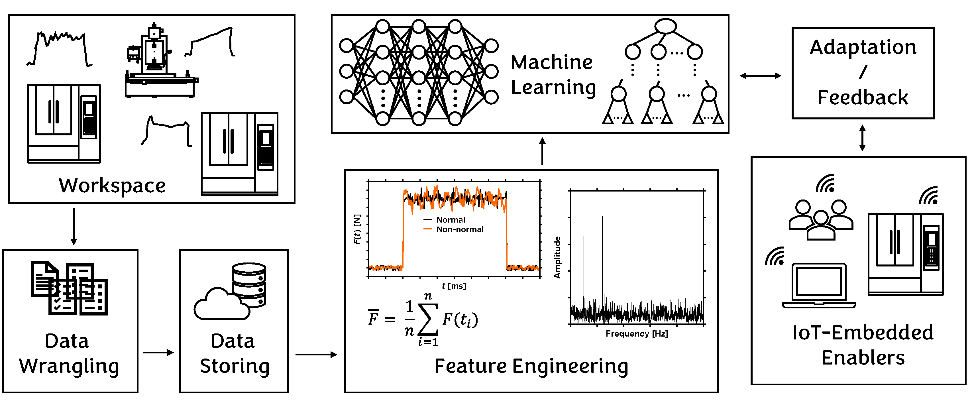
Figure 2.
Context of this study.
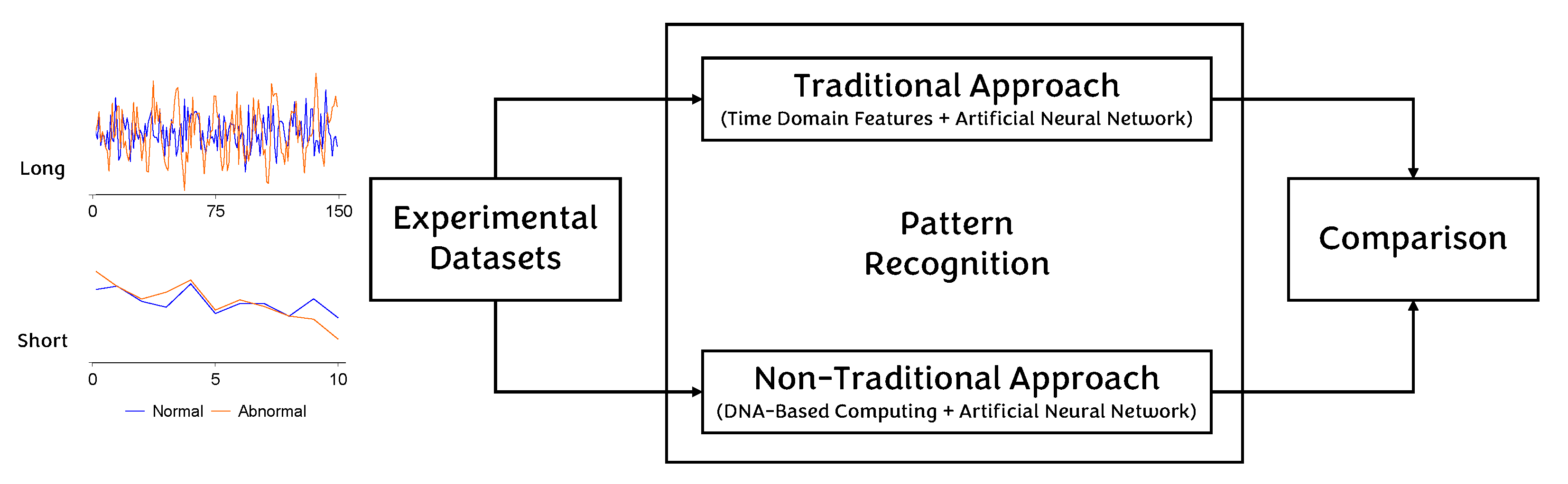
Figure 3.
Instances of prepared datasets for long window (a, c, and e) and short window (b, d, and f).
Figure 3.
Instances of prepared datasets for long window (a, c, and e) and short window (b, d, and f).
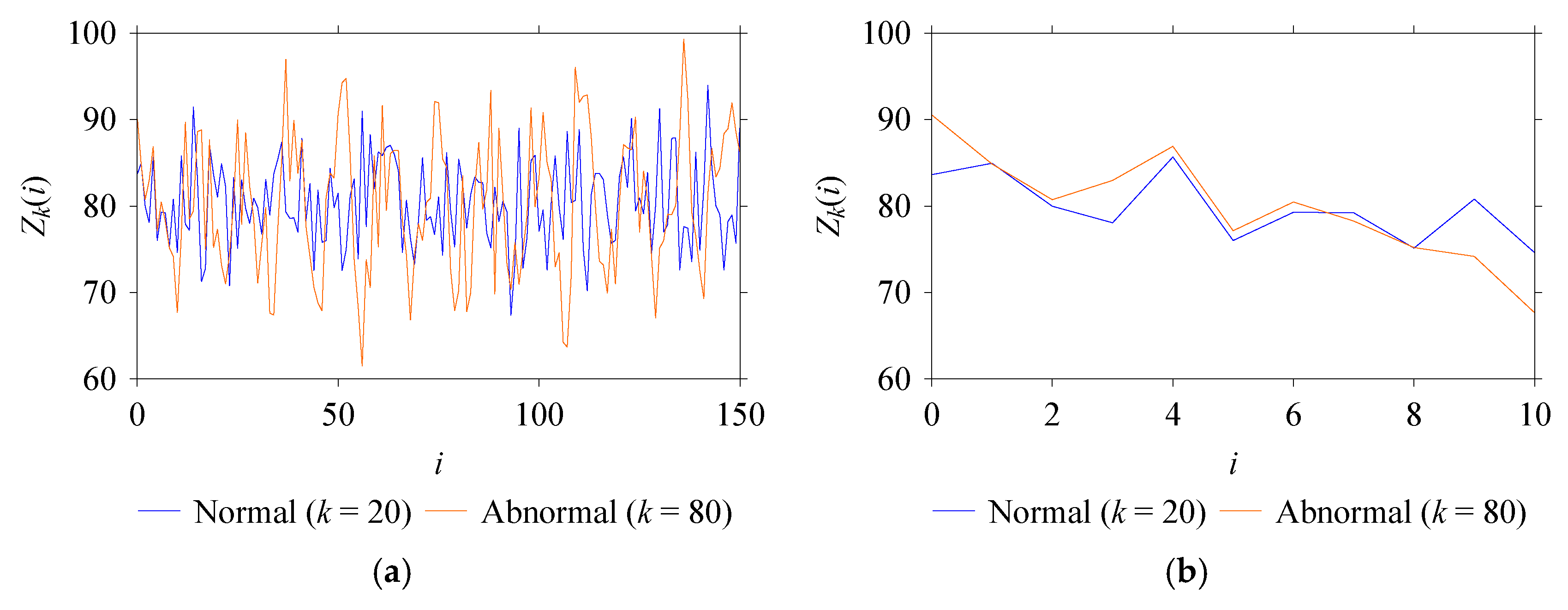
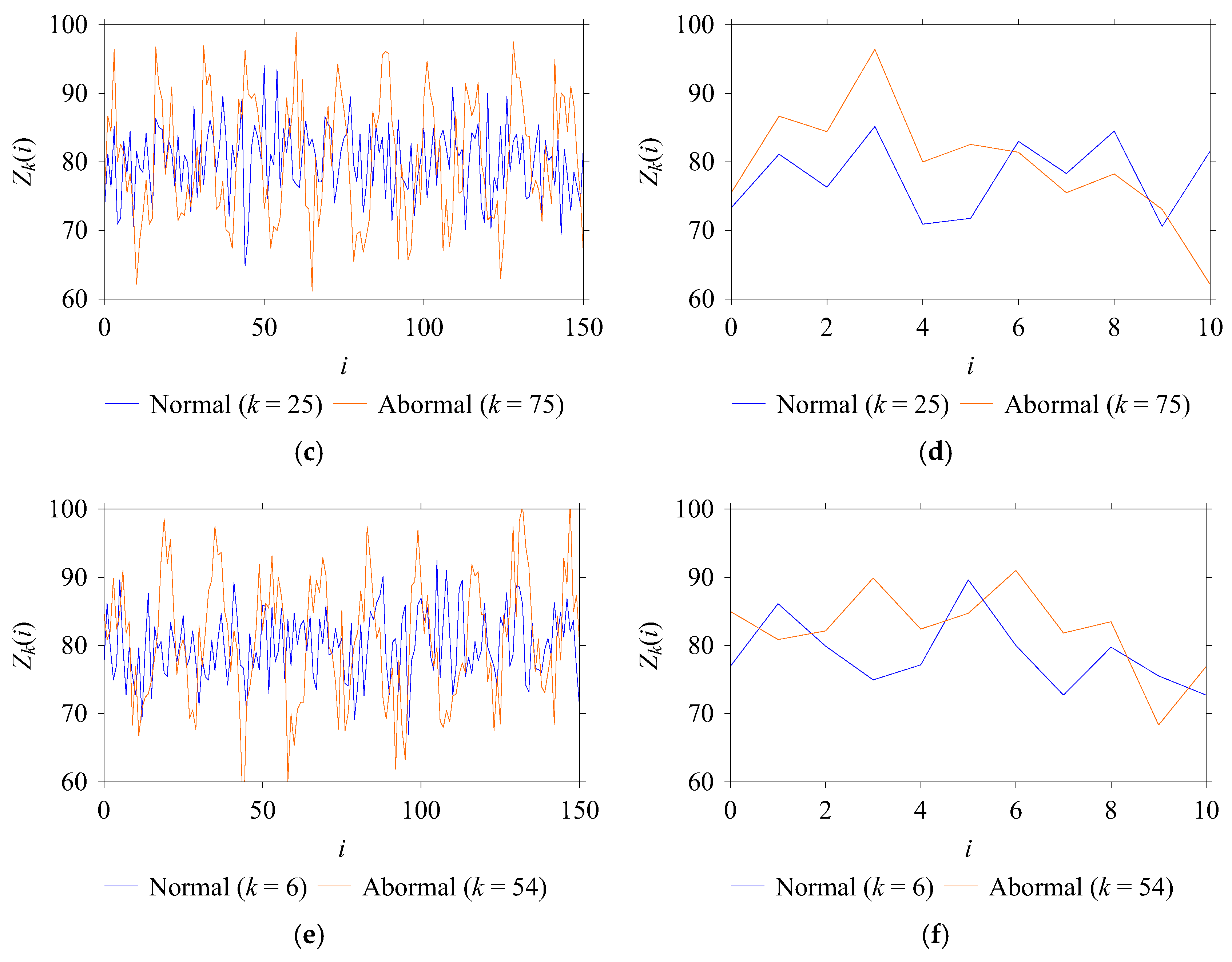
Figure 4.
Outlining a traditional feature engineering-based ANN approach for pattern recognition.
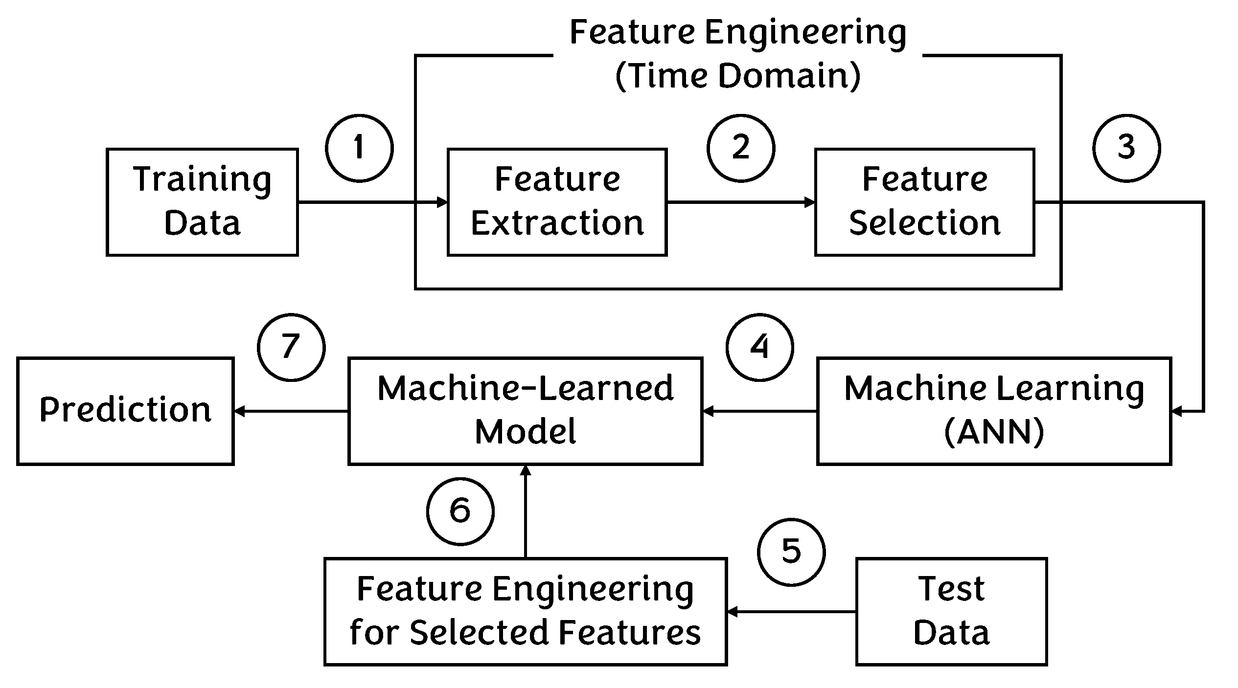
Figure 5.
Outlining (a) DNA-Based Computing (DBC) and (b) Proposed DBC-ANN approach for pattern recognition.
Figure 5.
Outlining (a) DNA-Based Computing (DBC) and (b) Proposed DBC-ANN approach for pattern recognition.
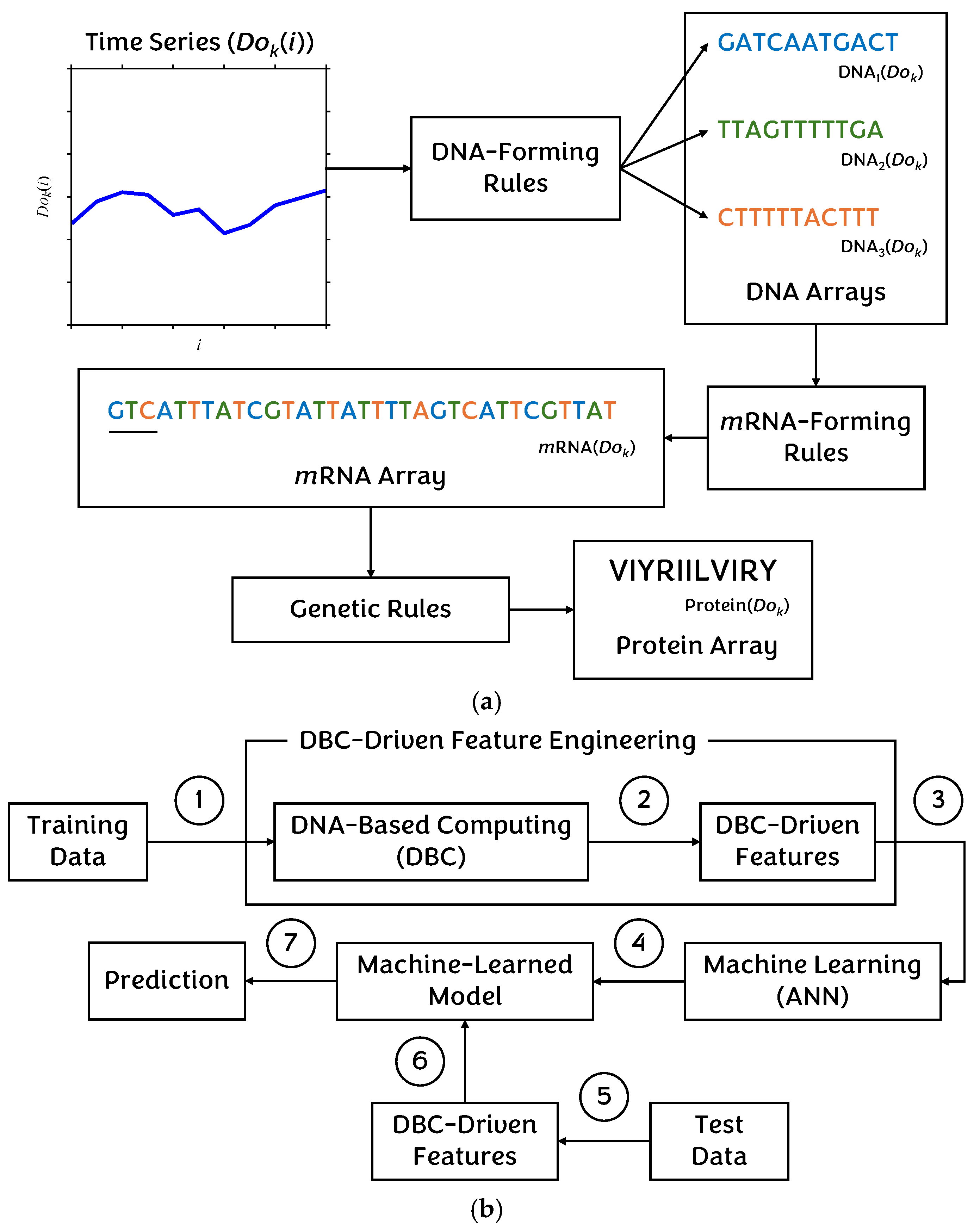
Figure 6.
Feature space extracted from long window-driven training datasets.
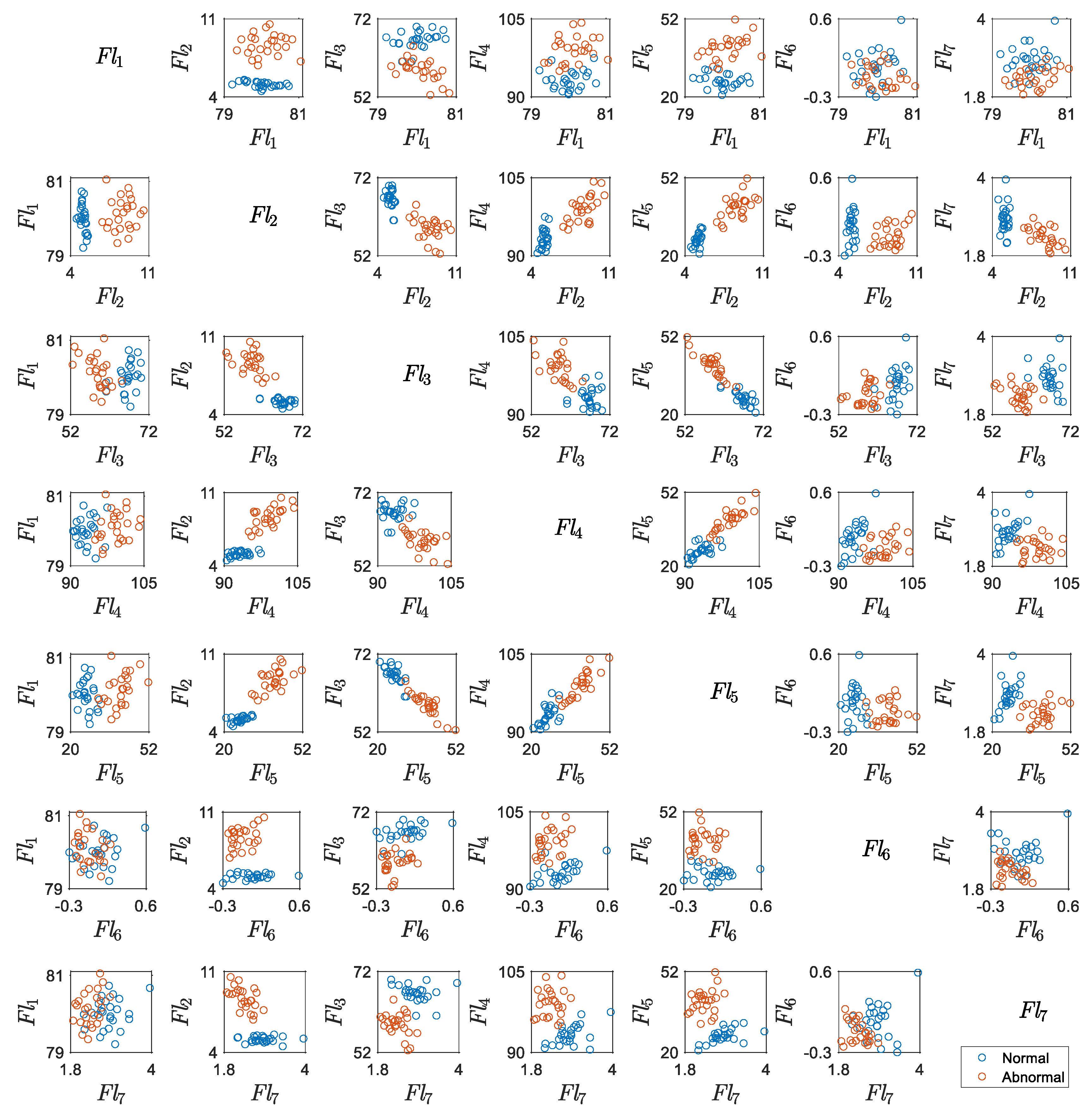
Figure 7.
Feature space extracted from short window-driven training datasets.
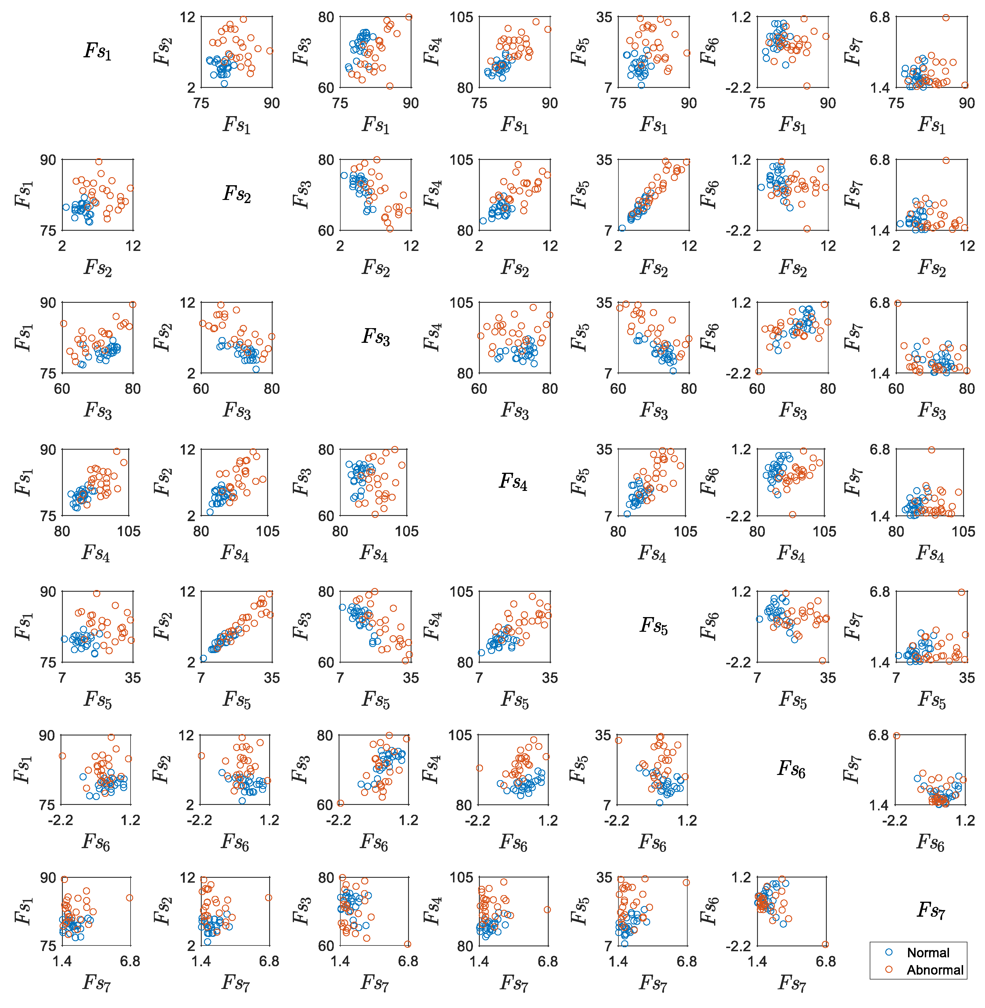
Figure 8.
Feature importance score for: (a) long window, (b) short window.
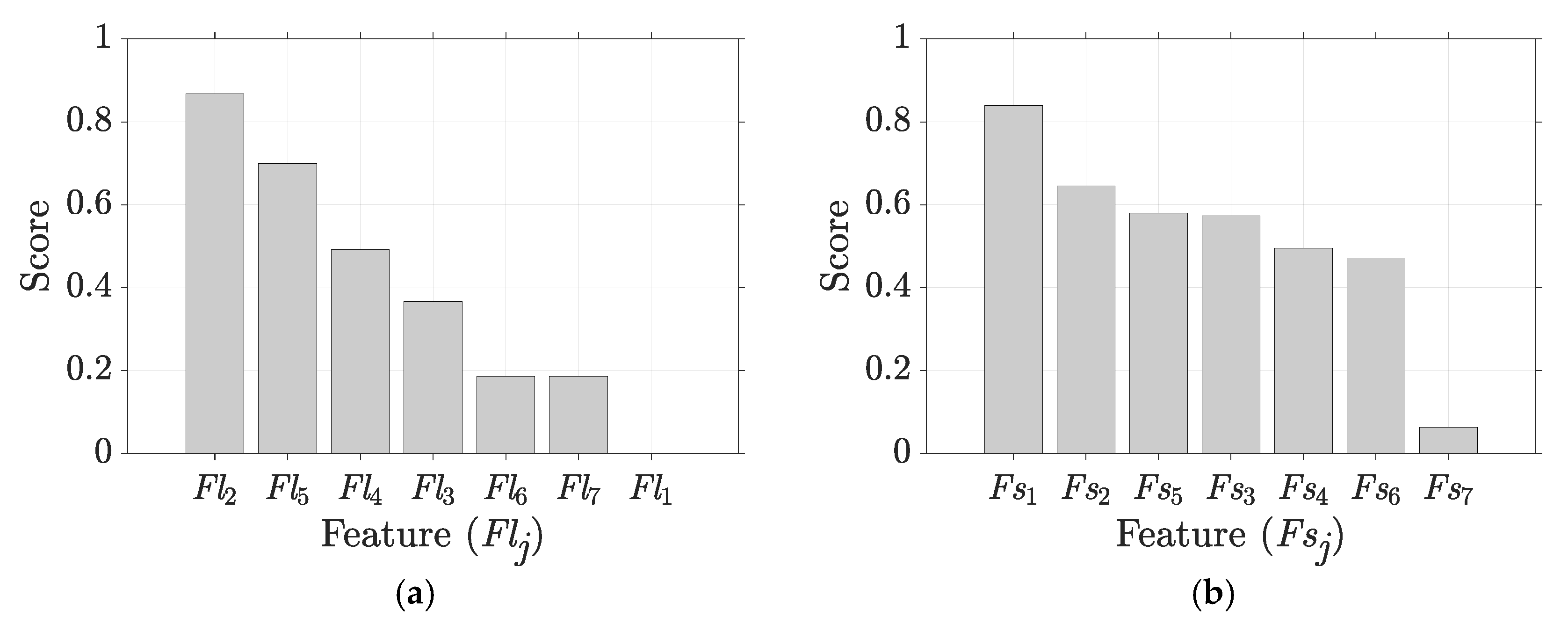
Figure 9.
Performance of feature-based ANN model subjected to long window in: (a) training phase, (b) testing phase.
Figure 9.
Performance of feature-based ANN model subjected to long window in: (a) training phase, (b) testing phase.
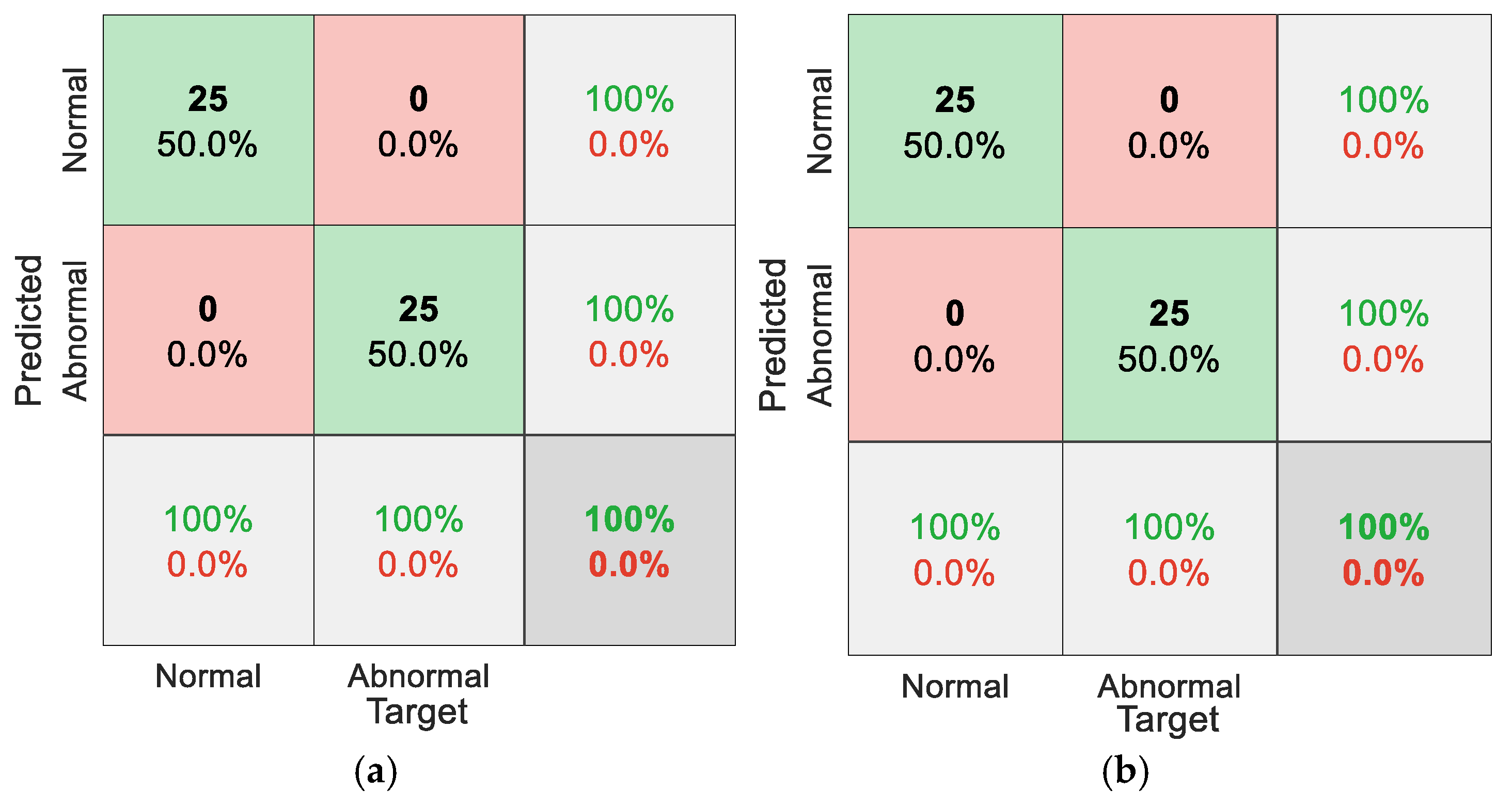
Figure 10.
Performance of feature-based ANN model subjected to short window in: (a) training phase, (b) testing phase.
Figure 10.
Performance of feature-based ANN model subjected to short window in: (a) training phase, (b) testing phase.
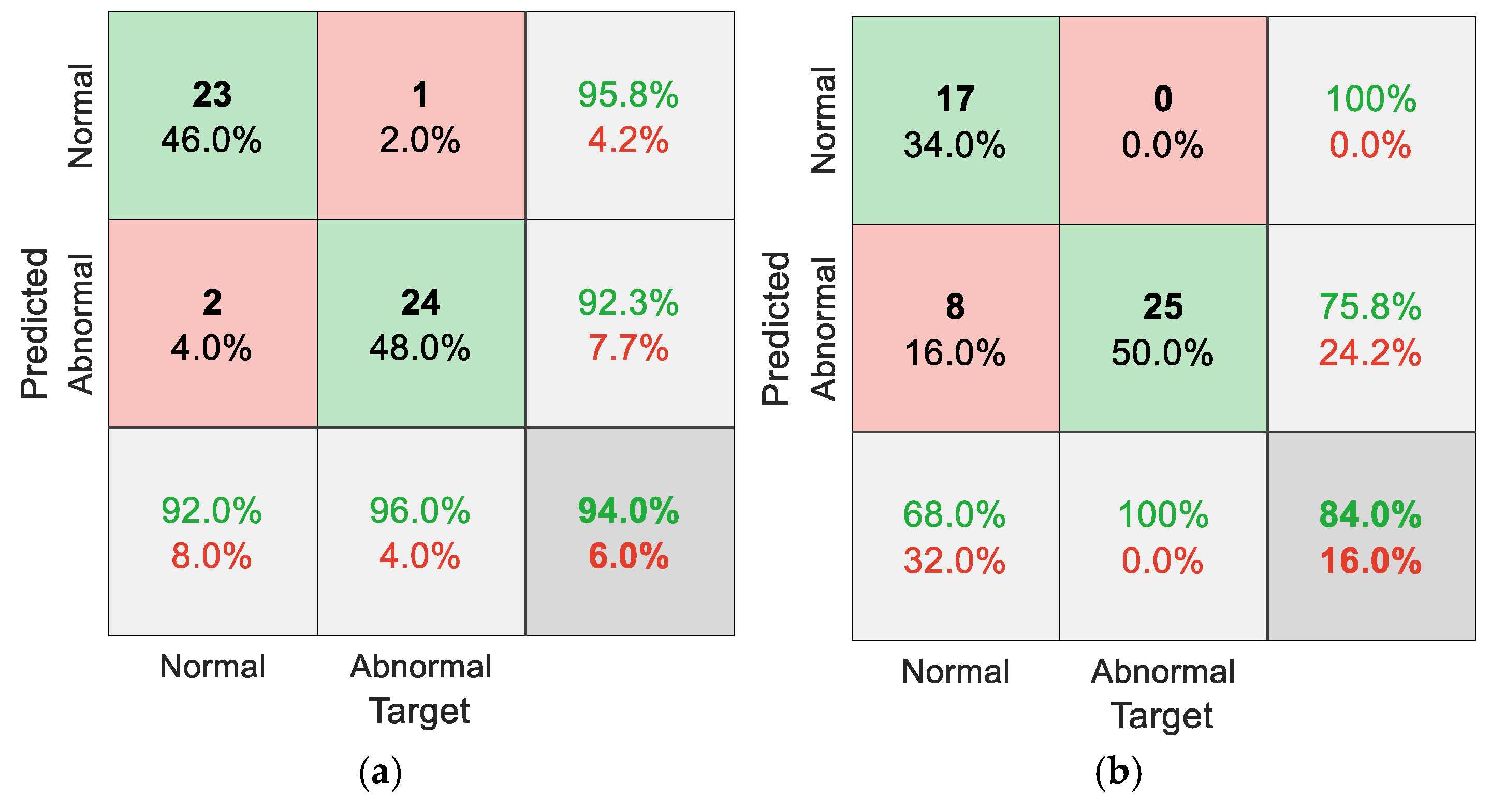
Figure 11.
Outcomes of type-2 DBC for long window-driven training datasets: (a) interplay of protein arrays and their constituents in the protein-verse, (b) instances of interplay.
Figure 11.
Outcomes of type-2 DBC for long window-driven training datasets: (a) interplay of protein arrays and their constituents in the protein-verse, (b) instances of interplay.
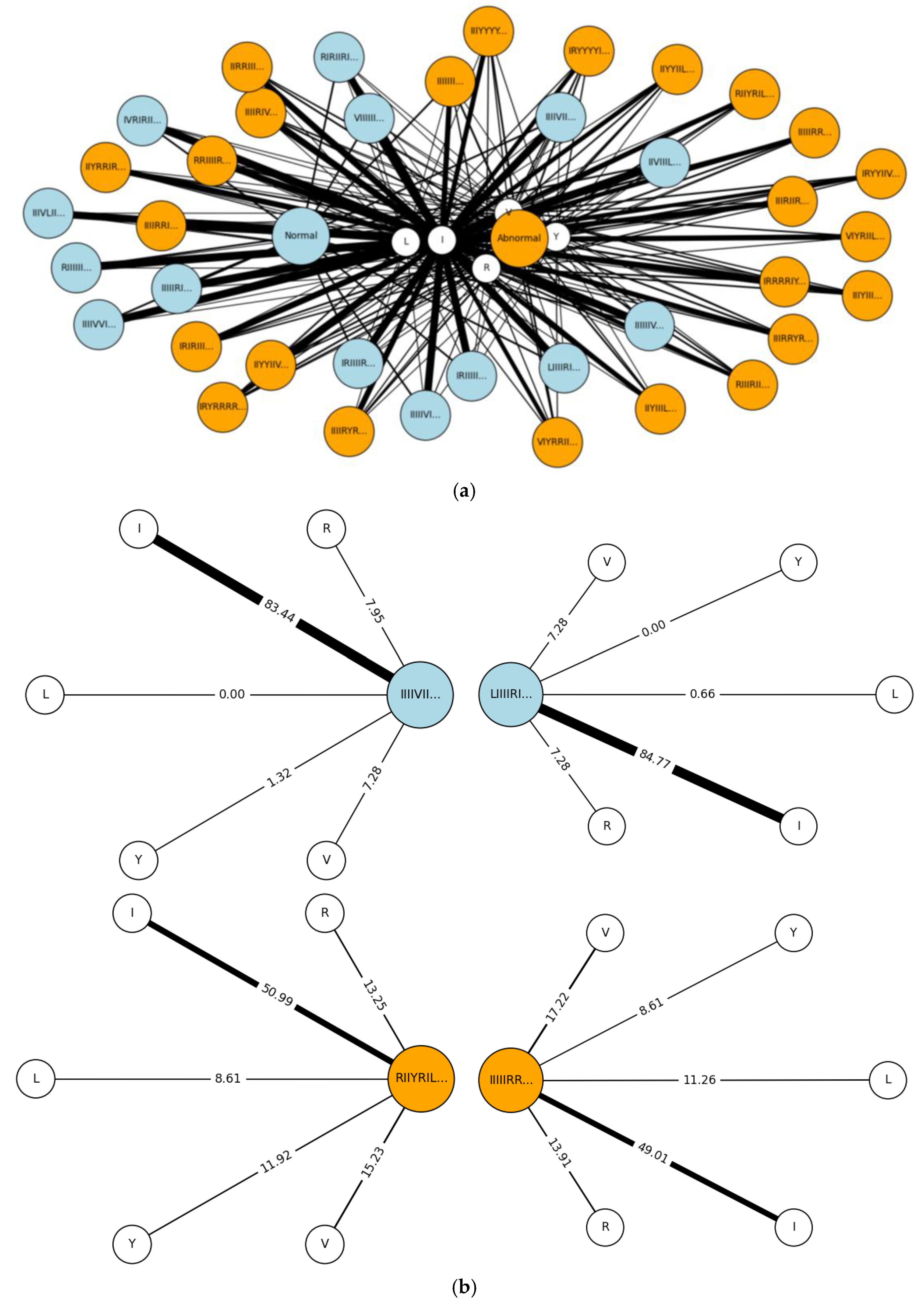
Figure 12.
Outcomes of type-2 DBC for short window-driven training datasets: (a) interplay of protein arrays and their constituents in the protein-verse, (b) instances of interplay.
Figure 12.
Outcomes of type-2 DBC for short window-driven training datasets: (a) interplay of protein arrays and their constituents in the protein-verse, (b) instances of interplay.
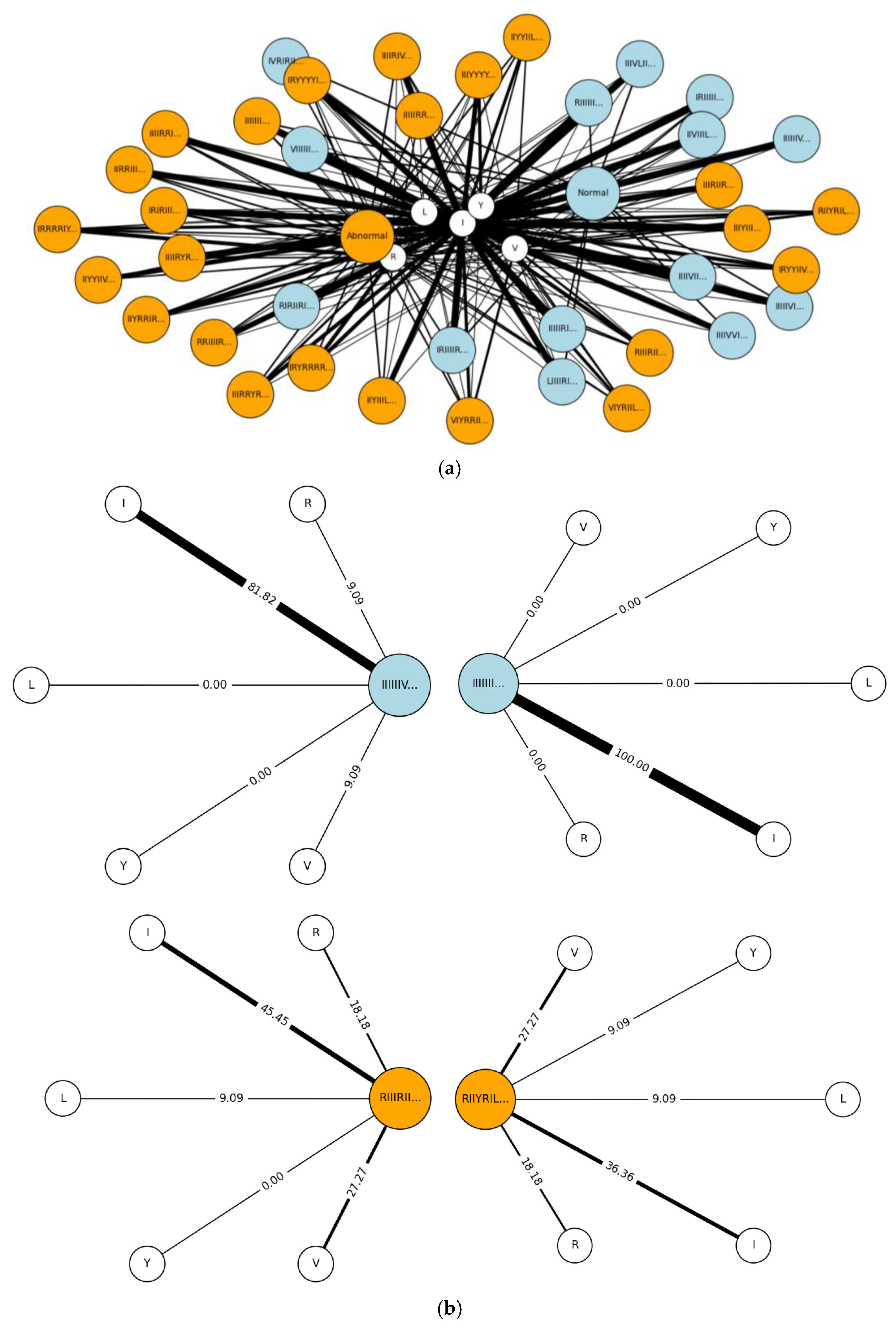
Figure 13.
Hamming distances between normal and abnormal arrays for: (a) long window-driven training datasets, (b) short window-driven training datasets.
Figure 13.
Hamming distances between normal and abnormal arrays for: (a) long window-driven training datasets, (b) short window-driven training datasets.
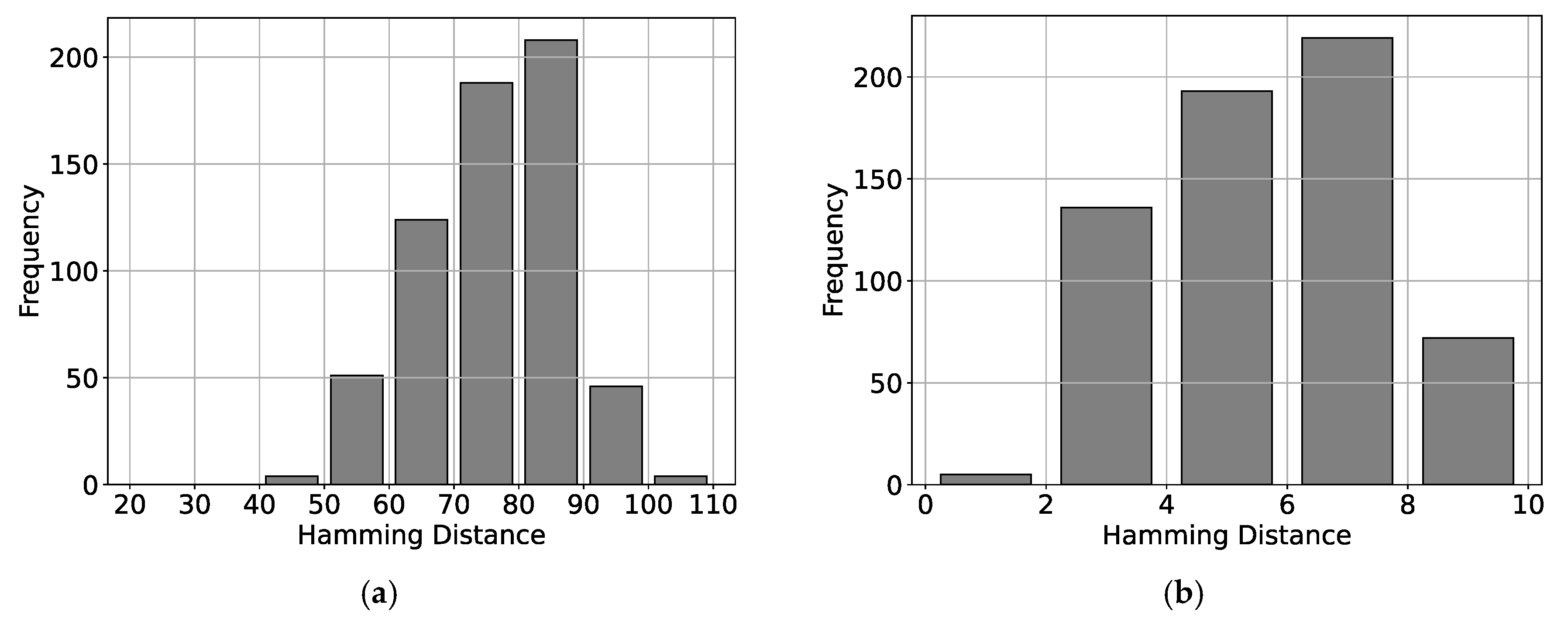
Figure 14.
Performance of DBC-based ANN model subjected to long window in: (a) training phase, (b) testing phase.
Figure 14.
Performance of DBC-based ANN model subjected to long window in: (a) training phase, (b) testing phase.
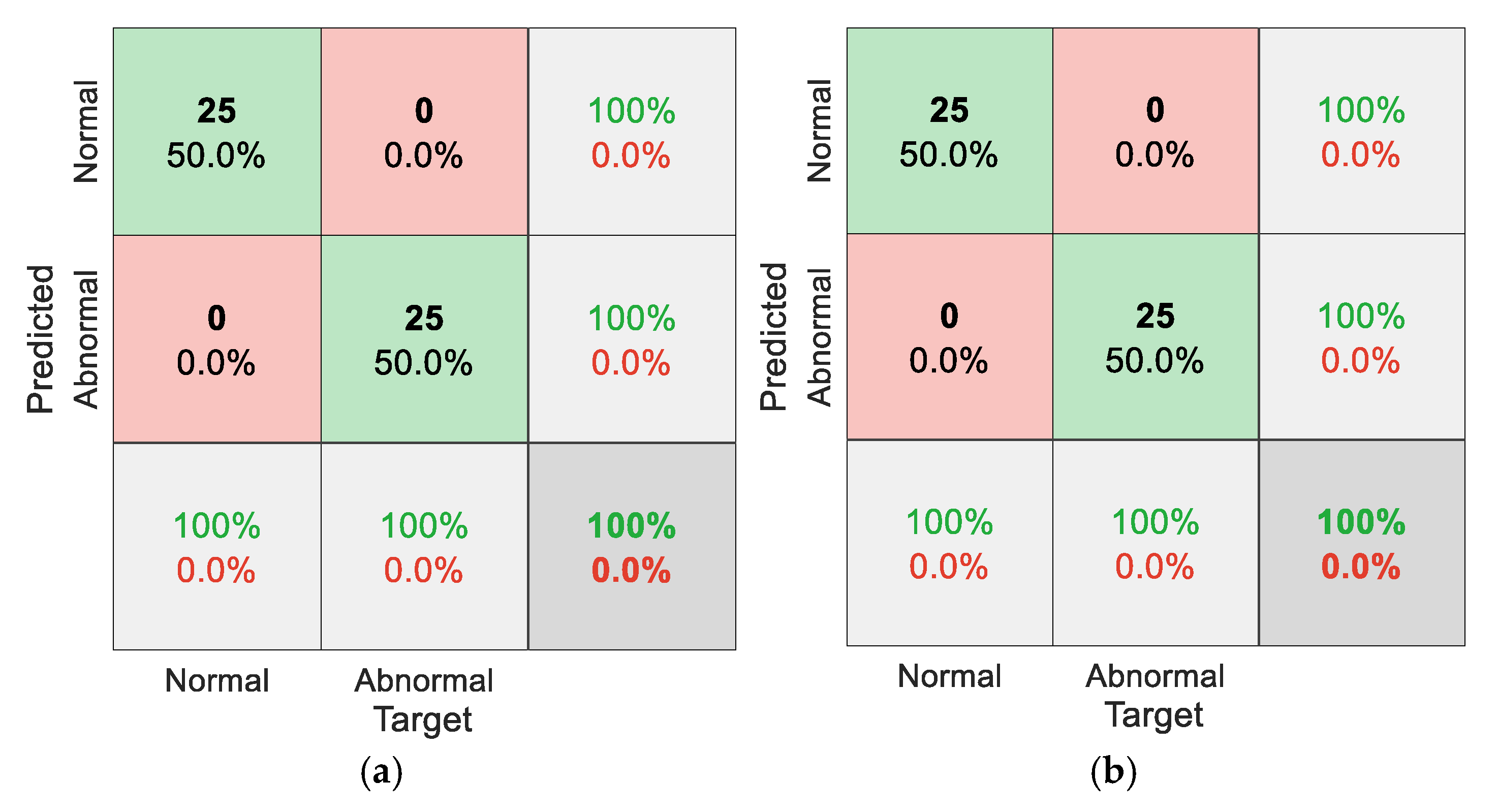
Figure 15.
Performance of DBC-based ANN model subjected to short window in: (a) training phase, (b) testing phase.
Figure 15.
Performance of DBC-based ANN model subjected to short window in: (a) training phase, (b) testing phase.

Figure 16.
20-fold Monte Carlo Cross-Validation for feature-based ANN when window is short: (a) training and testing accuracy per fold, (b) accuracy difference per fold.
Figure 16.
20-fold Monte Carlo Cross-Validation for feature-based ANN when window is short: (a) training and testing accuracy per fold, (b) accuracy difference per fold.
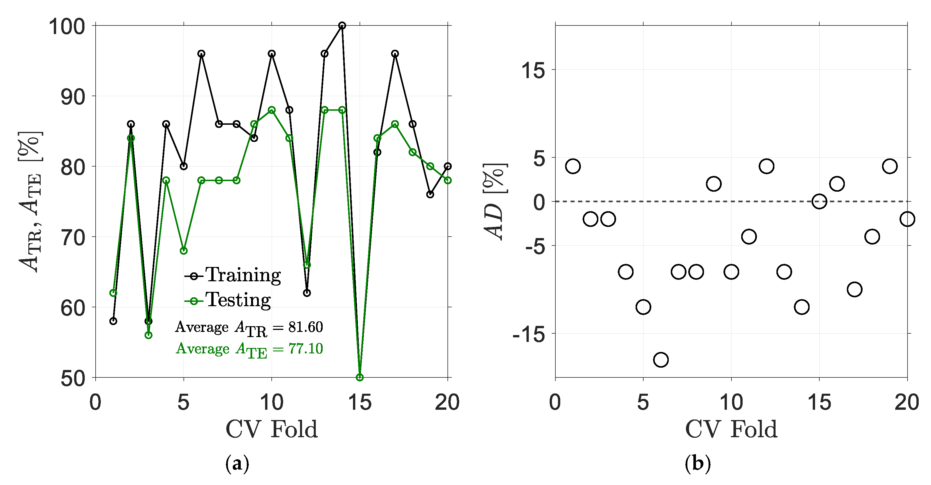
Figure 17.
20-fold Monte Carlo Cross Validation for DBC-based ANN when window is short: (a) training and testing accuracy per fold, (b) accuracy difference per fold.
Figure 17.
20-fold Monte Carlo Cross Validation for DBC-based ANN when window is short: (a) training and testing accuracy per fold, (b) accuracy difference per fold.
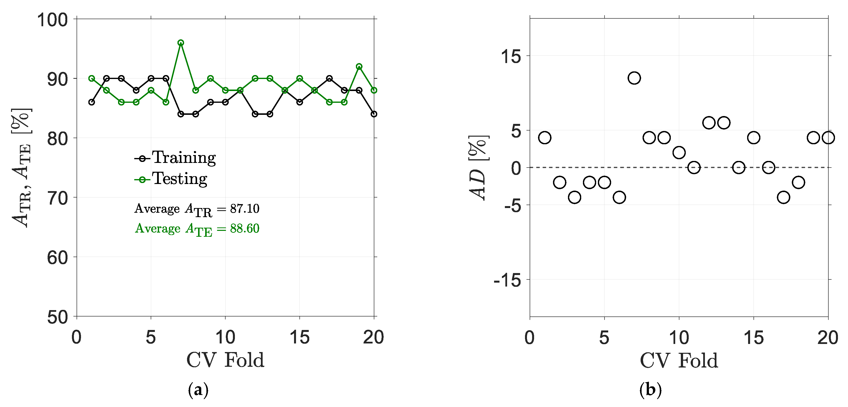

Table 1.
Outlining data preparation.
| Steps | Description | |
|---|---|---|
| Creation | 100 datasets are created, of which 50 are “Normal” and 50 are “Abnormal,” following the definitions in [30]. | |
| Splitting | Using stratified sampling, the created datasets are divided into a training set and a test set, each containing 50 datasets. | |
| Windowing | Long | The training and test sets are processed with a long window size of 150, resulting in long-windowed datasets. |
| Short | The training and test sets are processed with a short window size of 10, resulting in short-windowed datasets. | |
Disclaimer/Publisher’s Note: The statements, opinions and data contained in all publications are solely those of the individual author(s) and contributor(s) and not of MDPI and/or the editor(s). MDPI and/or the editor(s) disclaim responsibility for any injury to people or property resulting from any ideas, methods, instructions or products referred to in the content. |
© 2025 by the authors. Licensee MDPI, Basel, Switzerland. This article is an open access article distributed under the terms and conditions of the Creative Commons Attribution (CC BY) license (http://creativecommons.org/licenses/by/4.0/).
Copyright: This open access article is published under a Creative Commons CC BY 4.0 license, which permit the free download, distribution, and reuse, provided that the author and preprint are cited in any reuse.


