
Submitted:
25 June 2025
Posted:
30 June 2025
You are already at the latest version
Abstract
Hybrid modeling techniques are increasingly important for improving predictive accuracy and control in biomanufacturing, particularly under data-limited conditions. This study focuses on the development and experimental validation of a hybrid deep learning model predictive control (MPC) framework for fed-batch P. pastoris fermentations producing recombinant proteins. Bayesian optimization and grid search were employed to identify optimal network architectures, revealing that models combining LSTM layers with fully connected layers provided the best balance between prediction accuracy and computational efficiency. The top-performing architecture was adapted to a new dataset involving bacteriophage Qβ coat protein production using transfer learning, yielding strong predictive performance with low validation and test losses. Experimental implementation of the novel hybrid MPC system demonstrated robust real-time control of substrate feeding to maintain target specific growth rates. While moderate discrepancies were observed in biomass and product predictions—particularly during the methanol adaptation phase and late-stage cytotoxic conditions—the controller effectively regulated process dynamics. These findings suggest that hybrid neural networks, when integrated with MPC and refined through automated architecture selection, offer a practical and generalizable solution for real-time control in microbial bioprocesses. This work provides a validated framework for deploying hybrid digital twins in fermentation and highlights the need to account for physiological effects in future models.
Keywords:
Pichia Pastoris
; hybrid process model
; deep learning
; Bayesian optimization
; hybrid model architecture screening
; transfer learning
; model predictive control
; hybrid MPC
1. Introduction
The inherent complexity of biological systems—characterized by interconnected subsystems and nonlinear dynamics— presents enduring challenges for effective bioprocess monitoring and control. Mathematical modeling offers a powerful means to capture and manage this complexity [1]. Over the past few decades, such models have become indispensable in understanding and optimizing bioprocesses, benefiting from advances in computational capabilities and analytical tools. This progress has led to the adoption of advanced modeling approaches, such as genome-scale metabolic models and computational fluid dynamics simulations [2,3]. With the advent of Industry 4.0, modeling has taken on an even more prominent role in the digital transformation of biomanufacturing [4]. However, the limitations of mechanistic models—particularly their reliance on complete system knowledge—have prompted interest in alternative strategies. As a result, machine learning techniques are gaining traction, offering flexible, data-driven alternatives that can extract insights without relying on fully defined system knowledge—supporting next-generation bioprocess digitalization [5,6,7,8].
To bridge this gap, hybrid neural network (HNN) models have emerged as a compelling solution, integrating domain knowledge with data-driven flexibility [9,10,11,12,13,14]. These models combine the structure of mechanistic frameworks (e.g., mass or energy balances) with the flexibility of data-driven components such as ANNs, effectively leveraging both physical laws and empirical data [15,16]. A typical use case involves modeling unknown or complex kinetics using neural networks within a differential equation-based framework. Compared to purely nonparametric models, hybrid approaches often yield more accurate, generalizable, and interpretable results—leading to more robust bioprocess operation and control [17]. The recent surge in deep learning methodologies has further enhanced hybrid modeling by enabling neural networks to approximate intricate biological functions, as deep neural networks (DNNs) with multiple hidden layers have demonstrated superior capacity for learning hierarchical and compositional functions with fewer parameters and reduced sample complexity compared to shallow architectures [9,10,18]. As such, hybrid deep learning models are emerging as a powerful tool in the development of digital twins and advanced bioprocess monitoring systems.
In parallel, deep learning developments have expanded modeling capabilities across bioprocess applications. DNNs, through their multilayered architectures, enable the extraction of hierarchical and compositional features, allowing for the accurate approximation of highly nonlinear biological dynamics [18,19]. These models have demonstrated strong performance across a range of bioprocessing tasks, including soft sensing, anomaly detection, forecasting, and system identification, particularly when applied to high-resolution data streams generated by modern process analytical technologies (PAT). Long Short-Term Memory (LSTM) networks, designed to retain temporal context over extended time horizons, have proven especially valuable for modeling dynamic bioreactor cultivations. When coupled with mechanistic models, LSTMs form powerful hybrid frameworks capable of accurately capturing both short-term variability and long-term process trends [11]. Critical to the effective training of such deep architectures are modern optimization and activation strategies: the rectified linear unit (ReLU) activation function addresses vanishing gradient problems, while the Adaptive Moment Estimation (Adam) optimizer accelerates convergence and enhances generalization through adaptive learning rate adjustments [10,20]. Collectively, these innovations position deep hybrid modeling as a central enabler of next-generation digital twins for real-time monitoring, control, and optimization in biomanufacturing.
However, training deep models requires extensive, high-frequency datasets that are often unavailable in bioprocessing due to high costs, long cultivation times, and sensor limitations [21]. In early-stage bioprocess development or pilot-scale operations, datasets typically contain only a small number of replicates per condition, resulting in limited coverage of the process space and insufficient diversity to support generalizable deep models [22]. Bioprocess data is typically noisy, heterogeneous, and expensive to generate, posing a major bottleneck for training deep architectures. Such data limitations have accelerated the adoption of hybrid modeling frameworks, which leverage both prior process knowledge and empirical data. The promising approach of integrating historical process data through transfer learning frameworks can significantly improve prediction accuracy and reduce the need for extensive new experimental data [23,24].
Transfer learning (TL) in deep neural networks involves repurposing a model trained on a source task to enhance learning on a related target task, especially when labeled data are scarce. By leveraging pre-trained models—often developed on large, generic datasets—TL facilitates improved convergence speed, generalization, and computational efficiency compared to training from scratch [25,26]. In bioprocess engineering, TL enables the adaptation of models trained on well-characterized systems to predict dynamics in novel or data-limited processes. For instance, TL has been successfully applied to model microalgal bioprocess dynamics using limited time-series data, achieving high accuracy in forecasting process behavior [27] and for the quantification and identification of cellular phenotypes from high-content microscopy images [28].
Despite its advantages, TL poses challenges such as negative transfer, which occurs when source and target domains are insufficiently aligned, and catastrophic forgetting during fine-tuning [29]. Effective transfer requires careful selection of source models, layer-freezing strategies, and learning rate tuning to preserve useful features while adapting to the new task. In bioprocess applications, these considerations are critical due to the heterogeneity of biological systems and the frequent lack of large annotated datasets. Nevertheless, TL remains a promising strategy—especially when combined with hybrid modeling approaches that integrate mechanistic insights with data-driven learning [30].
Deep neural network architecture screening typically involves systematic strategies to identify optimal model configurations and hyperparameters. Common methods include grid search, which exhaustively evaluates combinations within a predefined parameter grid [31]. While easy to implement and parallelize, grid search becomes computationally expensive as the number of hyperparameters increases. Random search improves efficiency by sampling configurations at random, often outperforming grid search in high-dimensional spaces where only a few parameters significantly affect performance [31]. A more advanced and efficient approach is Bayesian optimization, which builds a probabilistic surrogate model (e.g., Gaussian Process) to predict performance and selects promising configurations using acquisition functions like Expected Improvement [32]. This strategy significantly reduces the number of required evaluations and is especially valuable when model training is computationally costly. Several studies confirm that Bayesian optimization typically outperforms traditional approaches in terms of sample efficiency and final model performance [31,32].
As the dominant production mode, fed-batch fermentation remains widely used due to its robustness and high product yields, with most biotherapeutics in clinical and commercial use produced using this mode [33,34]. However, maintaining optimal substrate feeding remains a major challenge, requiring precise control to ensure consistent performance. Model Predictive Control (MPC) has emerged as a powerful strategy to address this, leveraging predictive models to optimize feeding decisions in real time [35,36]. Yet, the nonlinear and dynamic nature of high cell density fermentations often limits the accuracy of purely mechanistic models, as parameter estimation and unforeseen biological interactions degrade model reliability [33,37]. Hybrid modeling strategies help mitigate these challenges by improving parameter adaptability, accounting for process nonlinearities, and enhancing real-time prediction accuracy [38]. Integrating hybrid bioreactor process models with MPC enhances the optimization and control of bioprocesses, particularly in complex systems like high cell density fermentations, resulting in improved modelling accuracy, increased adaptability to changing process conditions and real-time feed-back for increased process stability [39,40,41].
The selection of an appropriate expression system is a critical factor in recombinant protein production, as it directly influences yield, functionality, and downstream processing. Among the various platforms available, the methylotrophic yeast Pichia pastoris has emerged as a preferred host over the past two to three decades for both research and industrial applications. It offers several advantages, including ease of genetic manipulation, high transformation efficiency, and the ability to achieve high protein titers both intracellularly and extracellularly [42,43]. Furthermore, P. pastoris supports essential eukaryotic post-translational modifications such as glycosylation, disulfide bond formation, and proteolytic processing, making it well-suited for producing complex proteins. Its minimal native protein secretion simplifies purification, and its capacity for rapid growth in defined media, along with robust genetic tools and stable expression over extended cultivation periods, strengthens its suitability for scalable production. These characteristics along with growing interest in digital bioprocessing, make P. pastoris a strong candidate for hybrid model development and advanced biomanufacturing strategies [44,45].
The Qβ coat protein virus-like particles (VLPs) are self-assembling, non-infectious nanostructures derived from the bacteriophage Qβ. These VLPs have garnered significant attention in biomedicine due to their uniform size, stability, and ability to present antigens in a repetitive, high-density manner, which is highly effective in eliciting strong immune responses. Notably, Qβ VLPs have been successfully utilized in vaccine development [46,47]. Furthermore, their versatility allows for the encapsulation of various cargos, making them valuable in drug delivery and nanotechnological applications. Qβ VLPs can be efficiently produced in P. pastoris, a widely used yeast expression system, which offers high-yield, cost-effective recombinant protein production with proper protein folding and scalability for biopharmaceutical applications [48].
Recent work has explored hybrid modeling in recombinant P. pastoris cultivations, demonstrating performance gains in process control, generalization, and scalability. Ferreira et al. used a serial HNN, consisting of a three-layer feedforward neural network (FFNN) combined with material balance equations, for dynamic modeling of P. pastoris GS115 expressing scFv in a 50 L pilot bioreactor. This hybrid model was then applied for iterative batch-to-batch control, resulting in a 4-fold increase in titer after four optimization cycles [12]. Pinto et al. revisited the general bioreactor hybrid model and introduced deep learning techniques. Multi-layer networks with varying depths were combined with First Principles equations to form deep hybrid models. Techniques like ADAM, stochastic regularization, and depth-dependent weight initialization were evaluated in this context. The methods were applied to a synthetic E. coli dataset and a 50 L Mut+ P. pastoris process expressing a single-chain antibody fragment. Results showed significant improvements in generalization, with an 18.4% increase in prediction accuracy and a 43.4% reduction in CPU time compared to shallow models [10]. In another study, Pinto et al. developed a hybrid deep modeling method with state-space reduction, applied to a P. pastoris GS115 Mut+ strain expressing scFv. Deep FFNNs of varying depths were combined with bioreactor material balance equations and trained using ADAM, semidirect sensitivity equations, and stochastic regularization. A state-space reduction method, based on principal component analysis (PCA) of the cumulative reacted amount, reduced model complexity by 60% and improved predictive accuracy by 18.5%. Validation with data from nine fed-batch P. pastoris 50 L cultivations highlighted optimization opportunities, with potential increases in scFv titer of 30% and 80% by optimizing methanol feed and inorganic elements, respectively [9].
This study presents a hybrid deep learning model tailored to recombinant P. pastoris fermentations, trained using a transfer-learning approach of historical and newly acquired batch data, incorporating both at-line and in-line biomass measurements. The model architecture integrates mechanistic knowledge with data-driven components to effectively capture the complex dynamics of the fermentation process. The resulting model is integrated into a novel Model Predictive Control framework, enabling adaptive feeding strategies and dynamic trajectory tracking. We validate the approach through an experimental fermentation run, showcasing improved control precision and enhanced process stability.
2. Materials and Methods
Experimental conditions
Cultivations were performed using a recombinant Pichia pastoris X-33 wild-type strain producing Qβ coat protein VLPs. The construction of the expression vector and the selection of clones for this specific producer are described in detail elsewhere [48].
The batch and feed media formulations were prepared following the “Pichia Fermentation Process Guidelines” provided by Invitrogen Corporation [49]: 1.9 L of Basal Salts Medium (26.7 mL·L−1 H3PO4 85%, 0.93 g·L−1 CaSO4, 18.2 g·L−1 K2SO4, 14.9 g·L−1 MgSO4·7H2O, 4.13 g·L−1 KOH, 40.0 g·L−1 glycerol and 4.35 mL·L-1 PTM1 trace element solution (0.02 g·L−1 H3BO4, 5 mL·L−1 H2SO4 98%, 6.0 g·L−1 CuSO4·5H2O, 0.08 g·L−1 NaI, 3.0 g·L−1 MnSO4·H2O, 0.2 g·L−1 Na2MoO4·2H2O, 0.5 g·L−1 Ca2SO4·2H2O, 20.0 g·L−1 ZnCl2, 65.0 g·L−1 FeSO4·7H2O, 0.2 g·L-1 biotin)), was inoculated with 100 mL of inoculum grown in BMGY medium (10.0 g·L-1 yeast extract, 20.0 g·L-1 peptone, 100 mM potassium phosphate buffer, pH 6.0, 13.4 g·L-1 yeast nitrogen base, 10.0 g·L-1 glycerol, 0.0004 g·L-1 biotin) at 30°C for 18-22 h in a shake flask at 250 RPM. Two feeding solutions were used: a glycerol feed consisting of 50% v/v glycerol and 12 mL·L⁻¹ PTM1, and a methanol fed-batch solution composed of 100% methanol with 12 mL·L⁻¹ PTM1.
The bioreactor vessel was filled with distilled water and sterilized at 121 °C for 30 minutes. BSM, BMGY, and the glycerol fed-batch solutions were autoclaved separately under the same conditions. The PTM1 trace element solution was sterilized by filtration using a 0.2 µm membrane filter.
Fermentations were carried out in a 5 L bench-top bioreactor (Bioreactors.net, EDF-5.4/BIO-4, Latvia) with a working volume of 2–4 L, as illustrated in Figure 2. The pH was continuously monitored using a calibrated pH probe (Hamilton, EasyFerm Bio, Switzerland) and adjusted to 5.0 ± 0.1 with a 28% NH₄OH solution prior to inoculation, then maintained at this value throughout the process. Temperature was regulated at 30.0 ± 0.1 °C using a temperature sensor and jacketed vessel control. A thermostatic circulator (LKB Bromma, Multitemp II, Sweden) maintained the cooling water at a preset temperature of 6 °C during experiments.
Dissolved oxygen (DO) levels were measured using a DO sensor (Hamilton, Oxyferm Bio, Switzerland) and maintained above 30 ± 5% via a dual cascade strategy: adjusting the stirrer speed between 200–1000 RPM (Cascade 1), and supplementing the inlet air with pure O₂ when necessary (Cascade 2). A constant airflow or air/oxygen mixture at 3.0 slpm was sustained throughout the fermentation. A condenser was employed to capture moisture from exhaust gases, and Antifoam 204 (Sigma) was added as needed to suppress excessive foam formation. Substrate feeding was controlled with a high-precision peristaltic pump (Longer-Pump, BT100–2J, China).
The cultivations began with a glycerol batch phase. After 18–20 hours, once the batch glycerol was depleted, a glycerol fed-batch phase was initiated by feeding the reactor with a glycerol solution at a rate of 0.61 mL·min⁻¹ for 4 hours, or until an optical density (OD) of 100–120 was reached. Following a short feeding pause of 5–20 minutes—allowing the cells to consume any residual glycerol—the substrate was switched to methanol. Methanol feeding proceeded in three phases: initially at 0.12 mL·min⁻¹ for 5 hours, then at 0.24 mL·min⁻¹ for 2 hours, and finally at 0.36 mL·min⁻¹, which continued either until the end of the experiment or for 2–3 hours until the hybrid MPC control was activated.
In experiments where real-time biomass concentration was monitored using an in-situ turbidity probe (Optek-Danulat, ASD19-EB-01, Germany), the turbidity signal was correlated with biomass concentration using an exponential calibration equation reported previously [50]. To enhance signal reliability, an algorithm was implemented to correct for abrupt spikes caused by sudden process disturbances. The details of this algorithm are provided in a separate publication [51].
Although the cultivation conditions were generally similar across all historical experiments, some minor differences were present. For detailed information on these variations, as well as the construction of the expression vectors and clone selection, we refer the reader to the original publications [44,52].
Downstream processing of Qβ VLPs
4.0 g of wet cells were resuspended in 20 mL of lysis buffer (20 mM Tris 8.0, 100 mM NaCl) and disrupted by French press (4x 10,000 psi). The suspension was then centrifuged for 30 min at 18,500 g (4°C). Ammonium sulfate was added to the supernatant to 40% saturation and proteins precipitated at 4°C for 60 minutes. The suspension was then centrifuged for 20 min at 18,500 g (4°C) and the supernatant discarded. Precipitate was dissolved in 20 mM Tris 8.0 buffer and loaded onto Sepharose 4 Fast Flow size-exclusion column (12 mL volume) in lysis buffer at 0.3 mL/min. Peak fractions were pooled and loaded onto anion-exchange Fractogel DEAE (M) column (5 mL volume) in lysis buffer and eluted with a linear gradient of 20 mM Tris-HCl, 1 M NaCl pH 8.0 at 2 mL/min.
Analytical measurements
Cell growth was observed by off-line measurements of dry cell weight (DCW), determined gravimetrically. Biomass samples were placed in pre-weighted Eppendorf® tubes and centrifuged at 15’500 g for 5 minutes. Afterwards, the supernatant was discarded and the remaining wet cell biomass weighted. DCW was calculated using a previously determined correlation coefficient
DCW = WCW * 0.27
Protein samples taken during cultivation were analysed using sodium dodecyl sulfate-polyacrylamide gel electrophoresis (SDS–PAGE), with a 5% stacking and 15% separating polyacrylamide gel (PAAG), according to standard protocols. To visualize the separated protein bands, the gels were stained with 0.4% Coomassie Brilliant Blue G-250 dye.
Dataset for hybrid model training
The characteristics of the dataset of P. pastoris fermentation data used for the hybrid model training is compiled in Table 1.
Hybrid process model structure and training
The general structure of the hybrid process model is illustrated in Figure 1. The input layer comprises five variables: substrate feed rate (Fs, mL·min⁻¹), dry cell biomass concentration (X, g·L⁻¹), product concentration (P, mg·L⁻¹), culture medium volume (V, L), and an empirical shock factor (Sh) representing the cumulative toxic effect of methanol on the cells. To enhance model training efficiency and convergence, the sequence input layer incorporates normalization of the input features by scaling each sequence sample to the [0, 1] range using the minimum and maximum values computed over the entire dataset The output layer provides three variables: the specific cell growth rate (µ, h⁻¹), production rate (qP, h⁻¹), and the rate of change of the shock factor (k₁). The optimal composition of hidden layer structure was investigated in further steps.
The outputs of the non-parametric model are then passed to the parametric component, which captures the dynamics of the state variables using a system of ordinary differential equations (ODEs) derived from macroscopic and/or intracellular material balances, as well as other relevant physical assumptions. The only external inputs to the model are the aforementioned substrate feed rate (Fs) and the volumetric flow rate (F), which is calculated by the following equation
where Fb and FAF are the added base and antifoam solution flow rates (mL·min⁻¹) and Fevp is the determined culture evaporation rate (0.11 mL·min⁻¹).
The loss function was defined as normalized root mean square error (NRMSE):
where n is the number of training samples, yi represents the measured values, yi* is the corresponding predicted variables, and ymin and ymax denote the minimum and maximum values for the dataset, respectively.
To fully utilize the real-time cell biomass sensor data, each process dataset was segmented into 60 equally spaced batches using an interleaved batching approach. Given a time-series dataset consisting of N total time points {t1, t2, …, tN} and a chosen number of segments k = 60, each batch Bj (for j = 1, 2, …, 60) was constructed by selecting every k-th time point starting from offset j. This can be expressed mathematically as:
This approach ensures that each batch contains a temporally distributed subset of the full dataset, preserving temporal variability and aiding in model generalization. For instance, Batch 1 contains {t1, t61, t121, …}, Batch 2 includes {t2, t62, t122, …} and so on, up to Batch 60. Because time-series data were recorded at one-minute intervals, this batching scheme effectively introduced a consistent 60-minute gap between successive data points within each batch. As a result, it enabled the estimation of average dynamic rates (e.g., biomass growth or product formation) on an hourly basis—an appropriate timescale for bioprocess interpretation and modeling. This method is particularly suitable for sequence-based machine learning models, as it ensures a diverse temporal representation in each training segment.
In experiments where only sparse experimental measurements were available, interpolation was necessary to ensure that each segmented batch contained the corresponding measurement values at the correct time points. To achieve this, piecewise cubic Hermite interpolating polynomial (PCHIP) interpolation was applied to the time-series data. This approach generated estimated values at all necessary time points, thereby ensuring that each batch contained a continuous and temporally consistent signal aligned with the original, sparsely sampled experimental measurements. Importantly, to preserve the integrity of model evaluation, NRMSE was computed only at the original measurement time points, ensuring that model performance was assessed strictly against experimentally observed data rather than interpolated estimates.
Prior to model training, a validation dataset was created by randomly selecting 10% of the original time-series data. Specifically, six batches were sampled from each fermentation experiment to form the validation partition. This subset was held out during training and used exclusively to monitor model performance, assess generalization to unseen data and as an early-stopping criterion for training.
The hybrid process model was trained using the Adaptive Moment Estimation (ADAM) optimization algorithm, which combines the advantages of both momentum-based and adaptive learning rate methods [20]. The optimizer was configured with standard recommended parameters: an initial learning rate α0 = 0.001, first moment decay rate β1 = 0.9, second moment decay rate β2 = 0.999, and a small numerical stability constant ε = 10−8. To facilitate stable convergence and mitigate overfitting, an exponential learning rate decay strategy was employed, where the learning rate was gradually decreased every 100 epochs from 0.001 to 0.0001 by a calculated decay factor over the course of training, as per the formula:
where, α(t) is the learning rate at epoch t and the learning rate decay factor γ = 0.9007.
This gradual decay enabled the model to make larger updates early in training and finer adjustments in later stages, facilitating both rapid convergence and precise parameter tuning. Each epoch, the training dataset was randomly shuffled and divided into six minibatches to support optimization using the ADAM algorithm. This randomization reduced the risk of learning spurious temporal or sequential dependencies and enhanced generalization. The use of minibatches, combined with ADAM’s adaptive learning rate mechanism further improved training efficiency and convergence reliability.
Hybrid model training was performed using a custom training script developed in the MATLAB environment (MathWorks, R2024b, USA), leveraging the Deep Learning Toolbox. Training was conducted on a personal computer equipped with an Intel i5-6600 CPU (3.30–3.90 GHz) and 16 GB of RAM. The training script was parallelized to enable simultaneous training of multiple networks. For parallel training tasks, the High-Performance Computing (HPC) cluster of Riga Technical University (RTU) was utilized in conjunction with the personal computer.
Hybrid model architecture screening
To efficiently identify the optimal hidden layer architecture for the hybrid model, a multi-step strategy was implemented. First, a Bayesian optimization approach was employed. This method systematically explores the hyperparameter space by building a probabilistic model of the objective function, enabling informed and efficient searches for the best-performing network configurations with fewer training iterations compared to traditional grid or random search methods.
To accelerate the screening process, networks were trained in parallel for a limited duration of 10 epochs (corresponding to 90 iterations) using an elevated initial learning rate of α0 = 0.01. This higher learning rate was chosen to promote faster convergence during early training, enabling quicker identification of promising model architectures without the need for extensive training. Only historical experimental data (Exps. 1-17) was used in this step, to ensure the model adapted its parameters based on well-established process dynamics before being fine-tuned with the new Qβ dataset, thereby improving generalization and robustness during transfer learning. Validation loss was used as the primary performance criterion during the grid search, as it provides a more reliable measure of the model’s ability to generalize to unseen data and helps prevent the selection of overfitted architectures. Corrected Akaike information criterion (AICc) was used alongside validation loss as a performance criterion to account for model complexity, ensuring that selected architectures not only fit the data well but also avoid overparameterization, which can hinder generalization:
where k is the number of model parameters, L is the loss function value (NRMSE, %), and n is the number of observations (sample size).
For the initial optimization phase, several key hyperparameters were selected to systematically investigate their impact on model performance. These included the choice of the first hidden layer type—either LSTM or fully connected (FC). The number of subsequent fully connected layers was varied between one and two to assess the effect of network depth. Additionally, the activation functions within the fully connected layers were optimized, considering options such as ReLU, Leaky ReLU(0.01), Tanh, or no activation, to evaluate how different nonlinearities affect learning. Finally, the number of hidden units or nodes in each layer was explored within a range of 1 to 5, enabling fine-grained control over model capacity and complexity. This amounts to 8,000 possible parameter combinations. The Bayesian optimization algorithm was executed 10 times, each run consisting of 200 iterations. The best-performing model architecture with the lowest validation loss from each run was saved for further evaluation.
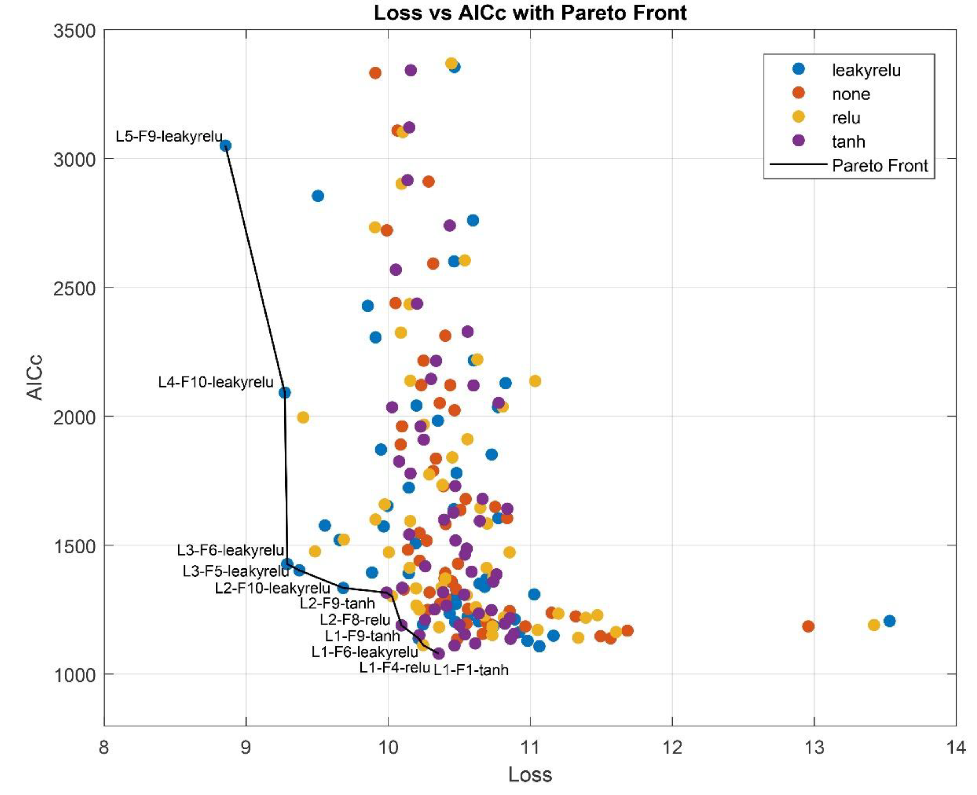
In the second step, the scope of the parameter search was narrowed to focus on the activation function (ReLU, Leaky ReLU, Tanh, or none), the number of LSTM hidden units (ranging from 1 to 5), and the number of fully connected layer nodes (ranging from 1 to 10). The upper limit for LSTM hidden units was intentionally kept low to prevent overparameterization, as each additional LSTM unit substantially increases the total number of trainable parameters. In contrast, the number of FC layer nodes was expanded up to 10 based on favorable results observed in the previous optimization step, where larger FC layers contributed to improved model performance without incurring excessive computational cost. With only 200 possible combinations, a full grid search was conducted during the second screening step. Each network architecture was evaluated across 10 training runs, and only the best-performing candidate was retained for each parameter combination. To balance validation loss with model complexity and mitigate overparameterization, a loss vs. AICc plot was generated to identify the Pareto front (Figure A1). From this front, five network architectures that best balanced low validation loss and favorable AICc values were selected for further evaluation.
In the third step, the selected models were trained in full for 20,000 iterations, and their predictive performance was assessed using validation loss. The best-performing model was chosen as the optimal network configuration for the specific hybrid process model. Finally, the impact of incorporating a dropout layer within the finalized hybrid model architecture was thoroughly investigated to assess its effect on model robustness and generalization performance.
Hybrid model transfer learning
To leverage the selected trained hybrid model for a new experimental dataset involving Qβ production, a transfer learning approach was applied. The previously optimized model architecture, trained on the historical dataset, served as the starting point. All model weights were initialized from this pre-trained network to retain learned temporal and process dynamics. To adapt the model to the Qβ dataset, only the final fully connected layer was unfrozen and fine-tuned using the new data, while the LSTM unit—capturing general process behavior—was kept fixed. This strategy allows the model to efficiently adapt to the specific characteristics of the Qβ process while preserving useful generalizations from the original training, thereby reducing training time and improving predictive accuracy with limited new data. Experiment 20 was used for testing loss calculation.
Model Predictive Control (MPC) architecture
A comprehensive model predictive control framework was developed and implemented, leveraging the advanced hybrid process model. The main task of the MPC controller was to track a pre-selected growth trajectory close to the maximum specific growth rate of the cells.
The MPC algorithm was implemented to dynamically estimate the optimal substrate feed rate, Fₛ(t), required to maintain a desired specific growth rate, μₛₑₜ(t). In the developed hybrid modeling framework, the substrate feed rate served as an input, while the specific growth rate was one of the predicted outputs. Due to the non-invertible structure of the hybrid model, analytical inversion to compute Fₛ(t) from a given μₛₑₜ(t) was not feasible. Consequently, a numerical optimization approach was employed at each control step using MATLAB’s bounded nonlinear optimization function fminbnd, which searched for the optimal feed rate within specified operational constraints. The optimization problem at each time step was formulated as:
subject to the hybrid model dynamics:
where x(k) is the vector of the state variables, and μ(k) is the predicted specific growth rate at step k. The control horizon was set to Nc = 1 hour and the prediction horizon to Np = 12 hours. The hybrid model itself was simulated with a finer sampling time of 1 minute to ensure accurate forward predictions, while the MPC made decisions on an hourly basis.
To improve model accuracy and adaptability, the hybrid model was retrained after each sampling (approx. three times per day). Each time, the newly measured biomass concentration, Xmeas(t), was appended to the training dataset, and the model parameters were updated to reflect the latest process dynamics.
The MPC framework was experimentally validated in a P. pastoris fed-batch fermentation under the methanol-inducible AOX1 promoter. Real-time process data, including substrate feed rate, base and antifoam addition, were integrated into MATLAB via an OPC server, enabling seamless bidirectional communication with the SCADA system. A more technical description is available elsewhere [33]. This real-time data integration allowed the MPC to adjust the substrate feed rate based on actual process conditions.
MPC was initiated after methanol adaptation, typically 8–10 hours after inoculation. The growth rate setpoint μₛₑₜ(t) was scheduled in a step-wise fashion to reflect the physiological limits of the cells: an initial value of 0.04 h⁻¹ was maintained for the first 12 hours, followed by reductions to 0.02 h⁻¹ and 0.01 h⁻¹ at 12-hour intervals. This trajectory was selected to optimize productivity while preventing metabolic overload during prolonged methanol feeding.
3. Results
3.1. Optimal hybrid model architecture screening
The Bayesian optimization approach was effectively employed to identify optimal hybrid model architectures. Although not all configurations within the design space were explored, the method yielded valuable insights while substantially narrowing the range of candidate architectures. This efficiency stems from the Bayesian framework’s ability to prioritize promising regions of the hyperparameter space, reducing the number of models requiring evaluation. The ten best-performing network architectures, ranked by their validation loss, are summarized in Table 2.
The results of the Bayesian optimization screening indicate that while individual performance metrics varied across architectures, consistent structural trends emerged among the top-performing models. Notably, all ten selected architectures include an LSTM layer as the first hidden layer, emphasizing the importance of temporal feature extraction in capturing the dynamics of the process. This is followed in each case by at least one fully connected layer, which likely contributes to nonlinear transformation and mapping of the LSTM outputs to the target outputs. This consistent architectural pattern suggests that the hybrid model benefits from a sequence-aware representation (via LSTM), followed by flexible function approximation (via FC layers). Although the activation functions and number of units varied, these two structural components formed the core of the most effective configurations, reinforcing their critical role in model performance.
In the subsequent step, a comprehensive grid search was conducted across the full domain of feasible network architectures to investigate the optimal number of hidden units, node counts, and activation functions for the hidden layers. This systematic approach enabled an exhaustive evaluation of all combinations of relevant hyperparameters, ensuring that no potentially optimal configuration within the predefined design space was overlooked. To mitigate the risk of network overparameterization, AICc values were evaluated in parallel with validation loss. Candidate architectures from the Pareto front of the Loss vs. AICc plot (Figure A1) were identified as the most promising, and their configurations are detailed in Table 3.
To ensure a balanced trade-off between predictive accuracy and model complexity, the middle five architectures from the Pareto front were selected for further optimization. These architectures, indicated with an asterisk in Table 3, offer a pragmatic compromise: they demonstrate competitive validation losses (ranging from 9.37% to 10.26%) while maintaining a relatively low number of trainable parameters (between 76 and 146). This subset effectively spans the central region of the Pareto front, avoiding both the highly complex models at the top—which, despite slightly better accuracy, incur significantly higher parameter counts and AICc values—and the simplest models at the bottom, which show diminishing returns in terms of validation loss. By focusing on this middle range, the selected architectures are expected to generalize well while remaining computationally efficient and less prone to overfitting.
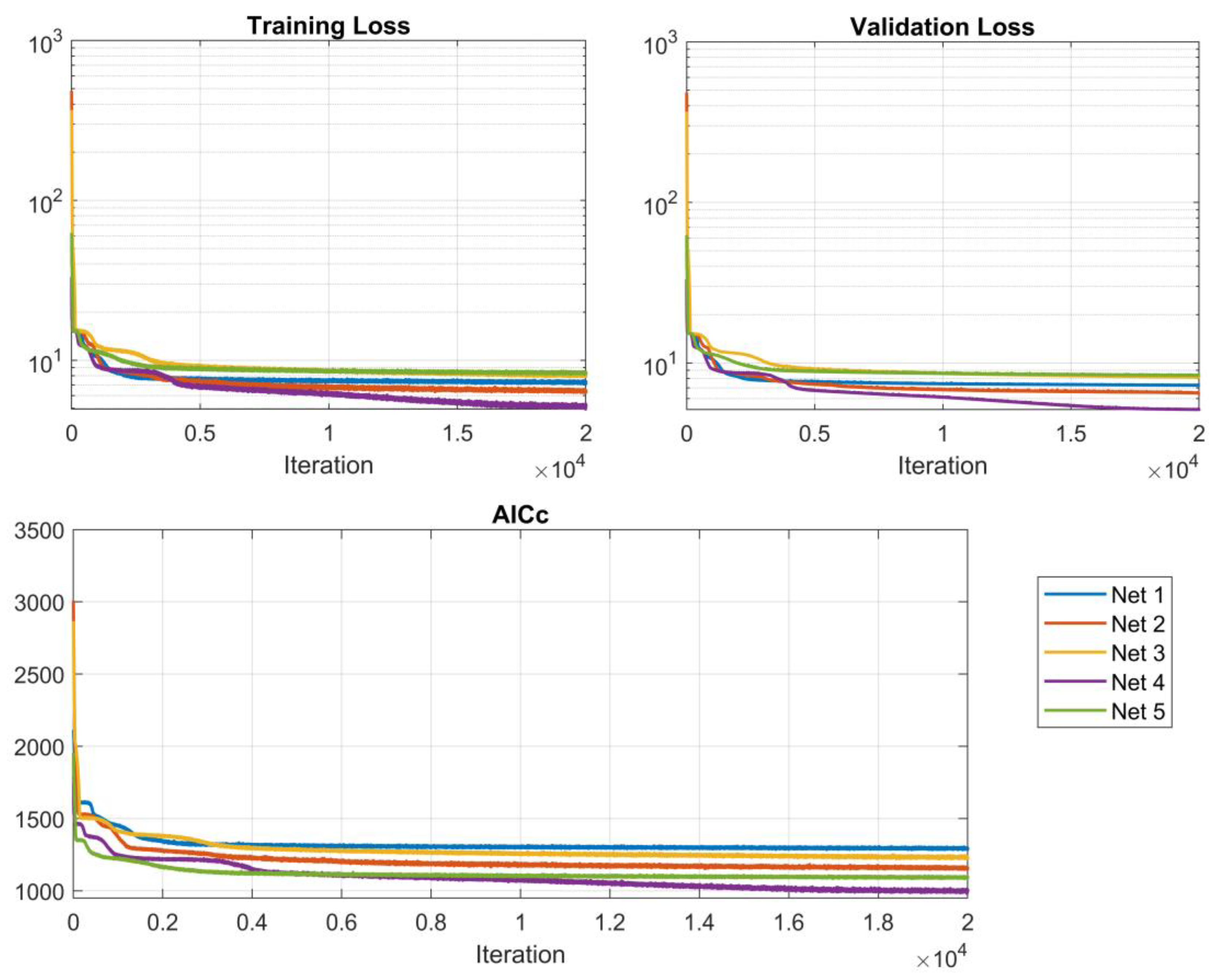
In the final step, the five selected network architectures underwent an extensive evaluation to rigorously assess their stability and predictive performance. Each architecture was trained independently across 10 separate runs, with each training session lasting 20,000 iterations. This repeated training procedure helped account for variability due to random initialization and stochastic optimization effects, ensuring a robust comparison of model reliability and convergence behavior. The results, including key performance metrics such as validation loss and generalization capability, from every network’s best session, are summarized in Table 4.
Training results indicate that the optimal network architecture comprises 2 hidden units in the LSTM layer, 8 fully connected layer nodes, and utilizes a ReLU activation function. This configuration achieved the best performance, with a validation loss of 4.93% and the lowest AICc value of 998 among all evaluated models, demonstrating an excellent balance between predictive accuracy and model complexity. The training graphs are shown in Figure 2.
Figure 2.
Training plots for the 5 best-performing network architectures.
The inclusion of a dropout layer with varying probabilities (ranging from 0.1 to 0.5) was systematically evaluated. The results showed that increasing the dropout rate consistently led to higher validation losses. Even a modest dropout probability of 0.1 negatively impacted model performance, suggesting that the selected network architecture is already sufficiently regularized and relatively simple. In such cases, the additional noise introduced by dropout appears to hinder learning rather than mitigate overfitting. This outcome implies that the model generalizes well without further regularization, and applying dropout may introduce unnecessary instability or lead to underfitting. Moreover, the observation may reflect the nature of the dataset, which is likely clean and of limited size—conditions under which every training instance is valuable and even minimal information loss (through activation masking) can reduce training efficiency.
3.2. Adapting the hybrid model to Qβ dataset with Transfer Learning
Finally, the already trained optimal hybrid model was adapted to the new dataset (Qβ fermentations) using transfer learning. The LSTM layer weights were frozen, allowing the network to retain useful generalizations from the original training.
The resulting network demonstrated strong predictive performance, achieving a training loss of 3.18%, a validation loss of 3.53%, and a testing loss of 5.61%. Additionally, the corrected AICc value was 856, reflecting a favorable balance between model complexity and goodness of fit. Together, these metrics indicate that the hybrid model effectively captured the underlying dynamics of the experimental dataset while maintaining generalization to unseen data (Figure 3).
As illustrated in Figure 3, the hybrid model demonstrated strong predictive capability by closely capturing the dynamic behavior of the modeled variables throughout the fermentation process. Quantitatively, the model achieved a NRMSE of 1.68% for biomass concentration (X), indicating high accuracy in cell growth prediction, and 9.54% for product concentration (P), reflecting reliable estimation of recombinant protein production.
3.3. Hybrid MPC experimental validation
To evaluate the practical applicability and effectiveness of the hybrid MPC framework, experimental validation was carried out controlling the feed rate in an actual fermentation run. This allowed for assessment of the system’s ability to predict and regulate key bioprocess variables in real-time. The results can be seen in Figure 4.
The tracking accuracy of cell biomass (X) by the hybrid model can be characterized as moderate. Notably, the model failed to adequately capture the physiological adaptation phase of P. pastoris to methanol during the first 8–12 hours following induction—a period in which cellular growth is minimal or absent. As a result, predictions during this early phase were consistently higher than observed values. In the later stages of fermentation, the model exhibited a tendency to overestimate biomass concentration. To compensate for this discrepancy, manual adjustments to the biomass profile were introduced during model re-training, following the availability of offline sampling data. Despite these limitations, the model achieved an overall NRMSE of 6.51% for biomass prediction, indicating acceptable predictive performance.
With respect to product concentration (P), the model similarly demonstrated a tendency to overestimate values across the fermentation timeline. This resulted in an average NRMSE of 14.65%, suggesting moderate accuracy in modeling recombinant protein production dynamics.
Although the predictive accuracy of the model was not exemplary—particularly in tracking certain state variables with high precision—it nonetheless demonstrated strong performance in its control functionality. Specifically, the model was able to generate robust and reliable feed rate profiles, effectively regulating substrate addition to maintain the desired specific growth rate throughout the fermentation process. This highlights the strength of the hybrid MPC framework in achieving process objectives, even in the presence of moderate prediction errors. The µ tracking results are presented in Figure 5.
The hybrid MPC system demonstrated good performance in tracking the specific growth rate set-point over the course of the fermentation. However, similar to the behavior observed in the prediction model, a slight deviation from the target biomass trajectory was noted during the final 12 hours of the process—particularly after the specific growth rate was reduced to 0.001 h-1. This deviation is likely attributable to the cytotoxic effects of methanol accumulation, which can impair cellular metabolism and inhibit biomass formation in the later stages of fermentation. This phenomenon is further reflected in the growth rate tracking plot, where the measured specific growth rate was consistently lower than the target value during this terminal phase.
Overall, while minor discrepancies emerged toward the end of the process, the control system maintained a high degree of accuracy in regulating growth for the majority of the fermentation, underscoring its effectiveness and reliability under realistic bioprocessing conditions.
4. Discussion
This study highlights the efficiency of Bayesian optimization in identifying high-performing hybrid neural network architectures for dynamic bioprocess modeling. By concentrating on the most promising regions of the hyperparameter space, as demonstrated in neural architecture search literature [53], Bayesian optimization substantially reduces the number of candidate configurations compared to exhaustive strategies like grid or random search. A consistent architectural pattern emerged among the top models: an LSTM layer followed by one or more fully connected (FC) layers. This aligns with findings that temporal feature extraction via LSTM is critical in sequence modeling, especially in bioprocess contexts [54]. The FC layers then effectively map these temporal representations into nonlinear predictive outputs.
The grid search extended this exploration and employed AICc alongside validation loss to avoid overfitting. This Pareto front strategy is known to balance model complexity and accuracy [31]. Selecting architectures from the mid-section of the Pareto front ensured efficient, generalizable models without unnecessary computational burden.
Robustness was confirmed through repeated training of the selected architectures, mitigating variability from random initialization. The best-performing model—a minimal architecture with 2 LSTM units and 8 FC nodes—achieved the lowest validation loss and AICc, illustrating that compact models can deliver strong performance. This has practical implications for real-time applications, where computational efficiency and stability are critical. Interestingly, dropout regularization consistently worsened performance, in contrast to its typical use in neural networks [55]. This suggests that for relatively clean and small datasets, additional noise can lead to underfitting rather than preventing overfitting, corroborating findings in Bayesian LSTM studies [56].
In summary, the structured workflow—combining Bayesian optimization, exhaustive grid search, and performance validation—successfully identified robust and efficient hybrid models. These findings offer valuable guidance for developing data-driven models in bioprocessing, particularly where data is limited and interpretability and computational efficiency are priorities.
The application of transfer learning significantly enhanced predictive modeling in Qβ fermentation. By freezing the pretrained LSTM layer, the model effectively retained temporal feature representations learned from the original fermentation dataset—an approach aligned with known benefits of sequential inductive transfer learning, where pretrained layers serve as robust feature extractors.
Performance metrics indicate robust predictive capability: training loss of 3.18%, validation loss of 3.53%, and testing loss of 5.61%, alongside an AICc value of 856. These figures suggest the model strikes a favorable balance between complexity and fit, as AICc penalizes excessive parameters. Figure 3 illustrates that the hybrid model accurately tracks the dynamic behavior of key process variables throughout the fermentation. Notably, the NRMSE of 1.68% for biomass (X) reflects excellent predictive accuracy, while a 9.54% NRMSE for product concentration (P) indicates reliable estimation of recombinant protein output—performance consistent with successful domain adaptation observed in bioprocess transfer learning studies.
Overall, these results highlight that freezing the LSTM backbone preserves essential time-series features, enabling efficient adaptation to new but related bioprocesses. This echoes broader evidence that transfer learning, particularly with LSTM architectures, reliably enhances performance in data-constrained scenarios [27]. The Qβ model's strong performance, with an experimental dataset of only 3 fermentation runs, underscores the hybrid model's generalizability, positioning this approach as a promising strategy for rapid deployment in diverse fermentation contexts.
To assess the practical utility of the hybrid MPC framework, a real-time control experiment was conducted involving feed rate adjustment in an actual P. pastoris fermentation (Figure 4). This exercise evaluated the framework’s ability to predict and regulate critical bioprocess variables during active operation. The hybrid model achieved a biomass NRMSE of 6.51%, indicative of moderate accuracy. However, the model struggled during the 8–12 hour adaptation phase following methanol induction, consistently overestimating X—likely due to the challenge of capturing initial physiological delays. During later stages, persistent biomass overestimation required offline-informed manual corrections, a common issue in MPC applications where adaptation lags affect real-time feedback control. Again, the model tended to overpredict P, with an average NRMSE of 14.65%, revealing moderate accuracy in tracking recombinant protein dynamics.
Despite prediction inaccuracies, the hybrid MPC effectively maintained the target specific growth rate (µ) via robust feed profiles (Figure 5). This demonstrates the framework’s resilience and ability to meet control objectives even under prediction uncertainty. However, in the final 12 hours—particularly after µ dropped to 0.001 h⁻¹—deviations emerged. These were likely driven by methanol-induced cytotoxicity, which reduced cellular metabolism and hindered biomass formation.
The hybrid MPC system showed strong real-time control capabilities, effectively regulating substrate feed to meet specific growth objectives throughout most of the fermentation. Prediction errors were manageable and did not significantly impair overall control performance. The observed late-stage deviations underscore the importance of incorporating biological stress factors—such as methanol toxicity—into model formulations.
This validation confirms that hybrid MPC, built on data-driven hybrid models, is a viable strategy for real-world bioprocess control. Future work should focus on refining model representations—possibly by including toxicity effects—and improving early-stage adaptation dynamics. Doing so would further enhance both predictive fidelity and control reliability, supporting broader application in fermentation-based production workflows. Also, a reliable estimator for recombinant protein concentration should be included in the MPC framework to provide accurate and reliable estimations to use for hybrid model re-training during operation.
5. Conclusions
This study presents a comprehensive framework for hybrid modeling and control of P. pastoris fed-batch fermentations, integrating deep learning with model predictive control (MPC). The use of Bayesian optimization proved effective in identifying efficient and accurate hybrid neural network architectures, with consistent structural trends—namely, the inclusion of an LSTM layer followed by fully connected layers—emerging among top-performing models. A complementary grid search, guided by AICc and validation loss, enabled the selection of models that balance accuracy with computational simplicity.
Transfer learning was successfully employed to adapt the optimal hybrid model to Qβ fermentation data, achieving strong predictive performance while preserving generalizable temporal features. This highlights the model's flexibility and potential for rapid adaptation to new, yet related, bioprocesses—an important capability in multiproduct biomanufacturing environments.
Experimental validation of the hybrid MPC framework demonstrated reliable real-time control of the fermentation process, despite moderate prediction errors in biomass and product concentration. Notably, the system maintained accurate regulation of the specific growth rate throughout most of the process, underscoring its practical robustness.
In summary, this work establishes a robust, adaptable, and computationally efficient hybrid modeling approach for model predictive bioprocess control. The combination of automated architecture search, transfer learning, and MPC provides a scalable methodology for accelerating digital twin deployment in industrial biotechnology. Future work should aim to enhance biological realism and expand generalizability across strains and production conditions.
Author Contributions
Conceptualization, E.B., V.G. and A.K.; methodology, E.B., V.G. and A.K.; software, E.B.; validation, E.B..; formal analysis, E.B.; investigation, E.B. and O.G.; resources, A.K.; data curation, E.B.; writing—original draft preparation, E.B.; writing—review and editing, E.B, V.G., A.K., O.G. and J.V.; visualization, E.B.; supervision, V.G. and A.K.; project administration, E.B. and J.V.; funding acquisition, J.V. and A.K. All authors have read and agreed to the published version of the manuscript.
Funding
This research was funded by the EU Recovery and Resilience Facility within Project No 5.2.1.1.i.0/2/24/I/CFLA/003 “Implementation of consolidation and management changes at Riga Technical University, Liepaja University, Rezekne Academy of Technology, Latvian Maritime Academy and Liepaja Maritime College for the progress towards excellence in higher education, science and innovation” academic career doctoral grant No. 1094.
Data Availability Statement
The datasets presented in this article are not readily available because the data are part of an ongoing study. Requests to access the datasets should be directed to E. Bolmanis.
Acknowledgments
We acknowledge Riga Technical University’s HPC Center for providing access to their computing infrastructure. The authors would also like to acknowledge the contribution of Inara Akopjana for preparing seed inoculation cultures and performing SDS-PAGE analysis, and Janis Bogans for performing chromatography runs.
Conflicts of Interest
The authors declare no conflicts of interest.
Appendix A
Figure A1.
Pareto front, demonstrating the best model architectures, considering Loss and AICc. L stands for LSTM layer hidden units, F – for FC hidden nodes, followed by activation function. For example, L4-F10-leakyrelu is an LSTM layer with 4 hidden units, followed by a FC layer with 10 nodes and leaky relu activation.
References
- Bailey, J.E. Mathematical Modeling and Analysis in Biochemical Engineering: Past Accomplishments and Future Opportunities. Biotechnol Prog 1998, 14, 8–20. [Google Scholar] [CrossRef] [PubMed]
- Noll, P.; Henkel, M. History and Evolution of Modeling in Biotechnology: Modeling & Simulation, Application and Hardware Performance. Comput Struct Biotechnol J 2020, 18, 3309–3323. [Google Scholar] [CrossRef]
- Heinemann, M.; Panke, S. Synthetic Biology - Putting Engineering into Biology. Bioinformatics 2006, 22, 2790–2799. [Google Scholar] [CrossRef] [PubMed]
- Lee, J.; Kao, H.-A.; Bagheri, B. Recent Advances and Trends of Cyber-Physical Systems and Big Data Analytics in Industrial Informatics. Proceeding of Int. Conference on Industrial Informatics (INDIN). Porto Alegre, Brazil, July 2014. [CrossRef]
- Agharafeie, R.; Ramos, J.R.C.; Mendes, J.M.; Oliveira, R. From Shallow to Deep Bioprocess Hybrid Modeling: Advances and Future Perspectives. Fermentation 2023, 9, 1–22. [Google Scholar] [CrossRef]
- Carbonell, P.; Radivojevic, T.; García Martín, H. Opportunities at the Intersection of Synthetic Biology, Machine Learning, and Automation. ACS Synth Biol 2019, 8, 1474–1477. [Google Scholar] [CrossRef] [PubMed]
- Glassey, J.; Gernaey, K. V.; Clemens, C.; Schulz, T.W.; Oliveira, R.; Striedner, G.; Mandenius, C.F. Process Analytical Technology (PAT) for Biopharmaceuticals. Biotechnol J 2011, 6, 369–377. [Google Scholar] [CrossRef]
- Sun, Y.; Nathan-Roberts, W.; Pham, T.D.; Otte, E.; Aickelin, U. Multi-Fidelity Gaussian Process for Biomanufacturing Process Modeling with Small Data. arXiv 2022, arXiv:2211.14493. [Google Scholar]
- Pinto, J.; Ramos, J.R.C.; Costa, R.S.; Oliveira, R. Hybrid Deep Modeling of a GS115 (Mut+) Pichia Pastoris Culture with State–Space Reduction. Fermentation 2023, 9. [Google Scholar] [CrossRef]
- Pinto, J.; Mestre, M.; Ramos, J.; Costa, R.S.; Striedner, G.; Oliveira, R. A General Deep Hybrid Model for Bioreactor Systems: Combining First Principles with Deep Neural Networks. Comput Chem Eng 2022, 165, 107952. [Google Scholar] [CrossRef]
- Ramos, J.R.C.; Pinto, J.; Poiares-Oliveira, G.; Peeters, L.; Dumas, P.; Oliveira, R. Deep Hybrid Modeling of a HEK293 Process: Combining Long Short-Term Memory Networks with First Principles Equations. Biotechnol Bioeng 2024, 121, 1554–1568. [Google Scholar] [CrossRef]
- Ferreira, A.R.; Dias, J.M.L.; Von Stosch, M.; Clemente, J.; Cunha, A.E.; Oliveira, R. Fast Development of Pichia Pastoris GS115 Mut+ Cultures Employing Batch-to-Batch Control and Hybrid Semi-Parametric Modeling. Bioprocess Biosyst Eng 2014, 37, 629–639. [Google Scholar] [CrossRef] [PubMed]
- Narayanan, H.; von Stosch, M.; Feidl, F.; Sokolov, M.; Morbidelli, M.; Butté, A. Hybrid Modeling for Biopharmaceutical Processes: Advantages, Opportunities, and Implementation. Front chem eng 2023, 5. [Google Scholar] [CrossRef]
- Schweidtmann, A.M.; Zhang, D.; von Stosch, M. A Review and Perspective on Hybrid Modeling Methodologies. Digit Chem Eng 2024, 10, 100136. [Google Scholar] [CrossRef]
- von Stosch, M.; Oliveira, R.; Peres, J.; Feyo de Azevedo, S. Hybrid Semi-Parametric Modeling in Process Systems Engineering: Past, Present and Future. Comput Chem Eng 2014, 60, 86–101. [Google Scholar] [CrossRef]
- Psichogios, D.C.; Ungar, L.H. A Hybrid Neural Network-First Principles Approach to Process Modeling. AIChE J. 1992, 38, 1499–1511. [Google Scholar] [CrossRef]
- von Stosch, M.; Davy, S.; Francois, K.; Galvanauskas, V.; Hamelink, J.M.; Luebbert, A.; Mayer, M.; Oliveira, R.; O’Kennedy, R.; Rice, P.; et al. Hybrid Modeling for Quality by Design and PAT-Benefits and Challenges of Applications in Biopharmaceutical Industry. Biotechnol J 2014, 9, 719–726. [Google Scholar] [CrossRef]
- Mhaskar, H.N.; Poggio, T. Deep vs. Shallow Networks: An Approximation Theory Perspective. Anal Appl 2016, 14, 829–848. [Google Scholar] [CrossRef]
- Lecun, Y.; Bengio, Y.; Hinton, G. Deep Learning. Nature 2015, 521, 436–444. [Google Scholar] [CrossRef]
- Kingma, D.P.; Ba, J. Adam: A Method for Stochastic Optimization. arXiv 2014, arXiv:1412.6980. [Google Scholar]
- Helleckes, L.M.; Hemmerich, J.; Wiechert, W.; von Lieres, E.; Grünberger, A. Machine Learning in Bioprocess Development: From Promise to Practice. Trends Biotechnol 2023, 41, 817–835. [Google Scholar] [CrossRef]
- Alzubaidi, L.; Bai, J.; Al-Sabaawi, A.; Santamaría, J.; Albahri, A.S.; Al-dabbagh, B.S.N.; Fadhel, M.A.; Manoufali, M.; Zhang, J.; Al-Timemy, A.H.; et al. A Survey on Deep Learning Tools Dealing with Data Scarcity: Definitions, Challenges, Solutions, Tips, and Applications. J Big Data 2023, 10. [Google Scholar] [CrossRef]
- How Invert uses meta-learning to leverage old bioprocess data. Available online: https://invertbio.com/blogs/how-invert-uses-meta-learning-to-leverage-old-data-and-make-better-biomanufacturing-predictions (accessed on 25 June 2025).
- Duong-Trung, N.; Born, S.; Kim, J.W.; Schermeyer, M.-T.; Paulick, K.; Borisyak, M.; Cruz-Bournazou, M.N.; Werner, T.; Scholz, R.; Schmidt-Thieme, L.; et al. When Bioprocess Engineering Meets Machine Learning: A Survey from the Perspective of Automated Bioprocess Development. Biochem Eng J 2022, 190, 108764. [Google Scholar] [CrossRef]
- Pan, S.J.; Yang, Q. A Survey on Transfer Learning. IEEE Trans Knowl Data Eng 2010, 22, 1345–1359. [Google Scholar] [CrossRef]
- Weiss, K.; Khoshgoftaar, T.M.; Wang, D.D. A Survey of Transfer Learning. J Big Data 2016, 3. [Google Scholar] [CrossRef]
- Rogers, A.W.; Vega-Ramon, F.; Yan, J.; del Río-Chanona, E.A.; Jing, K.; Zhang, D. A Transfer Learning Approach for Predictive Modeling of Bioprocesses Using Small Data. Biotechnol Bioeng 2022, 119, 411–422. [Google Scholar] [CrossRef]
- Kensert, A.; Harrison, P.J.; Spjuth, O. Transfer Learning with Deep Convolutional Neural Networks for Classifying Cellular Morphological Changes. SLAS Discov 2019, 24, 466–475. [Google Scholar] [CrossRef] [PubMed]
- Iman, M.; Rasheed, K.; Arabnia, H.R. A Review of Deep Transfer Learning and Recent Advancements. Technologies 2022, 11. [Google Scholar] [CrossRef]
- Narayanan, H.; Luna, M.; Sokolov, M.; Butté, A.; Morbidelli, M. Hybrid Models Based on Machine Learning and an Increasing Degree of Process Knowledge: Application to Cell Culture Processes. Ind Eng Chem Res 2022, 61, 8658–8672. [Google Scholar] [CrossRef]
- Liashchynskyi, P.; Liashchynskyi, P. Grid Search, Random Search, Genetic Algorithm: A Big Comparison for NAS, arXiv 2019. arXiv:1912.06059v1.
- Snoek, J.; Larochelle, H.; Adams, R.P. Practical Bayesian Optimization of Machine Learning Algorithms, arXiv 2012. arXiv:1206.2944.
- Bolmanis, E.; Dubencovs, K.; Suleiko, A.; Vanags, J. Model Predictive Control—A Stand Out among Competitors for Fed-Batch Fermentation Improvement. Fermentation 2023, 9, 206. [Google Scholar] [CrossRef]
- Mears, L.; Stocks, S.M.; Sin, G.; Gernaey, K. V. A Review of Control Strategies for Manipulating the Feed Rate in Fed-Batch Fermentation Processes. J Biotechnol 2017, 245, 34–46. [Google Scholar] [CrossRef]
- Rashedi, M.; Khodabandehlou, H.; Demers, M.; Wang, T.; Garvin, C. Model Predictive Controller Design for Bioprocesses Based on Machine Learning Algorithms. In Proceedings of the 13th IFAC Symposium on Dynamics and Control of Process Systems, including Biosystems DYCOPS 2022, Busan, Republic of Korea, 14–17 June 2022; 45–50. [Google Scholar] [CrossRef]
- Eslami, T.; Jungbauer, A. Control Strategy for Biopharmaceutical Production by Model Predictive Control. Biotechnol Prog 2024, 40, 1–19. [Google Scholar] [CrossRef]
- Lyubenova, V.; Ignatova, M.; Zoteva, D.; Roeva, O. Model-Based Adaptive Control of Bioreactors—A Brief Review. Mathematics 2024, 12. [Google Scholar] [CrossRef]
- Mahanty, B. Hybrid Modeling in Bioprocess Dynamics: Structural Variabilities, Implementation Strategies, and Practical Challenges. Biotechnol Bioeng 2023, 120, 2072–2091. [Google Scholar] [CrossRef] [PubMed]
- De Jong, H.; Casagranda, S.; Giordano, N.; Cinquemani, E.; Ropers, D.; Geiselmann, J.; Gouzé, J.L. Mathematical Modelling of Microbes: Metabolism, Gene Expression and Growth. J R Soc Interface 2017, 14. [Google Scholar] [CrossRef] [PubMed]
- Tsopanoglou, A.; Jiménez del Val, I. Moving towards an Era of Hybrid Modelling: Advantages and Challenges of Coupling Mechanistic and Data-Driven Models for Upstream Pharmaceutical Bioprocesses. Curr Opin Chem Eng 2021, 32. [Google Scholar] [CrossRef]
- Galvanauskas, V.; Simutis, R.; Lübbert, A. Hybrid Modeling of Biochemical Processes. In Hybrid Modeling in Process Industries, 1st ed.; Glassey, J., von Stosch, M., Eds.; CRC Press: Boca Raton, USA, 2018; pp. 89–127. [Google Scholar]
- Cregg, J.M.; Cereghino, J.L.; Shi, J.; Higgins, D.R. Recombinant Protein Expression in Pichia Pastoris. Mol Biotechnol 2000, 16, 23–52. [Google Scholar] [CrossRef] [PubMed]
- Macauley-Patrick, S.; Fazenda, M.L.; McNeil, B.; Harvey, L.M. Heterologous Protein Production Using the Pichia Pastoris Expression System. Yeast 2005, 22, 249–270. [Google Scholar] [CrossRef]
- Bolmanis, E.; Grigs, O.; Kazaks, A.; Galvanauskas, V. High-Level Production of Recombinant HBcAg Virus-like Particles in a Mathematically Modelled P. Pastoris GS115 Mut+ Bioreactor Process under Controlled Residual Methanol Concentration. Bioprocess Biosyst Eng 2022, 45, 1447–1463. [Google Scholar] [CrossRef]
- Looser, V.; Bruhlmann, B.; Bumbak, F.; Stenger, C.; Costa, M.; Camattari, A.; Fotiadis, D.; Kovar, K. Cultivation Strategies to Enhance Productivity of Pichia Pastoris: A Review. Biotechnol Adv 2014, 33, 1177–1193. [Google Scholar] [CrossRef]
- Vuitika, L.; Côrtes, N.; Malaquias, V.B.; Silva, J.D.Q.; Lira, A.; Prates-Syed, W.A.; Schimke, L.F.; Luz, D.; Durães-Carvalho, R.; Balan, A.; et al. A Self-Adjuvanted VLPs-Based Covid-19 Vaccine Proven Versatile, Safe, and Highly Protective. Sci Rep 2024, 14. [Google Scholar] [CrossRef]
- Spohn, G.; Keller, I.; Beck, M.; Grest, P.; Jennings, G.T.; Bachmann, M.F. Active Immunization with IL-1 Displayed on Virus-like Particles Protects from Autoimmune Arthritis. Eur J Immunol 2008, 38, 877–887. [Google Scholar] [CrossRef] [PubMed]
- Freivalds, J.; Dislers, A.; Ose, V.; Skrastina, D.; Cielens, I.; Pumpens, P.; Sasnauskas, K.; Kazaks, A. Assembly of Bacteriophage Qβ Virus-like Particles in Yeast Saccharomyces Cerevisiae and Pichia Pastoris. J Biotechnol 2006, 123, 297–303. [Google Scholar] [CrossRef] [PubMed]
- Invitrogen Corporation Pichia Fermentation Process Guidelines. Available online: https://tools.thermofisher.com/content/sfs/manuals/pichiaferm_prot.pdf (accessed on day month year).
- Grigs, O.; Bolmanis, E.; Galvanauskas, V. Application of In-Situ and Soft-Sensors for Estimation of Recombinant P. Pastoris GS115 Biomass Concentration: A Case Analysis of HBcAg (Mut+) and HBsAg (MutS) Production Processes under Varying Conditions. Sensors 2021, 21, 1268. [Google Scholar] [CrossRef] [PubMed]
- Bolmanis, E.; Uhlendorff, S.; Pein-Hackelbusch, M.; Galvanauskas, V.; Grigs, O. Anomaly Detection and Removal Strategies for In-Line Permittivity Sensor Signal Used in Bioprocesses. Front. Bioeng. Biotechnol. 2025. (Article in press).
- Bolmanis, E.; Bogans, J.; Akopjana, I.; Suleiko, A.; Kazaka, T.; Kazaks, A. Production and Purification of Soy Leghemoglobin from Pichia Pastoris Cultivated in Different Expression Media. Processes 2023, 11, 3215. [Google Scholar] [CrossRef]
- White, C.; Ai, A.; Ai, C.; Neiswanger, W.; Savani, Y.; Ai, Y. BANANAS: Bayesian Optimization with Neural Architectures for Neural Architecture Search. arXiv 2020, arXiv:1910.11858. [Google Scholar] [CrossRef]
- Blume, S.; Benedens, T.; Schramm, D. Hyperparameter Optimization Techniques for Designing Software Sensors Based on Artificial Neural Networks. Sensors 2021, 21. [Google Scholar] [CrossRef]
- Gal, Y.; Ghahramani, Z. Dropout as a Bayesian Approximation: Representing Model Uncertainty in Deep Learning. arXiv 2016, arXiv:1506.02142. [Google Scholar]
- Vien, B.S.; Kuen, T.; Rose, L.R.F.; Chiu, W.K. Optimisation and Calibration of Bayesian Neural Network for Probabilistic Prediction of Biogas Performance in an Anaerobic Lagoon. Sensors 2024, 24. [Google Scholar] [CrossRef]
Figure 1.
Overview of the hybrid model structure.
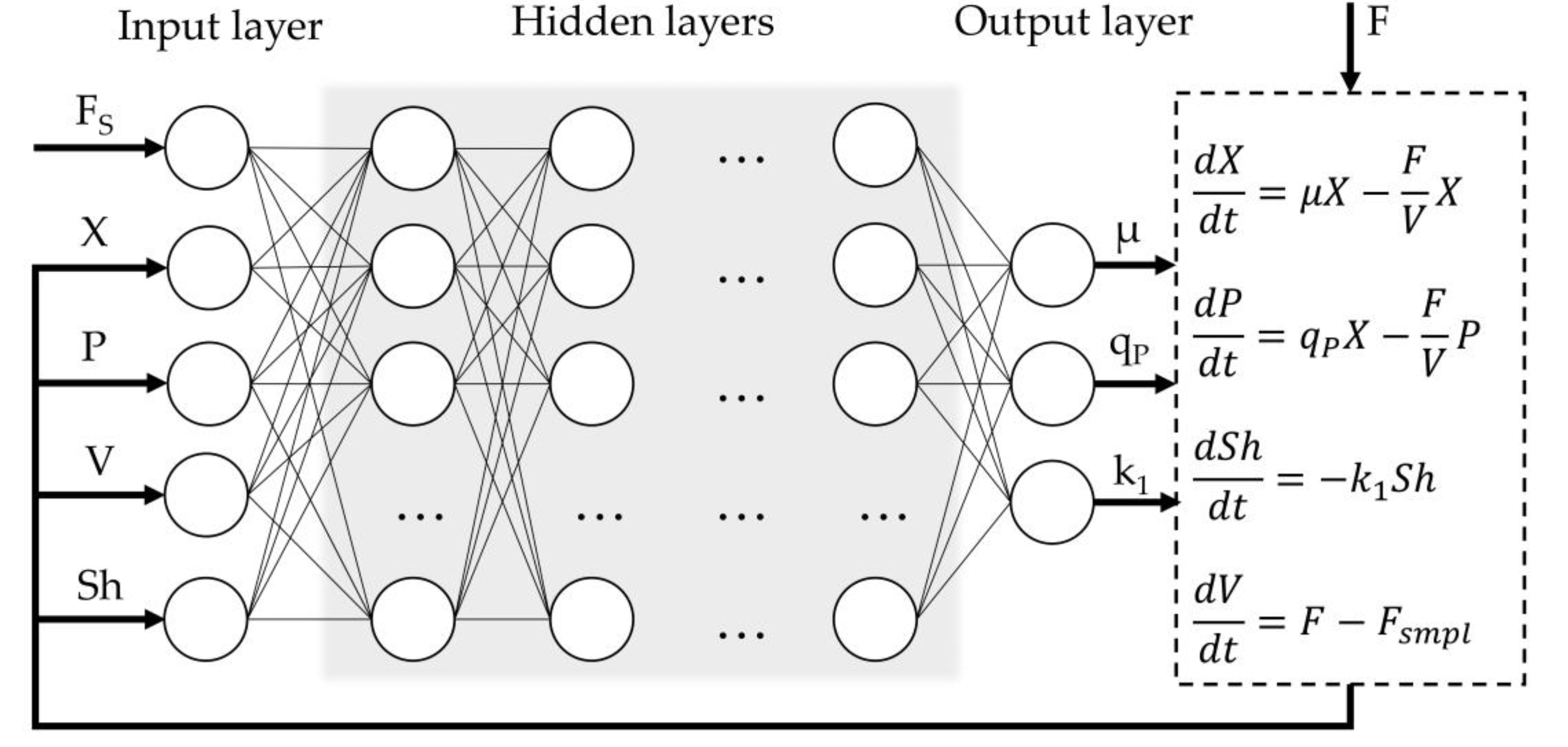
Figure 3.
Prediction of the dynamic profiles of variables (X, P, V, Sh) modeled with the trained hybrid network.
Figure 3.
Prediction of the dynamic profiles of variables (X, P, V, Sh) modeled with the trained hybrid network.
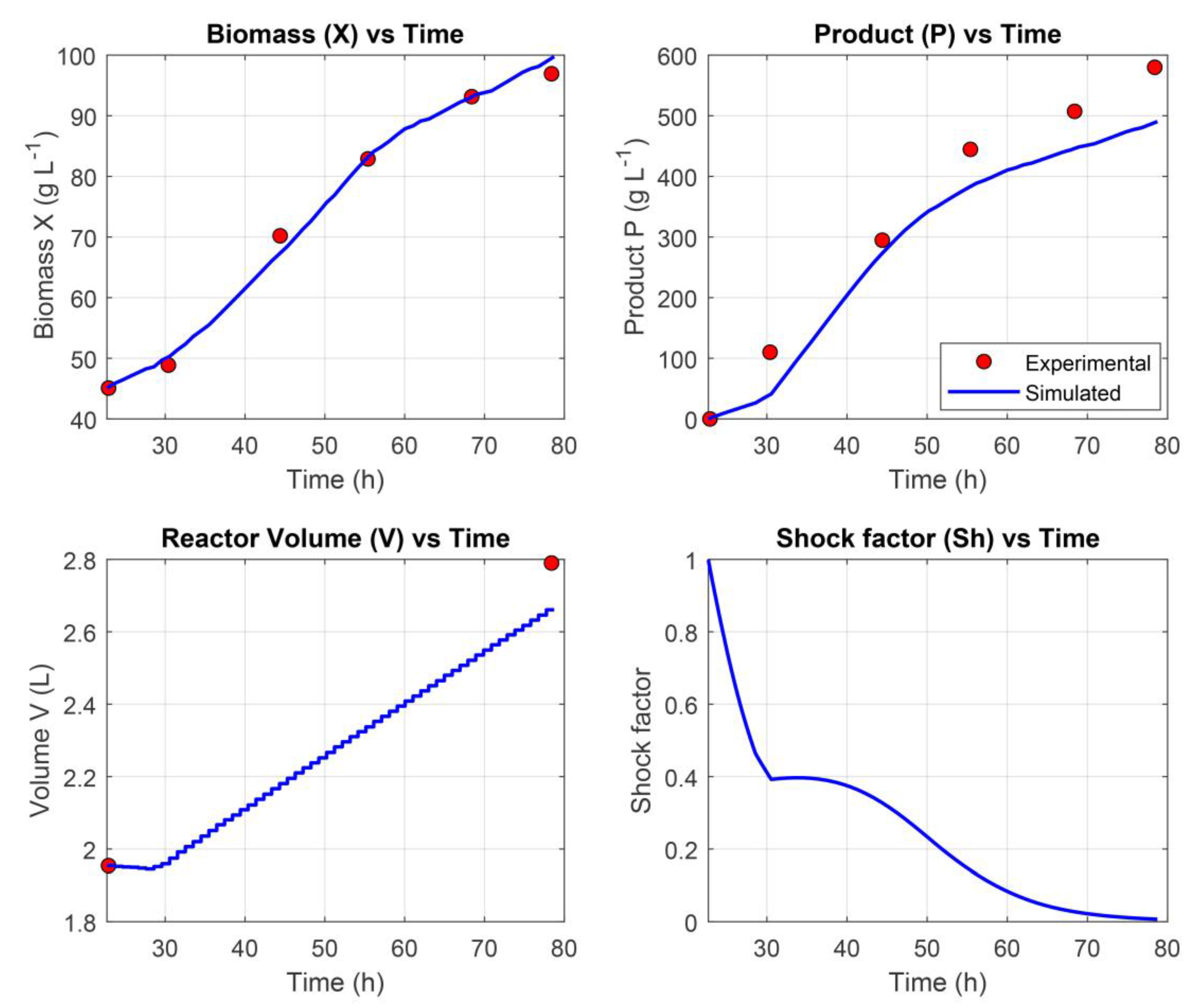
Figure 4.
Hybrid MPC modeling performance during experimental validation.
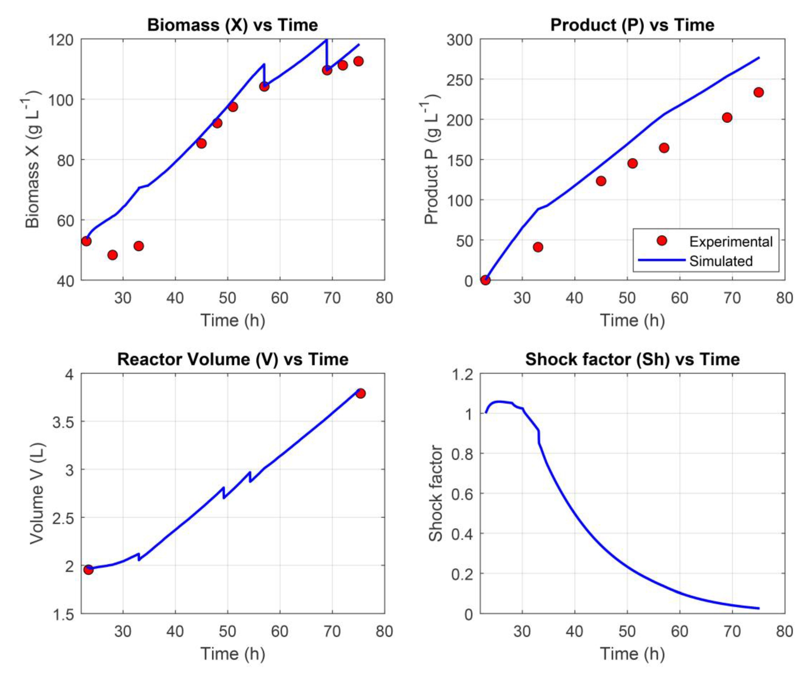
Figure 5.
Target vs experimental biomass growth, specific growth rate and feed rate plots. Vertical lines in the Feed rate plot indicate µ shifts.
Figure 5.
Target vs experimental biomass growth, specific growth rate and feed rate plots. Vertical lines in the Feed rate plot indicate µ shifts.
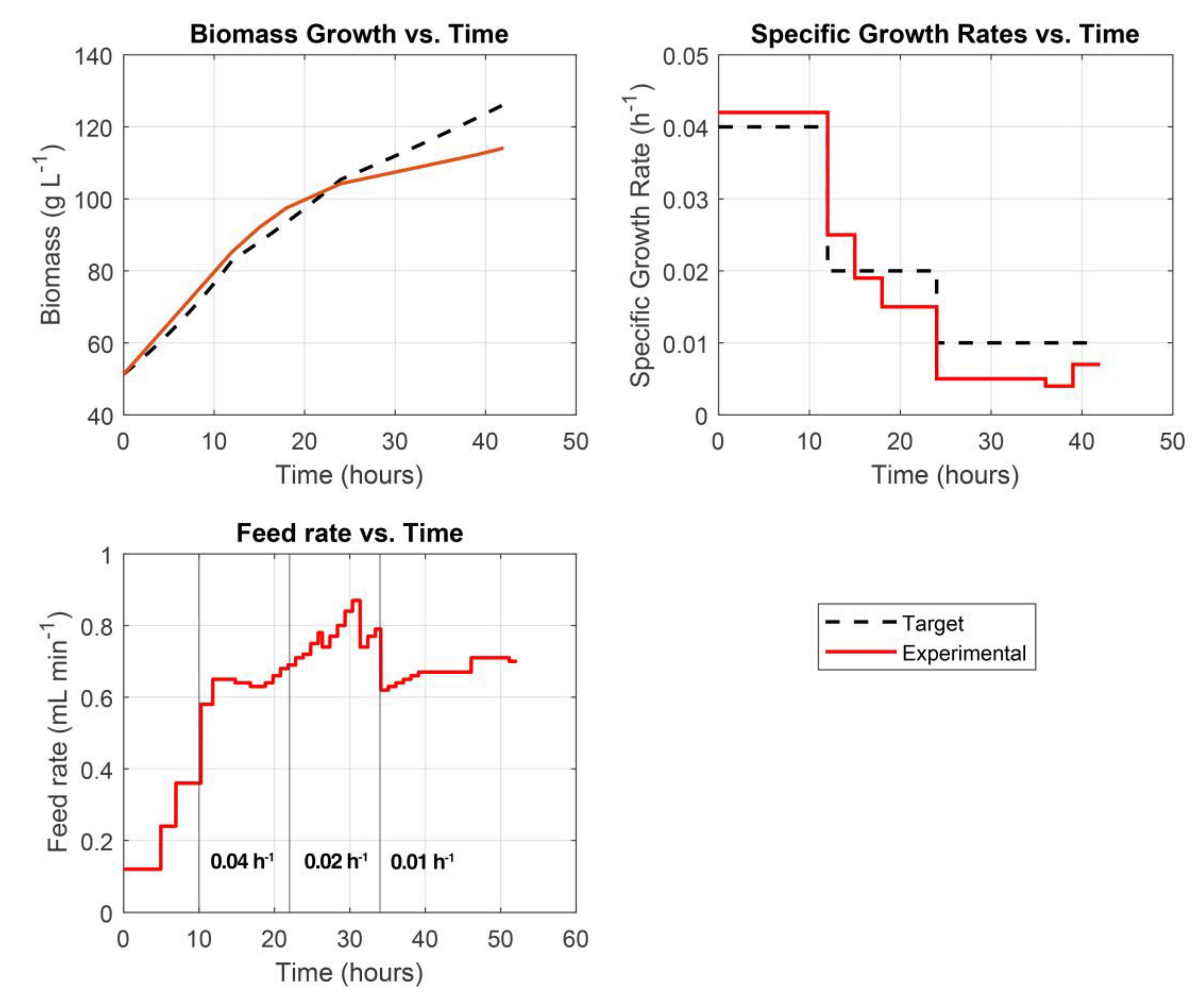

Table 1.
Dataset of P. pastoris fermentations and parameter ranges used for hybrid model training.
| Exp No. | Strain, product | Induction time, h | DCW, g·L-1 | Feed rate, mL·min-1 | Vend, L | Reference |
|---|---|---|---|---|---|---|
| 1* | GS115, HBcAg | 65 | 37.5—101.6 | 0.12—0.78 | 2.85 | [44,50] |
| 2* | GS115, HBcAg | 45 | 40.6—113.5 | 0.12—1.00 | 3.09 | |
| 3* | GS115, HBcAg | 43 | 41.2—120.1 | 0.12—0.98 | 3.13 | |
| 4* | GS115, HBcAg | 50 | 59.2—120.1 | 0.12—0.36 | 2.54 | |
| 5* | GS115, HBcAg | 51 | 41.4—96.6 | 0.12—0.36 | 2.87 | |
| 6 | GS115, HBcAg | 48 | 49.1—120.0 | 0.12—0.50 | 2.88 | |
| 7 | GS115, HBcAg | 43 | 53.7—101.5 | 0.12—0.36 | 2.74 | Unpublished data |
| 8 | GS115, CA IX | 54 | 44.1—84.0 | 0.12—0.56 | 2.75 | |
| 9* | X-33, LegH | 65 | 55.4—123.2 | 0.12—0.36 | 2.57 | [52] |
| 10* | X-33, LegH | 46 | 49.5—95.4 | 0.12—0.60 | 2.98 | |
| 11 | X-33, LegH | 65 | 48.9—111.2 | 0.12—0.36 | 2.85 | |
| 12 | X-33, LegH | 48 | 56.4—105.3 | 0.12—0.50 | 2.63 | |
| 13 | X-33, LegH | 50 | 45.3—101.3 | 0.12—0.36 | 2.61 | |
| 14 | X-33, LegH | 45 | 52.9—103.1 | 0.12—0.36 | 2.55 | |
| 15 | X-33, LegH | 46 | 45.1—101.3 | 0.12—0.36 | 2.52 | |
| 16 | X-33, LegH | 65 | 51.0—101.7 | 0.12—0.36 | 2.66 | |
| 17 | X-33, LegH | 46 | 50.6—92.4 | 0.12—0.60 | 3.00 | |
| 18 | X-33, Qβ | 65 | 52.5—117.6 | 0.12—0.49 | 3.23 | This research |
| 19 | X-33, Qβ | 48 | 49.3—117.2 | 0.12—1.00 | 3.40 | |
| 20 | X-33, Qβ | 55 | 50.1—107.7 | 0.12—0.36 | 2.84 |
*Experiments with real-time turbidity measurements.
Table 2.
Summary of the ten best-performing architectures from Bayesian optimization screening.
| First layer type | No. of FC layers | Hidden units | Nodes | Activation | Validation Loss (%) | No. of parameters | AICc |
|---|---|---|---|---|---|---|---|
| LSTM | 1 | 5 | 5 | Tanh | 9.73 | 268 | 2417 |
| 5 | 5 | LeakyReLu | 10.07 | 268 | 2431 | ||
| 5 | 4 | Tanh | 10.17 | 259 | 2312 | ||
| 1 | 5 | ReLu | 10.26 | 56 | 1126 | ||
| 5 | 5 | Tanh | 10.37 | 268 | 2444 | ||
| 3 | 5 | Tanh | 10.42 | 146 | 1448 | ||
| 4 | 5 | None | 10.51 | 203 | 1783 | ||
| 5 | 5 | Tanh | 10.68 | 268 | 2457 | ||
| 4 | 5 | ReLu | 10.75 | 203 | 1792 | ||
| 5 | 4 | Tanh | 11.30 | 259 | 2358 |
Table 3.
Summary of the best-performing architectures from grid search screening.
| Hidden units | Nodes | Activation | Validation Loss (%) | No. of parameters | AICc |
|---|---|---|---|---|---|
| 5 | 9 | LeakyReLu | 8.85 | 304 | 3050 |
| 4 | 10 | LeakyReLu | 9.27 | 243 | 2092 |
| 3 | 6 | LeakyReLu | 9.29 | 153 | 1427 |
| 3* | 5 | LeakyReLu | 9.37 | 146 | 1403 |
| 2* | 10 | LeakyReLu | 9.68 | 127 | 1334 |
| 2* | 9 | Tanh | 9.99 | 121 | 1316 |
| 2* | 8 | ReLu | 10.03 | 115 | 1302 |
| 1* | 9 | Tanh | 10.26 | 76 | 1189 |
| 1 | 6 | LeakyReLu | 10.21 | 61 | 1139 |
| 1 | 4 | ReLu | 10.25 | 51 | 1112 |
| 1 | 1 | Tanh | 10.36 | 36 | 1079 |
* Network architectures selected for the next optimization step.
Table 4.
Summary of the best-performing network architectures.
| Hidden units | Nodes | Activation | Validation Loss (%) | No. of parameters | AICc |
|---|---|---|---|---|---|
| 3 | 5 | LeakyReLu | 7.28 | 146 | 1294 |
| 2 | 10 | LeakyReLu | 6.37 | 127 | 1155 |
| 2 | 9 | Tanh | 8.14 | 121 | 1236 |
| 2 | 8 | ReLu | 4.93 | 115 | 998 |
| 1 | 9 | Tanh | 8.27 | 76 | 1090 |
Disclaimer/Publisher’s Note: The statements, opinions and data contained in all publications are solely those of the individual author(s) and contributor(s) and not of MDPI and/or the editor(s). MDPI and/or the editor(s) disclaim responsibility for any injury to people or property resulting from any ideas, methods, instructions or products referred to in the content. |
© 2025 by the authors. Licensee MDPI, Basel, Switzerland. This article is an open access article distributed under the terms and conditions of the Creative Commons Attribution (CC BY) license (http://creativecommons.org/licenses/by/4.0/).
Copyright: This open access article is published under a Creative Commons CC BY 4.0 license, which permit the free download, distribution, and reuse, provided that the author and preprint are cited in any reuse.


