Submitted:
03 July 2025
Posted:
07 July 2025
Read the latest preprint version here
Abstract
This paper proposes a novel theoretical model to explore the geometry of a closed universe, treating it as the crust of a four-dimensional sphere. Building upon the FLRW model and considering alternative cosmological scenarios, the study examines the motion of light in the fourth dimension to infer the universe's curvature. The approach involves mathematical modeling of spiral light trajectories, a theoretical framework for the nature of time across quantum and cosmic scales, and the determination of the universe's four-dimensional radius using Hubble's law. The model predicts the existence of mirror points and provides calculations of their positions relative to Earth under various parameters. This work aims to refine our understanding of the universe's structure and its implications for cosmology.
Keywords:
light propagation
; mirror points
; closed universe
1. Introduction
This paper presents a theory and then examines its results by calculating the path of light in the fourth dimension. According to the FLRW (Friedmann-Lemaître-Robertson-Walker) model, if the density of the universe exceeds the critical density , then the universe is geometrically closed [1,2,3]. The current calculated value for is approximately equal to one [4]. Certain cosmological models, such as those involving phantom energy, inhomogeneous cosmological models, additional matter formation, backreaction models, and future evolution of the universe, suggest that the current estimates of the universe’s density may be incorrect or subject to revision [5,6,7,8,9,10,11,12,13,14,15,16,17,18,19,20,21,22,23,24,25,26,27,28,29,30,31,32,33,34,35,36,37,38]. This could be important given possible future refinements in calculating the density of the universe. This paper attempts to consider a general model for the closed universe that is consistent with previously validated models describing cosmic phenomena such as general relativity, Hubble calculations and cosmological measurements [39,40,41].
A three-dimensional sphere has a two-dimensional surface (or crust). Similarly, a circle is two-dimensional, with its circumference being one-dimensional. In general, the boundary, or crust, of an object is one dimension lower than the object itself. Therefore, the crust of a four-dimensional sphere is a three-dimensional object. For two-dimensional beings living on the two-dimensional surface of a three-dimensional sphere, their universe appears flat and cannot be curved from their perspective. If the universe is closed, it appears flat to us. In this paper, the closed universe is modeled as the crust of a four-dimensional sphere, with the time axis aligned parallel to the sphere’s radius. This paper proposes an approach to understanding the universe’s curvature by analyzing the motion of light in the fourth dimension [43].
To investigate the motion of light in the fourth dimension, it is necessary to model the spiral motion based on physical quantities. Therefore, Section 2.1 is dedicated to mathematical modeling. In Section 2.2, a theory regarding the nature of time across quantum (small-scale) and cosmic (large-scale) dimensions is proposed, that demonstrates consistency with the physical phenomena described in Section 2.3. In Section 2.4, the radius of the universe’s four-dimensional sphere by applying Hubble’s law is determined. Moreover, the theory proposed in this model predicts the existence of mirror points in the universe. In the results section, based on different values for the parameters in the model, the positions of the mirror points and the farthest points in space relative to the Earth have been calculated.
2. The Model
2.1. Modeling Spiral Motion
In this section, we introduce a model for generating spiral motion in two dimensions. We assume that an object moves on a circle with a constant velocity B. Simultaneously, the radius of the circle increases over time at a constant rate V. To derive the equation of motion for this object, we first compute its angular velocity as follows:
where R(t) represents the radius of the circle as a function of time:
The angular displacement of the object can be obtained by integrating the angular velocity with respect to time, given by:
Utilizing Equations (2.2) and (2.3), we derive the parametric form of the object’s equations of motion as follows:
The polar equation for the golden spiral is as follows [42]:
where is the golden ratio. To facilitate a clearer comparison with equations (2.4) and (2.5), and to enable more effective plotting, we express equation (2.6) in its parametric form:
Now we present plots of the object’s equation of motion at a constant velocity V=1 across varying speeds of parameter B, compared to the golden spiral depicted in Figure 1, as follows:
Figure 1 demonstrates that when the ratio of the velocity of B to V is equal to , the resulting pattern closely approximates the Fibonacci golden spiral. Additionally, observing the diagrams from left to right in Figure 1, it is evident that increasing the velocity of B results in a greater curvature in the object’s motion. The key condition to demonstrate that an equation of motion describes a golden spiral is as follows [42]:
To verify condition (2.9) for Equations (2.4) and (2.5) at and , we select the arbitrary points as illustrated in Figure 2 (left). Also equation (2.9) was analyzed for the case where B and V are both equal to one. In this scenario (B=V), the result of the equation (2.9) is equal to 4.8. Consequently, for B=V=1, the equation of motion can be expressed in Figure 2 (right):
The Table 1 presents the specifications of the four selected points from Figure 2 (left), which are located along the object’s path, along with an review of Condition (2.9) as follows:
As shown in Table 1, the ratios obtained from the points are close to the value of . Therefore, in future calculations, we will employ Equations (2.4) and (2.5), using the velocity ratio for calculation on the Golden Spiral.
In the following section, we will explore the mechanisms of time at both the quantum (small-scale) and cosmic (large-scale) levels.
2.2. The Mechanism of Time
This section introduces a model for the nature of time. While the universe is typically described in three spatial dimensions, with time as the fourth perpendicular dimension, we simplify our discussion by considering space as one-dimensional for clarity.
According to Figure 3, consider two objects, A and B, moving through space. Object A moves at a slow velocity, while object B travels at the speed of light. Consequently, the smallest particles of object B cover a distance of one Planck length in each Planck time interval. In contrast, this is not the case for object A, whose particles move much more slowly.
As shown in Figure 3, in this model, the crusts in the fourth dimension that are parallel to each other. The smallest volume in the universe is a cube with a side length of one Planck length. A quantum model for the nature of time is proposed, where the information of each cube at a given Planck time is transferred to the next crust via an intermediate particle, which we have named Y. When an object moves faster, its movement in the fourth dimension becomes more inclined because the information of each cube associated with that object is transferred to the neighboring cube in the subsequent crust. The oblique motion of light in the fourth dimension results from its extremely high speed. Consequently, the angle formed during this motion corresponds to the angle within Einstein’s light cone. Since no particle can travel faster than the speed of light, information from a cube in one crust cannot be transmitted to more distant cubes in the next crust. This limitation can be exemplified by the restricted interaction of the intermediate particle Y, similar to the asymptotic freedom observed in gluons. Just as a gluon transfers color charge between quarks, a hypothetical Y particle could transfer information between two parallel crust. This information can be considered the smallest unit of energy, with the arrangement of these fundamental units giving rise to various basic structures. It is possible that an object’s high kinetic energy can trigger the activation of oblique movement of the intermediate particle Y. The size of particle Y in Figure 3 is hypothetical, and this particle functions as an intermediary between two parallel spaces, characterized by a metric distinct from that of conventional space.
If the density of the universe exceeds from the critical density, then the universe is closed. In this case, the three-dimensional space of the universe can be thought of as a crust of four-dimensional sphere. Because Figure 3 depicts a very small scale, this curvature is not readily apparent. However, in Figure 4, which illustrates the universe on a larger scale, the curvature of this space crust is visible as part of the encompassing four-dimensional sphere.
As illustrated in Figure 4, the light traveling from a galaxy to Earth follows the curved path marked in red, rather than the green path.
Therefore, the oblique motion of light in the fourth dimension at the quantum scale results in a corresponding oblique motion of light at the cosmic scale.
2.3. The Effects of Gravity on Spacetime
This section explores how gravity influences time. According to Figure 5, if we consider that the crust of three-dimensional space is curved along the time axis by placing a massive celestial body in space, then this crust expands towards the center of the four-dimensional sphere. This means that objects near this massive celestial body, are behind in time than other objects on this crust.
In Figure 5, we assume that a black hole is created in space at time (R) after the Big Bang (W) and disappears at time (P). In this case, the black hole bends spacetime around itself, which brings the crust closer to the center of the sphere. This causes time to run slower for objects near the black hole.
2.4. Evaluating Light Curvature
In this section, the motion of light on the surface of a growing four-dimensional sphere is evaluated based on the equations obtained from the Section 2.1. First, the current crust expansion rate is measured. So the arc length of a growing circle with radius and central angle is given by . Therefore, the crust growth rate is calculated as follows:
therefore, the farther an object is from Earth, the greater its escape velocity, since it subtends a larger central angle. So if we equate this relationship with Hubble’s relationship, we can calculate the radius of the four-dimensional sphere. If we assume that an asteroid is located one light year from Earth, its escape velocity from Earth for is given by the following equation:
Since the value of is equal to one light year, we obtain the radius of the four-dimensional sphere by equating equations (2.10) and (2.11), as follows:
The radius of the universe’s four-dimensional sphere for different parameter changes are calculated, as illustrated in the table below:
In Table 2, the values are in (). Also, the pertains to the golden spiral described in Section 2.1 and indicates the behavior of light traveling in the fourth dimension as modeled based on golden spiral. While the unit of R in Table 2 is the light year, it represents the axis of the fourth dimension, which, as shown in Figure 4, is perpendicular to space. Therefore, R effectively corresponds to a measure of time, with the unit of years. Therefore, the values in Table 2 represent the age of the universe corresponding to various parameter changes. The green cell in the Table 2 indicates the value closest to the measured age of the universe [41].
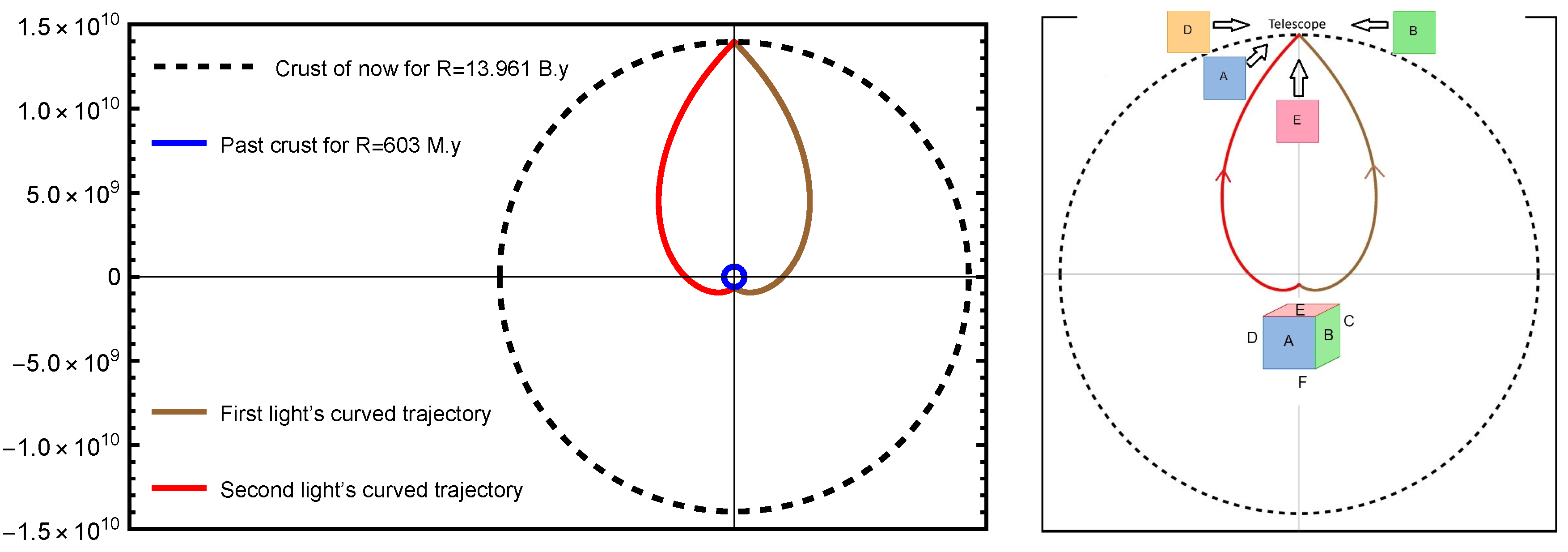
There are points in the four-dimensional space-time sphere of the universe that have two properties: first, they have a phase difference with respect to the Earth equal to integer multiples of , and second, if light emerges from the points of this spatial crust, it reaches Earth in current crust according to the path of the light spiral. To simplify notation, I have named these points "mirror points". For this reason, these points are named ’mirror points,’ because when a person stands between two mirrors, he can see both front and behind of himself simultaneously. In Figure 6, we depict the position of the first mirror point relative to Earth, based on calculations performed with Mathematica.
In Figure 6 (left), two light rays originating from a celestial body in the ancient crust (blue) are illustrated. The age of this crust is about 603 million years, determined from the universe’s age, which is indicated in green in Table 2. In fact, a powerful space telescope capable of zooming this far could capture images of the celestial object from two different perspectives: one from the front and another from the behind of the celestial object.
In Figure 6 (right), we have placed a hypothetical cube at a mirror point, on each face of this cube, the letters A, B, C, D, E and F are written. If a telescope in Earth’s orbit observes such a distance, depending on the telescope orientation position, it will see a different letter from this cube. In other words, by rotating the telescope around itself, it can see the image of the rotation of the cube.
Figure 6.
The position of the first mirror point relative to Earth within the four-dimensional sphere of the universe.
Figure 6.
The position of the first mirror point relative to Earth within the four-dimensional sphere of the universe.
Now we want to find the number of rotation of light within the four-dimensional sphere of the universe that it has traveled to reach us from one year after the Big Bang to the present.
In Figure 7, points C and E are mirror points, while point A has a phase difference of relative to point E. When zooming in graph, you’ll notice that the same shape is drawn inward from E point, creating a repeating pattern to inner. Using the plotting tool in Mathematica, The R ratios were calculated for the points in the Figure 7 until the approached 1. The corresponding values of these ratios are determined as follows:
The number of cycles observed with the drawing tool in Mathematica ranged from 3 to 4 cycles. However, to precisely determine its value, we apply Equation (2.13) as follows:
If we consider to represent one year after the Big Bang, then the number of cycles for become =(3.722). Since the number of mirror points is twice the number of rotations (excluding point A itself), the total number of mirror points at these parameter values is 7.
In the following section, we determine the number of mirror points and their respective locations for various parameter values within the model.
3. Results
In the previous section, we did not analyze the model for values of R less than one year, because, in the early stages of the universe, light had enough time to traverse the crust of entire four-dimensional sphere of the cosmos within just a few years. This greatly increased the likelihood of photons colliding with matter, making it improbable for us to observing the universe’s earliest moments. According to this model, the early universe remains invisible to our eyes appearing dark and yet is exceedingly luminous from itself perspective. The age of the mirror points by year () are calculated based on different values of the universe age, which are given in Table 2 and the calculations in Section 2.3, as follows:
For Table 3, we selected only those values of the universe age from Table 2, that are not inconsistent with cosmological observations and less than 13 billion years. As can be seen in Table 3, the density of mirror points is higher in the early times. And light has performed most of its cycles in the beginning of the universe.
Since if we move in a closed universe in one arbitrary direction at a speed in a straight line, after a
while we will return to our original position from the opposite direction, therefore the point on the
current crust that is farthest from Earth () in 3D space, lies beyond the four-dimensional sphere, and its distance from Earth is . This means that if an object moves in a straight line through space at a constant speed, it will approach the Earth when it passes this point (). This means that space is closed. The volume of the current crust of four-dimensional sphere () can be obtained from the formula . But, the volume of a four-dimensional sphere () is obtained from the formula , which represents the total volume of the universe’s spacetime [43].

Table 4.
The values of (), () and () for results of in Table 2.
Table 4.
The values of (), () and () for results of in Table 2.
4. Conclusion
In this paper, a suitable physical modeling was obtained for the golden spiral and the movement of light at (B=V). The presented model aligns well with Einstein’s light cone concept and accurately reflects the influence of gravity on spacetime within the framework of general relativity. The presented model effectively bridges the concept of time at both the quantum (small-scale) and cosmic (large-scale) levels. Since hypothetical particles Y are exchanged between two parallel universes, they can be interpreted as a new force that holds the two planes of the universe together. According to the values obtained from Table 2, it can be concluded that the idea of light moving in the fourth dimension according to the golden spiral is not correct. Rather, light moves in the fourth dimension at (B=V). This conclusion is reinforced by the correlation between the values in Table 2 and the observed measurements of the universe’s age. The mechanism of expansion of the space-time crust in this model is in good agreement with the Hubble’s law. The model presented in this paper predicts mirror points,
which will make this model verifiable. The verification of this model involves observing that when
a powerful telescope looks at celestial body located at mirror points positions relative to Earth, the
images of celestial body will rotate accordingly as the telescope rotates around its own axis.
Data Availability Statement
The Mathematica files and data supporting the results are available at here.
References
- A. Friedman, Z. Phys. 10 (1922), 377-386. [CrossRef]
- G. Lemaitre, Nature 127 (1931), 706. [CrossRef]
- P. J. E. Peebles, Princeton University Press, 2020, ISBN 978-0-691-20981-4.
- N. Aghanim et al. [Planck], Astron. Astrophys. 641 (2020), A6 [erratum: Astron. Astrophys. 652 (2021), C4]. [CrossRef]
- S. Nojiri and S. D. Odintsov, Phys. Rept. 505 (2011), 59-144. [CrossRef]
- T. Buchert, Gen. Rel. Grav. 32 (2000), 105-125. [CrossRef]
- D. Harlow, M. Usatyuk and Y. Zhao, [arXiv:2501.02359 [hep-th]].
- A. G. Suvorov, Phys. Rev. D 111 (2025) no.2, 023508. [CrossRef]
- M. Kamionkowski and N. Toumbas, Phys. Rev. Lett. 77 (1996), 587-590. [CrossRef]
- K. Bamba, S. Capozziello, S. Nojiri and S. D. Odintsov, Astrophys. Space Sci. 342 (2012), 155-228. [CrossRef]
- M. N. Celerier, Astron. Astrophys. 353 (2000), 63-71 [arXiv:astro-ph/9907206 [astro-ph]].
- A. D. Linde, [arXiv:hep-th/0211048 [hep-th]].
- H. Alnes, M. Amarzguioui and O. Gron, Phys. Rev. D 73 (2006), 083519. [CrossRef]
- K. Bolejko, M. N. Celerier and A. Krasinski, Class. Quant. Grav. 28 (2011), 164002. [CrossRef]
- S. Rasanen, JCAP 11 (2006), 003. [CrossRef]
- S. Cespedes, S. P. de Alwis, F. Muia and F. Quevedo, Phys. Rev. D 104 (2021) no.2, 026013. [CrossRef]
- B. Ratra, Phys. Rev. D 96 (2017) no.10, 103534. [CrossRef]
- C. R. Nappi and E. Witten, Phys. Lett. B 293 (1992), 309-314. [CrossRef]
- C. Clarkson, G. Ellis, J. Larena and O. Umeh, Rept. Prog. Phys. 74 (2011), 112901. [CrossRef]
- A. H. Guth and P. J. Steinhardt, Spektrum Wiss. 7 (1984), 80-94.
- M. P. Dabrowski, T. Stachowiak and M. Szydlowski, Phys. Rev. D 68 (2003), 103519. [CrossRef]
- S. Dutta and I. Maor, Phys. Rev. D 75 (2007), 063507. [CrossRef]
- S. Weinberg, John Wiley and Sons, 1972, ISBN 978-0-471-92567-5, 978-0-471-92567-5.
- R. R. Caldwell, M. Kamionkowski and N. N. Weinberg, Phys. Rev. Lett. 91 (2003), 071301. [CrossRef]
- E. W. Kolb and M. S. Turner, Front. Phys. 69 (1990), 1-547 Taylor and Francis, 2019, ISBN 978-0-429-49286-0, 978-0-201-62674-2. [CrossRef]
- L. H. Ford, Phys. Rev. D 14 (1976), 3304-3313. [CrossRef]
- G. F. R. Ellis, P. McEwan, W. R. Stoeger, S.J. and P. Dunsby, Gen. Rel. Grav. 34 (2002), 1461-1481. [CrossRef]
- M. Vogelsberger, S. Genel, V. Springel, P. Torrey, D. Sijacki, D. Xu, G. F. Snyder, D. Nelson and L. Hernquist, Mon. Not. Roy. Astron. Soc. 444 (2014) no.2, 1518-1547. [CrossRef]
- S. Nojiri and S. D. Odintsov, eConf C0602061 (2006), 06. [CrossRef]
- W. Handley, Phys. Rev. D 103 (2021) no.4, L041301. [CrossRef]
- S. Gratton, A. Lewis and N. Turok, Phys. Rev. D 65 (2002), 043513. [CrossRef]
- S. Kalyana Rama, Phys. Lett. B 457 (1999), 268-274. [CrossRef]
- D. Burgarth and P. Facchi, [arXiv:2506.03254 [quant-ph]].
- M. Sami and A. Toporensky, Mod. Phys. Lett. A 19 (2004), 1509. [CrossRef]
- J. Lesgourgues and T. Tram, JCAP 09 (2014), 032. [CrossRef]
- J. M. Cline, S. Jeon and G. D. Moore, Phys. Rev. D 70 (2004), 043543. 2004. [CrossRef]
- B. J. Carr, K. Kohri, Y. Sendouda and J. Yokoyama, Phys. Rev. D 81 (2010), 104019. [CrossRef]
- V. B. Bezerra, G. L. Klimchitskaya, V. M. Mostepanenko and C. Romero, Phys. Rev. D 83 (2011), 104042. [CrossRef]
- A. Einstein, Annalen Phys. 49 (1916) no.7, 769-822. [CrossRef]
- E. Hubble, Proc. Nat. Acad. Sci. 15 (1929), 168-173. [CrossRef]
- D. N. Spergel et al. [WMAP], Astrophys. J. Suppl. 148 (2003), 175-194. [CrossRef]
- J. R. Chasnov, Int. J. Math. Sci. 10 (2016), 123-145.
- G. B. Arfken, H. J.Weber, F. E. Harris, Academic Press, 7th edition, 2011.
Figure 1.
Plotting the spiral motion of an object with varying speeds B and V=1, in comparison to the golden spiral.
Figure 1.
Plotting the spiral motion of an object with varying speeds B and V=1, in comparison to the golden spiral.

Figure 2.
Comparison of the Golden Spiral with its physically modeled alternative (left), and of motion with constant velocity parameters versus its modeled counterpart (right).
Figure 2.
Comparison of the Golden Spiral with its physically modeled alternative (left), and of motion with constant velocity parameters versus its modeled counterpart (right).
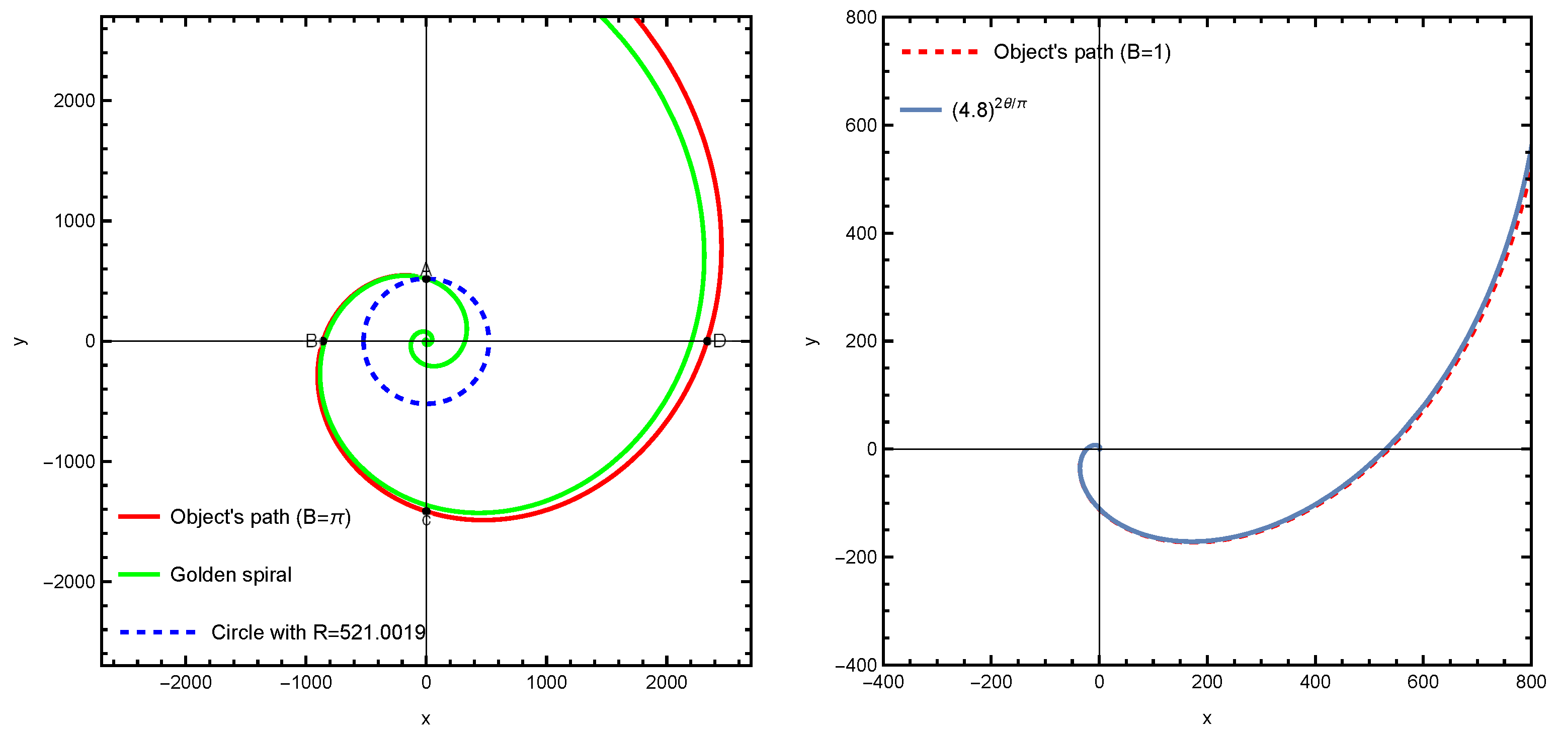
Figure 3.
Illustration of the time mechanism for the space crust at the quantum scale and its comparison with Einstein’s light cone.
Figure 3.
Illustration of the time mechanism for the space crust at the quantum scale and its comparison with Einstein’s light cone.
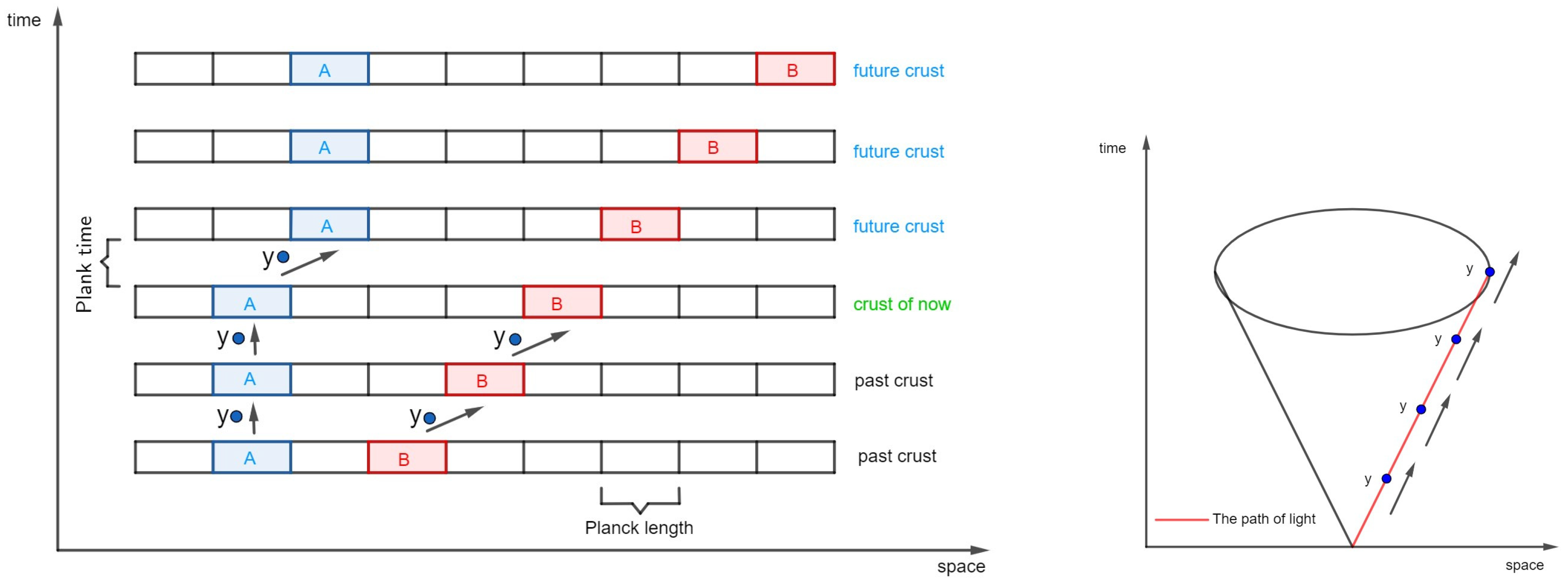
Figure 4.
The curvature of the light path from a distant galaxy within the four-dimensional sphere of the universe as it reaches Earth.
Figure 4.
The curvature of the light path from a distant galaxy within the four-dimensional sphere of the universe as it reaches Earth.
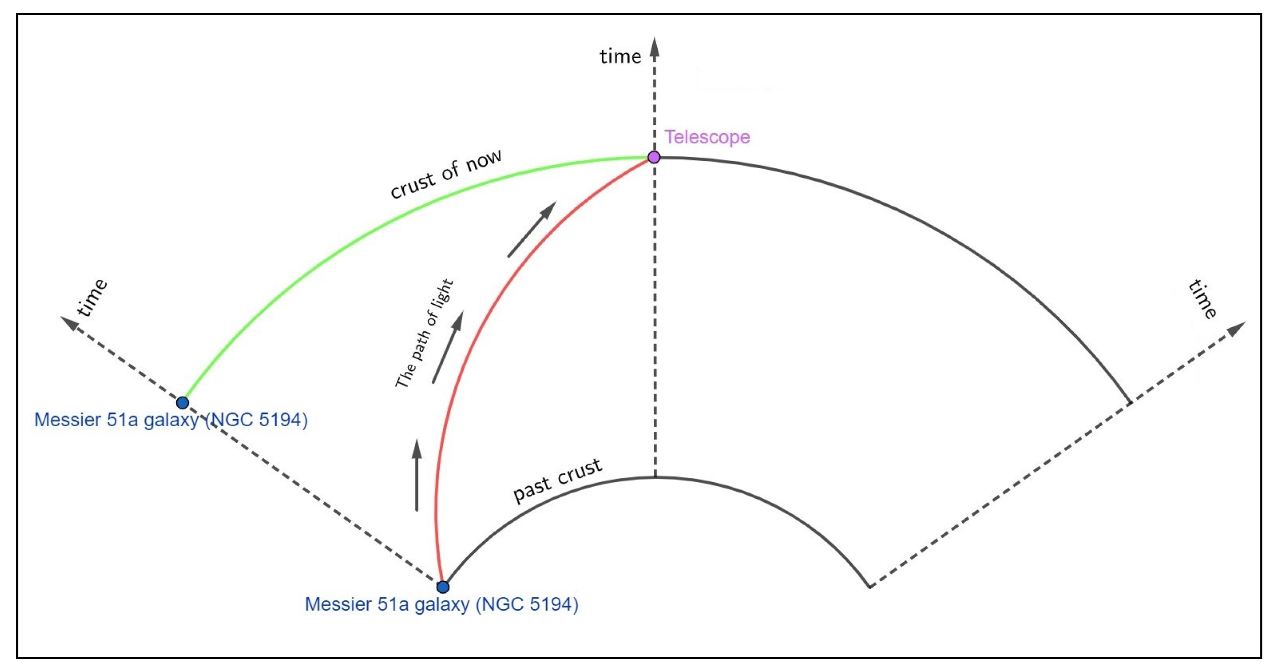
Figure 5.
The curvature of the space crust throughout the birth (R point) and death (P point) phases of a black hole within the four-dimensional sphere of the universe.
Figure 5.
The curvature of the space crust throughout the birth (R point) and death (P point) phases of a black hole within the four-dimensional sphere of the universe.
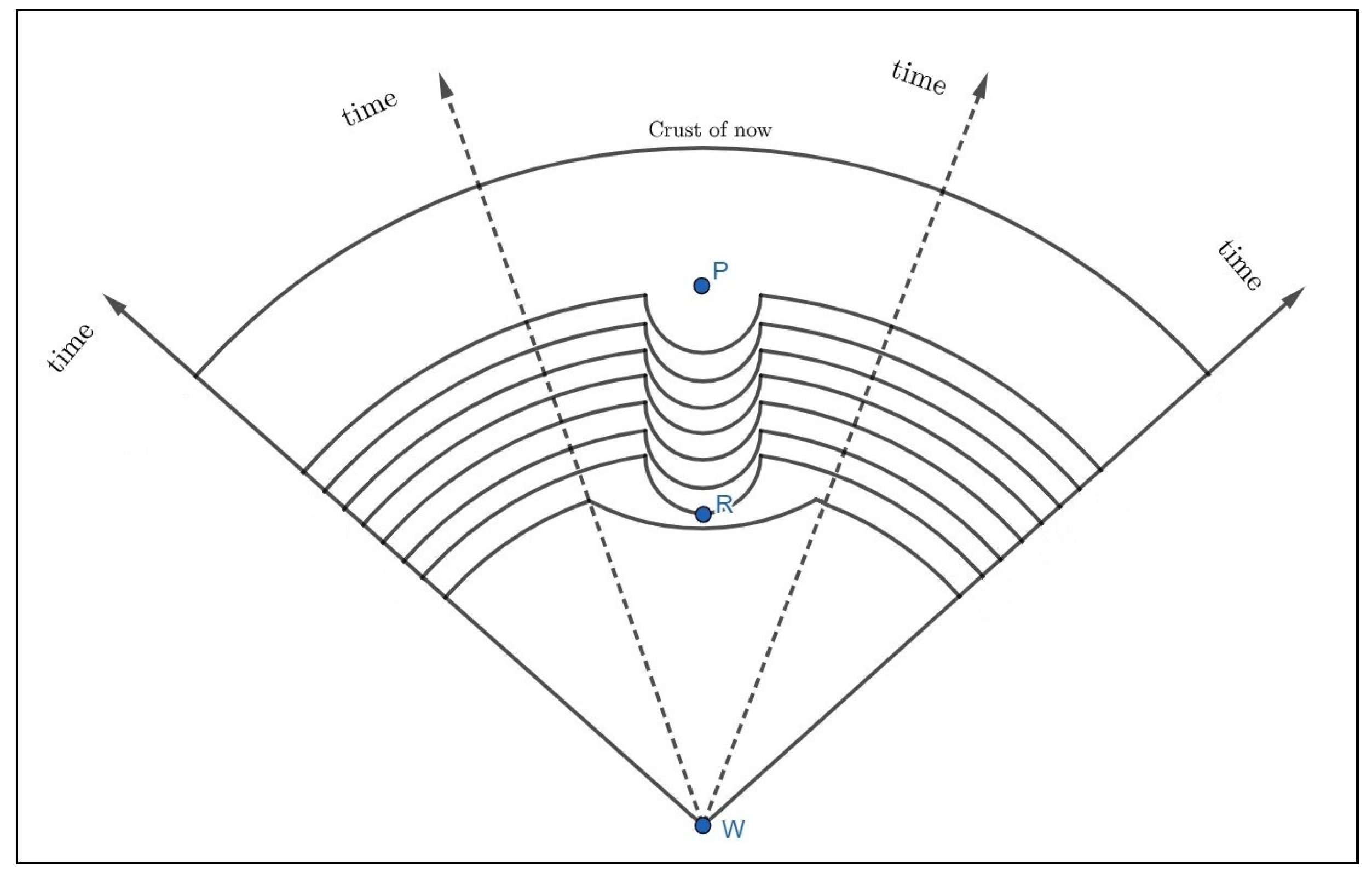
Figure 7.
The positions of four points, each with a phase difference of , during the final complete cycle of light reaching Earth within the four-dimensional sphere of the universe.
Figure 7.
The positions of four points, each with a phase difference of , during the final complete cycle of light reaching Earth within the four-dimensional sphere of the universe.
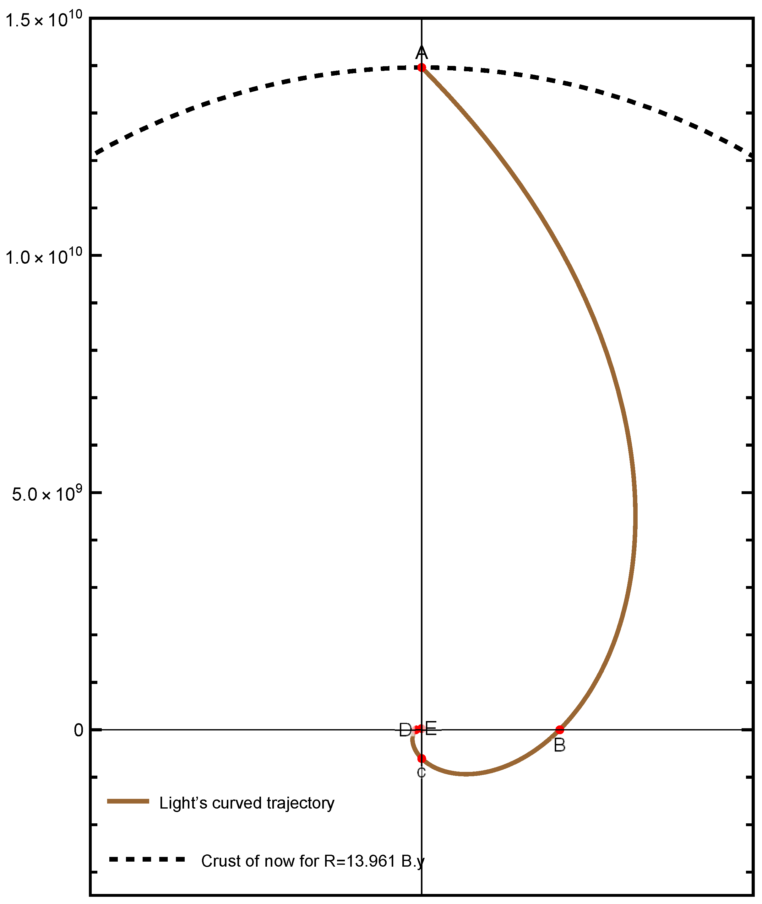
| Points | ||
| A | 521 | 1.648 |
| B | 859 | 1.650 |
| C | 1418 | 1.643 |
| D | 2330 | - |
Table 2.
Variation of the Universe’s Radius Corresponding to Different Hubble Constant Values.
Table 3.
The time of mirror points after the Big Bang for results of in Table 2.
Table 3.
The time of mirror points after the Big Bang for results of in Table 2.
Disclaimer/Publisher’s Note: The statements, opinions and data contained in all publications are solely those of the individual author(s) and contributor(s) and not of MDPI and/or the editor(s). MDPI and/or the editor(s) disclaim responsibility for any injury to people or property resulting from any ideas, methods, instructions or products referred to in the content. |
© 2025 by the authors. Licensee MDPI, Basel, Switzerland. This article is an open access article distributed under the terms and conditions of the Creative Commons Attribution (CC BY) license (http://creativecommons.org/licenses/by/4.0/).
Copyright: This open access article is published under a Creative Commons CC BY 4.0 license, which permit the free download, distribution, and reuse, provided that the author and preprint are cited in any reuse.


