
Submitted:
03 July 2025
Posted:
04 July 2025
You are already at the latest version
Abstract
The use of renewable energy sources (RESs) in modern electric grids poses considerable challenges regarding the balance of supply and demand and the cost-effective operation of the grid. In this paper we present the decentralized energy management system (EMS) to reduce operational costs, to cope with uncertainties of the renewable generation and load demand. The solution involves employing a machine-learning-based approach, the multilayer perceptron artificial neural network (MLP-ANN), to develop precise forecasts of photovoltaic and wind turbine generation, ambient temperature, and load demand. Of the two tested training algorithms (Levenberg-Marquardt (LM) and resilient backpropagation (RP), LM had the best predictive performance. The newly proposed Modified Cheetah Optimizer (MCO) algorithm eliminates the common local trapping and premature convergence issue possessed by the traditional optimization methods to optimize generation scheduling. The integrated EMS based on MCO achieves an impressive reduction of 26.8% in operational cost in comparison with traditional methods. In addition, the adoption of a DR program leads to a peak load decrease by 7.5% and a valley load filling increase by 9.6%. Through simulation results, we find that the proposed framework improves the forecast accuracy up to 15%, resulting in a more resilient and economic microgrid management strategy. The impacts of matching machine learning forecasting with enhanced optimization methods and solving methodologies may turn into a breakthrough in microgrid operational optimizations and economic advantages, as the work emphasizes.
Keywords:
decentralized energy management system
; machine learning
; forecasting
; renewable energy sources
; microgrid optimization
; demand response
; operational cost reduction
; uncertainty management
; photovoltaic generation
; wind turbine generation
1. Introduction
Recently, there has been global attention to renewable energy sources due to increased issues about climate change and depleting reserves of fossil fuel [1]. Microgrids have turned out to be a suitable solution in integrating renewable energy sources (RESs) while maintaining grid stability. Microgrids develop evolutionary flexibility in participation in diversified energy resources, moving energy generation closer to consumption points and reducing transmission losses. The operational complexities imposed on the variability by the load demand, as well as those because of photovoltaic (PV) and wind turbine (WT) generations, inherently call for advanced techniques when it comes to forecasting and optimization.
The need for renewable energy sources—efficient microgrid development, accurate forecasting of renewable power generation, and active load demand performance—plays a large role in conducting an efficient procedure in microgrid operations. Traditional procedures using time series analysis [2], and several statistical techniques hold low accuracy related to the stochastic and nonlinear operative natures in RESs [3], whereas conventional procedures of optimization with higher nonlinear and extensive dimensional constraints fail to obtain a globally optimal solution that characterizes planning or scheduling of microgrids [4]. These limitations point to the need for novel approaches in data-driven forecasting and optimization for better performance of energy management systems (EMSs).
Precise forecasting of renewable generation is one of the key challenges in energy management within microgrids. Due to the stochastic and intermittent nature of PV systems and WTs, complexity in power generation scheduling has increased a lot and requires advanced predictive models. Traditional methods, such as statistical and deterministic approaches, normally cannot predict the nonlinear nature of renewable sources. This deficiency may lead to suboptimal energy management, lower system reliability, and higher operational costs [5]. Recent advances in machine learning (ML) techniques have opened new avenues for surmounting the challenges found in forecasting. These techniques, especially artificial neural networks (ANN), have been more successful than the old techniques in dealing with the main difficulties of complex nonlinear relationships that are usually present in energy forecasting. As such, multilayer perceptron ANNs (MLP-ANN) have been applied quite successfully in the estimation of PV and WT output using past data and meteorological variables, while out of the several training algorithms, Levenberg-Marquardt (LM) stands superior as compared to others such as resilient backpropagation (RP) for its high degree of accuracy and swiftness of convergence [6,7,8].
The more sophisticated models, such as Support Vector Regression (SVR), have also shown a lot of promise. For instance, Singh et al. [9] discussed how SVR models that were trained on extensive datasets, including historical energy production and meteorological conditions, were able to make improvements in forecasting accuracy and hence permit better resource allocation with reduced operational costs.
Other works also confirm the efficiency of machine learning models in renewable energy forecasting. Grève et al. [10], for instance, propose a hybrid ensemble model. The work combined two neural network algorithms, bidirectional long short-term memory with mixed integer linear programming, and two tree-based techniques, namely gradient boosting decision tree and random forest (RF), to improve local wind power generation forecasting. This ensemble model outperformed the performance of individual algorithms, improving the Root Mean Squared Error (RMSE) by 10% and hence providing a more reliable forecast for day-ahead predictions. In the work of Dimitropoulos et al. [11], it was proposed, for the short-term prediction of energy generation in a community solar plant other machine learning algorithms like extreme gradient boosting, SVR, and long short-term memory. Out of these, there resulted in great reductions of RMSE, ensuring that the outperforming was done by the XGBoost model at all the considered models. These results further confirm that ML can predict energy production with a high degree of accuracy, a critical factor in the optimization of energy supply and distribution in microgrids.
Besides, some recent works have targeted the inclusion of ensemble learning and advanced ML algorithms to enhance forecasting accuracy. Wu et al. [12] developed flexible multi-time-period fuzzy uncertain demand response models for optimizing load forecasting with the aim of network stabilization, hence further enhancing robust energy management systems. Other techniques that have been successful in overcoming the limitations of single models include ensemble methods, such as Gradient Boosting Regression (GBR), RF, and hybrid frameworks within the scope of both forecasting and load management. The combined wavelet transformations and ML models show great potential in handling nonlinear periodic patterns of renewable energy data sets for more accurate predictions and better energy management performance [13].
In the context of optimization, particle swarm optimization (PSO) and genetic algorithm (GA) have been two of the popular metaheuristic algorithms long used in scheduling within microgrids due to their ability to handle complex constraints [2,14]. However, methods using these algorithms have generally been criticized for several reasons, including premature convergence and computational inefficiency when applied in high-dimensional space, hence restricting their applicability in more complex microgrid settings. Some researchers have tried to overcome such defects by using enhanced PSO methods, like second-order oscillatory chaotic mapping PSO and velocity differential evolutionary PSO, aiming at improving both the computational efficiency and the robustness of such energy management under uncertainty [15,16]. These approaches have fared well in improving the performance of energy systems under dynamic and uncertain operational conditions.
In this direction, several hybrid optimization approaches have recently appeared that combine PSO with the most advanced techniques, such as primal-dual interior point methods and multi-agent system-based frameworks [17,18]. Such hybrid models aim at providing even better performances in microgrid operation by properly exploiting the flexibility of PSO and the accuracy of more deterministic methods. It is such hybridization that has been able to address the concerns of system efficiency, power quality, and fuel consumption—issues that are of prime importance for real-world optimization of microgrid operation.
Besides, several recently proposed advanced strategies to mitigate issues related to energy management within microgrids. Within this context, the two-layer energy management system in [19] efficiently performed the optimization process of matching between batteries and fuel costs, with the help of goal programming techniques, proving that by increasing battery lifetimes, there would be a chance to reduce the total operating costs. Other metaheuristics, such as memory-based genetic algorithms [20] and grey wolf optimization [21], have also been applied with considerable success to optimize power distribution, reduce costs, and handle renewable variability. Advanced particle swarm optimization methods [22] have also shown potential in providing 24-hour forecasts for load and renewable energy variations, thus ensuring better system adaptability.
Hybrid approaches have also significantly enhanced energy management strategies. Fuzzy logic hybridized with grey wolf optimization has efficiently implemented operational cost minimization and fossil fuel emissions by optimally utilizing batteries and minimizing the dependency on conventional energy [23]. Chaotic and fuzzy self-adaptive particle swarm algorithms have also shown their effectiveness in the microgrid to minimize emissions and reduce costs in multi-objective optimization challenges [24]. Stand-alone microgrids have already adopted optimization techniques such as the application of a genetic algorithm in the optimal placement of renewable resources and storage devices. Such optimization techniques, by considering environmental variables such as wind and solar irradiance, optimized lifecycle costs while assuring efficient energy use [25].
Put together, these developments point to a rising role in advanced metaheuristics and hybrid optimization methods in solving the complexities of microgrid operation. These methods address issues such as computational inefficiency, resource variability, and system adaptability, thus paving the way for more sustainable and cost-effective energy management solutions in dynamic and uncertain operational contexts.
With an increasingly important emphasis on integrating multiple energy sources and optimally managing the energy, more advanced developments in control strategy are driven. For example, Abd-Elhaleem et al. developed an intelligent power management system for PHEV using a chaotic enhanced generalized particle swarm optimization-based interval type-2 Takagi-Sugeno-Kang fuzzy controller [26]. Their methodology presented evidence of energy savings concerning the conventional methods, but it also has a big disadvantage: the fact that the system proposed was only simulated and not tested in real conditions. On the other hand, Aguila-Leon et al. [27] proposed an auto-tunable energy management system for microgrids based on ANN optimal with PSO. This system showed remarkable improvements in forecast accuracy, although, with its high reliance on computational resources, practical feasibility concerns are raised with respect to real-time applications.
Going further with the optimization techniques, Ferahtia et al. proposed an SSA-based energy management strategy for a DC microgrid that contains various power sources, such as renewables, fuel cells, and battery storage [28]. Their model showed better performance in terms of fuel savings and power quality compared to conventional PSO-based systems; however, the authors mentioned that more tests should be conducted in different real-world scenarios to be able to fully assess the robustness of the system.
Besides, demand-side management strategies, as analyzed by Thornburg et al. [29], have already turned out to be viable in the context of an isolated system with high renewable energy penetration. These are demand-shifting, and peak-shaving applied to specific scenarios characterized by variability and uncertainty of renewable generation that give a great contribution to enhancing the reliability and efficiency of the systems.
While significant progress has been made in forecasting and optimization for microgrid EMSs, several gaps remain. For instance, most of the existing forecasting models are far from fully capturing the complex nonlinear interactions among photovoltaic generation, wind turbine output, ambient temperature, and load demand, which significantly limits their accuracy under variable and dynamic conditions. While ANN-based models, especially MLP ANNs, have been very successful in forecasting PV and WT outputs using historical data and meteorological variables [6,7], their use within a general framework of energy management systems has not been sufficiently investigated. Most previous work has concentrated on enhancing the accuracy of the forecasts without considering how these models could be integrated within a general framework of energy optimization and decision-making. Besides, the LM training algorithm has been proved to be more accurate and with higher convergence speed compared to some other methods, such as resilient backpropagation, but its power for solving dynamic and uncertain microgrid environment problems is yet to be tapped. Development and implementation of an MLP-ANN-based forecasting model within energy management systems could bridge the gap in allowing better accuracy and more informed decision-making.
Besides, most conventional optimization techniques also lack the potential to balance exploration and exploitation effectively, hence resulting in suboptimal scheduling solutions when dealing with high-dimensional nonlinear constraints. This drawback is further exacerbated by the fact that most of the approaches ignore the correlations among the forecasted variables, hence leading to a lot of inefficiencies in scheduling and resource allocation. These challenges call for novel approaches that will integrate advanced forecasting techniques with robust optimization frameworks to enhance the overall efficiency and performance of EMSs.
To address these gaps, this paper proposes an advanced EMS for microgrids that will incorporate sophisticated forecasting and optimization techniques. The major contributions of this research work are as follows:
- Development of ML-based forecasting models using MLP-ANN trained with LM and RP algorithms for the prediction of PV and WT generation, ambient temperature, and load demand. The proposed approach will have higher accuracy; LM performed better as compared to RP.
- In this paper, the MCO algorithm is proposed, adding advanced mechanisms of exploration and exploitation to traditional metaheuristic approaches, like cheetah optimizer (CO) [30], PSO, and teaching–learning-based optimization (TLBO) [31] algorithms. MCO successfully solves microgrid scheduling problems containing high-dimensional and nonlinear optimization.
- Incorporation of the DR program within the EMS to handle peak and valley loads will help to ensure that the balance between the supply and consumption of electricity will be much better. This reduces operation costs.
- A consideration of correlations among forecasted variables to enhance the reliability and adaptability of the EMS in its operating modes under uncertainty.
The proposed EMS provides a robust solution for cost-effective and reliable microgrid operation by combining high accuracy forecasting with a well-advanced optimization framework, thus contributing to the broader adoption of renewable energy technologies.
The rest of the paper is organized as follows: Section 2 defines the optimal EMS’s formulation; Section 3 presents the proposed MLP-ANN forecasting method. Section 4 presents the proposed MCO algorithm in detail. Section 5 discusses the simulation results regarding system performance. Finally, Section 6 concludes this paper and advises on further areas of research.
2. Problem Formulation
The optimization problem for the EMS is defined in this section, with an emphasis on optimal generation scheduling. The primary goal is to reduce operational costs, which are subject to a variety of constraints, including power balance constraints, spinning reserves constraints, generation capacity constraints, and DR constraints.
2.1. Objective Function
The optimization goal is to achieve a compromise between the reduced total operational cost of the generation units deployed at the generation locations and the costs associated with a specific DR. The objective function can be constructed in the following manner:
where the system’s total operational cost is denoted as . indicates the operational expenses of renewable generation (WT and PV with the cost coefficients of and , respectively) at their respective nodes. represents the cost of purchasing power from the primary utility, which is susceptible to time-of-use (TOU) pricing (). The cost associated with diesel generators, including their operational costs, is denoted by , which is calculated using specific cost coefficients and for diesel generator i. The costs associated with the demand response program are denoted by and are elaborated upon below.
2.2. Demand Response Program
DR comprises the demand resources designed and implemented to provide specific demand reduction and to enhance grid stability through voluntary load reduction. Costs for the demand response program are defined as follows:
where:
• denotes the voluntary load reduction in the DR program at time .
• illustrates the cost coefficient of interruptible/curtailable (I/C) loads.
The load reduction is constrained by:
where:
• represents the power demand at time .
• It is assumed that only 20% of the total demands participate in the load response program.
2.3. System Constraints
To guarantee the solution’s reliability and feasibility, the subsequent constraints must be considered:
2.3.1. Power Balance Constraint
The balance constraint of power guarantees the sum of all generated power at every millisecond is equal to the demand at that moment. Mathematically, this is depicted by:
where:
• represents the total power demand at time .
• is the total number of wind units, and is the total number of PV units.
This restriction guarantees that the energy generated by all sources matches the energy demanded by consumers to maintain grid stability.
2.3.2. Spinning Reserves Constraint
The constraint of spinning reserves becomes important to deal with unexpected power outages and sudden changes in load. This can be expressed as:
where:
• represents the total generation capacity of the system at time .
• denotes the line losses during the transmission of power.
Therefore, the system is rendered more reliable by guaranteeing that generation capacity will consistently satisfy demand and mitigate potential losses.
2.3.3. Generation Capacity Constraints
It is imperative that the generation of each generating unit is within the designated parameters. The capacities of PV, wind, and diesel generators deployed at their respective nodes are limited by the following:
where: and are the minimum and maximum generation capacities for the PV units, respectively. Similarly /, /, and / define the minimum/maximum capacities for wind turbines, each type of diesel generator, and the grid, respectively.
2.4. Problem Solution (Decision Variables) Representation
These are the optimization problem’s decision variables, and they reflect power generating outputs from all energy sources as well as demand response at each time step. To address the optimization issue, the MCO method combines all these decision variables into a single vector.
The decision vector X is organized as follows:
The total length of the decision vector X is given by:
where:
• : Number of time steps in the optimization horizon.
• : Number of photovoltaic (PV) units.
• : Number of wind turbines.
• : Number of diesel generators.
• The represents the power purchased from the grid and the demand response for each time step .
As a result, the decision vector X provides a compact representation for all energy sources’ power generation scheduling and demand response, which will be optimized by the proposed MCO method.
3. Machine Learning Forecasting Approach
3.1. Data Collection and Processing
The development process for the proposed model, specifically MLP-ANN, begins with the collection and processing of data. Therefore, the dataset includes temporal, meteorological, and environmental variables that are pertinent for predicting solar irradiance, ambient temperature, wind speed, and energy demand. The primary characteristics include the time of day, the day of the week, humidity levels, and the percentage of cloud cover.
Normalization techniques were applied to scale the data within the range of to 1, enhancing numerical stability and accelerating convergence. The mathematical representation of min-max scaling is expressed through the following formula:
where and . The processed dataset was divided into 70% for training, 15% for validation, and 15% for testing.
The proposed structure is designed on three significant layers for the MLP model: an input layer, a hidden layer, and an output layer. The model can also contain one or more activation functions in the hidden layer. To determine the best predictive model for solar irradiance, ambient temperature, wind speed, and energy demand, this study employs two training methods, namely LM and RP. This network features two hidden layers, designated as H1 and H2, which comprise 2 neurons in the first layer and 3 neurons in the second layer. Following several attempts and evaluating various alternatives, the log-sigmoid activation function [32] was selected for the first hidden layer, while the SoftMax [33] was designated for the second layer. The output layer employed a linear activation function. Figure 1 and Figure 2 illustrate the configuration of MLP-ANN and the overarching architecture of the neural network, respectively. Figure 1 demonstrates the methodology employed for training and testing utilizing MLP-ANN to predict four distinct outputs. Figure 2 illustrates the transfer functions integrated within the model.
3.2. Principles of MLP-ANN
The MLP-ANN was structured with a single input layer that aligns with the specified inputs, complemented by two hidden layers and a single output layer, engineered to simultaneously predict all four target variables. The output of the MLP-ANN can be expressed as follows:
where:
• is the input feature vector,
• and are activation functions for the hidden and output layers, respectively,
• are the weight matrices for the hidden and output layers,
• are the bias vectors.
The architecture comprises two hidden layers, featuring 2 neurons in the initial layer H1 and 3 neurons in the subsequent layer H2. Within this configuration, the activation function for the first hidden layer, denoted as , is characterized by a logarithmic sigmoid function defined as:
The model becomes non-linear because of this. Since the SoftMax activation function is capable of handling multi-class classification problems, it will replace in the second hidden layer. It is common practice to utilize a linear activation function, , for regression tasks at the output layer. Since is linear, it works well for tasks involving regression.
3.3. Levenberg-Marquardt Backpropagation (LM)
Due to its high efficiency for nonlinear at least squares problems, the LM method is utilized to train the MLP-ANN. By reducing the mean squared error, LM optimizes the weights and biases iteratively:
where:
• and are the actual and predicted values, respectively,
• is the total number of samples.
The weight update rule in LM is expressed as:
where:
• is the Jacobian matrix of partial derivatives of errors with respect to weights,
• is a damping factor,
• is the error vector.
3.4. Resilient Backpropagation (RP)
The resilient RP serves as a variant of the training algorithm designed to ensure the enhancement of robustness within the MLP-ANN framework. Unlike LM, RP focuses solely on the sign of the gradient rather than its magnitude for weight updates; this approach ensures that weight adjustments remain stable despite noise in the gradient signals. The weight update rule is articulated as follows:
where:
• and are the factors for increasing and decreasing the step size,
• represents the weight update for neuron .
3.5. Performance Analysis
The evaluation of the proposed MLP-ANN model will be conducted through several statistical metrics, including RMSE, Mean Absolute Percentage Error (MAPE), Coefficient of Correlation (CC), and Mean Absolute Deviation (MAD). The statistical metrics previously mentioned will be elaborated upon in the following sections.
3.5.1. MAPE
The MAPE quantifies the accuracy of predictions expressed as a percentage. It is expressed as follows:
In this context, represents the actual value, denotes the predicted value at the ith data point, and N signifies the total number of samples.
MAPE serves as a dimensionless metric, indicating that a lower value corresponds to improved model performance. In broader terms, a MAPE value below 10% indicates that the model’s performance is exceptional. The MAPE ranging from 10% to 20% is typically regarded as good performance. A MAPE between 20% and 50% is seen as acceptable, while values exceeding 50% are generally deemed unacceptable. Nonetheless, this classification should not be considered definitive, as the acceptable baseline for MAPE can be influenced by the specific characteristics of the dataset being utilized.
3.5.2. RMSE
A widely utilized metric for assessing the efficacy of predictive models is the RMSE. The process involves computing the mean magnitude of discrepancies between the predicted outcomes and the actual values observed. The RMSE is defined as follows:
In this context, represents the actual values while denotes the predicted values, with N indicating the total number of data points involved in the analysis.
Reduced RMSE values indicate improved accuracy, demonstrating the proximity of predicted values to their actual counterparts.
3.5.3. MAD
MAD quantifies the mean of the absolute discrepancies between observed and predicted values. It is represented as:
MAD provides a straightforward approach to quantifying the mean error in the predictions generated by a given method.
3.5.4. CC
The CC serves as a metric that quantifies both the strength and direction of the linear relationship between observed and predicted values. It is articulated as follows:
where and denote the mean of the actual and predicted values, respectively. CC is situated within the range of to 1. A correlation of zero signifies the absence of any relationship, whereas values approaching or 1 denote a perfect negative or positive correlation, respectively. A higher CC indicates that the predicted values align more closely with the actual values, resulting in increased accuracy.
The flowchart of the proposed MLP-ANN using LM and RP algorithms are given in Figure 3.
4. Proposed Optimization Method
4.1. Overview of the CO Algorithm
Akbari et al. [30] proposed the Cheetah Optimization Algorithm, which is based on the hunting strategies of cheetahs, which include searching for prey, sitting-and-waiting, and attacking. To prevent early convergence to local optima, the algorithm employs a mechanism for abandoning the prey and returning to the search space. The mathematical model of the algorithm is presented below, along with its enhanced version.
The optimization problem’s potential solutions include the cheetah population. Prey is regarded as the optimal solution, and any positioning of the cheetahs constitutes a solution. In order to achieve an optimal position, the cheetahs dynamically adjust their positions during foraging.
4.1.1. Searching Strategy
During the searching phase, cheetahs meticulously analyze their environment and seek out prey by interpreting various environmental signals and employing specific hunting strategies. The location of a cheetah i at hour t is adjusted according to the following method:
where:
• : Current position of cheetah for variable ,
• : New position of cheetah ,
• : A normally distributed random value (randomization parameter),
• : Step length at time , defined for the leader as:
The step length for non-leader cheetahs is influenced by the proximity to another cheetah, denoted as k.
In this context, and represent the upper and lower limits for the variable, while T denotes the total duration allocated for hunting activities.
4.1.2. Sitting-and-Waiting Strategy
To conserve energy, cheetahs do not attack prey until they are sufficiently close; during this phase, their position does not change:
Hunting with this method will be more energy efficient.
4.1.3. Attacking Strategy
Cheetahs employ their remarkable speed and agility to effectively engage their prey when it comes within proximity. The revised position of the cheetah during an attack is represented by:
Here:
• : Position of the prey (best solution),
• : Turning factor representing the prey’s evasive maneuvers:
• : Interaction factor defined as:
4.1.4. Strategy Selection Mechanism
The CO employs strategies that are determined randomly through a mechanism influenced by uniformly distributed random values and : If exceeds , the strategy of sitting and waiting is chosen; if not, either searching or attacking will be implemented. The equilibrium between exploration and aggression is governed by the parameter H, which is defined as:
In this context, represents a stochastic variable within the interval [0, 1], while H denotes a function that exhibits a monotonically decreasing behavior over time. This function initially influences the search process during the early stages of the hunt and subsequently transitions to a more aggressive approach as the hunt progresses.
4.2. Proposed MCO Algorithm
This section presents an enhanced CO aimed at refining exploration and exploitation capabilities, optimizing convergence behavior, and boosting computational efficiency. Proposed modifications focus on the searching and attacking strategies, as well as the strategy selection mechanism, with particular emphasis on leveraging the H value to transition from exploration to exploitation over time.
4.2.1. Searching Strategy
The position updating exhibits increased randomness during the search strategy in the enhanced algorithm. The revised mathematical model for the new position of a cheetah is presented below:
where and denote a uniformly distributed random value in the interval [0,1], signifies the step length as outlined in the traditional CO algorithm, and represents the interaction factor among cheetahs, as defined in Eq. (31). Incorporating random elements into both and enhances the search process’s diversity, allowing for a more effective exploration of the solution space and reducing the risk of premature convergence to local optima. The enhanced stochastic characteristics enable the algorithm to more effectively navigate intricate and diverse optimization landscapes.
4.2.2. Attacking Strategy
The attacking strategy refines the basic structure of this turning factor, . Conversely, aside from the intricate formulation presented earlier, adheres to a uniformly distributed random value within the interval [0, 1] (which is defined by ). During an offensive maneuver, each modification of any position is directed as follows:
This approach streamlines the computation while preserving the randomness and unpredictability inherent in the prey’s movement during an attack phase. This approach allows the algorithm to maintain lower computational intensity while effectively leveraging the prey’s unstable conditions for a successful hunt.
4.2.3. Strategy Selection Mechanism
A crucial adjustment has been implemented in the strategy selection process, which will dictate whether the cheetah opts for a searching or attacking approach. The selected cheetah subsequently employs the sitting-and-waiting tactic. For a selected subset of the dimensions, the length is defined as:
The algorithm determines its course of action—whether to initiate a search or launch an attack—based on the latest H value assessment. The revised H can be determined using the following expression:
where rand represents a stochastic variable within the interval [0,1]. The H value establishes a dynamic framework that effectively balances exploration and exploitation during the optimization process. When H is greater than 1, the approach focuses on exploration, while if H is less than or equal to 1, the strategy shifts towards exploitation. The algorithm incorporates a dynamic mechanism that prioritizes exploration in the initial phases of optimization, as recognizing promising areas within the search space is essential. As time advances, once the target is identified, H will inherently adapt to enhance the attack strategy, allowing the algorithm to execute a more efficient exploitation of the recognized areas. An illustrative example of the proposed strategy selection mechanism for updating a cheetah’s position is shown in Figure 4.
In conclusion, the adaptive modulation of the equilibrium between exploration and exploitation ensures that this algorithm avoids premature convergence and facilitates a seamless shift from broad research to focused refinement.
4.2.4. Impact of the Modifications
These adjustments improve the CO algorithm’s capacity to escape from local optima, adapt to varied optimization phases, and effectively converge to the global optimum. The use of simplified randomness in searching and attacking strategies encourages variation and adaptation, while the updated H value ensures that the algorithm transitions seamlessly from exploration to exploitation over time. It concentrates computation on only a subset of all dimensions during strategy selection, achieving a balance between efficacy and efficiency, making it suitable for handling complex optimization problems.
4.2.5. Explanation of the Steps
The MCO follows the following steps:
- Define parameters: The number of dimensions D, the population size n, and the maximum number of iterations MaxIt are defined.
- The initial population is created, which includes a number of cheetahs, denoted as (). After that, calculate the fitness values based on a certain objective function.
- Main loop: The main loop of the algorithm runs until the maximum number of iterations MaxIt is reached:
- Sorting of the population: In each iteration, the cheetahs are sorted based on their fitness, and the position of the prey () and the position of the () are identified.
- Randomness Update: The randomness update updates the random values and within a chosen strategy for each cheetah at every step.
- For each cheetah i, a random subset of dimensions j∈{1, 2, …, D} is selected. The length of this subset is determined by . Each cheetah initializes itself with the sitting-and-waiting strategy.
- Compute H, α and β: Using the equations provided in Equations (26), (27), (31), and (36), the algorithm will determine the values of these parameters that will guide the movement strategy.
- Search or attack:
- - If , the cheetah performs the searching strategy, Equation (33), preferring exploration.
- - If , the attacking strategy presented by Equation (34) is implemented by the cheetah, and it is based on an exploitation approach.
- Update positions: The position of cheetahs and prey are updated based on the strategy adapted, and the new position is added in the population.
- Termination: The loop runs until the maximum number of iterations MaxIt is met.
- Return the best solution: Finally, the position of the prey is returned as the output, which represents the best solution obtained by the algorithm.
4.3. Implementation Procedure of the Proposed Model
An overview of proposed EMS is shown in Figure 5. The proposed model can advance energy management in microgrids through the incorporation of state-of-the-art forecasting and optimization techniques, as shown in Figure 6. The steps described below are how the implementation will be affected, providing an approach with detail to how forecasting, optimization, and system constraints interact in pursuit of optimally using energy, reducing costs, and enhancing operational efficiency in a microgrid environment. These steps are also represented in Figure 7.
- Step 1: First, we forecast energy generation from RESs and the overall demand in the microgrid. The forecast of the power output prediction from systems equipped with photovoltaic and wind turbines, as well as load demand in the microgrid, are predicted using the proposed MLP-ANN. It is with respect to these, along with other variables such as weather conditions and time of day, that the historical data trains the MLP-ANN for an accurate forecast at each instant of the optimization horizon. The forecast becomes an input to the optimization process, which accounts for the variability in renewable generation and demand.
- Step 2: Once the forecasts are available, the next step is to formulate the optimization problem. The main objective is to minimize the total operational costs, including energy generation, grid purchases, diesel generator operation, and demand response. The objective function consists of several cost components, each corresponding to a different energy source or system operation. The optimization problem is subject to supply-demand balance, generation capacities, and system stability requirements, as already discussed in previous sections.
- Step 3: It describes decision variables to present power generation scheduling for each source of energy along with curtailed power due to demand response programs. In addition, a decision vector comprising of decision variables provides the value of power output by PV systems, wind turbines, and diesel generators together with purchased grid power amount. Each variable is related to a specific instant in the considered optimization horizon; therefore, this can correctly represent the temporal dynamics in energy management. The main decision vector on which the optimization approach relies is constructed as shown in this figure.
- Step 4: The fitness function computes the overall operational cost of the microgrid over the optimization horizon. All the costs associated with the sources of energy, such as renewables, grid purchases, diesel generation, and demand response, are included here. This fitness function is minimized by the optimization algorithm through changes in decision variables. In this step, the forecasted inputs from Step 1 are linked to the optimization process that could enable the algorithm to find the most cost-effective energy management strategy.
- Step 5: The model is going to be defined with a set of constraints that allow it, after the optimization procedure, to maintain feasible and reliable solutions. These would be related not only to balance in power systems but also limit generation in different energy sources, renewable and conventional; systems related to reliability issues, therefore, are usually spinning reserves, among others, that ensure a system operation within physical and operative limits, consequently guaranteeing good and sustainable energetic management.
- Step 6: Decision variables are optimized using the MCO algorithm. This is because it offers a good balance between exploration and exploitation, which is highly required to deal with such complex-high-dimensional optimization problems like decentralized energy management. The MCO algorithm has used search-attack strategies, controlled by dynamic selection mechanisms based on the H value. The decision variables will be interactively updated with cheetahs in pursuit of a solution that would return a minimum of the total operational cost while satisfying all system constraints. It does the iterations for convergence; upon convergence, the result shall be used for determining the optimum energy scheduling of the microgrid.
- Step 7: Results after optimization are used to analyze the performance of the microgrid: the optimal power generation schedule from every available energy source is extracted, together with the demand response values. The evaluation shall concentrate on key performance indicators such as cost efficiency, system reliability, renewable energy use, and grid stability. The results are compared with the operational objectives of the system to ensure that the model meets its goals for cost minimization and improvement in the overall performance of the system.
5. Results and Discussion
The study used different simulations to test how well the proposed method would work in terms of operational costs. It focused on improving forecasting accuracy and system resilience for better performance. The decentralized prediction and optimization modeling algorithm is executed in MATLAB 2021 on an Intel® Core™ I7-6500U processor, operating at 2.5 GHz, with 8.00 GB of RAM.
5.1. Test System Overview
As shown in Figure 8, the proposed strategy is tested in a microgrid that is connected to distributed energy resources (DERs). These DERs are two diesel generators (DGs), two WT, and two PV systems. The system serves as a comprehensive model atmosphere for evaluating the performance of the decentralized energy management approach.
Consequently, Buses 22 and 28 will connect the two DG units. Each possesses a distinct cost function, as outlined in Table 1. The operational limits of diesel generators for power supply range from a minimum output of 30 MW to 33 MW and a maximum output of 125 MVA to 143 MVA per unit. The operational cost functions of the diesel generators within the system are defined by quadratic cost coefficients. The quadratic cost functions for the DGs are characterized by coefficients a = [0.00043, 0.000394] USD/kWh2 and b = [21.6, 20.81] USD/kWh. The coefficients encompass the fuel and maintenance costs associated with diesel generators, incorporating both variable and fixed expenses.
The constraints reflect the actual limitations and operational capacities of distributed generation units within a microgrid. On Bus 15, two wind turbines, each with a rated power of 200 kW, contribute renewable energy to the system. The cost coefficient for wind power generation is 0.1095 USD/kWh, identical to that of the two photovoltaic systems, each with a capacity of 200 kW located at Bus 12, which also stands at 0.1095 USD/kWh. This indicates comparable economic viability for these renewable energy sources. The microgrid interfaces with the main grid at Bus 1, enabling the importation of power during periods of inadequate local generation. TOU pricing, which varies between peak and off-peak hours, determines the expense associated with importing electricity from the grid. We set the grid power values during peak hours at 0.17 USD/kWh from 1:00 PM to 7:00 PM. Conversely, during off-peak hours, from 7:00 PM to 1:00 PM, the cost is 0.076 USD/kWh. The import of microgrids from the grid is constrained, with a minimum import of 0 kW and a maximum limit of 300 kW.
A DR program equips a microgrid to manage peak demand and enhance grid stability. The demand response program incentivizes load reduction during periods of high demand. The cost coefficient is 0.1 USD per kilowatt-hour for the reduction in load.
5.2. Assessment of Forecast Accuracy
The simulation techniques implemented in a sequential manner displayed the final predictions for solar radiation, temperature, wind speed, and electrical load demand. The two algorithms used were LM and RP. In order to accomplish three consecutive events—training, validation, and testing—the necessary model, MLP-ANN, has been parameterized with variables to be constructed. We have specifically selected a value division ratio of 7:1.5:1.5 based on the data set. The overall architecture of this model, which executes a total of 600 iterations, consists of the following specifications: two concealed layers, seven input variables, and four output variables. Minimize the training error by employing a minimum-maximum normalization technique for preprocessing.
Figure 9 illustrates the predicted and observed values of solar irradiance (a), temperature (b), wind speed (c), and demand (d) for both LM and RP models. The performances of both models are described. Table 1 thoroughly compares the evaluation metrics for both algorithms, incorporating a variety of performance metrics such as the CC, RMSE, MAD, and MAPE for each of the predicted variables.
Table 1 demonstrates that both models readily account for relatively high feasible performances in their forecasts of ambient temperature and solar radiation conditions, which themselves maintain a fair CC > 0.97. Conversely, the LM will result in reduced RMSE, MAD, and MAPE when it comes to the precise prediction of the variables selected for solar irradiance and power demand. Conversely, the wind speed and load demand variables do not exhibit any significant differences. Consequently, the models report relatively similar results, with higher error metrics obtained in RP than in LM.
These results also illustrate the LM algorithm’s ability to make more accurate predictions of variables such as solar irradiance and power demand, which could be crucial for energy system optimization. Both models produce outcomes that are highly comparable in terms of ambient temperature, as evidenced by their low RMSE and MAD values. This indicates that temperature can be predicted with relative ease in comparison to the other variables.
Figure 10 and Figure 11 illustrate the regression between network outputs and actual values for training, validation, and testing, as well as across all datasets, using the LM and RP algorithms. The regression coefficients obtained from the LM and RP models are 0.95896 and 0.95642, respectively, indicating that the LM has greater explanatory power. Observed data is quite consistent with neural network outputs, as evidenced by the strong correlation between predicted and actual values in both models.
The regression plots truly serve as a visual representation of the algorithms’ capacity to identify the fundamental patterns in the data. The degree to which the predictions align with the actual values in both LM and RP truly demonstrates the accuracy of the model. However, LM outperforms RP in this regard. These findings underscore the robust predictive capabilities of the MLP-ANN, bolstering the efficiency of both algorithms in forecasting solar radiation, temperature, wind speed, and load demand.
5.3. Generation Scheduling and Demand Response Initiative
The simulation results of the optimal generation scheduling and load-shifting demand response system targeted at lowest running costs are presented in this part. Three separate cases—each reflecting a different forecasting method and/or renewable energy source—allow us to assess the suggested approach. We reduce the overall expenses related to fuel consumption, generator operation and maintenance, and power procurement from the main grid by means of the MCO algorithm-based optimization of generating schedule.
The three cases analyzed are as follows:
- Case 1: Actual Load and RES
- This case analyzes the efficacy of generation scheduling and demand response programs under actual load and RESs situations, devoid of any forecasting methodologies. The system leverages real-time data for both load and renewable energy sources during the operation.
- Case 2: Forecasted Load and RES with LM
- The LM algorithm offers the forecasting for this case, which employs anticipated demand and RESs data for system optimization. In this test, we used the LM technique to generate values for upcoming periods, using the predicted output as inputs for optimization.
- Case 3: Forecasted Load and RES with RP
- This case employs the same forecasting methodology as Case 2 but employs the RP algorithm to predict the load and RES data. The RP-based forecasts are subsequently employed to optimize the generation scheduling and DR program, as in the previous case.
This assesses the effectiveness of the proposed MCO-based optimization strategy in reducing operational costs, considering load management strategies and forecasting techniques. The subsequent findings provide a comprehensive analysis of the operational cost, demand response impact, and microgrid performance of each case.
5.3.1. Results of Case 1
Case 1 presents the optimal generation scheduling for the microgrid using actual load data and the real-time availability of RES. The contributions of various generation sources, including PV, wind turbines, diesel generators DG1 and DG2, and the main grid, over a 24-hour period is shown in Figure 12. As can be seen, the integration of renewable energy sources significantly influenced the scheduling strategy, especially during periods of elevated wind or solar generation. For instance, the reliance on diesel generators and grid power significantly decreased during hours with high wind generation, such as hours 4, 5, and 20. Hour 5 saw a peak in wind generation of 345.53 kW, resulting in a significant reduction in demand from DG1 and DG2. During daylight hours, say, at hour 10, PV generation attained 239.15 kW and hence reduced dependence on grid power. On the other hand, during the hours with the least or no renewable generation, such as 1 and 24, there was a significant reliance on DG1, DG2, and grid power to meet the load demand. During hour 1, when wind and PV generation were absent, the load contributions from major participants DG1, DG2, and the grid were 55.58 kW, 74.84 kW, and 259.26 kW, respectively.
The MCO algorithm will optimize the cost of operation to USD78,970.35, a significant improvement from USD 110,488.34 without optimization. This reduction has shown the efficiency of the algorithm in the minimization of operational costs by giving a high priority to renewable energy sources and using strategic management for non-renewable generation. We further optimized this by incorporating DR strategies and shifting the load at specific times to optimize resource utilization as indicated in Figure 13. For example, we reallocated 472.34 kW at hour 5 to shift 303.66 kW from that hour to 775.99 kW. At hour 12, the DR strategy shifted 272.11 kW from its original 613.60 kW to a lower 341.50 kW. Overall, the results highlight the potential of the MCO algorithm in handling the variability of renewable energy sources, optimizing operational costs, and leveraging demand response strategies to further improve performance and sustainability of microgrids.
5.3.2. Results of Case 2
The LM algorithm generates forecasted load and RES data to optimize the generation scheduling of the microgrid in Case 2. Predictive methods delivered highly precise insights for optimization, enabling efficient resource distribution and adaptability in response to the inherent fluctuations in sustainable energy sources. The findings emphasize the impact of various generation sources, including photovoltaic systems, wind turbines, diesel generators (DG1 and DG2), and the primary grid over a 24-hour timeframe as shown in Figure 14.
Enhancements related to the fluctuations in the inputs from renewable sources, a crucial factor in the formulation of scheduling approaches, have enabled efficient management. Indeed, during times of increased availability, particularly noticeable at hour 9, the peak output from wind sources soared to 193.58 kW, complemented by a substantial contribution of 179.53 kW from photovoltaic systems. As a result, the resources highlighted played a crucial role in minimizing reliance on dispatchable units and grid imports. The dispatchable units, DG1 and DG2, produce only 57.99 kW and 51.64 kW, respectively, and the grid can only sell 164.17 kW. Hour 14 saw the peak of RES contributions, with PV producing 179.53 kW and wind generating 105.80 kW. Consequently, we capped the outputs for DG1 and DG2 at 98.03 kW and 69.52 kW, respectively, and minimized the import from the grid to 148.53 kW. The results demonstrate that the system can prioritize sustainable utilization, reduce operational costs, and improve scheduling efficiency.
During times of diminished generation from sustainable sources, the model responded by enhancing its dependence on traditional energy sources and grid imports to satisfy the demand for power. During the first hour, with no photovoltaic generation and a slight wind input of 47.77 kW, DG1 and DG2 provided 45.91 kW and 84.50 kW, respectively, while the grid fulfilled the remaining demand with 253.63 kW. During hour 23, the wind generation decreased to 35.58 kW, with no PV availability. This situation necessitated increased outputs from DG1 and DG2, approximately 38.57 kW and 71.00 kW, respectively, along with grid imports of 201.15 kW. These examples illustrate the model’s ability to adaptively redistribute resources to guarantee optimal load satisfaction in response to changing circumstances.
As illustrated in Figure 15, the incorporation of demand response strategies enhanced the system’s performance by adjusting the loads according to operational conditions. For example, a decrease of 131.18 kW in load during hour 6 alleviated pressure on the system, while an increase of 191.22 kW during hour 11 promoted more effective use of excess clean energy production. This approach will synchronize the load profile with generation availability, leading to a decrease in dependence on grid power and fossil fuels while enhancing overall efficiency.
This resulted in significant reductions in the unoptimized operating expenses, totaling USD 110,488.34. Through optimization, LM-based forecasting and demand response have significantly boosted operational efficiency, resulting in substantial cost reductions and enhanced management of resources. This result shows how important predictive modeling and resource optimization are for dealing with the unpredictable nature of clean energy sources. This improves the microgrid’s operational reliability, long-term viability, and cost-effectiveness.
5.3.3. Results of Case 3
Case 3 illustrates the generation scheduling optimization problem by using forecasted demand and RES predicted by the Resilient Backpropagation algorithm. Using these RP-based forecasts as input provides a reliable and effective foundation for the efficient scheduling of resources, seamlessly integrating demand response. This has demonstrated that the system dynamically adjusts to fluctuations in renewable energy availability, utilizing dispatchable resources in a manner that is both economical and stable.
Throughout the 24-hour period, as shown in Figure 16, the optimized scheduling guarantees the most efficient utilization of renewable energy sources, particularly wind and photovoltaic systems, during peak generation hours. For instance, it lessens dependence on grid power and dispatchable units during the peak hour of wind generation, which is 257.83 kW at hour 6. Therefore, we assume that DG1 and DG2 produce medium-level outputs of 81.48 kW and 112.17 kW, respectively, and achieve load balancing by importing 267.09 kW from the grid. Consequently, this diagram endeavors to illustrate the potential for resource utilization that is more efficient because of the increased availability of renewable energy sources. The 236.01 kW increase in wind generation at hour 17 further reduces the dependency on the grid to 174.36 kW. The sharing of dispatchable units is also effective, with 84.67 kW from DG1 and 97.90 kW from DG2. The system’s ability to adapt to the fluctuations in renewable energy sources guarantees economical and dependable operation, particularly when renewable energy is abundant.
Simultaneously, PV generation has the potential to significantly reduce grid dependence, particularly during midday. The combined shares reduce grid imports to 127.49 kW and DG1/DG2 feed at a reduced amount of 76.54 kW and 40.50 kW, respectively, at hour 11, when they achieve its peak value of 187.35 kW with the help of 50.31 kW from wind output. This guarantees a decrease in operating costs and reliance on nonrenewable sources by optimizing the utilization of variable renewable resources.
When renewable energy generation is insufficient, the system responds by increasing its reliance on dispatchable units and grid imports. For instance, at hour 1, there is no PV generation and a restricted wind output of 78.69 kW. DG1 and DG2 supply 72.54 kW and 85.49 kW, respectively, while grid imports increase to 206.89 kW. Similarly, at hour 23, the wind generation declines to 48.66 kW, while there is no PV output. In addition to 232.36 kW grid imports, the system has now increased DG1 and DG2 to 63.60 kW and 50.91 kW, respectively. The system consistently implements these modifications to meet demand, even during periods of low renewable availability.
The DR program, as shown on Figure 17, improves the system’s performance by adjusting the load in accordance with operational conditions. For instance, the program reduces operational costs by reducing peak demand and adjusting the load profile to match generation availability, thereby reducing reliance on grid imports and dispatchable units. In this manner, incorporating DR will ensure the system remains cost-effective even in the face of adversity.
As a result, Case 3 optimizes its operating cost, demonstrating the effectiveness of RP-based forecasting and integrated DR strategies. Consequently, the operating cost significantly decreases compared to unoptimized scenarios. These results underscore the system’s resilience in managing the variability of renewable energy sources, ensuring reliable operation and minimal costs while optimizing the efficient integration of renewable energy sources.
5.3.4. Total Power Generation in the Case Studies
This section contrasts the total power generation of the three case studies, emphasizing the interaction between grid imports, local generation, and the impact of the demand response program. The findings offer a comprehensive understanding of the impact of the optimization strategies in each case on the utilization of local resources and the overall power generation.
In Case 1, as represented in Table 2, the maximum generation and DR contribution are presented as follows: Local generation is 7850.77 kW, and the total DR is 1041.68 kW. In this instance, the grid imports amount to 3680.00 kW, which suggests a significant reliance on local generation and DR programs to satisfy the demand. As the local generation decreased to 7653.86 kW, Case 2 indicates a minor increase in grid importation to 3690.55 kW. Additionally, the DR total decreased to 607.11 kW. Therefore, despite nearly identical grid importation, it is reasonable to infer a diminished contribution from the DR program compared to Case 1. Case 2’s optimization strategy is to blame for this. Case 3 further increases utility imports to 3943.65 kW, while local generation marginally decreases to 7598.34 kW. The reduction of the total DR in Case 3 to 355.97 kW further demonstrates the reduced role of demand response in load balancing. This trend is consistent with the other cases.
Throughout the three cases, the fluctuations in grid import, local generation, and the DR contribution demonstrate how each scenario has responded to varying levels of renewable energy, a distinct approach to load forecasting, and, as a result, the effectiveness of the demand response strategy in optimizing the cost of total power generation.
5.3.5. Analysis of Operational Costs
The operational costs of generation sources are assessed over a 24-hour period in four scenarios: without optimization (wo/optimization) and three optimization cases (Case 1, Case 2, and Case 3). The results of Table 3 illustrate the significant influence of optimization strategies on the reduction of costs and the enhancement of efficiency.
In Case 2, we used the LM algorithm to obtain the forecasted load and RES data, which led to an operational cost of USD 80,909.51. This represents a reduction of approximately 26.8% from the baseline of USD 110,488.34. Case III employed the RP algorithm to forecast load and renewable sources data, leading to a reduction of approximately 26.3% in the total cost of USD 81,421.78. These findings demonstrate the extent to which sophisticated forecasting algorithms can optimize generation scheduling and reduce uncertainties.
Table 4 emphasizes the competitiveness of Cases 2 and 3 by contrasting the results with the existing literature. For instance, in [34], the authors achieved a 15.6% cost savings by considering the uncertainty in PVs’ demand response and energy storage. In [35], the authors achieved a 5% reduction by employing load-shifting strategies without resolving system uncertainties. In contrast, Case 2 and Case 3 have accomplished more substantial reductions by integrating uncertainty modeling with LM and RP algorithms, respectively. Similarly, Case 2’s cost savings of 26.8% and Case 3’s cost savings of 26.3% surpasses the 16% reduction reported in the study, which optimized a network-load interaction framework to capture pricing uncertainty. Additionally, the model incorporated wind uncertainty and demand response, resulting in savings of 27%. These results are consistent with the performance of Cases 2 and 3 under the more comprehensive modeling of uncertainty.
In Cases 2 and 3, the operationalized proposed approach aligns with the forecasting results of the ARIMA model, leading to a 22% cost reduction. Nevertheless, the LM-based and RP algorithms that were implemented in Cases 3 and 3 demonstrated a greater ability to adjust to system uncertainties in order to achieve optimal conditions for the local generation scheduling applications while simultaneously balancing demand-side management algorithms. This behavior suggests that the optimization modeling methodology is effective in mitigating uncertainties related to renewable energy use and load preconditioning.
The comparison study showed that using advanced forecasting algorithms along with demand response strategies can effectively lower operational costs, even when there are a lot of unknowns. The substantial cost reductions that Case 3 and Case 3 generated among all the optimized cases demonstrated the effectiveness of utilizing predictive algorithms for energy management in modern power systems.
5.4. Comparison with Other Algorithms
The demand response program’s implementation within the microgrid led to substantial reductions in peak load and enhanced load balancing. This adaptability enabled the microgrid to enhance its overall resilience and stability by dynamically adapting to fluctuations in demand and generation.
The proposed system has been evaluated in comparison to four well-known optimization algorithms: MCO, CO, PSO, and TLBO. Each algorithm was executed once, with a population size of 10, a maximal number of iterations of 100,000, and a total of 25 trials. Key performance trends are emphasized within the summary of the results from three distinct cases as represented in Table 5.
In Case 1, MCO demonstrated its efficiency in cost minimization by generating the minimum and mean values of operation costs for all scenarios. In comparison to other algorithms, the SD value of MCO is also exceedingly small, which demonstrates that the convergence of MCO is more consistent. In contrast, the other three algorithms, namely CO, PSO, and TLBO, exhibit a significantly higher operational cost and a greater degree of variability in their results. Their standard deviations are significantly greater than those of MCO. MCO maintained its optimal performance in Case 2. The average costs of CO and TLBO were higher, resulting in poorer operating practices, as well as higher standard deviations. PSO exhibited an even greater degree of variability; its maximal operational cost and SD were all higher than those of other algorithms. The robustness of the system in managing uncertainty was underscored by the smaller mean and SD of MCO. MCO once again surpassed the other algorithms compared in Case 3 by providing the minimum average operational cost with the least standard deviation. This implies that it not only ensures a superior performance in terms of cost, but also reliable results after repeated trials. The PSO and TLBO have led to a relatively higher cost with greater variability, particularly in terms of maximal cost and standard deviation.
Figure 18, Figure 19 and Figure 20 illustrate the convergence trajectories of the algorithms for the optimal run over 25 trials. The convergence behavior of each algorithm during the optimization process is illustrated in these diagrams. PSO has consistently converged to suboptimal solutions and has converged prematurely in all trials. It was unable to evade local optima and was found to be the least efficient algorithm in terms of convergence efficiency. Conversely, CO achieved a higher convergence rate during the initial iterations than TLBO and MCO. Nevertheless, CO was unable to investigate superior solutions during subsequent optimization iterations, as it converged to a local optimum. In both Cases 1 and 2, it is evident that MCO converges more rapidly, and TLBO was outperformed by avoiding local optima. In Case 3, both TLBO and MCO exhibited a comparable convergence trend; however, MCO achieved a marginally faster convergence rate.
In general, the efficacy of MCO has been superior in all three cases. MCO is more stable and efficient, as evidenced by the minor deviations from the minimum operational cost in all three cases. This conclusion can also be drawn from the convergence behavior illustrated in the subsequent figures, which demonstrate that MCO has superior convergence. Specifically, it identifies the optimal solution with greater speed and reliability than other algorithms. Its successful operational management was significantly influenced by the integration of demand response with an optimal scheduling approach, as well as modifications to the MCO algorithm. The balance between exploration and exploitation is improved in the improved MCO algorithm by simplifying the randomization and turning factors, H value, and presenting an improved search strategy that utilizes the leader’s position. Consequently, MCO possessed a robust and adaptive search process that was more cost-effective and stable than the other algorithms.
6. Conclusions
This investigation illustrated the efficacy of integrating DR and sophisticated optimization methodologies into microgrid operations. When used with the LM and RP algorithms for forecasting, the MCO algorithm consistently did better than other optimization methods in terms of stability and operational costs. Case 1: The MCO had the lowest operational cost at USD 80,909.51, while the CO and PSO had the highest at USD 81,471.72 and USD 83,225.12, respectively. Case 2: By utilizing LM for load and renewable energy forecasting, MCO achieved an operational cost of USD 81,421.78. This represents a 26.3% reduction from the base cost of USD 110,488.34. RP forecasting achieved the same percentage cost reduction in Case 3, with MCO obtaining USD 81,422.00. The convergence analysis showed that the result consistently converged with the CO, PSO, and TLBO algorithms. This was done by keeping non-local optima and improving the global search efficiency, which led to faster convergence. The DR program assisted in the reduction of grid imports, resulting in a response to demand of 1041.68 kW in Case 1. This helped balance the load and improve the overall efficiency of the system. Considering this, the purpose of this study is to show that advanced forecasting algorithms like LM and RP are necessary for optimizing microgrid operations, which greatly improves stability and cuts down on costs. Future work could concentrate on integrating current data to assess whether optimization has improved. Additionally, it would be beneficial to employ multi-objective optimization, which allows for the inclusion of additional objectives, such as emissions reductions. The development of more sophisticated forecasting methodologies and machine learning models can further reduce operational costs and improve system performance.
Author Contributions
Conceptualization, Z.A.M. and A.B.A.; methodology, H.A.R.A.Z.; software, M.A.; validation, Z.A.M., A.B.A, M.A., and H.A.R.A.Z.; formal analysis, M.A.; investigation, M.A., A.B.A. and H.A.R.A.Z.; resources, Z.A.M; data curation, M.A. and A.B.A.; writing—original draft preparation, H.A.R.A.Z., M.A., A.B.A, and Z.A.M; writing—review and editing, Z.A.M., H.A.R.A.Z., and A.B.A; visualization, Z.A.M.; supervision, Z.A.M.; project administration, Z.A.M.; funding acquisition, Z.A.M. All authors have read and agreed to the published version of the manuscript.
Funding
Not applicable.
Data Availability Statement
The original contributions presented in the study are included in the article, further inquiries can be directed to the corresponding author.
Acknowledgments
The authors would like to express their sincere gratitude to Ajman University for providing the resources, facilities, and support that contributed to the completion of this research.
Conflicts of Interest
The authors declare no conflicts of interest.
Abbreviations
The following abbreviations and symbols are used in this manuscript:
| Total operational cost of the system | |
| Operational cost of renewable generation | |
| Cost of purchasing power from the grid | |
| Cost of diesel generators, including operational costs | |
| Cost associated with the DR program | |
| Power output of wind unit at time | |
| Cost coefficient for wind unit | |
| Power output of PV unit at time | |
| Cost coefficient for PV unit | |
| Power purchased from the grid at time | |
| TOU cost coefficient for the grid at time | |
| Power output of diesel generator at time | |
| , | Cost coefficients for diesel generator |
| Voluntary load reduction in the DR program at time | |
| Cost coefficient of interruptible/curtailable (I/C) loads | |
| Power demand at time | |
| Line losses during power transmission | |
| Total generation capacity of the system at time | |
| , | Minimum and maximum generation capacities of PV units |
| , | Minimum and maximum generation capacities of wind units |
| , | Minimum and maximum generation capacities of diesel generator |
| , | Minimum and maximum power purchased from the grid |
| Decision vector containing all decision variables | |
| Number of time steps in the optimization horizon | |
| Number of PV units | |
| Number of wind turbines | |
| Number of diesel generators | |
| Input feature vector | |
| Activation function for the first hidden layer | |
| Activation function for the output layer | |
| Weight matrices for the hidden and output layers | |
| Bias vectors for the hidden and output layers | |
| Output of the MLP-ANN | |
| Input to the activation function | |
| Error vector | |
| Damping factor in the Levenberg-Marquardt algorithm | |
| Jacobian matrix of partial derivatives of errors with respect to weights | |
| Mean squared error | |
| Total number of samples | |
| Actual value at the -th data point | |
| Predicted value at the -th data point | |
| Factors for increasing and decreasing step size in RP | |
| Weight update for neuron | |
| Root mean squared error | |
| Mean absolute percentage error | |
| Mean absolute deviation | |
| Coefficient of correlation | |
| Mean of the actual values | |
| Mean of the predicted values | |
| Current position of cheetah for variable at time | |
| New position of cheetah for variable at time | |
| Normally distributed random value (randomization parameter) | |
| Step length at time for cheetah and variable | |
| Upper and lower limits for variable | |
| Total duration allocated for hunting activities | |
| Position of cheetah for variable at time | |
| Position of the prey (best solution) for variable at time | |
| Turning factor representing the prey’s evasive maneuvers | |
| Random value influencing the turning factor | |
| Interaction factor between cheetah and another cheetah at time | |
| Stochastic variable within the interval [0, 1] | |
| Strategy selection parameter governing exploration and aggression | |
| Length for selected dimensions during strategy selection | |
| Total number of dimensions in the solution space | |
| Uniformly distributed random values in the interval [0, 1] | |
| Abbreviation | : |
| RESs | Renewable Energy Sources |
| EMSs | Energy Management Systems |
| MLP-ANN | Multilayer Perceptron Artificial Neural Network |
| LM | Levenberg-Marquardt |
| RP | Resilient Backpropagation |
| ML | Machine Learning |
| ANN | Artificial Neural Network |
| SVR | Support Vector Regression |
| RMSE | Root Mean Squared Error |
| RF | Random Forest |
| PSO | Particle Swarm Optimization |
| GA | Genetic Algorithm |
| GBR | Gradient Boosting Regression |
| TLBO | Teaching—Learning-Based Optimization |
| CO | Cheetah Optimizer |
| MCO | Modified Cheetah Optimizer |
| DR | Demand Response |
| PV | Photovoltaic |
| WT | Wind Turbine |
| TOU | Time-of-use |
References
- Khalid, M. Smart Grids and Renewable Energy Systems: Perspectives and Grid Integration Challenges. Energy Strateg. Rev. 2024, 51, 101299. [Google Scholar] [CrossRef]
- Wynn, S.L.L.; Boonraksa, T.; Boonraksa, P.; Pinthurat, W.; Marungsri, B. Decentralized Energy Management System in Microgrid Considering Uncertainty and Demand Response. Electronics 2023, 12, 237. [Google Scholar] [CrossRef]
- Benti, N.E.; Chaka, M.D.; Semie, A.G. Forecasting Renewable Energy Generation with Machine Learning and Deep Learning: Current Advances and Future Prospects. Sustainability 2023, 15, 7087. [Google Scholar] [CrossRef]
- Akter, A.; Zafir, E.I.; Dana, N.H.; Joysoyal, R.; Sarker, S.K.; Li, L.; Muyeen, S.M.; Das, S.K.; Kamwa, I. A Review on Microgrid Optimization with Meta-Heuristic Techniques: Scopes, Trends and Recommendation. Energy Strateg. Rev. 2024, 51, 101298. [Google Scholar] [CrossRef]
- Gao, J.; Maalla, A.; Li, X.; Zhou, X.; Lian, K. Comprehensive Model for Efficient Microgrid Operation: Addressing Uncertainties and Economic Considerations. Energy 2024, 306, 132407. [Google Scholar] [CrossRef]
- Olabi, A.G.; Abdelkareem, M.A.; Semeraro, C.; Al Radi, M.; Rezk, H.; Muhaisen, O.; Al-Isawi, O.A.; Sayed, E.T. Artificial Neural Networks Applications in Partially Shaded PV Systems. Therm. Sci. Eng. Prog. 2023, 37, 101612. [Google Scholar] [CrossRef]
- Malakouti, S.M.; Karimi, F.; Abdollahi, H.; Menhaj, M.B.; Suratgar, A.A.; Moradi, M.H. Advanced Techniques for Wind Energy Production Forecasting: Leveraging Multi-Layer Perceptron+ Bayesian Optimization, Ensemble Learning, and CNN-LSTM Models. Case Stud. Chem. Environ. Eng. 2024, 10, 100881. [Google Scholar] [CrossRef]
- Rokonuzzaman, M.; Rahman, S.; Hannan, M.A.; Mishu, M.K.; Tan, W.-S.; Rahman, K.S.; Pasupuleti, J.; Amin, N. Levenberg-Marquardt Algorithm-Based Solar PV Energy Integrated Internet of Home Energy Management System. Appl. Energy 2025, 378, 124407. [Google Scholar] [CrossRef]
- R. Singh, A.; Kumar, R.S.; Bajaj, M.; Khadse, C.B.; Zaitsev, I. Machine Learning-Based Energy Management and Power Forecasting in Grid-Connected Microgrids with Multiple Distributed Energy Sources. Sci. Rep. 2024, 14, 19207. [Google Scholar]
- Grève, Z. De; Bottieau, J.; Vangulick, D.; Wautier, A.; Dapoz, P.-D.; Arrigo, A.; Toubeau, J.-F.; Vallée, F. Machine Learning Techniques for Improving Self-Consumption in Renewable Energy Communities. Energies 2020, 13, 4892. [Google Scholar] [CrossRef]
- Dimitropoulos, N.; Sofias, N.; Kapsalis, P.; Mylona, Z.; Marinakis, V.; Primo, N.; Doukas, H. Forecasting of Short-Term PV Production in Energy Communities through Machine Learning and Deep Learning Algorithms. In Proceedings of the 2021 12th International Conference on Information, Intelligence, Systems & Applications (IISA); IEEE, 2021; pp. 1–6.
- Wu, H.; Dong, P.; Liu, M. Optimization of Network-Load Interaction with Multi-Time Period Flexible Random Fuzzy Uncertain Demand Response. IEEE Access 2019, 7, 161630–161640. [Google Scholar] [CrossRef]
- Zafar, M.H.; Khan, N.M.; Mansoor, M.; Mirza, A.F.; Moosavi, S.K.R.; Sanfilippo, F. Adaptive ML-Based Technique for Renewable Energy System Power Forecasting in Hybrid PV-Wind Farms Power Conversion Systems. Energy Convers. Manag. 2022, 258, 115564. [Google Scholar] [CrossRef]
- Mquqwana, M.A.; Krishnamurthy, S. Particle Swarm Optimization for an Optimal Hybrid Renewable Energy Microgrid System under Uncertainty. Energies 2024, 17, 422. [Google Scholar] [CrossRef]
- Dong, A.; Lee, S.-K. The Study of an Improved Particle Swarm Optimization Algorithm Applied to Economic Dispatch in Microgrids. Electronics 2024, 13, 4086. [Google Scholar] [CrossRef]
- Dabhi, D.; Pandya, K. Enhanced Velocity Differential Evolutionary Particle Swarm Optimization for Optimal Scheduling of a Distributed Energy Resources with Uncertain Scenarios. IEEE access 2020, 8, 27001–27017. [Google Scholar] [CrossRef]
- Huo, D.; Le Blond, S.; Gu, C.; Wei, W.; Yu, D. Optimal Operation of Interconnected Energy Hubs by Using Decomposed Hybrid Particle Swarm and Interior-Point Approach. Int. J. Electr. Power Energy Syst. 2018, 95, 36–46. [Google Scholar] [CrossRef]
- Li, C.; Jia, X.; Zhou, Y.; Li, X. A Microgrids Energy Management Model Based on Multi-Agent System Using Adaptive Weight and Chaotic Search Particle Swarm Optimization Considering Demand Response. J. Clean. Prod. 2020, 262, 121247. [Google Scholar] [CrossRef]
- Chalise, S.; Sternhagen, J.; Hansen, T.M.; Tonkoski, R. Energy Management of Remote Microgrids Considering Battery Lifetime. Electr. J. 2016, 29, 1–10. [Google Scholar] [CrossRef]
- Askarzadeh, A. A Memory-Based Genetic Algorithm for Optimization of Power Generation in a Microgrid. IEEE Trans. Sustain. energy 2017, 9, 1081–1089. [Google Scholar] [CrossRef]
- Wang, Q.-Y.; Lv, X.-L.; Zeman, A. Optimization of a Multi-Energy Microgrid in the Presence of Energy Storage and Conversion Devices by Using an Improved Gray Wolf Algorithm. Appl. Therm. Eng. 2023, 234, 121141. [Google Scholar] [CrossRef]
- Li, H.; Eseye, A.T.; Zhang, J.; Zheng, D. Optimal Energy Management for Industrial Microgrids with High-Penetration Renewables. Prot. Control Mod. Power Syst. 2017, 2, 1–14. [Google Scholar] [CrossRef]
- Kutaiba, S.E.-B.; Hung, D.N.; Shantha, J.; Thair, M. Multiobjective Intelligent Energy Management Optimization for Grid-Connected Microgrids. In Proceedings of the 2018 IEEE International Conference on Environment and Electrical Engineering and 2018 IEEE Industrial and Commercial Power Systems Europe (EEEIC/I&CPS Europe); 2018; pp. 1–6. [Google Scholar]
- Moghaddam, A.A.; Seifi, A.; Niknam, T.; Pahlavani, M.R.A. Multi-Objective Operation Management of a Renewable MG (Micro-Grid) with Back-up Micro-Turbine/Fuel Cell/Battery Hybrid Power Source. energy 2011, 36, 6490–6507. [Google Scholar] [CrossRef]
- Ogunjuyigbe, A.S.O.; Ayodele, T.R.; Akinola, O.A. Optimal Allocation and Sizing of PV/Wind/Split-Diesel/Battery Hybrid Energy System for Minimizing Life Cycle Cost, Carbon Emission and Dump Energy of Remote Residential Building. Appl. Energy 2016, 171, 153–171. [Google Scholar] [CrossRef]
- Abd-Elhaleem, S.; Shoeib, W.; Sobaih, A.A. A New Power Management Strategy for Plug-in Hybrid Electric Vehicles Based on an Intelligent Controller Integrated with CIGPSO Algorithm. Energy 2023, 265, 126153. [Google Scholar] [CrossRef]
- Aguila-Leon, J.; Vargas-Salgado, C.; Chiñas-Palacios, C.; Díaz-Bello, D. Energy Management Model for a Standalone Hybrid Microgrid through a Particle Swarm Optimization and Artificial Neural Networks Approach. Energy Convers. Manag. 2022, 267, 115920. [Google Scholar] [CrossRef]
- Ferahtia, S.; Djeroui, A.; Rezk, H.; Houari, A.; Zeghlache, S.; Machmoum, M. Optimal Control and Implementation of Energy Management Strategy for a DC Microgrid. Energy 2022, 238, 121777. [Google Scholar] [CrossRef]
- Thornburg, J.; Krogh, B.H. A Tool for Assessing Demand Side Management and Operating Strategies for Isolated Microgrids. Energy Sustain. Dev. 2021, 64, 15–24. [Google Scholar] [CrossRef]
- Akbari, M.A.; Zare, M.; Azizipanah-Abarghooee, R.; Mirjalili, S.; Deriche, M. The Cheetah Optimizer: A Nature-Inspired Metaheuristic Algorithm for Large-Scale Optimization Problems. Sci. Rep. 2022, 12, 1–20. [Google Scholar] [CrossRef]
- Rao, R.V.; Savsani, V.J.; Vakharia, D.P. Teaching–Learning-Based Optimization: An Optimization Method for Continuous Non-Linear Large Scale Problems. Inf. Sci. (Ny). 2012, 183, 1–15. [Google Scholar] [CrossRef]
- Meesaraganda, L.V.P.; Saha, P.; Tarafder, N. Artificial Neural Network for Strength Prediction of Fibers’ Self-Compacting Concrete. In Proceedings of the Soft Computing for Problem Solving: SocProS 2017, Volume 1; Springer, 2019; pp. 15–24.
- Sibi, P.; Jones, S.A.; Siddarth, P. Analysis of Different Activation Functions Using Back Propagation Neural Networks. J. Theor. Appl. Inf. Technol. 2013, 47, 1264–1268. [Google Scholar]
- Huang, C.; Zhang, H.; Song, Y.; Wang, L.; Ahmad, T.; Luo, X. Demand Response for Industrial Micro-Grid Considering Photovoltaic Power Uncertainty and Battery Operational Cost. IEEE Trans. Smart Grid 2021, 12, 3043–3055. [Google Scholar] [CrossRef]
- Logenthiran, T.; Srinivasan, D.; Khambadkone, A.M.; Aung, H.N. Multiagent System for Real-Time Operation of a Microgrid in Real-Time Digital Simulator. IEEE Trans. Smart Grid 2012, 3, 925–933. [Google Scholar] [CrossRef]
- Dietrich, K.; Latorre, J.M.; Olmos, L.; Ramos, A. Demand Response in an Isolated System with High Wind Integration. IEEE Trans. Power Syst. 2011, 27, 20–29. [Google Scholar] [CrossRef]
Figure 1.
Schematic representation of MLP-ANN.
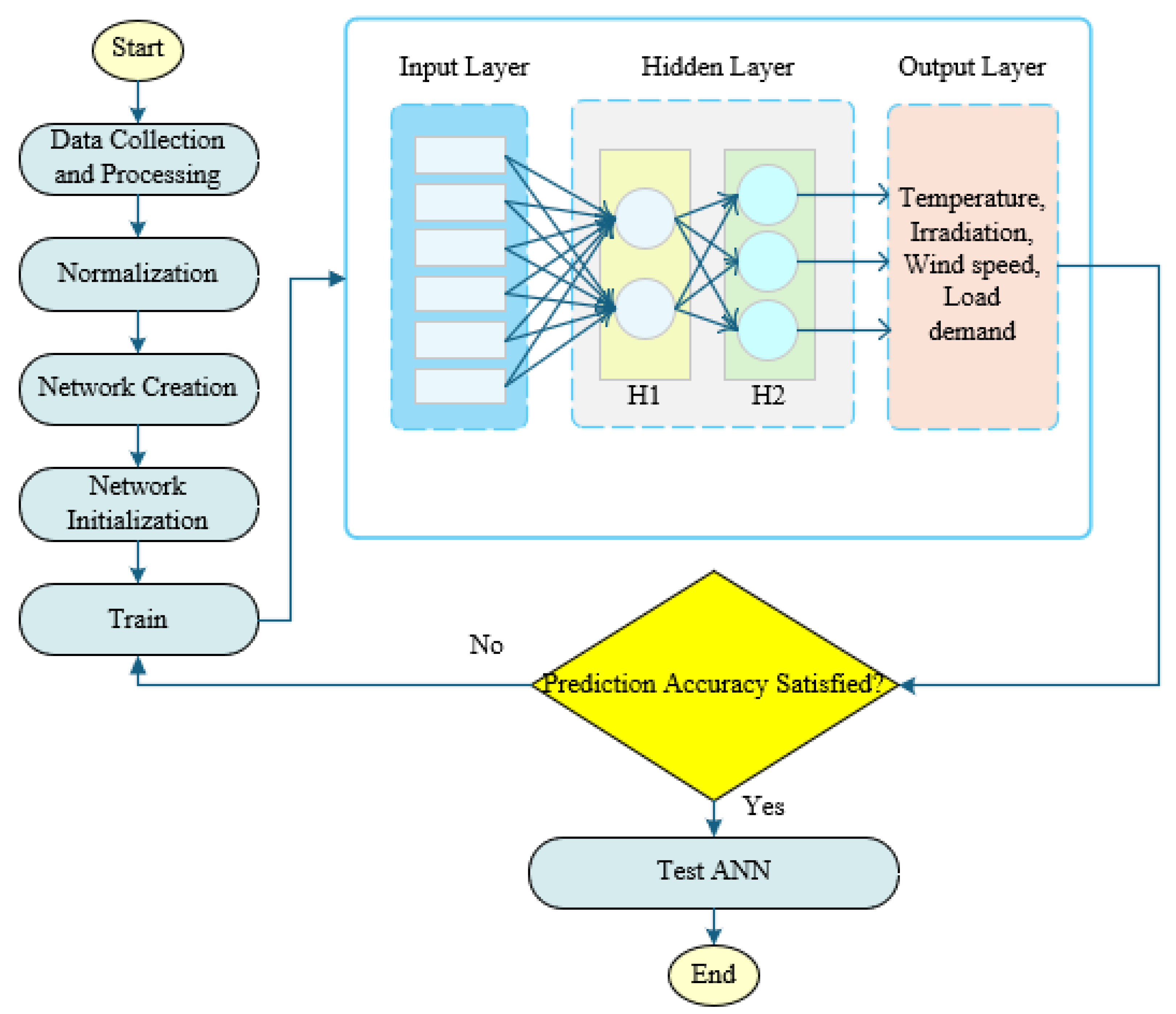
Figure 2.
ANN architecture for the prediction.
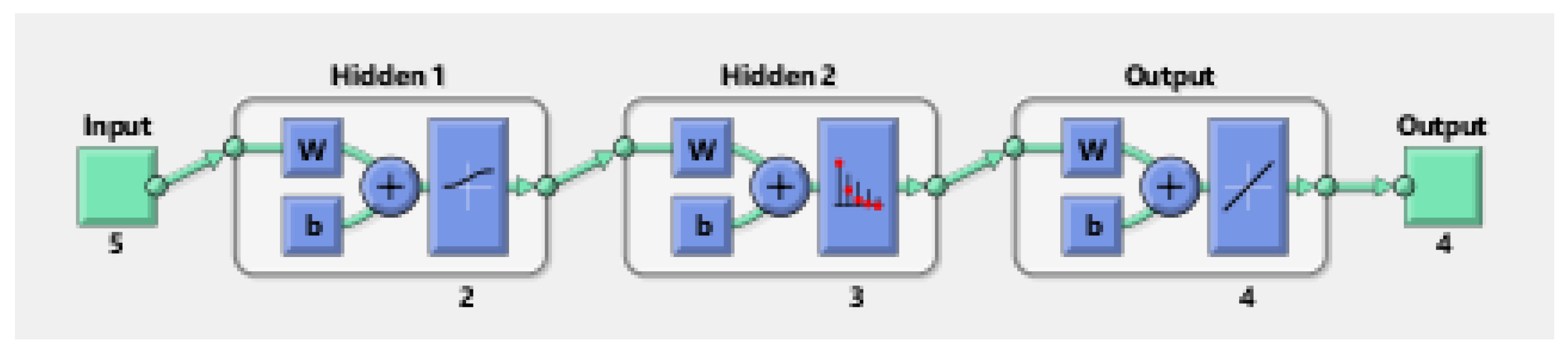
Figure 3.
Flowchart of the proposed MLP-ANN.
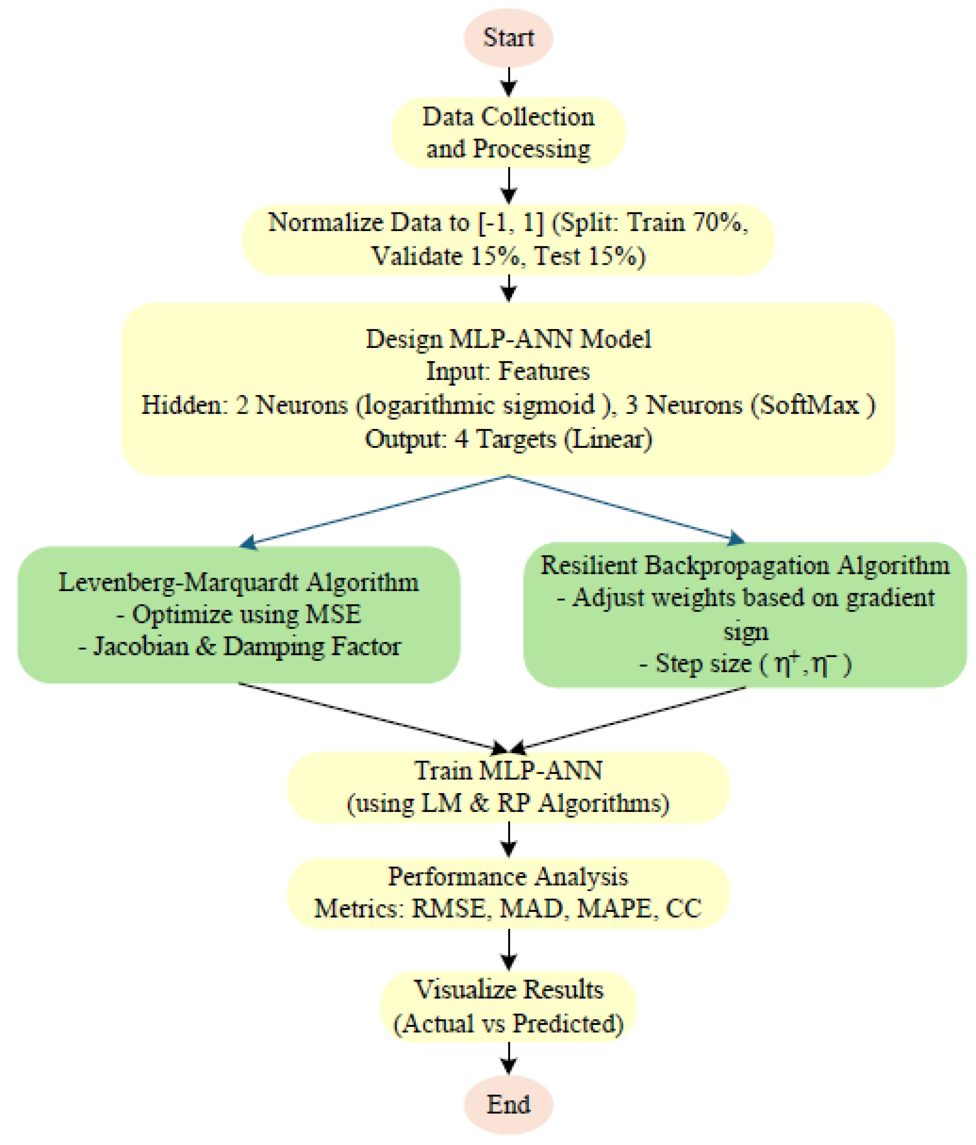
Figure 4.
Updating a cheetah’s position using the proposed strategy selection mechanism in MCO.
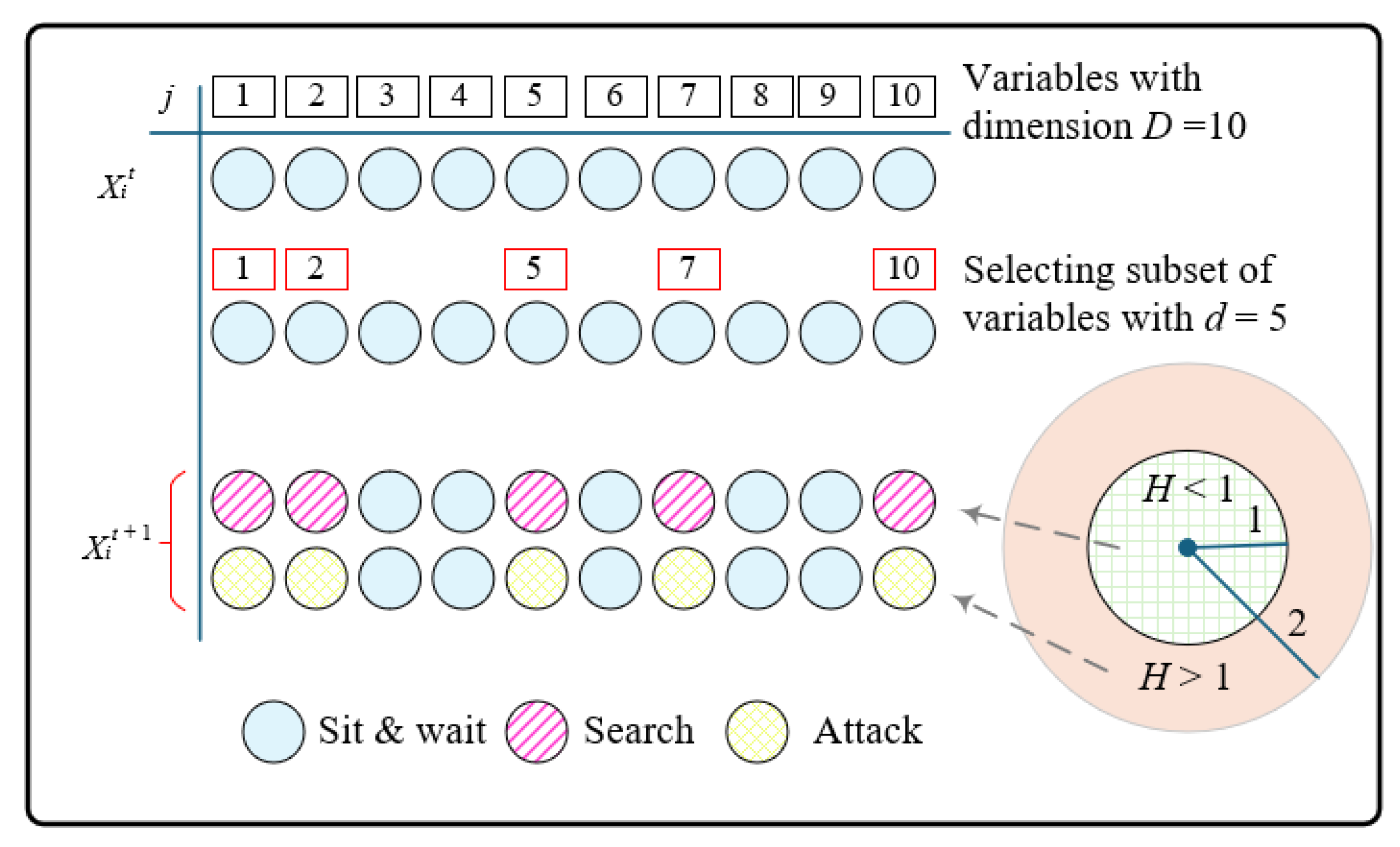
Figure 5.
Representation of EMS.
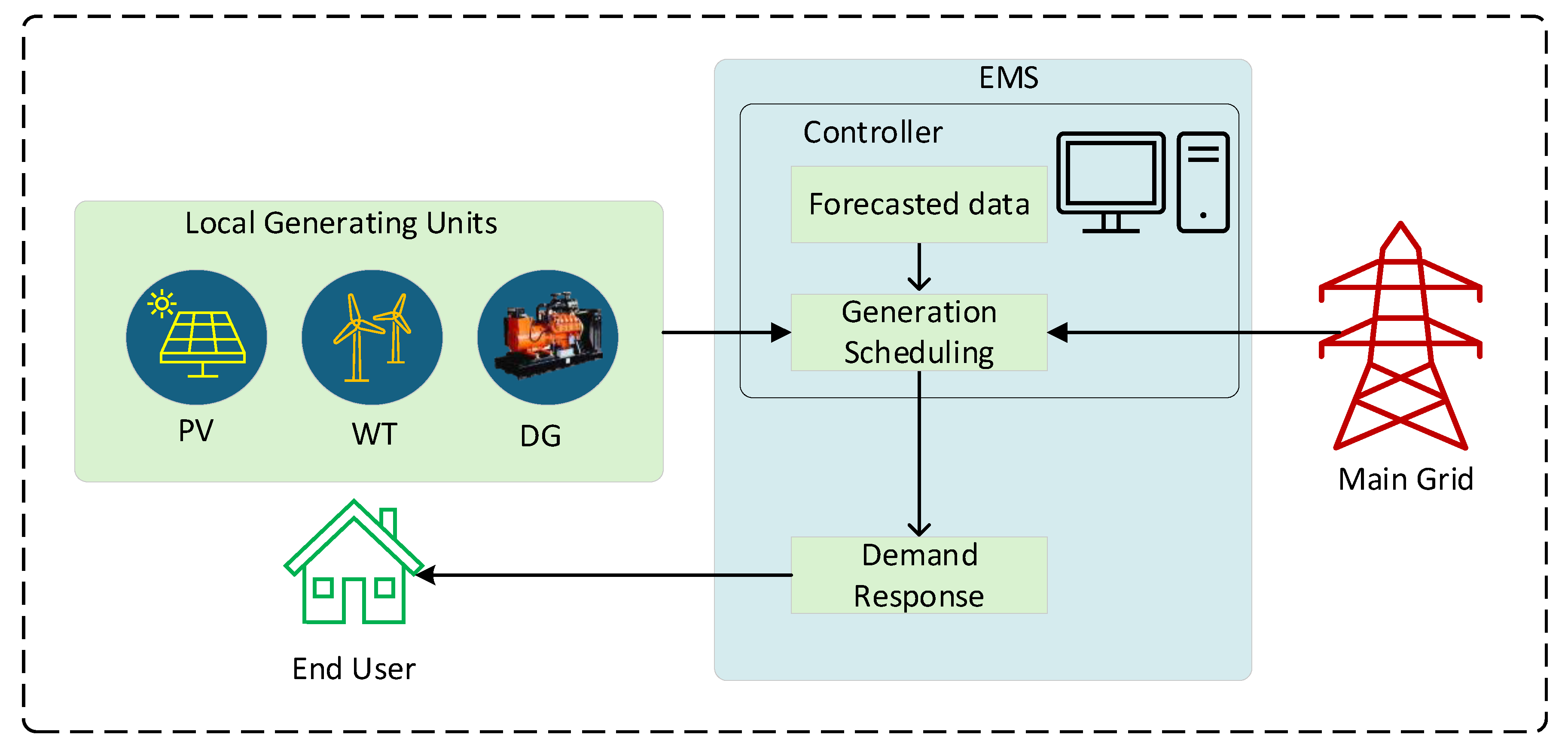
Figure 6.
Flowchart of the proposed MLP-ANN-based MCO for optimal EMS problems.
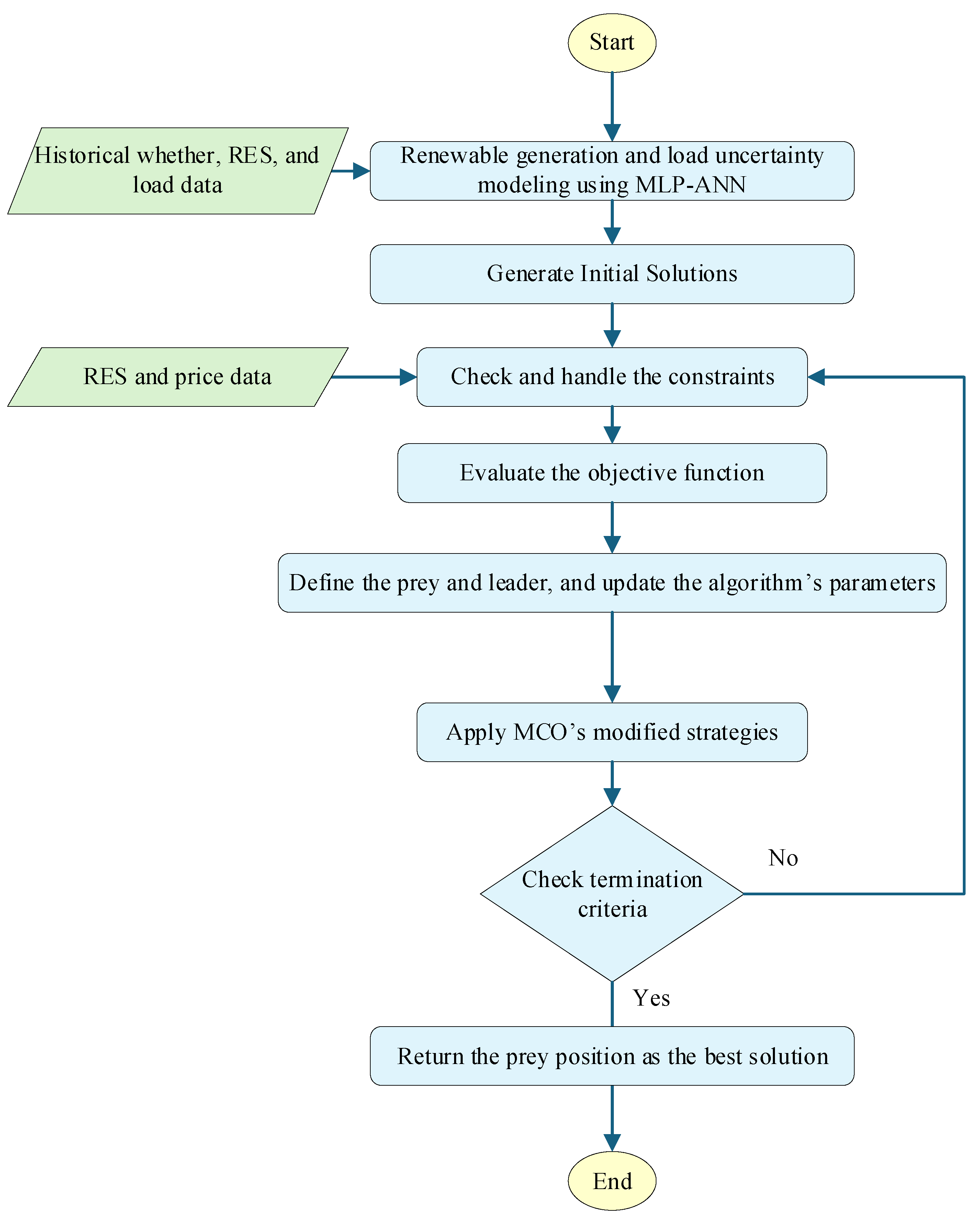
Figure 7.
Flowchart for implementation of the proposed energy management system.
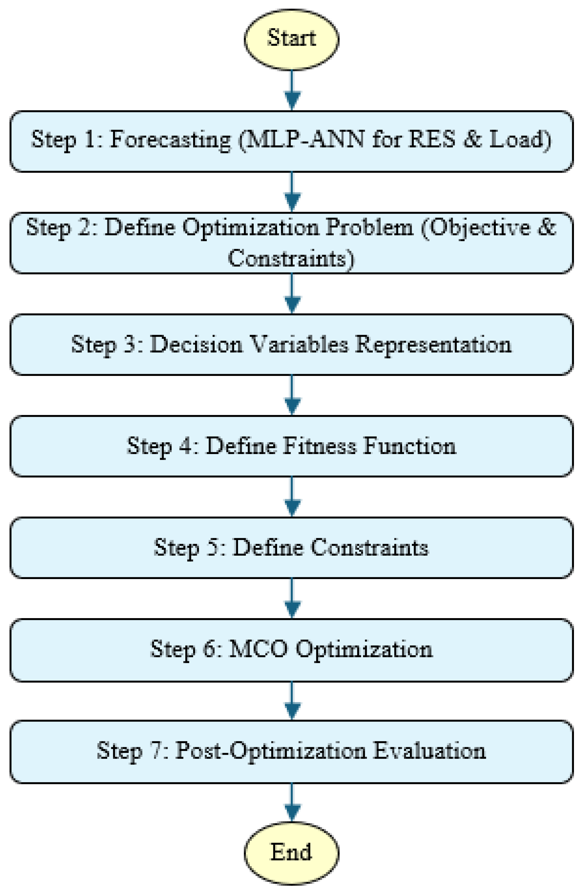
Figure 8.
Microgrid test system.
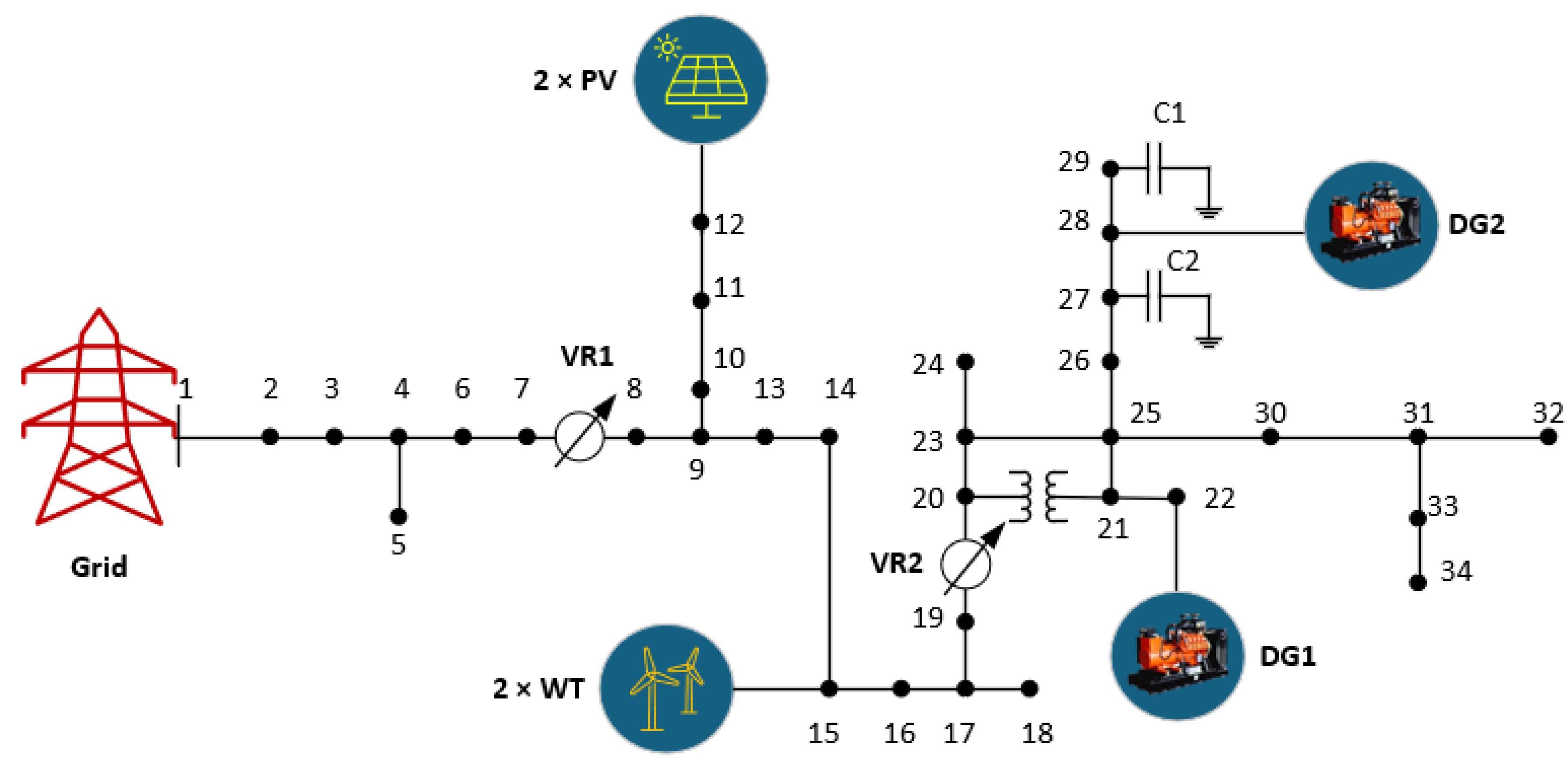
Figure 9.
Predicted solar Irradiation (a), Temperature (b), wind speed (c), and demand (d) for LM and RP.
Figure 9.
Predicted solar Irradiation (a), Temperature (b), wind speed (c), and demand (d) for LM and RP.
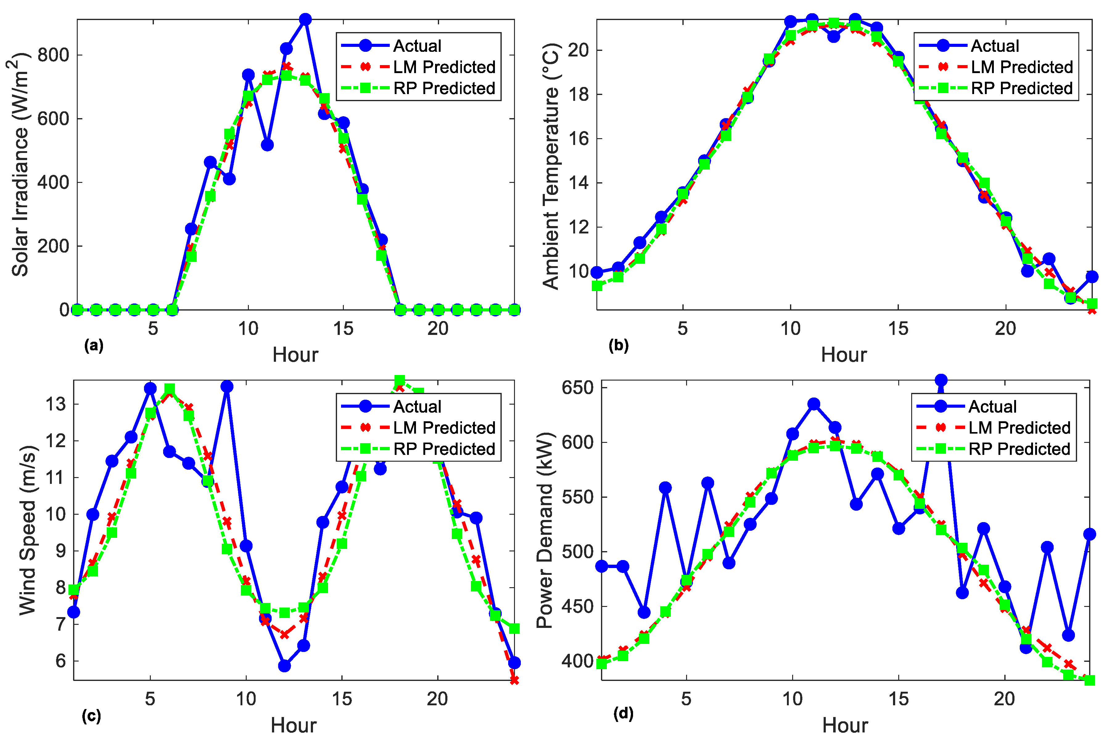
Figure 10.
Regression analysis for LM.
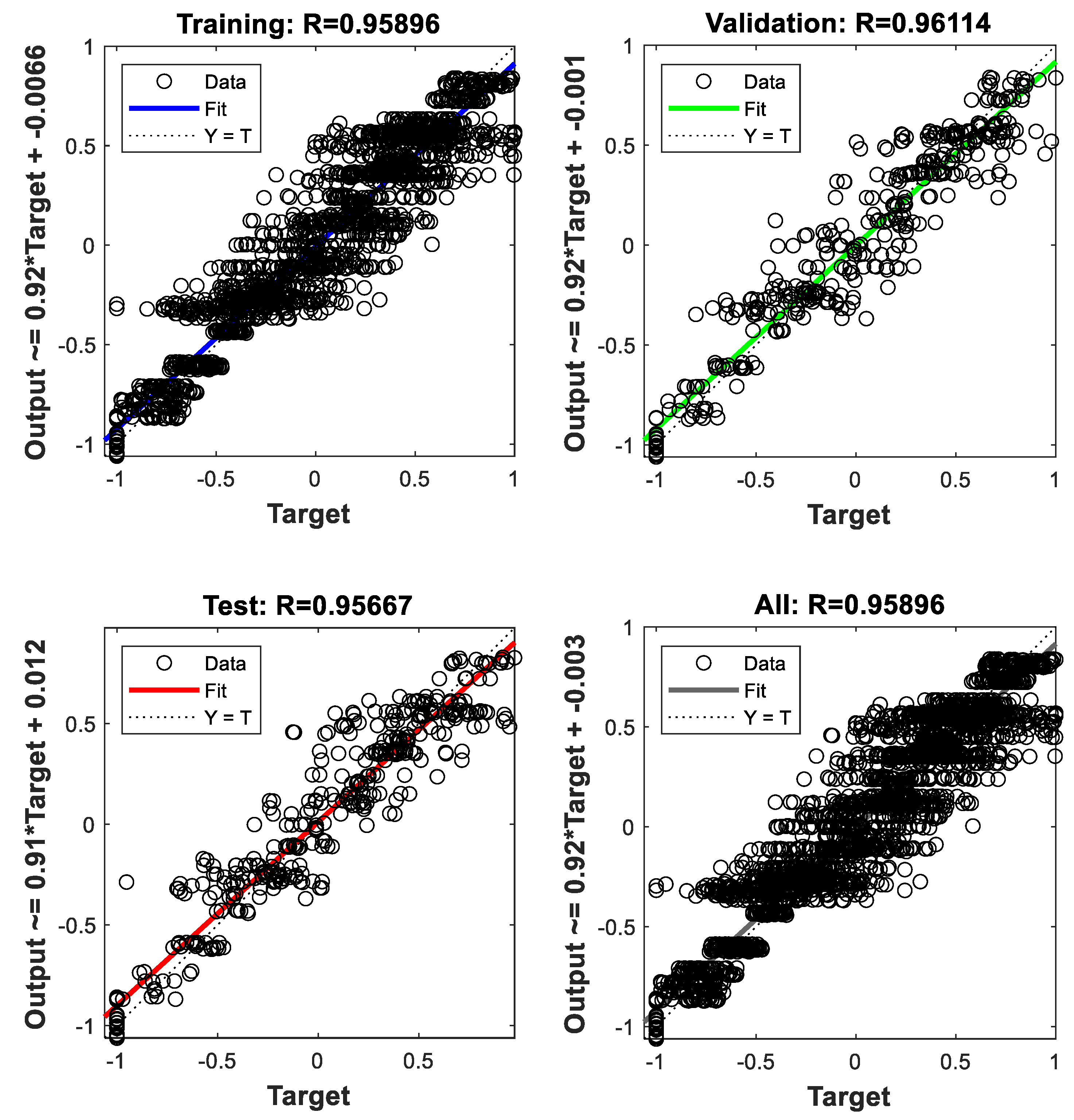
Figure 11.
Regression analysis for RP.
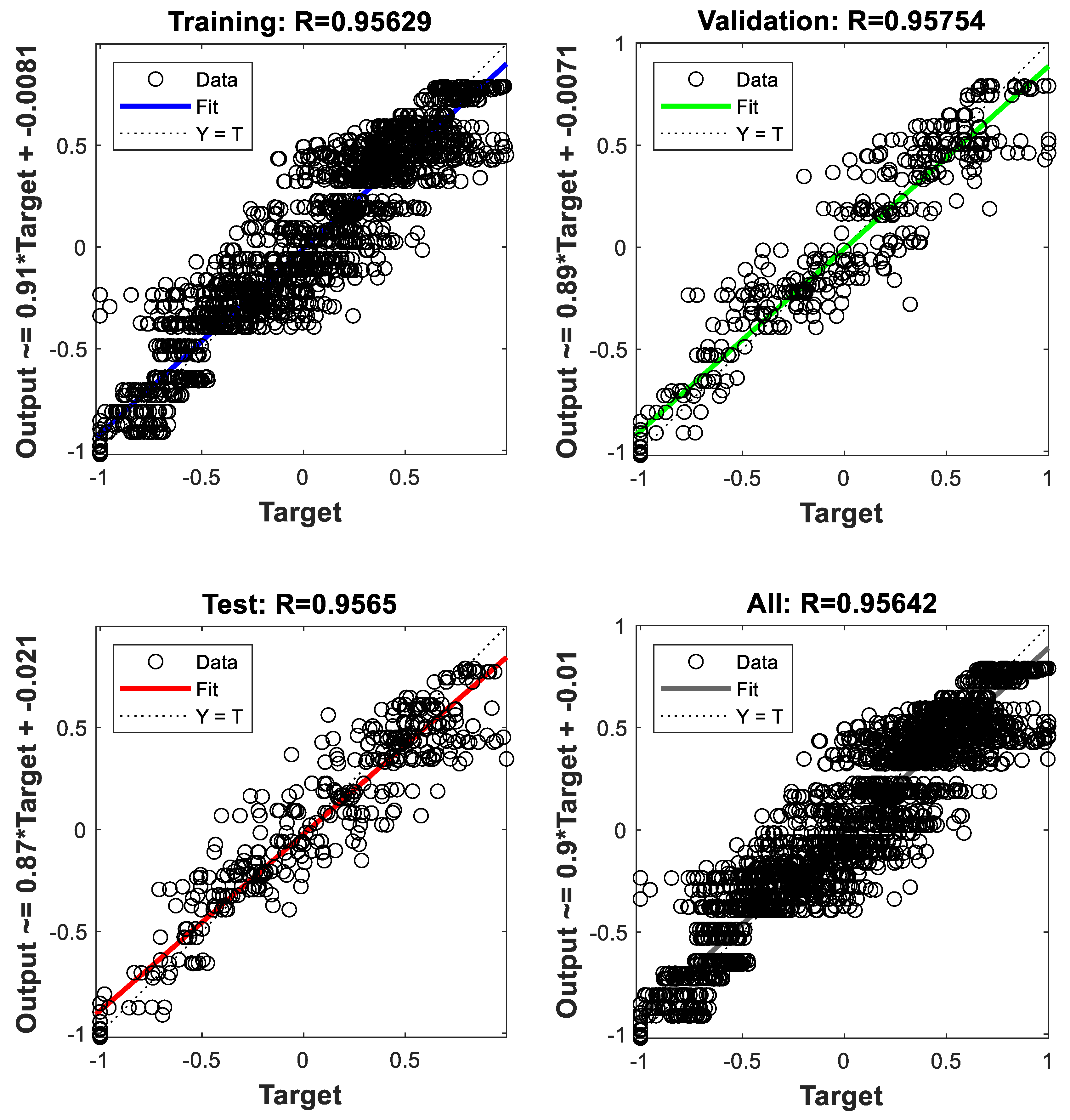
Figure 12.
Optimal microgrid generation scheduling for Case 1.
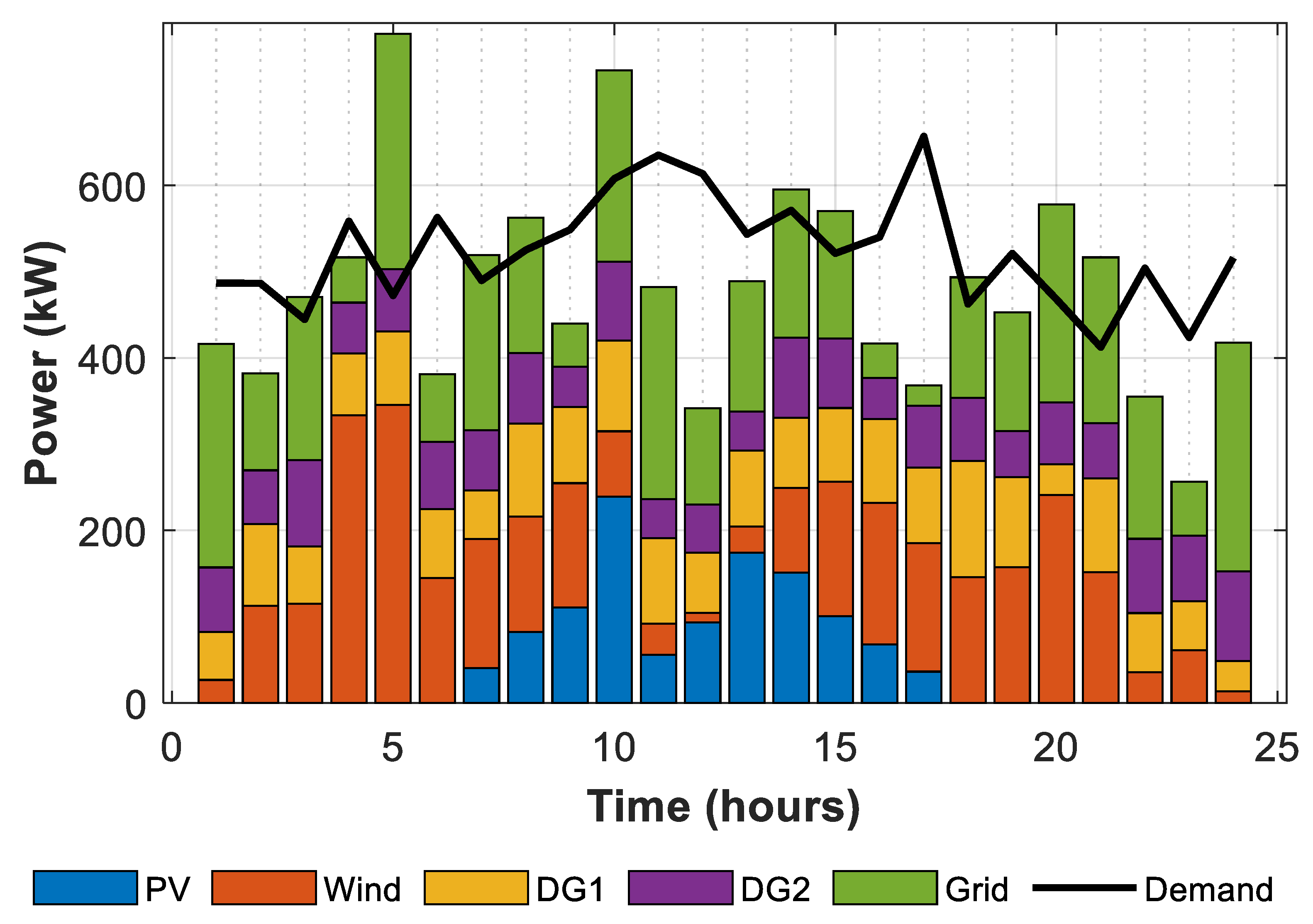
Figure 13.
Hourly shiftable DR program in Case 1.
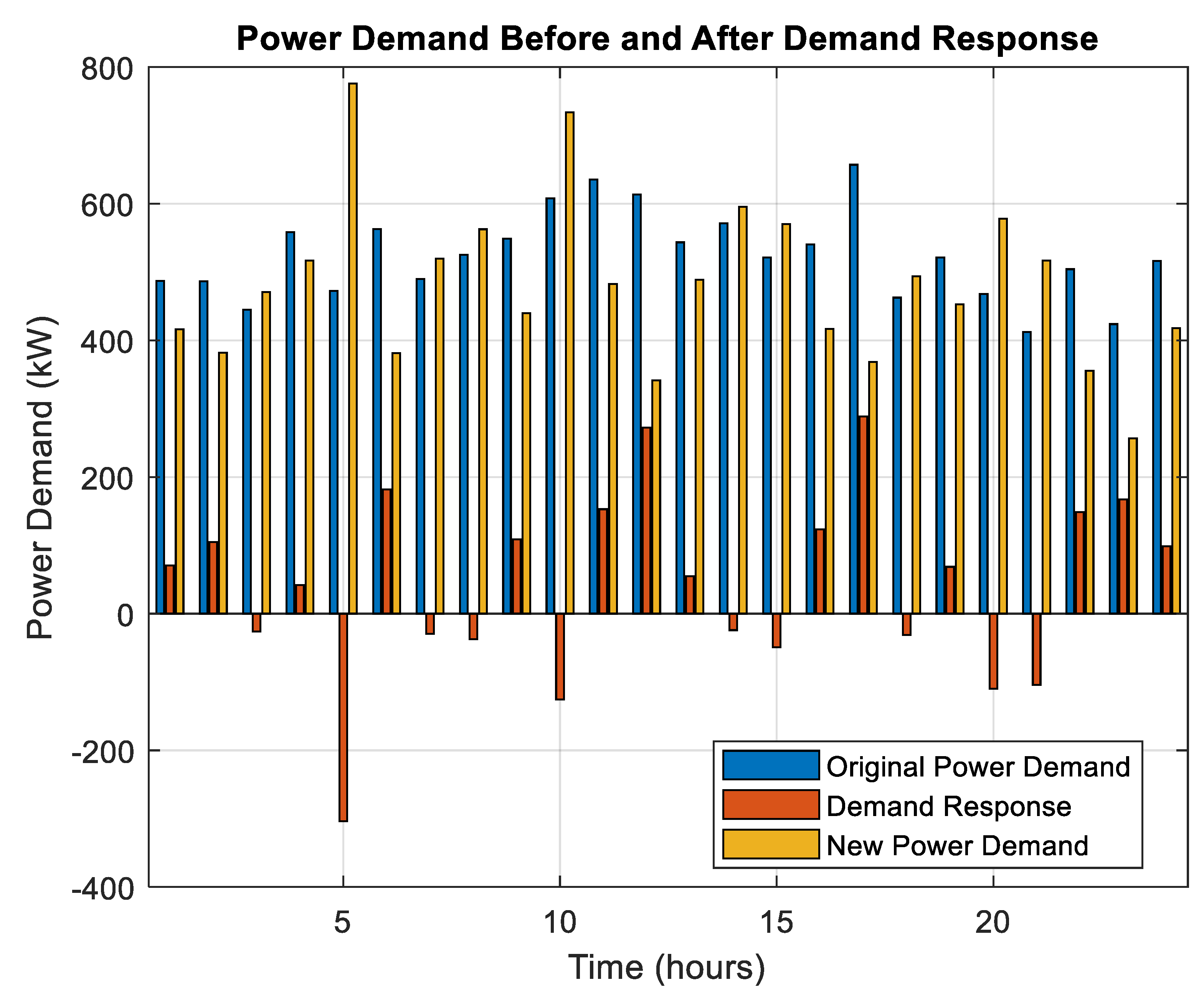
Figure 14.
Optimal microgrid generation scheduling for Case 2.
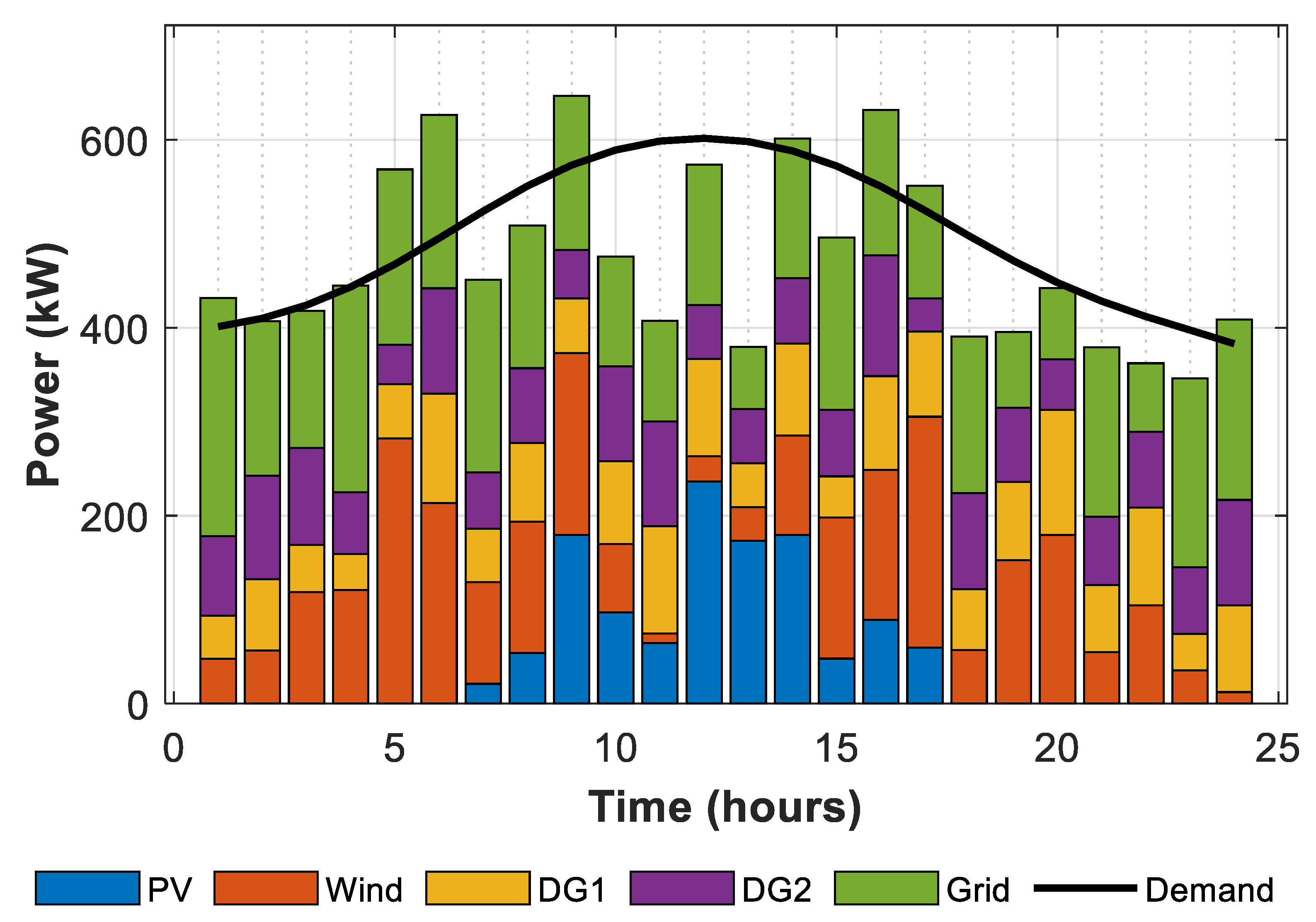
Figure 15.
Hourly shiftable DR program in Case 2.
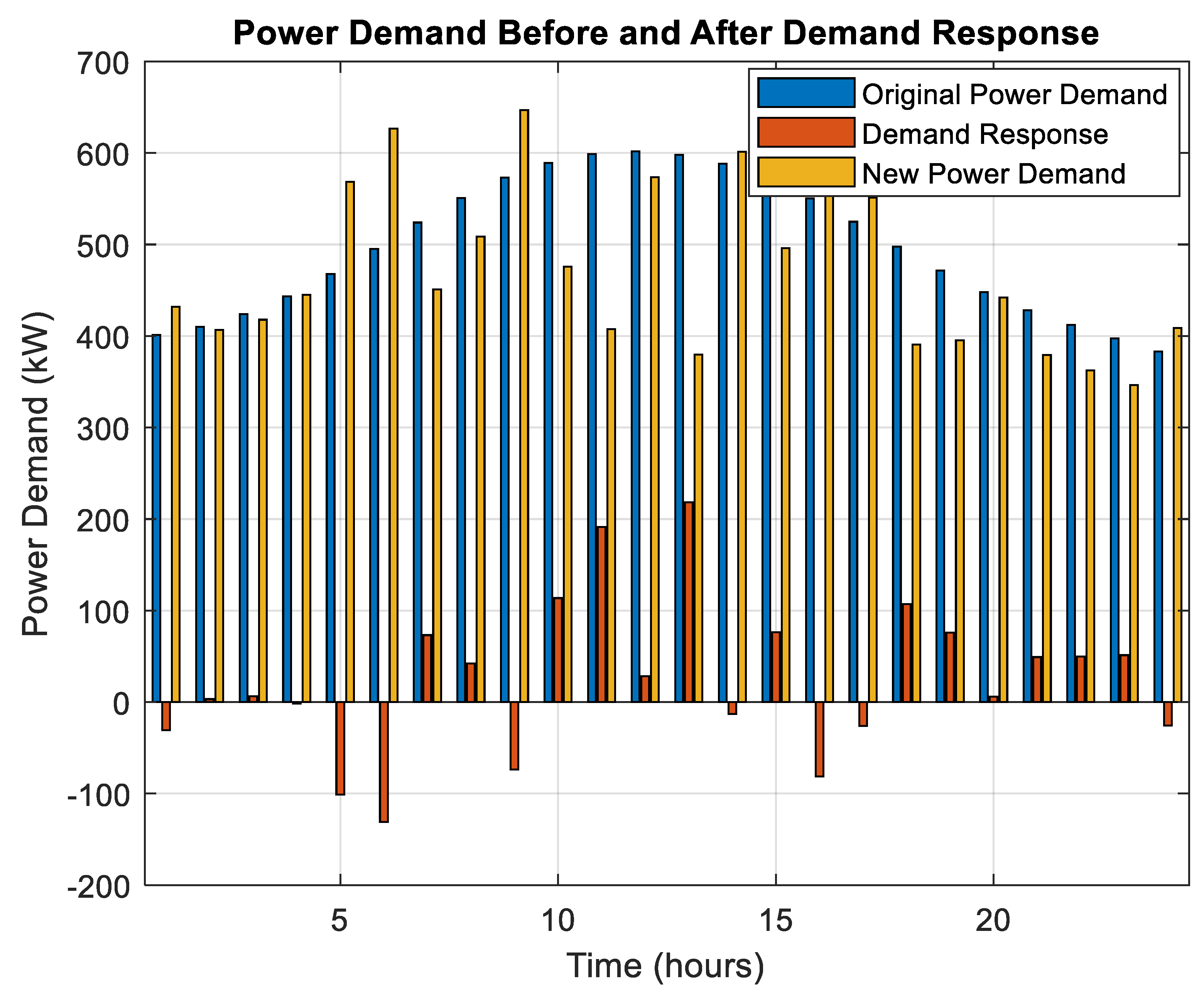
Figure 16.
Optimal microgrid generation scheduling for Case 3.
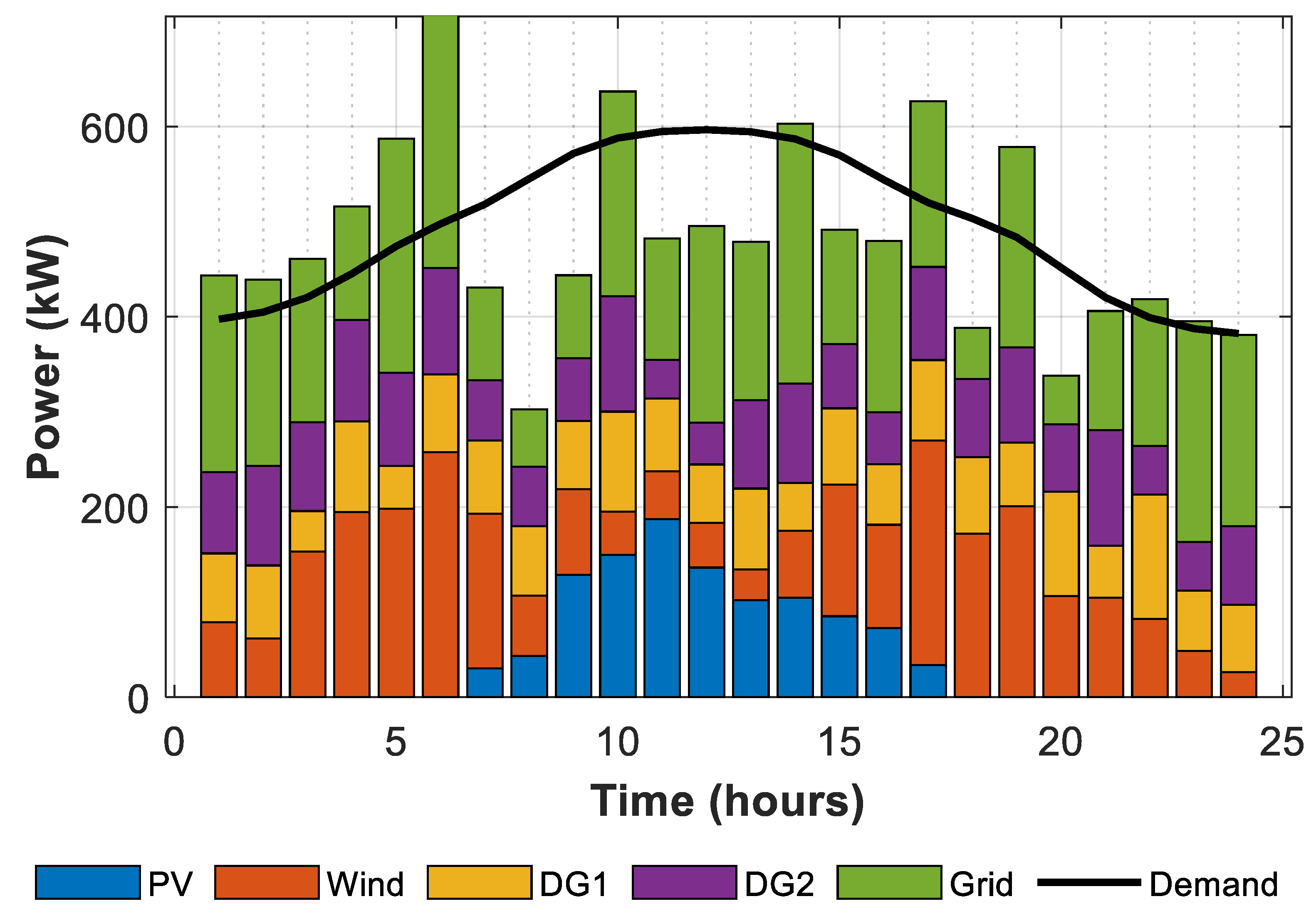
Figure 17.
Hourly shiftable DR program in Case 3.
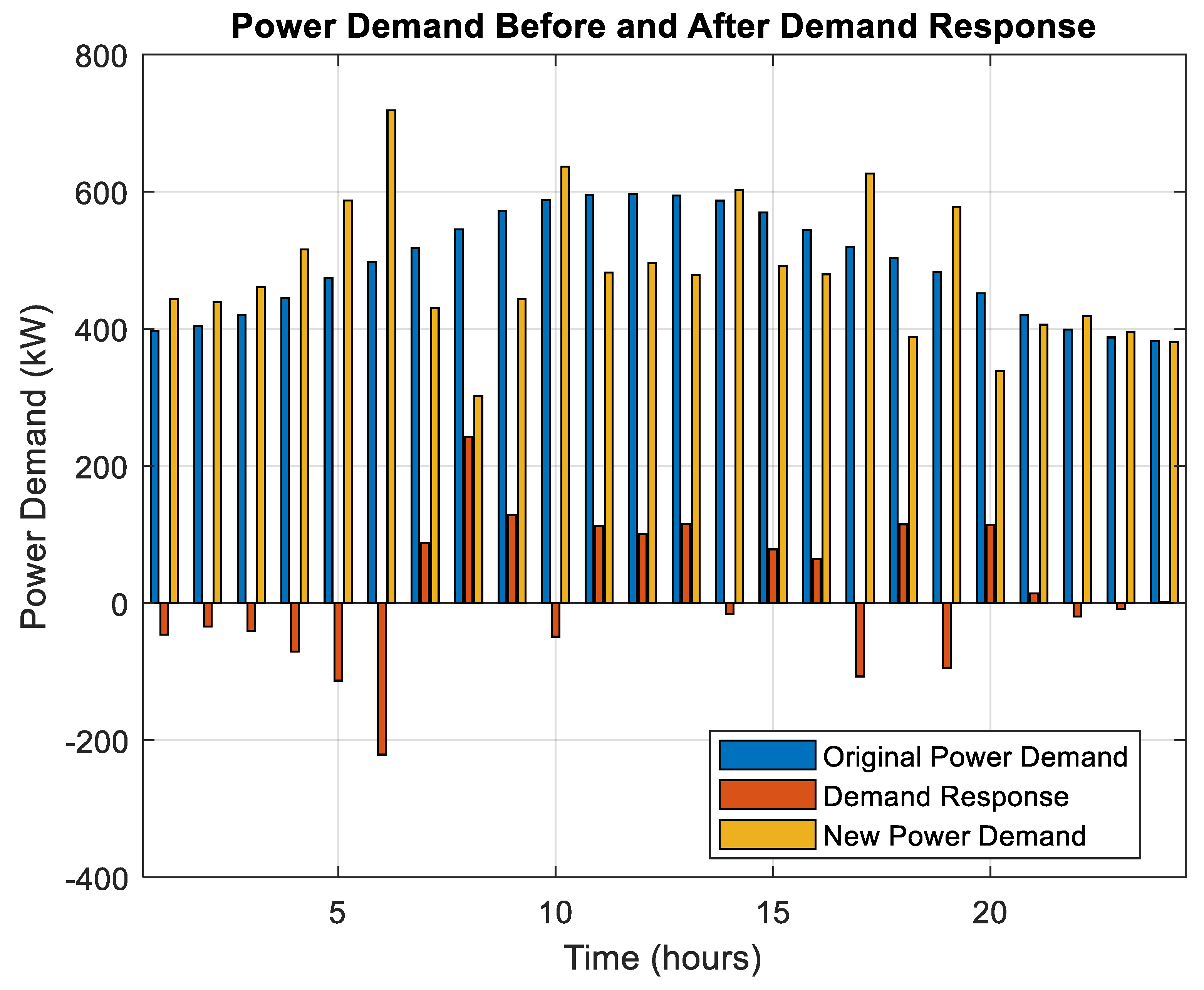
Figure 18.
Convergence curves of the best fitness values obtained using comparative algorithms in Case 1.
Figure 18.
Convergence curves of the best fitness values obtained using comparative algorithms in Case 1.
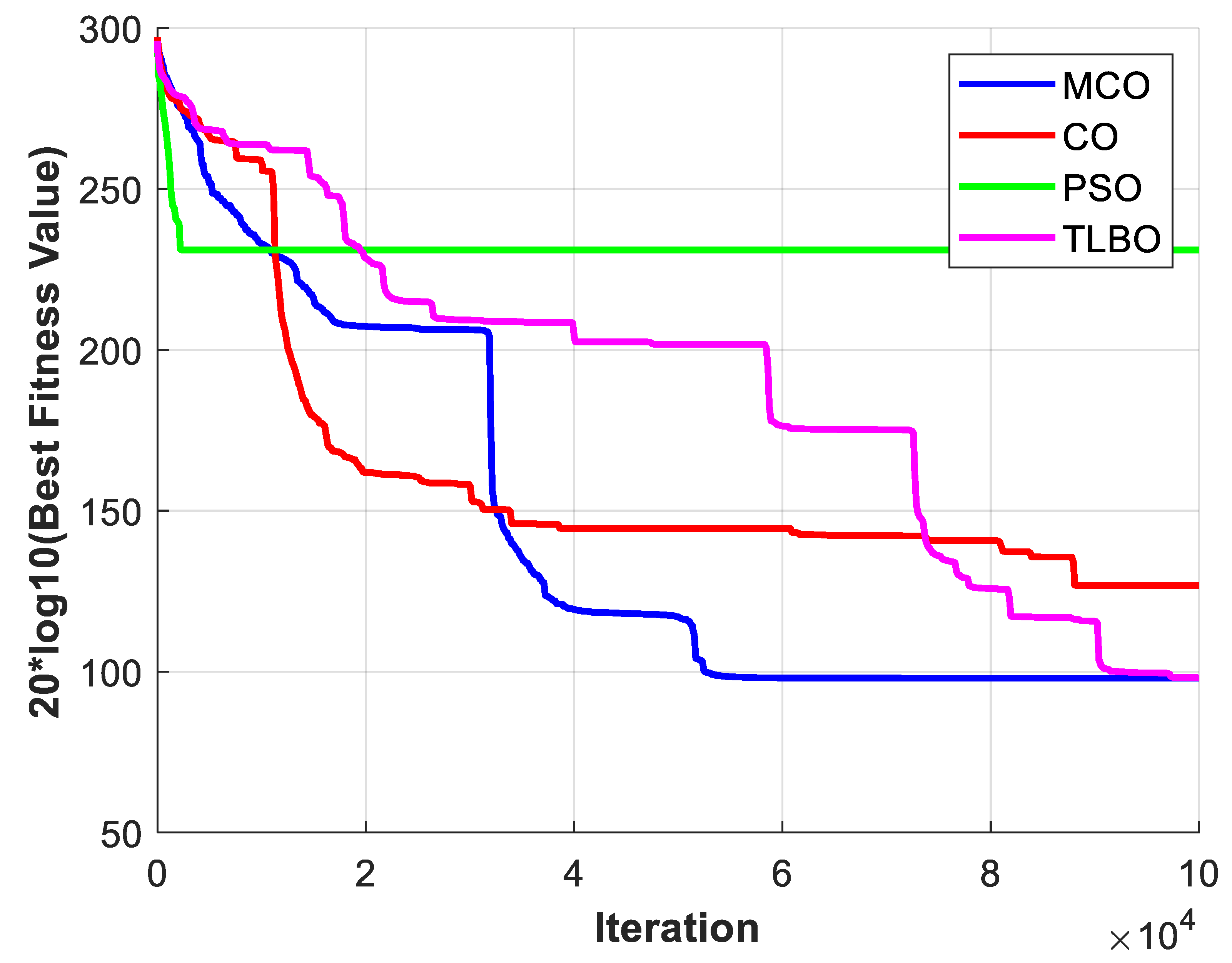
Figure 19.
Convergence curves of the best fitness values obtained using comparative algorithms in Case 2.
Figure 19.
Convergence curves of the best fitness values obtained using comparative algorithms in Case 2.
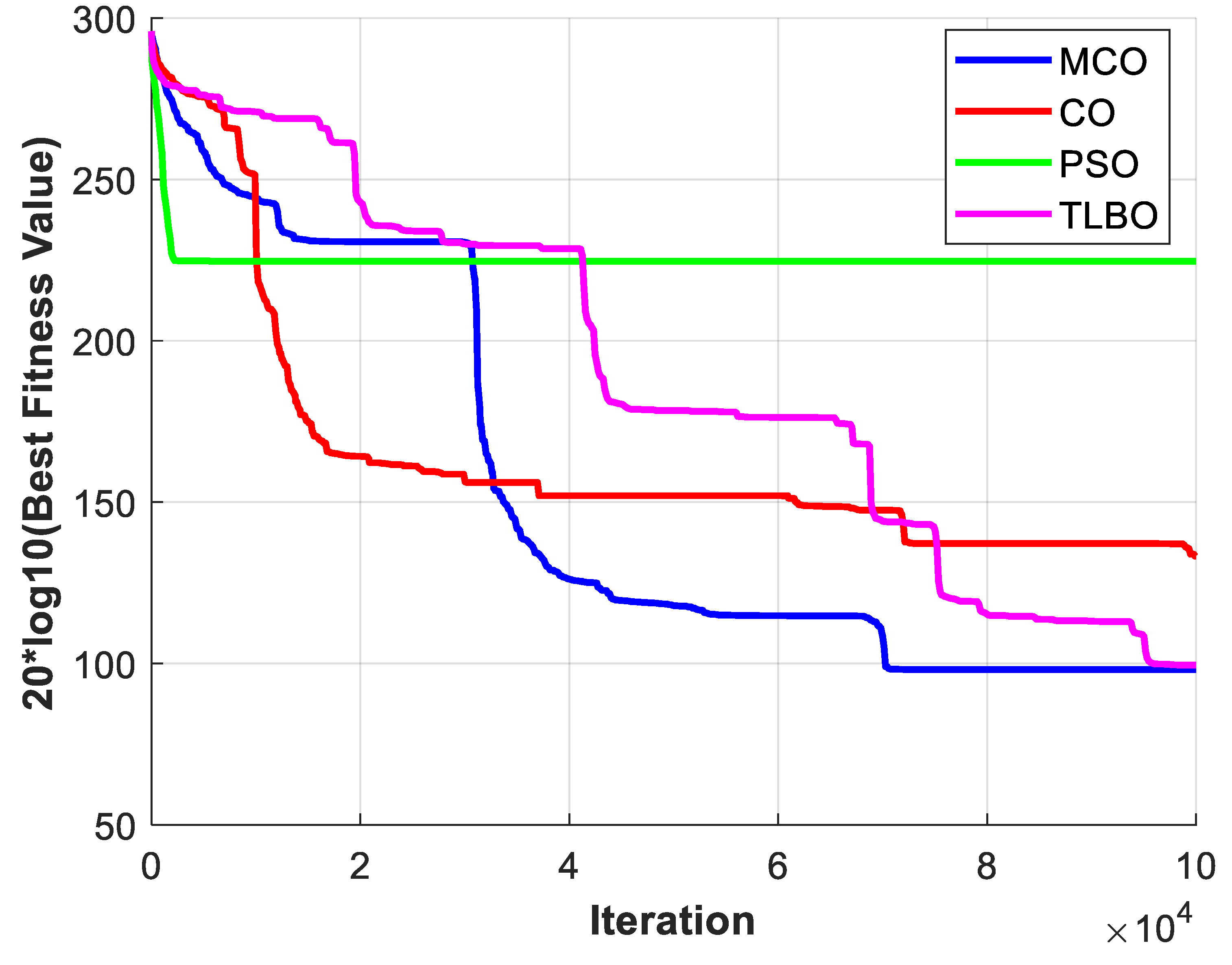
Figure 20.
Convergence curves of the best fitness values obtained using comparative algorithms in Case 3.
Figure 20.
Convergence curves of the best fitness values obtained using comparative algorithms in Case 3.
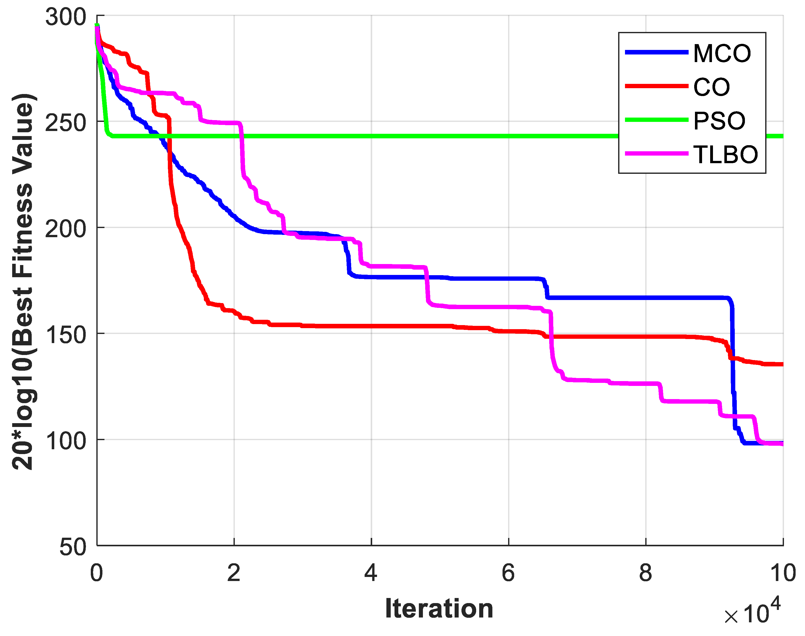

Table 1.
Evaluation metrics for the LM and RP.
| Model | LM | RP | ||||||
|---|---|---|---|---|---|---|---|---|
| Variable | CC | RMSE | MAD | MAPE (%) | CC | RMSE | MAD | MAPE (%) |
| Solar Irradiance | 0.97 | 73.21 | 41.38 | 8.22 | 0.97 | 80.27 | 46.79 | 9.84 |
| Ambient Temperature | 0.99 | 0.50 | 0.41 | 3.18 | 0.99 | 0.71 | 0.62 | 4.55 |
| Wind Speed | 0.88 | 1.18 | 0.92 | 8.63 | 0.82 | 1.38 | 1.08 | 10.78 |
| Power Demand | 0.68 | 62.73 | 49.62 | 9.39 | 0.66 | 62.23 | 48.89 | 9.19 |
Table 2.
Total power generation in the case studies.
| Case# | Gird (kW) | Local gen. (kW) | DR_total(kW) |
|---|---|---|---|
| Case1 | 3680.001456 | 7850.774091 | 1041.677698 |
| Case2 | 3690.546699 | 7653.857775 | 607.1113135 |
| Case3 | 3943.648099 | 7598.336085 | 355.9692446 |
Table 3.
Operation costs (USD/h) of the generation sources in the cases.
| time (h) | wo/opt | Case 1 | Case 2 | Case 3 |
|---|---|---|---|---|
| 1 | 4016.49901 | 2791.127 | 2775.326 | 3370.753 |
| 2 | 4012.299966 | 3380.883 | 3957.249 | 3854.598 |
| 3 | 3415.209351 | 3547.918 | 3265.85 | 2886.221 |
| 4 | 5514.428394 | 2822.845 | 2223.335 | 4311.081 |
| 5 | 3715.604693 | 3372.593 | 2156.397 | 3041.558 |
| 6 | 5605.418322 | 3399.249 | 4880.023 | 4128.463 |
| 7 | 4078.380805 | 2706.178 | 2514.636 | 3025.003 |
| 8 | 4845.054157 | 4082.725 | 3523.624 | 2926.634 |
| 9 | 5337.48599 | 2928.058 | 2390.988 | 2974.416 |
| 10 | 5745.957024 | 4246.864 | 4058.731 | 4853.323 |
| 11 | 5748.957753 | 3155.872 | 4837.422 | 2558.217 |
| 12 | 5746.599395 | 2729.704 | 3493.648 | 2308.117 |
| 13 | 5228.080859 | 2897.346 | 2268.99 | 3829.498 |
| 14 | 5741.948459 | 3743.277 | 3625.395 | 3336.166 |
| 15 | 4764.706964 | 3574.969 | 2475.976 | 3200.479 |
| 16 | 5157.624 | 3135.079 | 4891.306 | 2574.407 |
| 17 | 5751.342471 | 3441.607 | 2745.905 | 3921.388 |
| 18 | 3538.947464 | 4487.293 | 3580.845 | 3492.784 |
| 19 | 4736.03933 | 3409.708 | 3482.03 | 3563.465 |
| 20 | 3625.319983 | 2303.714 | 4031.57 | 3875.136 |
| 21 | 2456.36054 | 3701.873 | 3089.849 | 3743.393 |
| 22 | 4377.830472 | 3308.831 | 3951.49 | 3917.054 |
| 23 | 2700.935559 | 2841.413 | 2337.571 | 2458.137 |
| 24 | 4627.31293 | 2961.224 | 4351.358 | 3271.488 |
| Total cost | 110488.3439 | 78970.35 | 80909.51 | 81421.78 |
Table 4.
Comparison of operational cost reduction between the proposed method and the state-of-the-art results.
Table 4.
Comparison of operational cost reduction between the proposed method and the state-of-the-art results.
| method | Uncertainty | Operating cost reduction (%) |
|---|---|---|
| [34] | PV uncertainty | 15.6% |
| [35] | Not consider | 5% |
| [36] | Wind uncertainty (10%) | 27% |
| [12] | Price uncertainty | 16% |
| [2] | 11% PV uncertainty, 10% wind uncertainty | 23% |
| Case 2 | Forecasted Load and RES with LM | 26.8% |
| Case 3 | Forecasted Load and RES with RP | 26.3% |
Table 5.
Statistical results of optimal EMS using different algorithms in case studies.
| Case# | Metric | MCO | CO | PSO | TLBO |
|---|---|---|---|---|---|
| 1 | min | 7.90E+04 | 8.63E+05 | 8.08E+06 | 2.32E+06 |
| mean | 2.17E+06 | 2.73E+07 | 5.80E+07 | 1.54E+07 | |
| max | 3.55E+11 | 3.71E+12 | 2.09E+13 | 4.33E+12 | |
| SD | 8.02E+04 | 1.76E+12 | 1.96E+13 | 4.67E+12 | |
| 2 | min | 80909.53 | 21894794 | 4.3E+08 | 96116699 |
| mean | 4610438 | 26485154 | 58549038 | 14268439 | |
| max | 1.7E+11 | 3.16E+12 | 1.19E+13 | 2.98E+12 | |
| SD | 94543.7 | 3.18E+12 | 2.21E+13 | 5.92E+12 | |
| 3 | min | 81490.88 | 134489.5 | 824219.3 | 168877.8 |
| mean | 5944093 | 24715388 | 41816119 | 11115255 | |
| max | 1.43E+12 | 4.9E+12 | 2.65E+13 | 5.79E+12 | |
| SD | 78730.35 | 5.87E+11 | 4.13E+12 | 1.34E+12 |
Disclaimer/Publisher’s Note: The statements, opinions and data contained in all publications are solely those of the individual author(s) and contributor(s) and not of MDPI and/or the editor(s). MDPI and/or the editor(s) disclaim responsibility for any injury to people or property resulting from any ideas, methods, instructions or products referred to in the content. |
© 2025 by the authors. Licensee MDPI, Basel, Switzerland. This article is an open access article distributed under the terms and conditions of the Creative Commons Attribution (CC BY) license (http://creativecommons.org/licenses/by/4.0/).
Copyright: This open access article is published under a Creative Commons CC BY 4.0 license, which permit the free download, distribution, and reuse, provided that the author and preprint are cited in any reuse.


