Submitted:
02 July 2025
Posted:
04 July 2025
You are already at the latest version
Abstract
: Air transportation industry is challenged to address airport curbside delay problem that affects landside service quality and can potentially impact check-in operation. Methodological advances guided by industry requirements are needed to support curbside improvement studies. Existing methods require verification of assumptions prior to application or need expensive surveys to acquire data for use in microsimulations. A probability-based macrosimulation method is advanced for the evaluation of level of service and capacity of the curbside processor. Following problem definition and literature review, the theoretical foundation of the method is described as the simulation of the stochastic balance of demand and available curb space for unloading/loading task. The method meets the planning and operation requirements with ability to analyse conditions commonly experienced at the curb area. Example applications illustrate the flexibility of the method in evaluating existing as well as planned facilities of diverse designs and sizes. The developed method can contribute to curbside processor delay reduction and due to the macroscopic nature of the method, the data requirements can be met by an airport authority without costly surveys.
Keywords:
airport curbside
; level of service
; capacity
; evaluation
; stochastic
; macrosimulation
; Montecarlo
; operation
; planning
1. Introduction
Airports are accessed by regional multimodal transportation systems, comprising mainly of road modes and at some airports rail-based service is provided [1,2]. Landside curb area of the airport is of specific interest in this research. It is used by private vehicles, shuttle services, taxis, limousines, and shared mobility services provided by Transportation Network Companies (TNCs). The curb for the passenger terminal building is the most convenient location for drop-off and pick-up tasks. Airport roads are designed to serve curb areas, parking, and other facilities. To help prevent vehicles occupying curb spaces while waiting for passengers, cell phone holding areas are provided at some airports. Examples are O’hare in Chicago [3] and Toronto Pearson Airport [4].
Taxis and limousines use waiting areas when not serving passengers so that these do not occupy scarce curb spaces in front of terminal building. A relatively new consideration is the need for TNCs (e.g., Uber) to serve the air traveling public. Their vehicles are allowed to wait in a designated location at the airport before moving to a curbside spot for serving arriving customers [5,6,7]. However, at some airports with severe shortage of curb spaces in front of terminal building, the customers are expected to walk to the waiting TNC vehicles in the designated location [8].
Given the growth in air travel and the dominance of the automobile for airport access, methodological advances are needed to predict if user expectation of acceptable quality of service can be met during the unloading/loading operation at the curbside. For assessing the performance of existing curbside facilities as well as for planning improvements, airport planners, operations personnel, and managers can be assisted with new research in curbside level of service (LOS).
Over the years, research studies have contributed knowledge on LOS and capacity of processors in the terminal building (e.g., check-in, baggage collection) [9,10,11,12,13,14,15]. Correia and Wirasinghe reviewed these as well as other sources of information on approaches for evaluation of LOS at airport passenger terminals [16]. But only a few research studies have been reported that focus on the LOS of the curb part of the airport. These are reviewed in a later section of this paper.
The LOS is an indicator of the quality of service experienced by travellers. According to the International Air Transport Association (IATA), the LOS as a basic airport planning tool can be used for many purposes, including processor assessment, capacity analysis, and planning and design of new facilities [17]. To be useful, a qualitative indicator of LOS is supported with a quantitative measure such as delay time.
In the case of airport roads that connect with the terminal curb area, the Highway Capacity Manual (HCM), published by the Transportation Research Board (TRB), can be used for assessing the service quality provided to users [18]. A logical measure for the LOS offered by the curbside is the probability of accessing space and corresponding delay. For airport planning and operations, the relationship between LOS and capacity of the curbside processor should be known. The capacity of the curbside facility can be viewed as the maximum unloading/loading events per selected time duration (e.g., an hour), without causing a functional breakdown of operations. At the present state of knowledge, the quantitative criteria (i.e., delay) for curbside LOS grades, including capacity level operation, are not well developed.
This paper contributes a probability-based macrosimulation method for evaluating the LOS offered to curb space users. The developed method can support operations and planning tasks. The following sections of the paper cover the research approach, model formulation, macrosimulation method, LOS, delay index, robustness verification, applications, discussion, and conclusions.
2. Research Approach
In this section, the need for a new method is explained for addressing curbside planning and operation problems. Existing methods are reviewed, and requirements are defined that are to be met by a new method.
2.1. Curbside Planning and Operation Problems
Bud et al. [19] investigated key issues affecting airport ground access. At the landside system level, curb area operation is challenging during high demand periods [20,21,22]. Depending upon the airport size, the configuration of curb space varies much. For a small airport or a terminal within an airport with multiple terminals, one curbside lane is usually sufficient for departing as well as arriving passengers, supplemented by another two lanes used for manoeuvring and through movements. If allowed by the airport authority (e.g., in Beijing, China, Capital Airport Terminal 3), the lane next to the curb lane may be used for unloading/loading tasks during peak conditions (called “double parking”) [23].
According to the National Academy of Sciences, Engineering and Medicine (NAS), a four-lane cross section is commonly used at airports that allow double parking during peak times [24]. The two outer lanes enable manoeuvring and through movements. At large airports, two parallel curb fronts (i.e., inner and outer curb lanes) are provided, separated by a pedestrian island (Figure 1). Some passenger terminals have the lane configuration of the curbside processor shown in Figure 1, but with three lanes in each parallel curbfront. The arrival curbfront of Pearson Airport Terminal 1 in Toronto is an example [25].
For efficient operations, the curbfront traffic is usually separated into passenger cars and commercial vehicles (e.g., parking shuttles, rental car shuttles, hotel/motel shuttles, taxis, limousines, etc.). Depending upon the airport policy, the lanes closest to the terminal building can be used by larger vehicles such as shuttle buses and the outer curb lanes are used for private vehicles. Examples are the Toronto Pearson Airport [25] and Los Angeles International Airport [26]. Many passenger terminals are designed with two-level curbfronts. The upper level is typically used for departing passengers and the lower level is best suited for arriving passengers who collect their bags before leaving the airport (e.g., International Airport Authority Ottawa) [27]. Other design configurations are used for specialized applications such as dedicated curb spaces for various vehicle types and functions. An example is accessible vehicle unloading/loading [28,29].
As the driver of a vehicle arrives in the vicinity of the passenger terminal building, the driver follows instructions regarding inner curb or outer curb and decides to move to an available curb space. As noted above, at some airports, inner curb lanes are reserved for shuttles, etc., and private vehicles use outer curb lanes. In a future scenario, if connected and automated vehicles are used for delivering passengers and meeting arriving passengers, an automated curb operation system will guide vehicles to available curb spaces. In situations when demand for curb use exceeds the availability of curb spaces, vehicles form queues and wait for available curb spaces.
Th design of curbside and travel lanes (as shown in Figure 1) prevents vehicle interaction. Vehicles wait in their selected lanes and when an unoccupied space is detected, they use a travel lane to approach the vacant space. The occupancy time obtained from a survey account for simultaneous movements of approaching and exiting vehicles. Also, the survey-based time accounts for time needed for pedestrians to cross lanes.
For the planning and operation tasks, it is necessary to study the dynamics of demand versus supply of curb spaces. Airport authorities and planners need a method that can be used to obtain LOS and associated delay answers without the need for expensive studies.
The number of curb spaces to serve demand for various types of vehicles depends upon vehicle characteristics, unloading/loading operation, and allowed curbfront length. If double parking is allowed during high demand periods, the supply of spaces increases. The time duration for the use of a curb space by a vehicle can be affected by the extent of double parking. A simulation study of Toronto Pearson Airport Terminal 1 arrivals area (with 3 lanes for private vehicle use) applied an average 133 seconds wait time per vehicle to go to the curb space and enter it for the base case and found 150 seconds for the double-parking scenario [30]. The increased wait time is due to double parking.
2.2. Past Research in Curbside Level of Service
Over the years, researchers have used analytical and simulation approaches to assess the performance of the overall landside processors, including the curbside area [31]. However, published research with focus on curbside LOS is scarce. In general, the analytical approaches lack theoretical foundation and validation information is rarely provided. Recent research has applied macroscopic, mesoscopic, and microscopic simulation techniques that provide higher fidelity results on curbside facility performance than analytical methods. Existing macroscopic simulation tools provide performance results, but the validation of the assumptions of queueing theory functions is data- intensive. The microscopic simulation tools provide a high level of detail for each user of the curb but require much data. The mesoscopic simulation technique can provide microscopic level detail of selected variables and macroscopic simulation of other variables for which detailed level of analysis is not warranted [30,32].
2.2.1. Curbside Performance
Braaksma and Mo [33] described effectiveness measures for airport departure curbs. Parizi and Braaksma [34] developed a method that incorporates users’ behaviour for the study of enplaning curbside areas at airports. Their design tool applied the vehicular demand distribution over the doors of the terminal building and outputs include the optimum number of doors, door locations, effective length of the curb, and practical dynamic capacity of the curbside area.
Several Airport Cooperative Research Program (ACRP) reports on terminal planning, design, and operations were published by the NAS in 2010, 2011, and 2019. The ACRP Report 55 [15] scans practices regarding quality of passenger services and spatial planning for airport terminals. The ACRP Synthesis Report 98 [31] provides an overview of simulation options for airport planning.
Volume 1 of ACRP Report 25 serves as a guidebook on terminal curb and roadway requirements [20]. Volume 2 of the ACRP Report 25 describes queueing theory-based spreadsheet models [21]. The ACRP Report 40 presents an overview of analytical and simulation methods [24]. The Quick Analysis Tool for Airport Roadways (QATAR) is described which is intended to quantify curb space utilization under specified demand, lane configuration and associated curb space supply.
The QATAR is structured as a queueing model. The logic of the method assumes infinite calling population, steady state system, Poisson probability distribution of vehicle arrivals, and exponential probability distribution of service times. The ACRP Report 40 [24] also includes an application of a microsimulation method noted in the next section of this paper.
Several macroscopic simulation software is described in the literature. Examples are the discrete simulation tools [35,36], the Terminal, Roadway, and Curbside Simulation (TRACS) [37], the Comprehensive Airport Simulation Technology (CAST) [38], and data driven operations model [39].
Liu, S. et al. [23] used numerical simulation technique to estimate length of the terminal curb at Beijing Capital Airport’s Terminal 3. Harris et al. [30] applied a mesoscopic simulation model to curbside operation at Pearson Airport in Toronto. Their simulated scenarios include double parking, alternative parking space allocation, increased passenger demand, and enforced dwell times.
Microscopic simulation software has been used for airport ground side facilities. Duncan and Johnson [32] describe application of Leigh Fisher Associates Curbside Traffic Simulation (LFACTS) model for a study of the impact of operational changes to the curbside. Other applications of microsimulation and an introduction to software are reported in references [24,40,41].
2.2.2. Level of Service Grades Based on Quantifiable Performance Measures
According to Airports Council International (ACI), the concept of LOS used for airport terminal design was originally advanced by Transport Canada in 1970s [42]. One of the earliest attempts to include the LOS concept in curbside performance analysis and design was made by Tilles [43]. With the use of a probability theory-based model, a three-range service level was defined.
The first known attempt to define a wide range of service levels (A to F) for curbside application was reported by Transport Canada with the use of a multichannel queueing model [44]. The usual queueing model assumptions were used, namely Poisson probability distribution for arrival and service channels were assumed to have exponential distribution for service time. The model was used to determine the probability that a vehicle entering the curb area in the design hour will find an open space at the curb frontage. The LOS (ranging from A to F) was quantified according to the probability of access to a curb space: higher than 0.95 for A, 0.90-0.94 for B, 0.80-0.89 for C, 0.65-0.79 for D, 0.5-0.64 for E, and below 0.5 for F.
Several researchers attempted to relate LOS to percent of double to triple parking in the curbside area. Examples are Wilbur Smith and Associates [45] and Mandle, et al. [46]. The ACRP Report 25 Volume 2 [21] describes an approach to define LOS and capacity, based on the availability of a curb space or having to double park. For example, the user will experience LOS A if demand for a curb space is equal to or less than 50% of double-parking capacity. At LOS E, parking demand is between 85% and 100% of double-parking capacity. The LOS F represents operating conditions when parking demand exceeds 100% of double-parking capacity [21]. Methodological details are provided in the ACRP Report 07-04 [47].
The ACRP Report 40 [24] defines delay corresponding to the highest level of service (i.e., LOS A) and the saturation (capacity) level delay (i.e., at LOS E). Using a linear interpolation, delays corresponding to LOS B to D are inferred. The magnitude of delay for LOS A and E are based on the use of microsimulator VISSIM [41]. The curbside capacity is the double-parking capacity of the curb lanes.
The above literature review shows that researchers were interested in defining a framework that resembles the HCM’s LOS grades ranging from A (the most favourable service perceived by users) to F (highly unfavourable) [18]. It was recognized that the HCM approach is applicable to vehicle movements on airport roads. However, no widely accepted approach was defined for the curbside processor operation which requires the availability of a curb space. Most researchers have used traditional queueing models that are based on Poisson and negative exponential probability distribution function assumptions. The use of microsimulation software to estimate delay requires much data. Due to their limitations, none of the currently available methods have achieved wide acceptance by the airport planners, designers, operations personnel and managers to the same extent that the HCM has achieved for roads and highways [18].
2.2.3. Requirements to Be Met in Infrastructure Planning
In the development of the method, the following requirements were defined:
- Demand, supply, delay, level of service, and capacity should be modelled together.
- For realism, the demand versus curb space availability should be treated as a stochastic phenomenon.
- The LOS ranges should be the same as used by the HCM (i.e., A to F) and suggested by the authors of the ACRP Report 40 [24] titled Airport Curbside and Terminal Area Roadway Operations.
- This method should enable prediction of probability of accessing an available curb space and corresponding delay under conditions commonly experienced at the curb area. These probability ranges and associated delay will form the basis of defining LOS grades A to F, including the capacity of the curbside processor (represented by LOS E).
- The method should be flexible so that it can be applied to various curb configurations and vehicle types for which the number of spaces and curb occupancy duration information is commonly available. The method should be applicable to facilities where double parking is not allowed as well as where double parking is allowed. Permission to double park will increase curb spaces.
- To avoid the limitations of analytical methods to model the complexities of curb area operation and the highly demanding data needs for microsimulation, a new probability-based model should be formulated and developed as a macrosimulation method. This method should incorporate a continuous probability distribution function that represents the stochastic phenomenon noted above and for which data can be obtained by the airport authority without expensive surveys.
- The developed method should support planning and operation tasks.
3. Model Formulation
Treating both the demand for curb use and the availability of curb space as uncertain is in line with the real-world phenomenon. In formulating the method, elements of the well-known Montecarlo simulation statistical method were adapted. The rationale for its use is the computational ability to randomly sample probability distributions and use the results in macroscopic simulation of the curbside processor operation. This probability-based macrosimulation approach was previously used by Khan [48] in shared mobility models that estimate vehicle and seat availability to a subscribing customer or group of customers. Also, the balancing of demand and supply of fast chargers for electric vehicles under uncertainty was studied by Khan with these models [48]. An introduction to simulation and Montecarlo methods is provided by Rubinstein and Kroese [49].
3.1. Probability-Based Macrosimulation Method
For application to the dynamic interaction of demand and supply of curb space time slots, a probability-based model is transformed into a macrosimulation method (Figure 2). Details of time slots are provided in later sections of the paper. This method samples the probability density function in many simulations and as noted below, the results include the expected mean value of available time slots, standard deviation, and probability of meeting the demand. The expected mean value and the probability outputs are used in further analyses, but the standard deviation is for analyst’s observation.
This method consists of five steps. In step one, the supply of unloading/loading curb time slots are defined using the probability distribution function. Next, a similar step is followed to characterize the demand for curb time slots. In the third step, simulation of the balance of supply and demand of curb time slots is carried out by using random numbers to sample cumulative probability distribution functions. For running simulations, different random number streams can be defined.
The fourth step is to carry out a frequency analysis of simulation outputs. The fifth step is to extract the following answers from the frequency analysis: the mean value of expected number of available time slots (i.e., balance of supply of time slots and demand for time slots), standard deviation, and the probability of curb space availability > 0.
3.2. Choice of Probability Distribution Function
For use in airport curbside processor research, candidate continuous probability distribution functions include the uniform, triangular, and normal probability distributions. These are commonly used in Montecarlo simulation applications. The required inputs for these functions are:
- Uniform probability distribution function: a minimum value & a maximum value.
- Triangular probability distribution function: a minimum value, a maximum value, and the mode (i.e., the highest frequency value).
- Normal probability distribution function: the mean value & the St. deviation.
The mathematical formulas for the above probability distribution functions can be viewed in references [49,50].
In condition of minimal data availability for planning under uncertainty, the uniform and the triangular distributions are commonly used. The uniform distribution represents an equal likelihood for all possible outcomes of a random variable to occur within the analyst-specified range. In scientific terms, this probability function is considered as the maximum entropy probability function for a stochastic variable [50]. Although this function simulates the values of variables, the random number-based sampling produces high probabilities for values in the central part of the range.
As noted above, the continuous triangular probability distribution function is defined by three values: the minimum value, the maximum value, and the peak (i.e., the mode or most likely) value. For risk analysis of estimates of planning variables, the normal distribution is commonly used in situations when the mean and St. deviation can be obtained and skewed distribution of probabilities is not applicable.
To beyond the above noted features of the three candidate continuous probability functions, these were applied to the following curbside processor for comparison purposes. The curbside features the supply of 40 time slots (during a 2-hour period) for passenger cars and during off-peak period of this duration, the demand can reach up to 20 time slots. The inputs and simulation results for the three probability distribution functions are presented in Table 1.
The uniform and triangular distribution functions require inputs that airport planners can specify with confidence. The maximum supply value is based on the physical characteristics of the curbside facility. The maximum value for the demand variable and the mode value for the triangular distribution are obtainable from a low cost routine survey. The mean and standard deviation values required for the normal probability function require curbside surveys.
The uniform and triangular distribution produce logical results for the simulated condition that exhibits the maximum supply of time slots of 40 to serve the maximum needed time slots of 20. In the case of the normal distribution, similar results are obtained for the mean values applied and assumed standard deviations. Due to different mathematical formulations of probability distributions, the results cannot be expected to be identical. But given uncertainties, the results are generally similar and acceptable.
For this research, the normal probability distribution is not favoured due to difficult to obtain input data and for other features noted below. Although the uniform probability function requires only the minimum and maximum values for the supply and demand variables, it cannot model real-life peaking characteristics. On the balance, the triangular probability distribution function is best suited for airport curbside research.
For enhanced characterization and to strengthen justification of the choice of the continuous triangular probability function, additional information is provided next. Figure 3 represents the probability of demand for a curb use time slot. This function also represents the probability of the availability of a curb space. The cumulative distribution function is used by the Montecarlo simulation method to randomly sample the triangular probability distribution.
As previously noted, this function is defined by three values: the minimum value α, the maximum value β, and the peak value ϒ represents the mode (i.e., the highest frequency value). Due to the following characteristics, this probability distribution function has been widely applied [50].
- For any application (in this research, a specific airport terminal), the analyst can estimate values for α, β, and ϒ based on available data or an inexpensive survey.
- The assignment of these values can be done without having the mean and standard deviation known.
- Definite upper and lower limits enable the analyst to avoid unnecessary extreme values.
- A good model for skewed distributions.
Well-known organizations apply the triangular probability distribution in Montecarlo simulations. Examples are the World Bank Institute (WBI) [51] and the Federal Highway Administration (FHWA) [52].
The notable statistics for the triangular probability density function are shown below, in Equations 1, 2, and 3:
where ϒ є |α,β| is the mode.
P(δ) = 2(δ-α)/[(β-α)(ϒ-α)] for α ≤ δ ≤ ϒ
P(δ) = 2(β-δ)/[(β-α)(β-ϒ)] forϒ≤ δ ≤ β
P(δ) = 0 for δ<α and δ > β
The Mean is 1/[3(α+β+ϒ)].
Representing demand with μ and supply with λ, the minimum, maximum, and mode values for demand and supply of curb use time slot can be written as follows:
For demand: αμ, βμ, ϒμ
For supply: αλ, βλ, ϒλ
In the application of the model, the differences in mode values can be shown as ϒλ- ϒμ, when the highest frequency value of supply exceeds the highest frequency value of demand. For the opposite case, ϒμ - ϒλ can be used.
Using the simulation results, the relationship between P(curb space availability) and the mean value of expected number of time slots was studied. Figure 4 illustrates the results obtained for simulation cases when supply of curb time slots exceeds demand. The probability of available curb time slot varies from 0.5 to approximately 1. Figure 5 illustrates the simulation results for cases when demand exceeds the supply of available curb time slots. As expected, the probability values vary from 0.5 to approximately 0.0. The simulated scenarios result in queues and delays. The extent of delay depends upon the imbalance of supply and demand for curb time slots.
The regression model of the probability of available curb space as a function of the difference of modes (i.e., ϒλ - ϒμ) shows a very high correlation coefficient. Specifically, as can be seen in Figure 4 and Figure 5, the regression models have high R2 (0.8655 in Figure 4, 0.9103 in Figure 5). Therefore, these models can be used with confidence for the study of LOS and corresponding delay index described later in this paper. Also presented in later parts of the paper are other results that show very high values of R2 (0.9921 in Figure 6 and 0.9831 in Figure 7).
4. Level of Service Ranges
The methodology described and illustrated above provides the basis for estimating the probability of curbside time slot availability. In turn, these probabilities form the basis of defining the LOS experienced by the users of the airport curbside. The user is a human driver or in the future it will be an automated vehicle. As previously noted, although attempts have been made in the past to define LOS concepts for the curbside part of an airport, these are not widely accepted in practice due to their limited theoretical foundation or assumptions that may not be verifiable in real world applications (e.g., infinite pool of users, Poisson probability distribution for arrival, exponential probability distribution for service time). The proposed method reported here overcomes the deficiencies of other methods by treating the stochastic nature of demand and supply of curb space with a model that can be operationalized with data commonly available to airport authorities.
Table 2 shows LOS ranges for the use of curb space by passenger vehicles in drop-off and/or pick-up operations. The following comments characterize the LOS ranges:
- The LOS and capacity designations should be regarded as probabilistic in nature (i.e., these cannot be regarded as deterministic).
- The LOS designation in transportation is based on many factors that commonly require subjective decisions regarding some factors (e.g., user comfort, convenience).
- The LOS E is commonly used to describe capacity level operations and can easily deteriorate to LOS F. Therefore, the onset of LOS E is commonly used to initiate measures to improve LOS. These measures can include intelligent technologies supported by advanced methods, and if necessary, infrastructure additions are considered.
In cases when the P(Available curb space) goes below 0.5, this condition reflects disruption and inefficiency in the operation of the airport landside system. For this reason, in the practice of transportation, the subject of capacity and LOS has assumed much importance. From the perspective of stakeholders (e.g., travellers, airport managers, airport concessions), interested in the smooth operations of the transportation facilities and systems, it is highly unlikely that the conditions that result in P(Available curb space) < 0.5 will be acceptable and capacity improvements will be put in action on a priority basis. Of course, during a few very high demand hours (i.e., peak times of the year), such conditions are commonly tolerated to avoid overprovision [17].
5. Delay Index
A necessary extension of the concept of LOS is to go beyond the qualitative description of its ranges (i.e., LOS A to LOS F), by developing a delay index for each probability of accessing a curb use time slot. Further, for the delay index to be useful, it is necessary to define these so that these will be applicable to various curb use time slots that can differ from one processor to another. For example, a time slot for curbside unloading/loading operation of a passenger car or a taxi or a low occupancy van can be of 3 minutes duration. On the other hand, a shuttle vehicle that can serve about 8 to 15 passengers will require a time slot of about 6 minutes due to higher occupancy and such shuttle vehicles are expected to accommodate a wheelchair. The average occupancy time of 3 minutes for passenger cars is based on survey at a regional airport in Ontario. It is time needed to approach the vacant space, occupy it during unloading/loading operation, and pull out. It accounts for simultaneous movements of approaching and exiting vehicles and time needed for pedestrians to cross lanes. The 3 minutes curb use time slot does not include waiting time before a curb space becomes available.
The index is defined as a multiple of a time slot, and the value of the multiple depends upon the probability of curb space availability. That is, for LOS A, the value of the multiple is lower than for LOS B. For LOS C, the value is higher than for LOS B. This capability leads to the quantification of delay for various LOS.
For example, a delay index of 0.2 multiplied to a time slot of 3 minutes duration results in 0.6 minute or 36 seconds of expected delay while the vehicle is in a queue. A delay index of 1 multiplied to the time slot implies 3 minutes of waiting in a queue before a space becomes available. If the delay index exceeds 1, the time spent in the queue will be more than one time slot. This can happen during high peak season and/or at some very large airports where capacity improvements generally lag the increasing air travel demand.
The expected mean value of available time slots that corresponds to the P(curb space availability) is the starting point for making the delay index operational. A regression model calibrated with simulation outputs is used for this purpose. For example, in the case of 140 demand and 140 supply time slots, the regression model is shown in Figure 6. For P(curb space availability) equal to 1.0, the expected available time slots (mean value) are 58.65. For P(curb space availability) equal to 0.9, the expected available time slots (mean value) are 46.88.
The philosophical basis for estimating delay is as follows. When 58.65 slots (mean value) are available, the probability is 1.0 that a vehicle will find an empty time slot and therefore delay index is set at 0. When 46.88 slots are available, the probability is 0.9 that a vehicle will find an available slot. Since the probability is less than 1.0, a short delay can be expected. How to gauge the delay for this case -- i.e., what is the value of the delay index?
Since 58.65 slots are associated with zero delay, we can set it as the base for estimating value of delay index for other probabilities of slot availability. That is, at P=1.0, the proportion of available slots out of 58.65 slots for zero delay = 58.65/58.65 =1.0 (all 58.65 slots are available). This becomes the base case for estimating the value of the delay index and in this case, the value of the delay index = 0 (i.e., zero delay).
At P=0.9, the proportion of available time slots out of slots for zero delay = 46.88/58.65 = 0.8 (this can also be viewed as 80%). Since delay has a direct association with unavailability of slots, the unavailability proportion is 1-0.8 = 0.2 (20%).
If we associate the delay index value with the duration of the time slot of 3 minutes, the multiplication of 0.2x3 minutes results in 0.6 minutes or 36 seconds of delay. The application of this method to the case of 140 demand time slots as well as 140 supply time slots results in answers shown in Table 3.
To check if the method gives reasonable results when applied to other cases of supply versus demand for curb use time slots, the following case is used: 4 curb spaces, 6 minutes duration for a single time slot. Therefore, the supply of time slots is equal to 40/hour. Further, for illustration purposes, the demand for time slots is also set equal to 40. The simulation results presented in Figure 7 show a model with very high R2 (i.e., 0.9831). This model is used to calculate expected mean available time slots that correspond to various probabilities of interest in the LOS study. Next, these expected mean values of available time slots are used as input to the delay index method.
Table 4 presents inputs and outputs of the delay index method for 40 demand and supply time slots. An examination of the delay index results for this case suggests that these are identical to those shown in Table 3. This observation implies that delay index values can be applied to any curbside design (Table 5). Also, for the application of the LOS method, there is no need for the user of the method to develop regression models and that the delay index values shown in Table 3, Table 4 and Table 5 can be applied to any curbside design and size.
6. Verification of the Methodology Robustness
For checking the logic of the methodology, two cases are studied in terms of P(curb space availability) that exhibit different number of time slots, but similar demand versus supply conditions.
CASE 1: A curbside with seven spaces and time slot of 3 minutes is studied for most favourable and most unfavourable condition in serving users. The airport management wishes to obtain answers on P(curb space availability) for a 3 minute period. In this case, seven time slots are analysed. Table 6 presents the demand and supply inputs to the macrosimulation method and results. The P(curb space availability) is 0.84 for the scenario of low demand and high supply. On the other hand, when the demand is high and supply is low, the P(curb space availability) is 0.18.
CASE 2: For the above curbside, the airport management is interested in obtaining probabilities for one hour study duration. As compared to seven time slots in CASE 1, the demand and supply interaction is studied in this case for 140 time slots. The results shown in Table 6 are almost identical to CASE 1.
The implication of results is that the probabilities are comparable for similar demand versus supply conditions. In CASE 1, the stochastic demand versus supply study is based on 7 time slots and in CASE 2, the stochastic balance of demand and supply is based on 140 time slots. Due to the random number-driven nature of the methodology, the probabilities need not match perfectly.
7. Verification Based on External Sources of Delay Estimates
Further checks are made on the validity of the LOS method by comparing delay values reported by other researchers. The ACRP Report 40 published by the National Academies Press includes information that is used here for comparison purposes [24] (Table 7). Airport categories noted in the table are defined by the Federal Aviation Administration (FAA) [53]. The microsimulation-based methodology used by the authors of the ACRP Report 40 is described in an earlier section of this paper. Also shown in the table are delay values estimated by researchers for the Bandaranaike International Airport (Sri Lanka) using field data and an analytical method [54]. In viewing the delay values shown in Table 7, the reader is advised that the duration of curb use time slots (minutes) is not identical in the three studies. Therefore, the comparison is intended for general information only.
8. Applications of the Method
The curbside location and specific users are to be identified (e.g., the curbside area designated for the use of passenger cars). If the application is intended for an existing facility, depending upon the length of the curbside allocated for this use and vehicle dimensions, the number of spaces can be found. Based on data that is usually available or can be collected with field observations, the duration for a curb use time slot can be defined. As noted earlier, the curb use time does not include waiting time. For unloading or loading task, it consists of the following time components: time to move to the vacant curb space location, manoeuvring time, occupancy time, and exit time. The combination of curb space data and curb use time duration define time slots/hour [55].
For an existing curbside, a peak period field survey can provide demand as well as availability (supply) data on curb use time slots. Data analysis will lead to the quantification of the minimum, the maximum, and the highest frequency values for the triangular probability distribution function. For future planning, the planner can define these values. The next step in the application of the LOS method is to run simulations and obtain results.
Following the completion of the specified simulation runs, the methodology provides the following outputs:
- Expected value of available curb time slots (mean): this result can be less than or equal to zero, or greater than zero.
- Standard deviation (used for order of magnitude observation only, it is not used in the analysis).
- P(curb space availability) (the range is 0 to 1).
8.1. Evaluation of an Existing Curbside Operation
To illustrate the application of the method, the curbside operation of a regional airport is studied [55]. In the base case, the supply of time slots is limited to 140 per hour, provided by 7 curb spaces. During peak usage condition, when all 140 slots/hour are in use (i.e., occupied) and there is zero available supply, the minimum value of αλ = 0. In low traffic condition, when all 140 time slots are available, the maximum value of βλ = 140. The highest frequency value ϒλ can take positions from αλ to βλ (i.e., from no available spaces to all spaces available), depending upon usage pattern of the curb space. The demand for curb space use exhibits a similar pattern. In this example application, many demand versus supply conditions were simulated and each case was run 100 times. For illustration, the value of ϒ was varied.
Figure 8 shows results for all cases that cover the entire range of demand and supply conditions, based on 140 time slots. As expected, the probability values for the availability of curb space are at 0.5 or higher for favourable supply condition. On the other hand, for unfavourable supply of curb space availability, the probability falls below 0.5. Results for several conditions shown in Figure 8 suggest that LOS F can be encountered due to lack of availability of curb space. For a selected value of the difference of modes of the triangular probability distribution, the probability of curb space availability is found. Based on the probability value, the LOS is inferred.
Also, the delay estimate is found with the use of the corresponding delay index shown in Table 3, Table 4 and Table 5. If the user of the methodology is not interested in the full range of results shown in Figure 8, a single set of answers can be obtained for a selected value of ϒ for demand and a selected value of ϒ for supply. The best fit model as well as corresponding R2 (i.e., 0.9409) values are shown for information. As noted earlier, for the application of the methodology, the analyst need not develop or use regression models.
8.2. Illustration of a Planning Task
In the regional airport example, the LOS improvements are studied next that are obtainable from curb extension. If the airport authority decides to extend the curb from 7 to 14 spaces, the extended curb with 14 spaces can offer 280 time slots of 3 minutes each. Although the demand will grow over time, at the outset, the highest demand is assumed to be the same as for the base case of 140 time slots. Conditions of demand versus supply were defined and simulated. The results are shown in Figure 9. Note that the LOS is A under all conditions.
Given that over time the demand will rise, the effect of 50% increase in demand was studied next. Simulations were run for 210 time slot demand and 280 time slot supply. Results are shown in Figure 10. As expected, LOS drops very slightly, but these are high enough for a highly favourable travel experience.
It is useful to study the LOS that can be experienced if 100% increase in demand occurs. Simulations were run for 280 time slot demand and 280 time slot supply. Results are shown in Figure 11. As expected, although equal number of supply and demand time slots interact, due to stochastic conditions, the LOS E experience is like the base case condition when both demand and supply time slots were equal to 140. In Figure 11, LOS F result is not shown.
9. Discussion
In model formulation, for realism, the dynamic interaction of demand and supply of curbside time slots is treated as a stochastic phenomenon. The probability distribution function choice study reported in Section 3.2 shows that the triangular probability distribution is best suited for this purpose. Many well-known organizations, including the World Bank and the U.S. Federal Highway Administration, are using it in their methodologies. For application, the probability-based model is transformed into a macrosimulation method.
The well calibrated predictive (regression) models enable the estimation of the probability of accessing curb space under specified demand and supply of curbside time slots condition. Following many simulation runs, the inputs and results are used to develop details of the methodology (i.e., delay index corresponding to LOS A to F, delay values that correspond to duration of curbside time slot). The robustness of the developed method is verified in Section 6 and Section 7.
The steps for the application of the methodology noted in Section 8 are summarized below for convenient access. These were followed in the example applications illustrated in Section 8.1 and Section 8.2.
(1) Define minimum, maximum and mode (most frequent) time slot values for supply and demand conditions. For an existing curbside processor, these values can be obtained with an inexpensive survey. For a future case, planners can provide these inputs.
(2) Apply the simulation method to obtain the probability of curb space availability.
(3) Based on the probability result and information provided in Table 2, Table 3, Table 4 and Table 5, define the LOS.
(4) Based on information provided in Table 3, Table 4 and Table 5, find the magnitude of delay with the use of the delay index that corresponds to the LOS and the applicable time slot duration.
As previously noted, there is no need for the user of the method to develop or use regression equations. The equations and curves are intended to illustrate the developed method. With the application of steps 1 to 4 noted above, an airport operations person or a planner can obtain one answer for the probability of an available time slot. The equations are calibrated using such answers that represent many curbside supply versus demand simulated conditions.
For practical applications of the developed method, Table 2 serves as a guide. Here, further information is provided. LOS C is suggested for planning a new curbside facility or operation of an existing facility at small and medium hub airports. At a large hub airport, LOS D should be acceptable to users of an existing curbside processor. However, during peak periods of operation within a year, the LOS may decrease to LOS E or lower.
10. Conclusions
As a part of airport landside system, the curbside is recognized as a critical facility. A method is proposed for use in studies aimed at airport curbside processor performance improvement and prevention of adverse spillover effect of congestion on check-in operation in the terminal building. The developed probability-based macrosimulation method overcomes deficiencies of existing methods that require verification of their constituent queueing and service time models prior to application or need data for use in microsimulations obtainable from expensive surveys.
The demand versus curb space availability is modelled as a stochastic phenomenon. For this purpose, a widely used probability distribution function is built into the macrosimulation method that can be implemented by airport authorities without expensive data acquisition surveys. The developed probability-based macroscopic simulation method satisfies the industry requirements inferred from the U.S. Airport Cooperative Research Program studies. The curbside LOS evaluation enabled by the developed method aligns with IATA recommended practice for planning, design and operation of airport facilities. The range of LOS (i.e., A to F) is consistent with the transportation industry preference as revealed by the wide acceptance of the TRB’s HCM.
The developed method is flexible regarding application. It has the capability to assess LOS and corresponding delay under a wide range of operating conditions at the curb area. It enables analysis of various curb configurations, vehicle types, curb facility size, and operating rules regarding “double parking.” The results enable the assessment of operational performance (i.e., LOS) of an existing or planned curbside facility during selected time periods (e.g., peak periods, off-peak periods). The airport personnel can use results in support of recommendations for operational improvements of existing curbside facilities and for planning facility expansion.
Author Contributions
All authors worked jointly on this research project. All authors have read and agreed to the published version of the manuscript.
Funding
Financial support from the Natural Sciences and Engineering Research Council of Canada (NSERC) is acknowledged.
Data Availability Statement
Data are included in the paper.
Generative AI
AI is not used.
Conflicts of Interest
No conflict of interest is reported by the authors.
References
- Gatien, S.; Gales, J.; Khan, A.M.; Yerushalmi, A. The importance of human factors when designing airport terminals integrating automated modes of transit, in: Stanton N. (eds), Advances in Human Aspects of Transportation, Advances in Human Factors and Systems Interaction, San Diego, CA, Springer, Cham, 2020, pp. 597-602. [CrossRef]
- Gatien, S.; Khan, A.M.; Gales, J. Technology and human factor considerations in adapting airport landside facilities and operations to autonomous and connected vehicles. Paper ID#:403. Published in AHFE 2021 Springer book, Advances in Human Aspects of Transportation, Edited by N. Stanton, Conference proceedings.
- O’hare. Drop off and pick up. 2023. https://www.flychicago.com.
- Toronto Pearson Airport. Cell phone waiting area with electric vehicle (RV) charging. 2023a. https://torontopearson.com.
- Mandle, P.; Box, S. Airports response to transportation network companies: challenges and lessons learned. TR News (304). Transportation Research Board. 2016-7.
- NAS. Transportation network companies (TNCs): Impacts to the airport revenues and operations. 2019a. Washington, D.C.: The National Academies Press 2019. [CrossRef]
- Brock, B. Solving airport congestion through curb pricing. Sharing the ride with Lyft. Jul 8, 2019.
- Nelson, N. Airports navigate the (R)evolutionary shift of TNCs, ground transportation’s new normal. Blog centrelines NOW. Airports Council International (ACI) April 20, 2018).
- Mumayiz, S.; Ashford, N. Methodology for planning and operation management of airport terminal facilities. Transportation Research Record 1094, 1986. Transportation Research Board (TRB), Washington, D.C.
- Ashford, N. Level of service design concept for airport passenger terminals. Transportation Planning and Technology, Vol. 12. 1988a.
- Ashford, N. Level of service design concept for airport passenger terminals: A European view. Transportation Research Record. vol 1199, Transportation Research Board, USA, 1988b.
- Hoel, L.A.; Wilshart, H. Evaluating improvements in landside access for airports, Final Report. Virginia Transportation Research Council in Cooperation with the US DOT, FHWA, VTRC, 99-R&D, Charlottesville, Virginia, Oct. 1998.
- Omer, K.F; Khan, A.M. Airport landside level of service estimation: A utility theoretic approach. Transportation Research Record 1199, 1988. Transportation Research Board, USA.
- Mumayiz, S. Evaluation of performance and service measures for the airport landside. Transportation Research Record 1297, 1991. Transportation Research Board (TRB), Washington, D.C.
- National Academies of Sciences, Engineering, and Medicine (NAS). Passenger level-of-service and spatial planning for airport terminals. Airport Cooperative Research Program (ACRP) Report 55. Transportation Research Board, National Academies, Washington, DC. 2011.
- Correia, A.R.; Wirasinghe, S.C. Evaluating level of service at airport passenger terminals: Review of research approaches . Transportation Research Record, Journal of the Transportation Research Board, 2004, 1888 (1888: 1-6. [CrossRef]
- International Air Transport Association (IATA). IATA level of service (LOS) best practice & Airport development reference manual, Edition 12, 2022. Montreal.
- Transportation Research Board (TRB). Highway Capacity Manual 2022. National Research Council, Washington, D.C. 2022.
- Bud, T.; Ison, S.; Ryley, T. Airport surface access in the UK: A management perspective. Research in Transportation Business and Management 2011, 1, 109–117. [CrossRef]
- NAS. Airport passenger terminal planning and design. ACRP Report 25 Volume 1: Guidebook. Washington, DC: The National Academies Press, 2010a. [CrossRef]
- NAS. Airport passenger terminal planning and design. ACRP Report 25 Volume 2: Spreadsheet models and user’s guide. Washington, DC: The National Academies Press, 2010b. [CrossRef]
- Hobbs, D.; Gonzalez, A. Curbside accessibility and capacity: A focus on customer experience. Journal of Airport Management 2017, 11, 6–13. [CrossRef]
- Liu, S.; Jian, R; Zhou, F.C.; Weng, Z.; Wang, Y. Research on the calculation method of terminal curbside length. CICTP 2019.
- NAS. Airport curbside and terminal area roadway operations. Airport Cooperative Research Program (ACRP) Report 40. TRB, Washington, DC: The National Academies Press. 2010c. [CrossRef]
- Toronto Pearson Airport. Picking up and dropping off passengers? https://torontopearson.com. 2023b.
- Los Angeles International Airport. Traffic and ground transportation. https: flylax.com. 2023.
- International Airport Authority Ottawa. https://yow.ca. 2023.
- NAS. Innovative solutions to facilitate accessibility for airport travelers with disabilities. Washington, D.C., The National Academy Press, 2020. [CrossRef]
- NAS. Accessing airport programs for travelers with disabilities and older adults. Washington, DC: The National Academies Press, 2023. [CrossRef]
- Harris, T.M.; Neurinoma, M.; Roorda, M.J. A mesoscopic simulation model for airport curbside management. Journal of Advanced Transportation, Volume 2017, Article ID 4950425. [CrossRef]
- NAS. Simulation options for airport planning. ACRP SYNTHESIS 98. 2019b. Washington, DC: The National Academies Press, 2019.
- Duncan, G.; Johnson, H. Development and application of a dynamic simulation model for airport curbsides. In the 2020 Vision of Air Transportation-Emerging Issues and Innovative Solutions, pp. 153–164, American Society of Civil Engineers, Reston, Va, USA.
- Braaksma, J.P.; Mo, C.Y. Effectiveness measures for airport departure curbs. Transportation Engineering Journal of ASCE. Vol 104, No. TES, 1978. [CrossRef]
- Parizi, M.S.; Braaksma, J.P. Optimum design of airport enplaning curbside areas. Journal of Transportation Engineering. 1994, 120, Issue 4. [CrossRef]
- Tunasar, C.; Bender, G.; Young, H. Modelling curbside vehicular traffic at airports. Proceedings of the 1998 Winter Simulation Conference. Editors: Medeiros, D.J., Watson, E.F., Carson, J.S. and M.S. Manivannan.
- Bender, G.G.; Chang, K.Y. Simulating roadway and curbside traffic at Las Vegas McCarran International Airport. IIE Solutions. vol. 29, no. 11, pp. 26–30. 1997.
- Hargrove, B.; Miller, E.J. Tracs: terminal, roadway, and curbside simulation: A total airport landside operations analysis tool. Transportation research circular, p. 4-5. Aug 28, 2002.
- Airport Research Center GmBH. Comprehensive Airport Simulation Technology (CAST). 2023. Bismarck str.61, 52066 Aachen, Germany. info@arc-aachen.de.
- Lunacek, M,; Williams, L.; Severino, J.; Ficenec, K.; Grimier, J.; Eash, M.; Ge, Y. A Data-driven operational model for traffic at Dallas Fort Worth International Airport. November 20, 2020. © 2021 published by Elsevier. https://www.elsevier.com/open-access/userlicense/1.0/.
- Chen Y, Zhang N, Wu NH, Lu Y, Zhang L and He J. Calculation method of traffic capacity in airport curbside. Conference paper. Springer Link. First Online: 12 July 2017. Part of the Lecture Notes in Electrical Engineering book series (LNEE, volume 419).
- PTV AG. PTV VISSIM 11 User manual. Karlsruhe, Germany. 2018.
- Airports Council International (ACI). Best practices guidelines: Airport service level agreement framework. 2014. ACI World Facilitation and Services Standing Committee (Drafted by ACI World Secretariat and Airbiz. V.1.0. 20140326).
- Tilles, R. Curb space at airport terminals. Traffic Quarterly, The ENO Foundation for Transportation, Westport, Connecticut. Oct. 1973.
- Transport Canada. Airport terminal building – processing curb methodology. Construction Engineering and Architecture Branch. 1977. Also see Transport Canada. Interim level of service standards, Canadian airport systems evaluation (CAS). 1977 and Airport Services and Security, Revision No.1, AK-14-06-500. January 1979.
- Wilbur Smith and Associates. Airport curbside planning guide. Prepared for the U.S. Department of Transportation, Transportation System Center. 1980.
- Mandle, P.B.; Whitlock, E.M.; Lamagna, F. Airport curbside planning and design. Transportation Research Record 840, 1982. Transportation Research Board, Washington, DC.
- Transportation Research Board (TRB). Spreadsheet models for airport terminal planning and design. ACRP Report 07-04. 2009. (www.TRB.org).
- Khan, A. Matching demand and supply under uncertainty, in: Shared mobility and automated vehicles: Responding to socio-technical changes and pandemics, Chapter 12, edited by Ata M. Khan and Susan A Shaheen. The Institution of Engineering and Technology. 2022.
- Rubinstein, R.Y.; Kroese, D.P. Simulation and the monte carlo method. Wiley. 2016.
- Evans, M.; Hastings, N.; Peacock, N.B. Triangular distribution, in: Statistical Distributions, 3rd ed, Chapter 40. 187-188. New York: Wiley. 2000.
- World Bank Institute (WBI). Economic analysis of investment operations, analytical tools and practical applications. WBI Development Studies, Authored by Belli, P, Anderson, JR, Barhum, JN. Dixon, JA and Tan, JP. 2001.
- Federal Highway Administration (FHWA). Risk Assessment for public-private partnerships: A primer. Center for Innovative Finance Support. 2014.
- Federal Aviation Administration (FAA). Airport categories. United States Department of Transportation. Web last updated Dec. 17, 2022.
- Udayanga, P.; Pasindu, H. Incorporating user characteristics for level of service improvements at airport curbside and roadside operations. BIA Conference Paper: January 2015. Annual sessions of IESL, 69-75, 2015. https://www.researchgate.net/publication/328343313.
- Gatien, S. Airport landside vehicle modelling and pedestrian behavior modelling for the connected and automated era. M.A.Sc. Thesis, Carleton University. 2022.
Figure 1.
Curbside processor for unloading/loading.
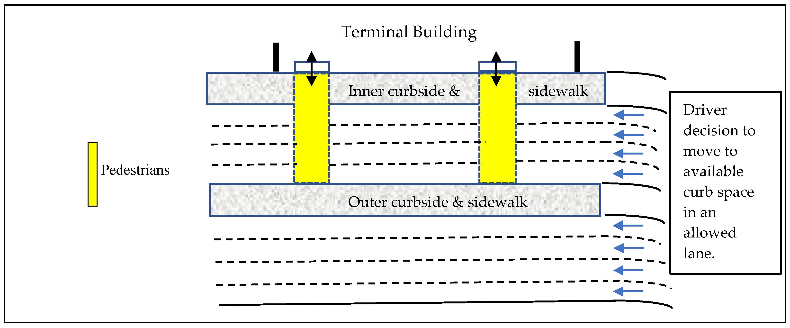
Figure 2.
Probability-based macrosimulation method.
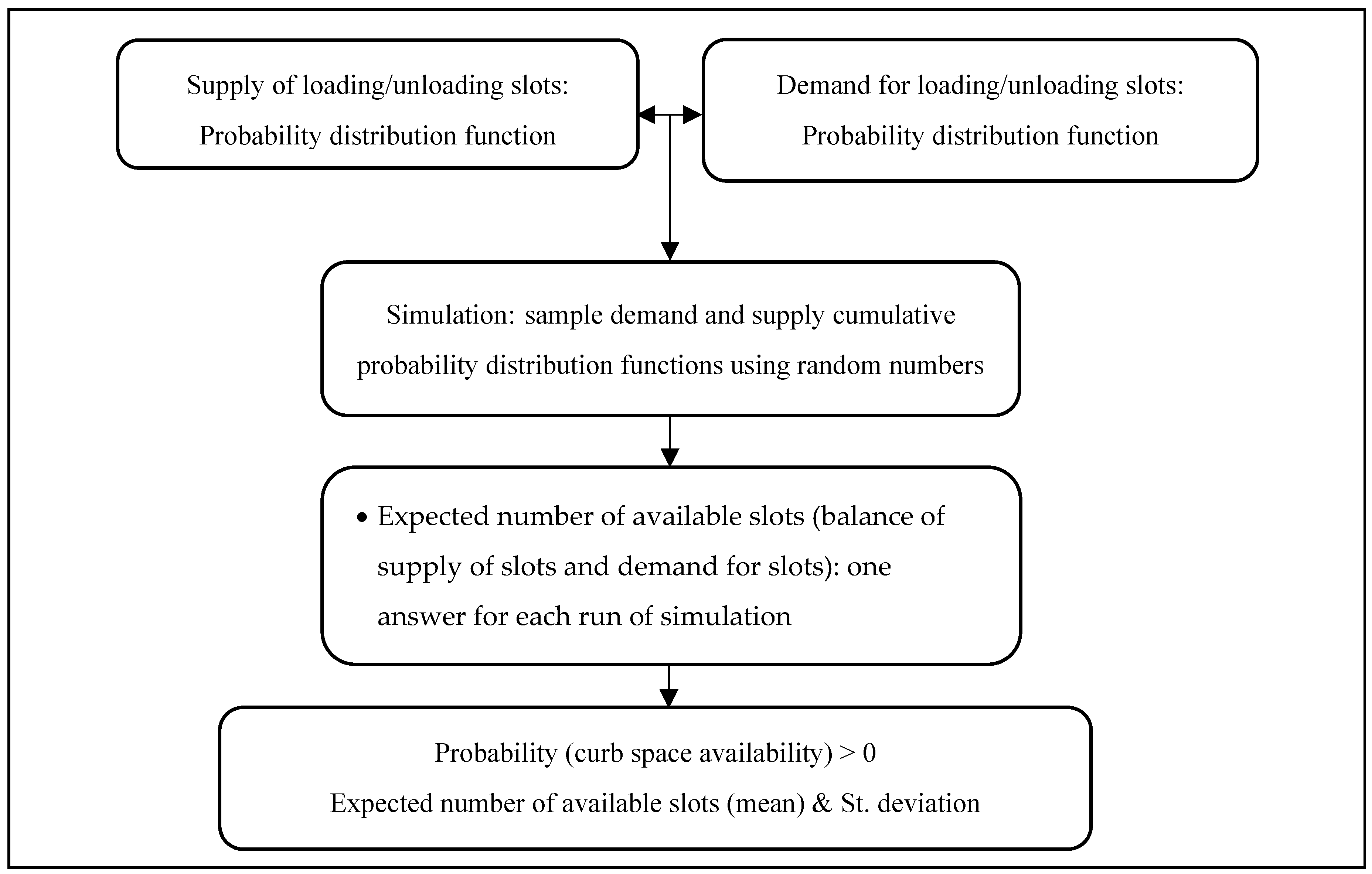
Figure 3.
Triangular Probability distribution function applied to demand and supply factors.
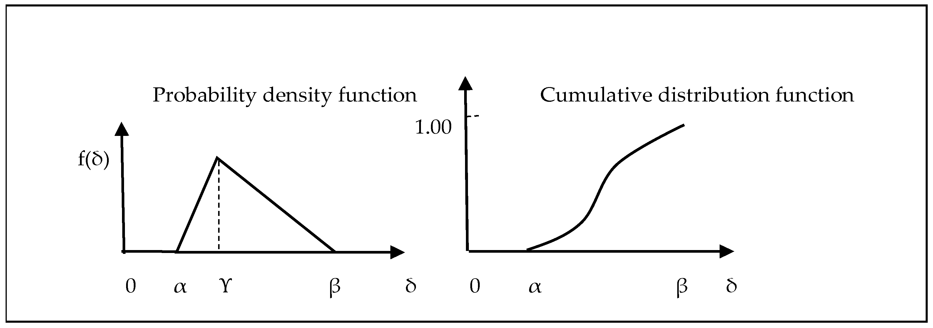
Figure 4.
Simulation of supply greater than demand (demand and supply vary from 0 to 40 slots).
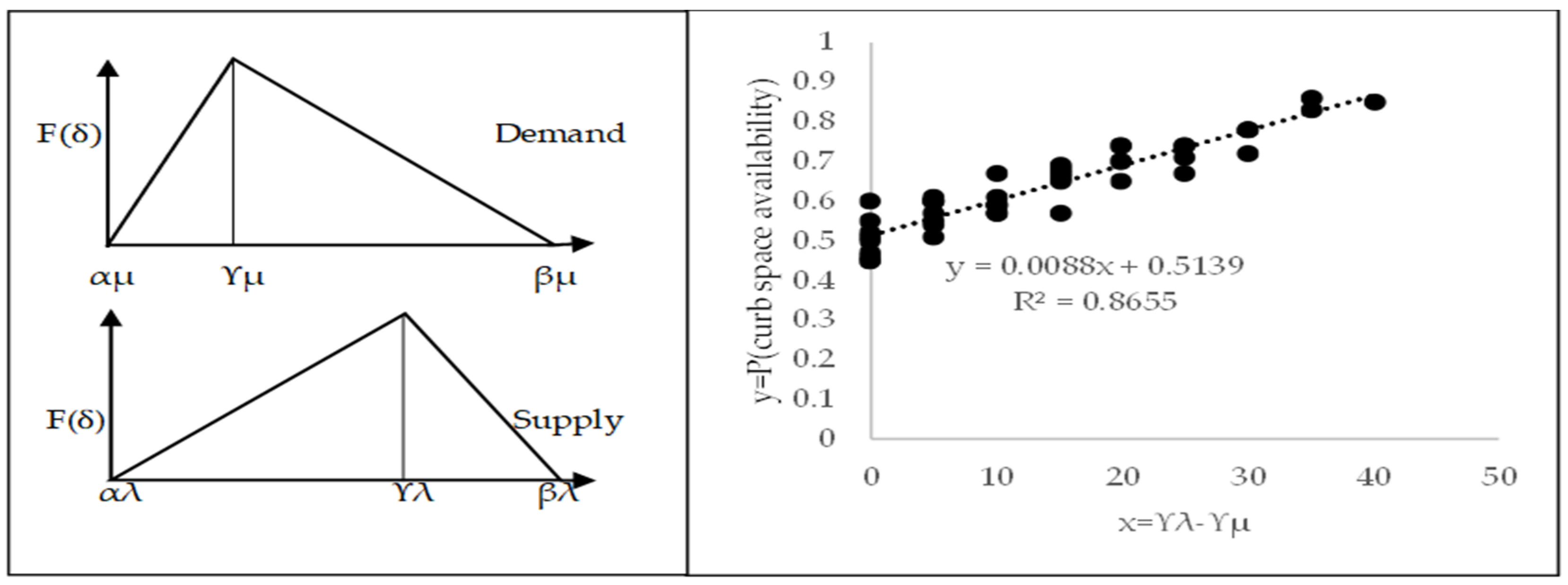
Figure 5.
Simulation of demand higher than supply (demand and supply vary from 0 to 40 slots).
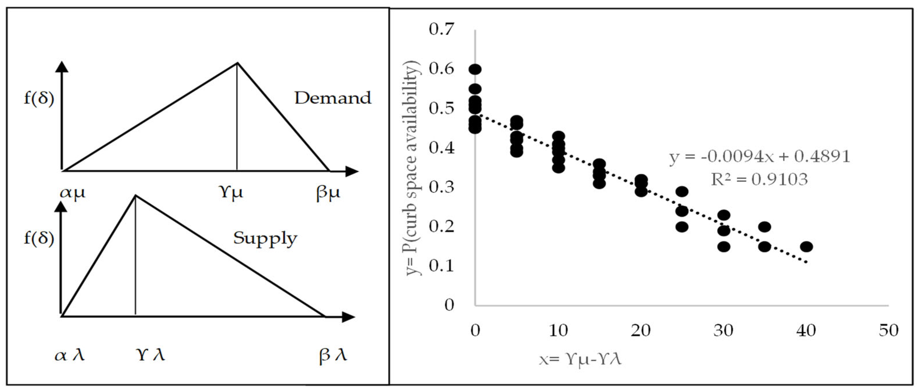
Figure 6.
Results for demand and supply equal to 140 slots each.
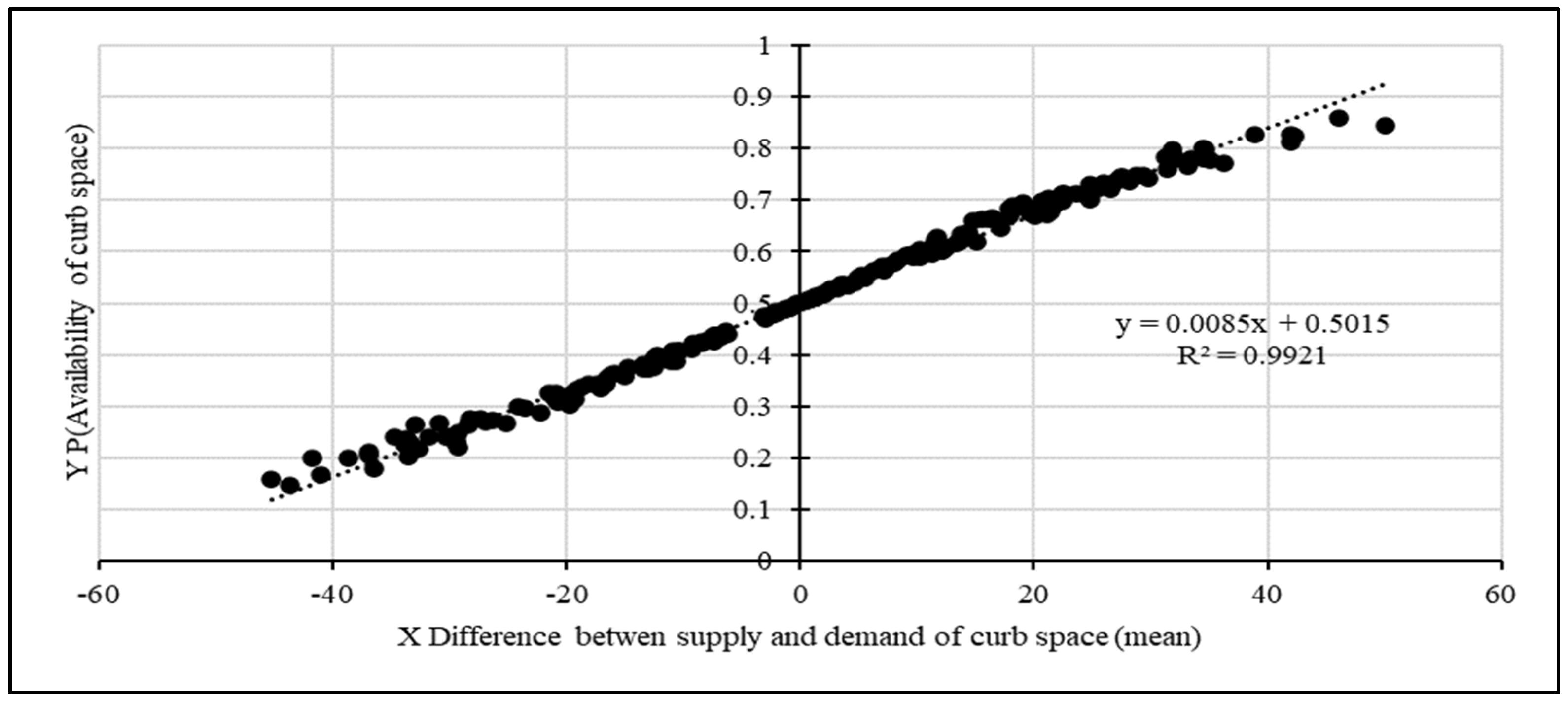
Figure 7.
Results of 40 supply time slots and 40 demand time slots.
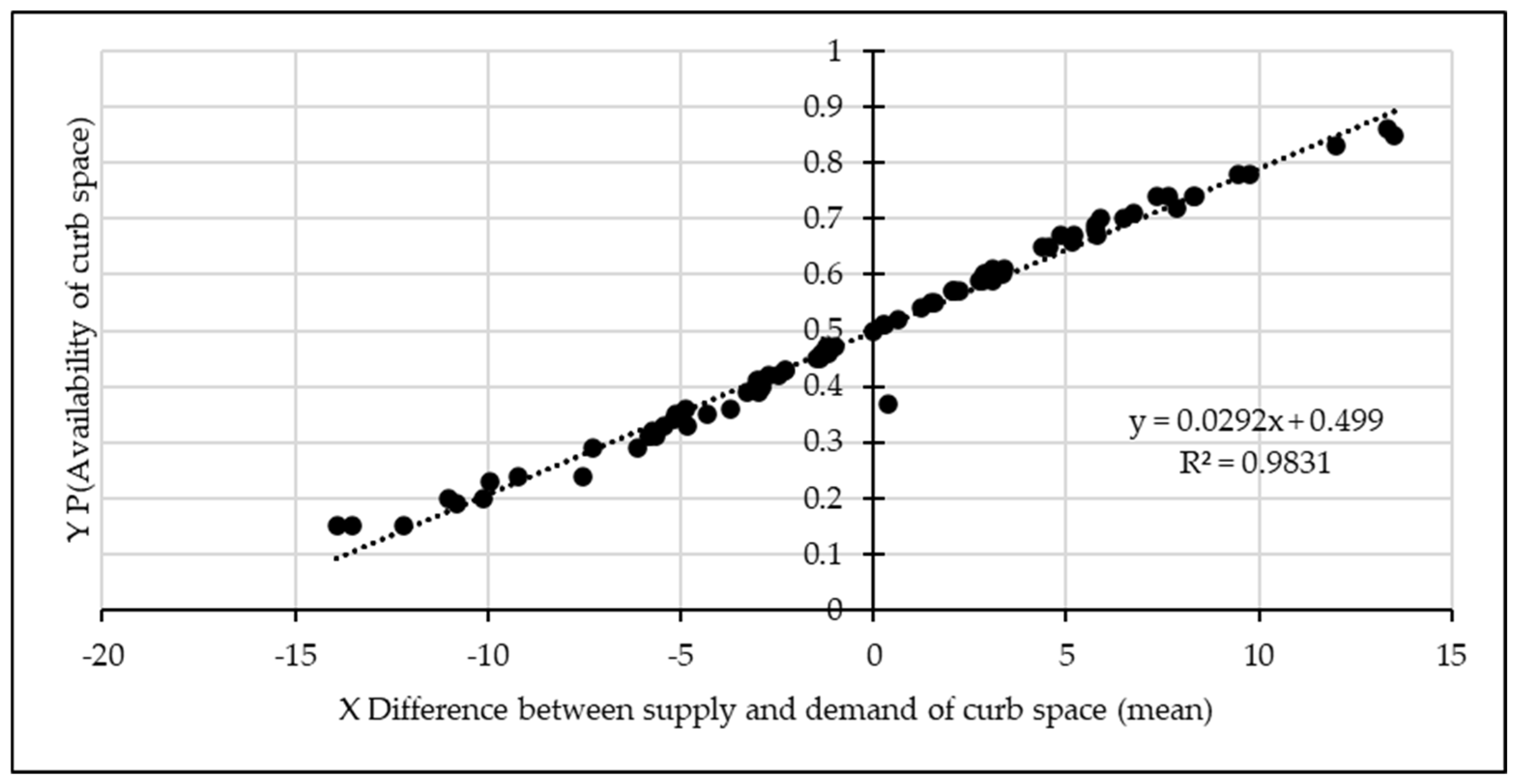
Figure 8.
Results for demand and supply equal to 140 slots each.
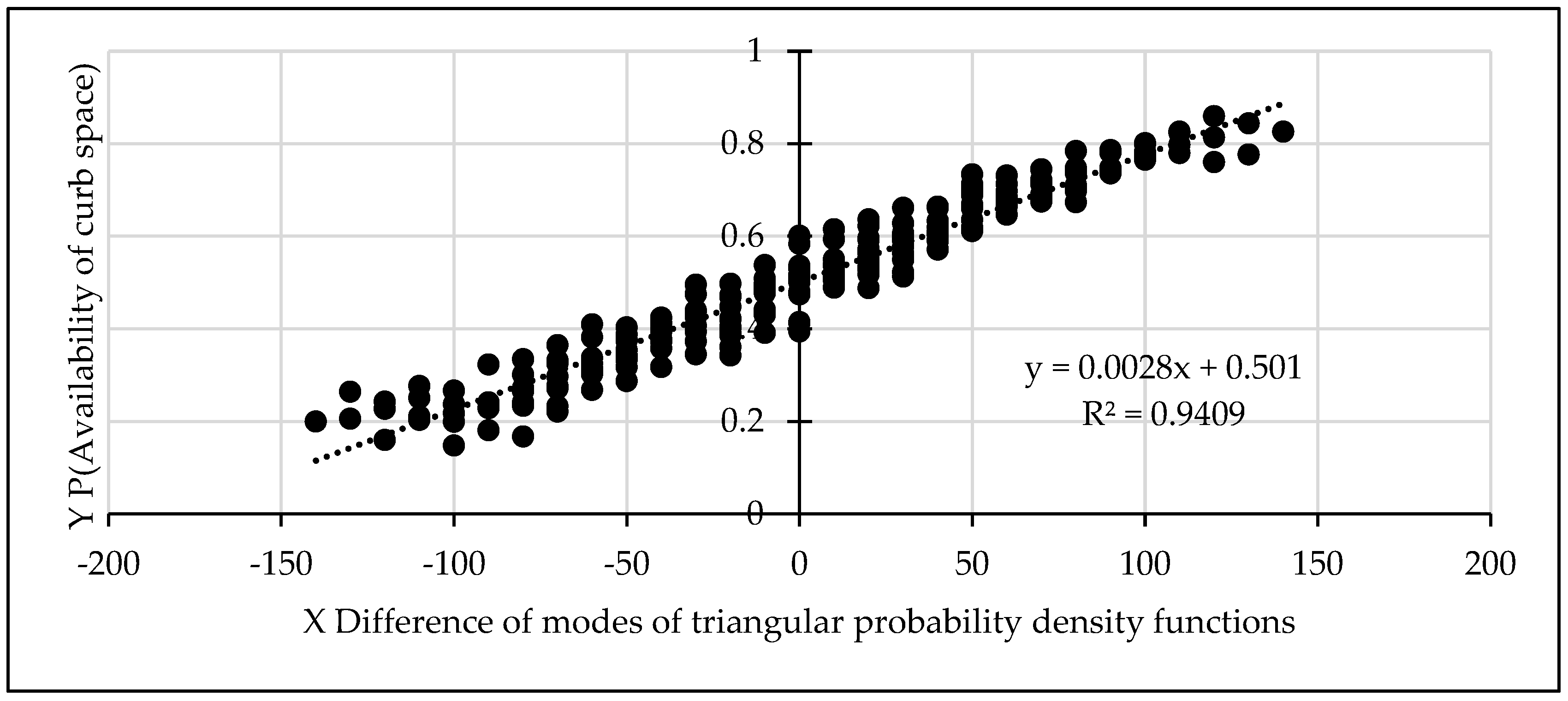
Figure 9.
Results for 140 slots demand and 280 slot capacity.
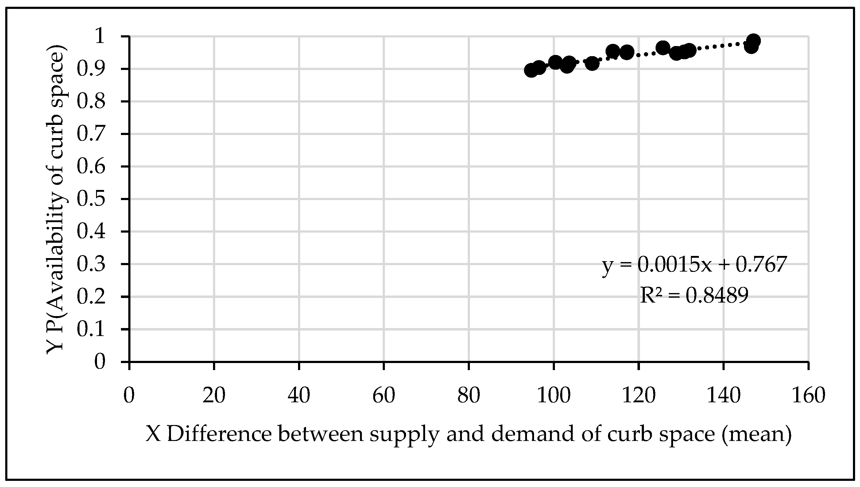
Figure 10.
Results of 280 supply time slots and 210 demand time slots.
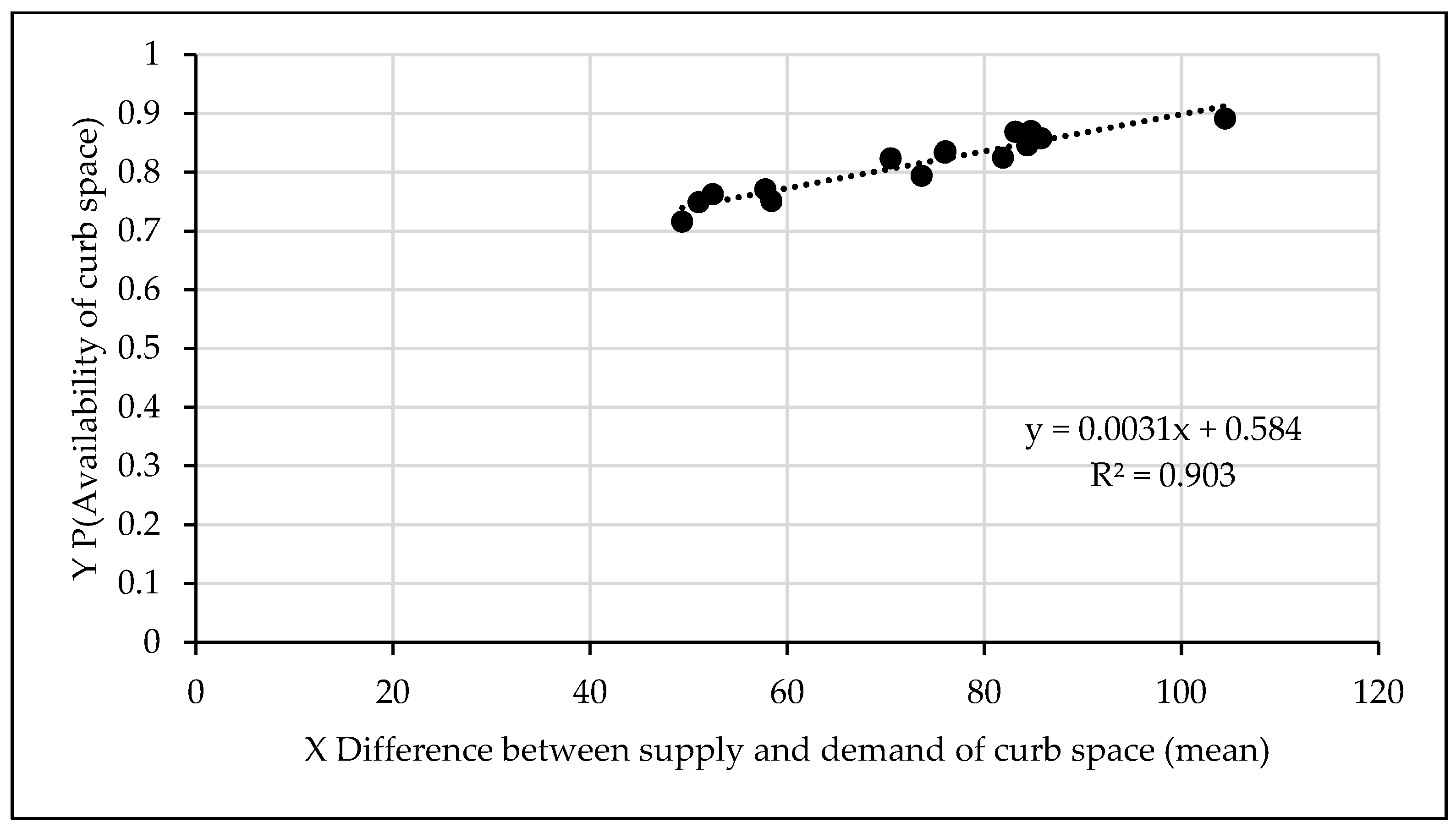
Figure 11.
Results of 280 supply time slots and 280 demand time slots. [NOTE: Probability of less than 0.5 results are not shown.].
Figure 11.
Results of 280 supply time slots and 280 demand time slots. [NOTE: Probability of less than 0.5 results are not shown.].
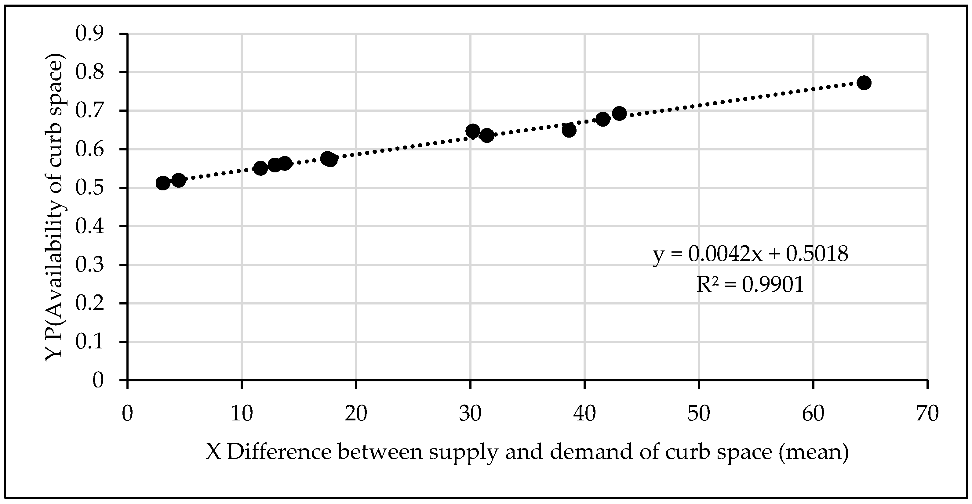

Table 1.
Comparison of candidate continuous probability distribution functions.
|
Uniform distribution Inputs: Supply of time slots: 0-40. Demand for time slots: 0-20 Results:
|
|
Triangular distribution Inputs: Supply of time slots: 0-40. Mode: 20. Demand for time slots: 0-20, Mode: 10 Results:
|
|
Normal distribution Inputs: Supply of time slots: Mean value 20 (midpoint of 0 to 40 slots), St. deviation 10 (assumed), Demand for time slots: Mean value 10 (midpoint of 0 to 20 slots), St. deviation 5 (assumed) Results:
|
Table 2.
Level of service concepts.
| Level- of- service (LOS) | Probability of (curb space availability when demanded) | Comments |
| A | 0.9 – 1.0 | Represents no delay condition; low demand periods. |
| B | 0.8-0.89 | Almost no delay; moderate demand periods. |
| C | 0.7-0.79 | Average demand periods: moderate delays can be expected. |
| D | 0.6-0.69 | Onset of peak demand condition and delays can be expected. |
| E | 0.5-0.59 | The LOS E reflects capacity level operations to accommodate peak demand condition. Due to demand surges, the LOS E can deteriorate to LOS F. |
| F | Below 0.5 | At LOS F, the operations at the curb part of the airport break down. Due to high delays, double and triple illegal parking may be attempted by some demand agents in the absence of traffic control. |
Table 3.
Delay index for 140 demand and supply time slots.
| Level of service (LOS) | Probability of the availability of a time slot | Expected mean available slots | Time slot unavailability index | Delay index (multiple of the time slot duration) |
| A | 1.00 0.90 |
58.65 46.88 |
1 – (58.65/58.65) = 0 1 – (46.88/58.65) = 0.20 |
0 0.20 |
| B | 0.89 0.80 |
45.71 35.12 |
1 – (45.71/58.65) = 0.22 1 – (35.21/58.65) = 0.40 |
0.22 0.40 |
| C | 0.79 0.70 |
33.94 23.32 |
1 – (33.94/58.65) = 0.42 1 – (23.32/58.65) = 0.60 |
0.42 0.60 |
| D | 0.69 0.60 |
22.18 11.59 |
1 – (22.18/58.65) = 0.62 1 – (11.59/58.65) = 0.80 |
0.62 0.80 |
| E | 0.59 0.50 |
10.41 0 |
1 – (10.41/58.65) = 0.82 1 – (0/58.65) = 1.00 |
0.82 1.00 |
Table 4.
Delay index for 40 demand and supply time slots.
| Level of service (LOS) | Probability of the availability of a time slot | Expected mean available slots | Slot unavailability index | Delay index (multiple of the time slot duration) |
| A | 1.00 0.90 |
17.16 13.73 |
1 – (17.16/17.16) = 0.00 1 – (13.73/17.16) = 0.20 |
0 0.20 |
| B | 0.89 0.80 |
13.39 13.31 |
1 – (13.39/17.16) = 0.22 1 – (13.31/17.16) = 0.40 |
0.22 0.40 |
| C | 0.79 0.70 |
9.97 6.88 |
1 – (9.97/17.16) = 0.42 1 – (6.88/17.16) = 0.60 |
0.42 0.60 |
| D | 0.69 0.60 |
6.54 3.46 |
1 – (6.54/17.16) = 0.62 1 – (3.46/17.16) = 0.80 |
0.62 0.80 |
| E | 0.59 0.50 |
3.12 0.03 |
1 – (3.12/17.16) = 0.82 1 – (0.03/17.16) = 1.00 |
0.82 1.00 |
Table 5.
Checks made on delay index.
| Level of service (LOS) | Probability of the availability of a time slot | Delay index for 140 time slot case
(multiple of a time slot) |
Delay index for 40 time slot case (multiple of a time slot) |
| A | 1.00 0.90 |
0.0 0.20 |
0.0 0.20 |
| B | 0.89 0.80 |
0.22 0.40 |
0.22 0.40 |
| C | 0.79 0.70 |
0.42 0.60 |
0.42 0.60 |
| D | 0.69 0.60 |
0.62 0.80 |
0.62 0.80 |
| E | 0.59 0.50 |
0.82 1.0 |
0.82 1.00 |
NOTE: For LOS F, the delay index will exceed 1.0.
Table 6.
Comparison of P(curb space availability) for different number of time slots.
| Demand versus supply condition | CASE 1: 7 curb spaces, 3 minutes time slots, study duration is 3 minutes | CASE 2: 7 curb spaces, 3 minutes time slots, study duration is one hour |
|
Most favourable condition Low demand, high supply Most unfavourable condition High demand, low supply |
Demand: α=0, β=7, ϒ=0 Supply: α=0, β=7, ϒ=7 P(curb space availability) =0.84 Demand: α=0, β=7, ϒ=7 Supply: α=0, β=7, ϒ=0 P(curb space availability) =0.18 |
Demand: α=0, β=140, ϒ=0 Supply: α=0, β=140, ϒ=140 P(curb space availability) = 0.83 Demand: α=0, β=140, Supply: α=0, β=140, ϒ=0 ϒ=140 P(curb space availability) =0.20 |
Table 7.
Comparison with delay estimates reported by other studies.
1. Level of service (LOS) |
2. Probability of curb use time slot availability |
3. Delay index
4. (multiple of a time slot)+
|
5. Delay (sec.)+
6.
7.
8.
|
9. Delay comparison (seconds) |
|||
10. Small hub airports* |
11. Smaller medium airports* |
12. Medium hub airports* |
13. BIA International Airport** |
||||
14. A
|
15. 1.00 - 0.90 |
16. 0.0 - 0.20 |
17. 0 - 36 |
18. 6 |
19. 12 |
20. 30 |
21. 14-20 |
22. B
|
23. 0.89 - 0.80 |
24. 0.22 - 0.40 |
25. 40 - 72 |
26. 20 |
27. 39 |
28. 98 |
29. 31-95 |
30. C
|
31. 0.79 - 0.70 |
32. 0.42 - 0.60 |
33. 76 - 108 |
34. 33 |
35. 66 |
36. 165 |
37. |
38. D
|
39. 0.69 - 0.60 |
40. 0.62 - 0.80 |
41. 112 -144 |
42. 47 |
43. 93 |
44. 233 |
45. |
46. E
|
47. 0.59 - 0.50 |
48. 0.82 - 1.0 |
49. 148 - 180 |
50. 60 |
51. 120 |
52. 300 |
53. |
54. F
|
55. < 0.50 |
56. >1.0 |
57. >180 |
58. >60 |
59. >120 |
60. >300 |
61. 316 |
Disclaimer/Publisher’s Note: The statements, opinions and data contained in all publications are solely those of the individual author(s) and contributor(s) and not of MDPI and/or the editor(s). MDPI and/or the editor(s) disclaim responsibility for any injury to people or property resulting from any ideas, methods, instructions or products referred to in the content. |
© 2025 by the authors. Licensee MDPI, Basel, Switzerland. This article is an open access article distributed under the terms and conditions of the Creative Commons Attribution (CC BY) license (http://creativecommons.org/licenses/by/4.0/).
Copyright: This open access article is published under a Creative Commons CC BY 4.0 license, which permit the free download, distribution, and reuse, provided that the author and preprint are cited in any reuse.


