Submitted:
13 January 2025
Posted:
14 January 2025
You are already at the latest version
Abstract
In the era of globalization and information technology, the aviation industry has experienced rapid growth. However, the increase in flight numbers has exacerbated environmental issues such as exhaust emissions and noise pollution, raising significant concerns across society. This paper aims to explore the current state of environmental pollution within the aviation industry and propose solutions to promote the development of green airports and effective pollution control measures. This study primarily employs literature analysis. Initially, a preliminary evaluation index system was established to represent various aspects of aviation pollution. The system was then refined and optimized using the entropy weight method. Subsequently, kernel density estimation and Moran index methods are applied to analyze the temporal and spatial trends of the evaluation indicators. An empirical study is conducted to investigate the degree of endogenous correlation and lag effects among the indices. The results show that: (1) Regional Neutrality in Pollution Indicators. The spatial autocorrelation test reveals a lack of significant spatial correlation among the studied aviation environmental pollution indicators, indicating that these variables maintain a degree of regional neutrality. (2) Impact of Cargo Throughput on Pollution. The PVAR model analysis highlights that cargo throughput has a significant self-impact on aviation environmental pollution, indicating that monitoring and managing cargo operations could be crucial in predicting and mitigating future pollution levels.
Keywords:
Green airport
; Entropy weight method
; Kernel density estimation
; Moran index
; PVAR model
1. Introduction
In the contemporary era of globalization and information technology, the aviation sector has become an integral component of modern society. Air transportation significantly bolsters international trade, tourism, and cultural exchange, while simultaneously playing a vital role in global economic integration [1]. Nonetheless, the rapid expansion of the aviation sector has resulted in prominent environmental concerns, capturing the attention of governments and the public internationally. Though the aviation industry has reaped significant economic benefits [2], its environmental footprint has become a matter of grave concern. The convenience and expediency offered by air transport have revolutionized global supply chains and logistics cycles by enabling swift transit of goods and people across continents and oceans [3]. However, this aviation-dependent economy introduces severe environmental challenges [4].
Studies suggest that the environmental impacts of aviation predominantly emerge in three areas: greenhouse gas emissions, noise pollution, and energy consumption [5]. Aircraft significantly contribute to greenhouse gas emissions, particularly carbon dioxide (CO2) and nitrogen oxides (NOx), directly affecting air quality and indirectly contributing to global climate change through the greenhouse effect and ozone layer depletion [6]. The International Civil Aviation Organization (ICAO) reports that the aviation industry is responsible for nearly 2% of global CO2 emissions annually, and this percentage is anticipated to rise in the future [7]. Besides gas emissions, noise pollution is another significant concern in the aviation sector [8]. Constant exposure to high-intensity noise can result in hearing loss, sleep disturbances, and cardiovascular diseases [9]. Despite technological advancements in aircraft design aimed at noise reduction, the increasing number of flights continues to aggravate the noise pollution issue [10].
Energy consumption in the aviation sector is another pressing concern, impacting not only aircraft operation but also airports and the wider aviation supply chain [11]. The considerable energy requirements of aviation have serious environmental consequences, pushing the industry to explore eco-friendly technologies and sustainable development [12]. Green airports, focusing on efficient energy use, effective waste management, noise control, and ecological protection, have emerged as a key solution to these challenges [13]. Innovations such as renewable energy usage, flight path optimization, and the construction of soundproof facilities can help to alleviate the negative environmental impacts of airport operations [14]. Airlines are also exploring low-carbon technologies, such as sustainable aviation fuels (SAF) and the development of electric and hybrid aircraft to reduce flight emissions [15].
International cooperation is pivotal in the environmental protection of the aviation industry [16]. Governments and international organizations are implementing stringent environmental standards and policies to guide the aviation sector towards a sustainable future [17]. However, most existing research tends to concentrate on individual aspects of environmental impact and suggests solutions accordingly [18]. This study builds upon previous research and critical data, utilizing methodologies such as Life Cycle Assessment (LCA) and Data Envelopment Analysis (DEA) [19] to quantify the environmental performance of airports. This study utilizes a preliminary evaluation index system based on existing literature [20], which is further refined and optimized through the entropy weight method. It also conducts temporal and spatial trend analyses using Kernel Density Estimation (KDE) and Moran’s I method [21]. The study investigates the relationships among indicators using data from four international airports. The results offer new insights into the complexity of aviation-related environmental pollution and establish a reliable basis for policy optimization, management improvement, and technological innovation in the aviation industry [22].
2. Materials and Methods
2.1. Evaluation Indicators and Data Collection
This study draws on recent research related to aviation emissions and pollution control, based on the "Guiding Principle for Accelerating Energy Conservation and Emission Reduction Efforts" and the widely recognized objective of fostering sustainable development within the aviation industry. To develop the evaluation indicator system, the study references several key documents, including the Green Airport Evaluation Guidelines issued by the Civil Aviation Administration of China (CAAC), the 14th Five-Year Plan for Green Aviation Development, and research conducted by Wei [23].The system was designed with a focus on scientific rigor, comprehensiveness, and the availability of data. The structure and details of the aviation environmental pollution assessment indicator system are presented in Table 1.
The panel data utilized in this study covers the period from 2013 to 2022 and includes information from four major airports: Shanghai Pudong International Airport and Hongqiao Airport in China, as well as Los Angeles International Airport and San Francisco International Airport in the United States. The primary sources of this data include official websites such as those of the National Bureau of Statistics of China, Huajing Intelligence, as well as the annual reports and corporate social responsibility (CSR) reports for the years 2013 to 2022 from Shanghai Airport Group, Los Angeles International Airport, and San Francisco International Airport. Additional data were obtained from Statista, the National Environmental Monitoring Center of China, the official website of the U.S. Census Bureau, and the California Climate Investments website. In cases where data was missing, interpolation techniques were applied to estimate the missing values. Furthermore, the variables for the four airports in the evaluation indicator system were averaged to ensure consistency in the analysis.
2.2. Entropy Weight Method for Key Indicator Selection
In this study, the entropy value method was used to select important indicators, incorporating the time variable in the process of determining the entropy values. The specific steps are as follows:
Step 1: Standardization of indicator data using the extreme value method is essential to ensure accurate and reliable results. This step helps in identifying and removing any outliers that may skew the data, allowing for a more consistent and meaningful analysis.
Where θ = 2013, 2014, …, 2022; i = 1, 2, 3, 4. represent the four airports: Pudong International Airport, Hongqiao Airport, Los Angeles International Airport, and San Francisco International Airport; and j = 1, 2, …, 8. represent the eight secondary evaluation indicators: flight movements, passenger throughput, cargo throughput, energy consumption, environmental protection investment in emissions reduction, aviation revenue, total assets, and operating costs. Therefore, Xθij represents the value of the j-th evaluation indicator for the i-th airport in the θ-th year. Xjmin and Xjmax are the minimum and maximum values of the j-th evaluation indicator, respectively.
Step 2: Non-negative transformation:
A constant M is added to reduce bias. Based on previous literature [24], M = 0.00001.
Step 3: Determination of characteristic proportions for each indicator:
Step 4: Calculation of entropy value for each indicator:
Where k > 0 is a constant and the entropy value must fall within the range of 0 ≤ ej ≤ 1. Therefore, we choose .
Step 5: Calculation of indicator weights:
Step 6: Calculation of comprehensive scores:
By applying the entropy value distribution to the aviation environmental pollution evaluation indicator system, we obtained the entropy value weights for the specific indicators, as shown in Table 2.
As shown in Table 2, four measurement indicators - flight movements, cargo throughput, energy consumption, and operating costs - are assigned relatively high weights, with values of 0.286, 0.2549, 0.2274, and 0.1359, respectively. In contrast, the weights for other indicators such as passenger throughput, environmental protection investment for emissions reduction, aviation revenue, and total assets are much lower, with values of 0.0412, 0.0018, 0.0116, and 0.0412, respectively. The entropy weight method is used to determine the relative importance of each indicator in the evaluation system. Based on this, the study eliminates indicators with weights below 0.1, which includes passenger throughput, environmental protection investment in emissions reduction, aviation revenue, and total assets. Consequently, for the subsequent empirical analysis, the study will focus on four key variables: flight movements (TAL), cargo throughput (CT), energy consumption (EC), and operating costs (OC).
This study incorporates both a time trend analysis and a spatial autocorrelation test of panel data to examine the evolution patterns, characteristics, and spatial structure of the variables. The aim is to identify underlying patterns and relationships within the data, providing a more robust basis for the subsequent Panel Vector Autoregression (PVAR) model, and to explore the dynamic interactions between the variables. Some of the original data used in the analysis is presented in Table 3. To ensure consistency in the dataset, especially considering the need for international unit conversions, the study standardizes the units for the key variables. Specifically, flight movements (TAL) are expressed as the number of flights, cargo throughput (CT) is converted into metric tons, energy consumption (EC) is standardized to the equivalent tons of coal needed to produce the same amount of heat, and operating costs (OC) are adjusted to U.S. dollars based on the current exchange rate. This standardization allows for a consistent and comparable analysis across the different airports and time periods.
2.3. Analysis of Time Change Trend of Aviation Environmental Pollution
Next, we analyze the spatio-temporal variation trend of the evaluation index series data using the kernel density estimation method and Moran index. We empirically tested the endogenous correlation and hysteresis effect of each index.
In this study, kernel density estimation method is used, and the formula is as follows:
Here, n represents the total number of indicators, with n = 4 in this case. xi represents the specific indicators selected, which include TAL, CT, EC, and OC. h is the bandwidth, and generally, the value of the bandwidth is determined by the size of n. The relationship between h and n is expressed as: where c is 1.05 times the standard deviation of the data sequence. K is the chosen kernel function, as determined by previous literature [25]. This study selects the Gaussian kernel function, which is expressed by the following formula:
In this study, the above kernel density estimation function is extended from one-dimensional to multidimensional, and the formula is as follows:
Here, d represents the dimension of x, with d = 3 in this case, corresponding to the time dimension, indicator dimension, and Kernel density dimension. K is the Kernel density function.
2.4. Dynamic Correlation Analysis Based on PVAR Model
After determining that aviation pollution does not exhibit regional clustering similarity and has a dispersed spatial distribution, we further analyzed the spatial dynamic relationships and interaction mechanisms of various variables. To this end, we employed a PVAR model to analyze the panel data of four representative airports from 2011 to 2022. The mathematical model is as follows:
Where i represents the four airports, t denotes the year, and p indicates the lag order, which is optimally selected based on sample stationarity and subsequent data processing. yit represents the column vector of endogenous variables, αij denotes the matrix to be estimated, γi is the fixed effects matrix, θt represents the time effects, and εit is the regression residual of the model.
3. Results
The observation period is from 2011 to 2022, as shown in Figure 1. From the perspective of spatial distribution, Figure 1(a) shows that the central value of flight movements gradually shifts to the right, reflecting the steady improvement in the global aviation industry. Additionally, the rapid evolution in this trend is likely associated with global economic growth and population increase. In contrast, the changes in Figure 1(b), (c), and (d) show less variation. Regarding distribution patterns, except for cargo throughput, the data for flight movements, energy consumption, and operating costs across the four airports show a sharp increase in concentration around 2020. This reflects the changes in aviation demand before and after the COVID-19 pandemic, indicating that the pandemic had a significant impact on the number of flight movements, energy consumption, and operating costs for civil aviation companies. From the perspective of the expansion of the main peak width of the Kernel density function, the actual differences among the four airports are gradually decreasing, indirectly reflecting the convergence of strategies adopted by international leading companies in response to the promotion of green aviation practices. In terms of distribution extension, cargo throughput indicates increasingly balanced spatial development, suggesting that the scale of cargo
operations across the companies remains at a world-class level. The right tails of the Kernel density function for energy consumption and operating costs have become flatter, indicating a gradual reduction in spatial disparities among airlines in their efforts toward environmental management in aviation.
We applied Moran I index to analyze the spatial correlation of the four key indicators for the sample airports in Figure 1. The results, as shown in Table 4, indicate that all Moran's I indices are negative, meaning that the spatial correlation analysis is not significant. This indicates that the data show little to no spatial correlation. In terms of aviation-related environmental pollution, this suggests that pollution is not concentrated in specific spatial areas. The negative spatial autocorrelation for airport operating costs and energy consumption may reflect regional differences in economic and policy environments, which could impact airport operational efficiency and energy consumption patterns, thus affecting their sustainable development strategies.
Before conducting PVAR modeling, it is important to ensure that the panel data is stationary to avoid spurious regression. This can impact the validity of the model estimation and subsequent impulse response analysis. Therefore, this study conducted stationarity tests on the panel data by region for variables such as the number of flight movements (TAL), cargo throughput (CT), energy consumption (EC), and operating costs (OC). This step is crucial for ensuring the reliability of the results. We utilized several common testing methods, such as the LLC test, IPS test, HT test, and PP-Fisher test, to examine the stationarity of the panel data. Generally, a variable is considered stationary if it passes two or more of these tests. Some variables in this study are still considered stationary, even though they did not pass all the tests, because they passed at least two tests. For variables identified as non-stationary, we took the logarithm and performed multiple-order differencing until they passed the stationarity tests. After differencing, TAL, CT, EC, and OC are respectively renamed as DTAL, DCT, DEC, and DOC. The results show that at confidence levels of 10%, 5%, and 1%, the variables are found to be significantly stationary and reject the null hypothesis of non-stationarity. The T-values, which represent the results, are displayed in Table 5.
Where *, **, and *** indicate significance at the 10%, 5%, and 1% confidence levels, respectively, the results show that all four variables passed the tests. Additionally, this study performed cointegration analysis using the Kao Test, Pedroni Test, and Westerlund Test on the basis of passing the unit root tests. This further integration check of the data that passed the unit root tests helps to determine whether each series is stationary, which is crucial for interpreting the stability of the constructed model.
To capture the underlying patterns and trends in the data more effectively, it is crucial to select an appropriate lag order. Determining the correct lag order is essential for enhancing the accuracy and stability of the model's predictions. Before proceeding with the Panel Vector Autoregression (PVAR) modeling, it is necessary to determine the optimal lag length. The methods commonly used for selecting the optimal lag order include the Akaike Information Criterion (AIC), Bayesian Information Criterion (BIC), and Hannan-Quinn Information Criterion (HQIC). In this study, we employ all three of these criteria-AIC, BIC, and HQIC-to determine the optimal lag order for the model, as presented in Table 6. The asterisk (*) indicates the optimal lag order according to the results from the BIC, AIC, and HQIC criteria. The model selection process involves identifying the lag order that minimizes these information criteria, ensuring the best-fitting model for the data.
Using the Generalized Method of Moments (GMM) estimation technique, we developed a Panel Vector Autoregression (PVAR) model with DTAL, DCT, DEC, and DOC as endogenous variables and applied GMM estimation to obtain the first-order regression results for the PVAR model. To address potential fixed effects in the panel data, we further transformed the data using the Helmert transformation. This transformation technique is applied to all subsequent data used in the analysis, as shown in the results presented in Table 7. The table reports the estimated coefficients
For each variable, with the symbols *, **, and *** indicating statistical significance at the 10%, 5%, and 1% confidence levels, respectively. The notation "L1."denotes that the data have undergone first-order regression, and "(h)" indicates that the Helmert transformation has been applied to the data.
After completing the previously described steps, we further tested the robustness and explanatory power of the constructed PVAR model by assessing its long-term stability. This was done by calculating the unit root eigenvalues, as shown in Figure 2. The results indicate that the values of all variables lie within the unit circle (with a radius of 1), which means that the unit roots of the variables are all less than 1. This confirms the stability of the PVAR model, suggesting that the fluctuations among the variables are stable and exhibit relatively smooth behavior over time.
To explore the causal relationships between the variables, this study conducts a Granger causality test, and the results are presented in Table 8. In this context, if the P-value exceeds the significance thresholds of 10%, 5%, or 1% (i.e., greater than 0.1, 0.05, or 0.01), it suggests that the null hypothesis cannot be rejected. This indicates that there is no statistically significant relationship between the explanatory variable and the dependent variable. As shown in Table 8, the results reveal that the other three variables do not significantly affect flight movements (TAL), which suggests that TAL operates relatively independently. This finding implies that the number of flight movements can be analyzed separately in studies focused on aviation environmental pollution, with minimal influence from the other related factors.
The results indicate that cargo throughput (CT) displays a certain level of endogenous correlation, with other variables exerting a significant influence on its interaction. The P-value is extremely close to 0, indicating that, apart from CT being a cause on its own, the other variables collectively serve as Granger causes for CT. Similarly, flight movements (TAL) are found to be a Granger cause for energy consumption (EC), indicating that airports' energy consumption is strongly dependent on the number of flight movements. Additionally, the other three variables also have a significant effect on EC, with a P-value of 0.012. This suggests that interactions between these variables have a notable impact on aviation environmental pollution.
Finally, for operating costs (OC), the null hypothesis can be significantly rejected in all cases, indicating that OC is strongly related to the other variables in the context of aviation environmental pollution. This implies that decisions regarding aviation pollution are closely tied to cost considerations, and effective environmental policies can often lead to higher economic benefits, as they influence cost structures within the industry.
This study examines the dynamic relationships between variables by analyzing the impact of a one standard deviation shock on the current and future values of the variables within the system. This approach provides an intuitive understanding of how random disturbances affect the endogenous variables in the PVAR model. Specifically, the impulse response results for each variable are obtained by simulating 200 iterations using the Monte Carlo method, with the shock period set to 10 periods, as illustrated in Figure 3. The horizontal axis represents the number of lags corresponding to the shock, while the vertical axis shows the response magnitude of each variable to the shock. The red line represents the impulse response function, while the green and blue lines provide a confidence interval for the responses over time. The green line indicates the range within two standard deviations for positive deviations, and the blue line indicates the range for negative deviations.
Based on the Granger causality analysis, we observed that not all variables exhibited mutual relationships. Therefore, our analysis of impulse response functions focuses on the variables that passed the test: DEC(h) to DCT(h), DTAL(h) to DEC(h), DTAL(h) to DOC(h), DCT(h) to DOC(h), and DEC(h) to DOC(h). These relationships underscore the intricate interactions between internal factors in aviation and environmental pollution. As depicted in Figure 3, when a one standard deviation shock is applied to energy consumption, the response of cargo throughput is initially negative. Around period 3, there is a slight positive response, but it gradually decreases and approaches zero over time. This suggests that any temporary positive reaction is minimal, and the overall negative feedback prevails. This indicates that energy consumption exerts a persistent negative effect on cargo throughput, emphasizing the need for airports to consider energy usage in managing cargo throughput, as it significantly contributes to aviation pollution. When a one standard deviation shock is applied to flight movements, the change in energy consumption is slightly positive and approaches zero. This suggests that flight movements have a limited impact on energy consumption, which becomes less significant over time. It implies that emissions from energy consumption are not the main contributors to pollution, possibly because of the role of electricity consumption by airport facilities and surrounding infrastructure, which reduces the importance of the positive feedback. The diminishing positive response suggests that airports have made efforts to manage carbon emissions, but there is still room for improvement in energy efficiency for infrastructure. When a one standard deviation shock is applied to flight movements, the response of operating costs is initially negative, then increases around period 1, followed by positive feedback in period 2, before gradually declining. This indicates that during the early operational phase, flight movements do not yield significant profits for airports. However, as operations continue, profits rise, primarily due to the high initial investment in manpower, resources, and equipment. After overcoming the transition period, short-term profits can be realized. Nevertheless, airports should consider environmental protection measures, as neglecting them may undermine the positive impact, leading to diminishing returns over time. The response variable in all cases is operating costs, and the patterns for cargo throughput, flight movements, and energy consumption are consistent. Therefore, the analysis follows the same reasoning. Furthermore, these three variables are endogenous factors in aviation environmental pollution. Therefore, airports should focus more on fundamental environmental factors when evaluating cost-benefit relationships.
4. Discussion
This study initially applies the Kernel density estimation method to investigate the temporal evolution trends of the reference data for four variables influencing aviation environmental pollution from 2011 to 2022, from a three-dimensional perspective. This method facilitates a more intuitive comprehension of the development direction and heterogeneity of the research subjects. The visual representation shows that, aside from the unusual disruptions caused by the pandemic in different regions, the historical trends of the indicators are mostly stable and increasing, with the regional differences gradually decreasing.
A subsequent spatial autocorrelation test is performed to determine the existence of regional variations in aviation environmental pollution indicators. The results indicate an almost uniformly negative Moran’s I index, signifying an absence of spatial correlation among the studied factors. This implies that the variables under study maintain regional neutrality in the context of aviation environmental pollution research.
Subsequently, a PVAR model is established. Through panel data analysis and the Granger causality test, it is revealed that flight movements exhibit a certain degree of autonomy in relation to other variables, providing a focused viewpoint for addressing aviation emission issues in environmental pollution analysis. The impulse response analysis indicates that cargo throughput exerts the most significant self-impact over the forecast period. Additionally, operating costs also show a significant impact. However, other variables do not demonstrate significant future impact correlations. Therefore, the issue of cargo throughput can be utilized to predict the future impacts of the current state of aviation environmental pollution.
Author Contributions
Conceptualization, S.D. and C.Z.; methodology, S.D.; software, S.D.; validation, S.D., L.Z. and J.Z.; formal analysis, S.D.; investigation, S.D.; resources, C.Z.; data curation, C.Z.; writing—original draft preparation, S.D., L.Z. and J.Z.; writing—review and editing, S.D.; visualization, S.D.; supervision, S.D.; project administration, S.D.; funding acquisition, S.D. All authors have read and agreed to the published version of the manuscript.
Funding
This research was funded by the SHANGHAI MUNICIPAL FOUNDATION FOR PHILOSOPHY AND SOCIAL SCIENCE (2024BJC002), and General project of 2024 Annual Planning project of Chinese Association of Business Statistics (2024STZA05).
Institutional Review Board Statement
This study does not involve research that raises ethical concerns related to human or animal subjects.
Data Availability Statement
In this paper, the panel data of Shanghai Pudong International Airport and Hongqiao International Airport in China, Los Angeles International Airport and San Francisco International Airport in the United States from 2013 to 2022 are selected for analysis. The data of the research sample are mainly from the official website of the National Bureau of Statistics, the China Economic Information Network, the 2013-2022 annual report and social responsibility report of Shanghai Airport (Group) Co., LTD., the 2013-2022 Annual report and social responsibility report of Los Angeles International Airport, the 2013-2022 annual report and social responsibility report of San Francisco International Airport, and the statista data website, the National Environmental Monitoring Station, the official website of the National Bureau of Statistics, and the official website of California Climate Investment.
Conflicts of Interest
The authors declare no conflicts of interest.
References
- Group, A.G.E. ICAO reiterates CO2 offset scheme in 2020[J]. Argus global emissions: greenhouse gas trading, policies and regulation, 2014, 13(12):13-12.
- Zhang, F.; Graham, D.J. Air transport and economic growth: a review of the impact mechanism and causal relationships. Transport Reviews, 2020, 40(4), 506-528. [CrossRef]
- Behnam, F.; Michael, G.H.B.; David, A.H.; Joseph, S. The Role of Green Logistics and Transportation in Sustainable Supply Chains[J]. Green Logistics and Transportation, 2015, 4: 1-12. [CrossRef]
- Syeda, A.H.; Misbah, N.; Nazish, R.; Inayatul, H. Exploring the existence of aviation Kuznets curve in the context of environmental pollution for OECD nations[J]. Environment, Development and Sustainability,2021, 23(10): 15266-15289. [CrossRef]
- Arthit, C.C.; Dhakal, S.; Chollacoop, N.; Phdungsilp, A. Greenhouse gas emissions trends and drivers insights from the domestic aviation in Thailand[J]. Heliyon, 2024, 10(2): e24206. [CrossRef]
- Paul, D.W. Increased Light, Moderate, and Severe Clear-Air Turbulence in Response to Climate Change[J]. Advances in Atmospheric Sciences, 2017, 34(5): 576-586. [CrossRef]
- Homola, D.; Boril, J.; Smrz, V.; Leuchter, J.; Blasch, E. Aviation Noise-Pollution Mitigation Through Redesign of Aircraft Departures [J]. Journal of Aircraft, 2019, 56(5): 1907-1919. [CrossRef]
- Osborne, R. In September 2020, the World Health Organization called for ‘equitable access to COVID-19 tools’ which included ‘the development, production and equitable access to COVID-19 tests, treatments and vaccines globally, while strengthening health systems. What evidence is there of inequity of access so far in this pandemic? What is the role of national governments and of the WHO in this? [J]. Medicine, Conflict and Survival, 2021, 37(3): 187-196. [CrossRef]
- Tooth, C.C.; Kaux, J. F.; Sébastien, L.G.; Hannouche, D.; Seil, R.; Leclerc, S. Concussion in sport: An ongoing challenge[J]. Journal de Traumatologie du Sport, 2024, 41(3): 195-196. [CrossRef]
- Rosario, P. Morphing wing flaps for large civil aircraft: Evolution of a smart technology across the Clean Sky program[J]. Acta aeronautica sinica, 2021, 34(7): 13-28. [CrossRef]
- VermaCA1, A.; Chhabra, M.; Giri, A. K. ICT diffusion, energy consumption, institutional quality, and environmental sustainability in 20 emerging economies during 2005-2019[J]. International Journal of Environmental Science and Technology, 2024, 21(4): 4445-4456. [CrossRef]
- Walter, L.F.; Artie, W.N.; Janová, A.S.; Pınar, G.; Chinmai, H.; Graeme, H.; Dennis, N.; Izabela, R. Global tourism, climate change and energy sustainability: assessing carbon reduction mitigating measures from the aviation industry[J]. Sustainability Science, 2023, 18(2): 983-996. [CrossRef]
- Cosgrove, C. Green initiatives for sustainable airport services [J]. Journal of Airport Management, 2018, 12(4): 350-358. [CrossRef]
- Valohery, C.R.; Ionut, D.M.; William, G.D.; Thomas, M.; Bãdicã, C.; Raft, R. Modelling aircraft noise map around an airport using machine learning[A]. 2024 International Conference on INnovations in Intelligent SysTems and Applications, INISTA, 2024.
- König, P; Müller, P; Höschler, K. Assessment of (hybrid)-electric drive-train architectures for future aircraft applications[J]. Journal of Physics: Conference Series, 2023, 2526: 012023. [CrossRef]
- Han, B.; Kong, W.K.; Yao, T.W.; Wang, Y. Beijing-tianjin-hebei Airport Group aircraft LTO air pollutant emission inventory [J]. Environmental Science, 2020, 41: 1143-1150. [CrossRef]
- Girija, P.; Smita, M.; Sanjay, K.N.; Girija, K.B.; Paromita, C. A Scientific Approach to the Occurrence, Isolation, and Characterization of Existing Microplastic Pollution in the Marine Environment-a Review[J]. Water, Air, & Soil Pollution, 2023, 234(7): 1-23. [CrossRef]
- WhittleCA1, J.W.; Callander, K.; Akure, M.; Kachwala, F.; Koh, S.C.L. A new high-level life cycle assessment framework for evaluating environmental performance: An aviation case study[J]. Journal of Cleaner Production, 2024, 471: 143440. [CrossRef]
- Gracia, S; Soundarabai, P.B.; Pethuru, R. Towards a Smarter Connected Society By Enhancing Internet Service Providers' Qos Metrics Using Data Envelopment Analysis[J]. ECS Transactions, 2022, 107(1): 225. [CrossRef]
- Justin, R.; David, B.; Laurie, A.G.; Russell, W.M.; David, W. A new GIS database documenting the prevalence of U.S. air service development incentives[J]. Journal of Air Transport Management, 2022, 98: 102148. [CrossRef]
- Han, F.; Sui, F.M. Effect of Global Moran's I and Space-time Permutation Scanning Method in Shanghai Metro Traffic Based on Ecological Transportation System [J]. Ekoloji Dergisi, 2019, 28(107): 4741-4749.
- Ahmed, E.; Matevz, O.; Ahmed, H.A.; Mahmoud, B. Does environmental knowledge and performance engender environmental behavior at airports? A moderated mediation effect[J]. Business Process Management Journal, 2024, 30(3): 671-698. [CrossRef]
- Wei, H. China's Rural Development in the 14th Five-Year Plan Period[J]. China Economist, 2022, 17(1): 2-11.
- Yin, L.; Yi, J.; Lin, Y.; Lin, D.; Wei, B.; Zheng, Y.; Peng, H. Evaluation of green mine construction level in Tibet based on entropy method and TOPSIS [J]. Resources Policy, 2024, 88: 104491. [CrossRef]
- Elen, A; Selçuk, B; Közkurt, C. An adaptive Gaussian kernel for support vector machine[J]. Arabian Journal for Science and Engineering, 2022, 47(8): 10579-10588. [CrossRef]
Figure 1.
The 3D distribution pattern of four important indicators that affect aviation pollution.
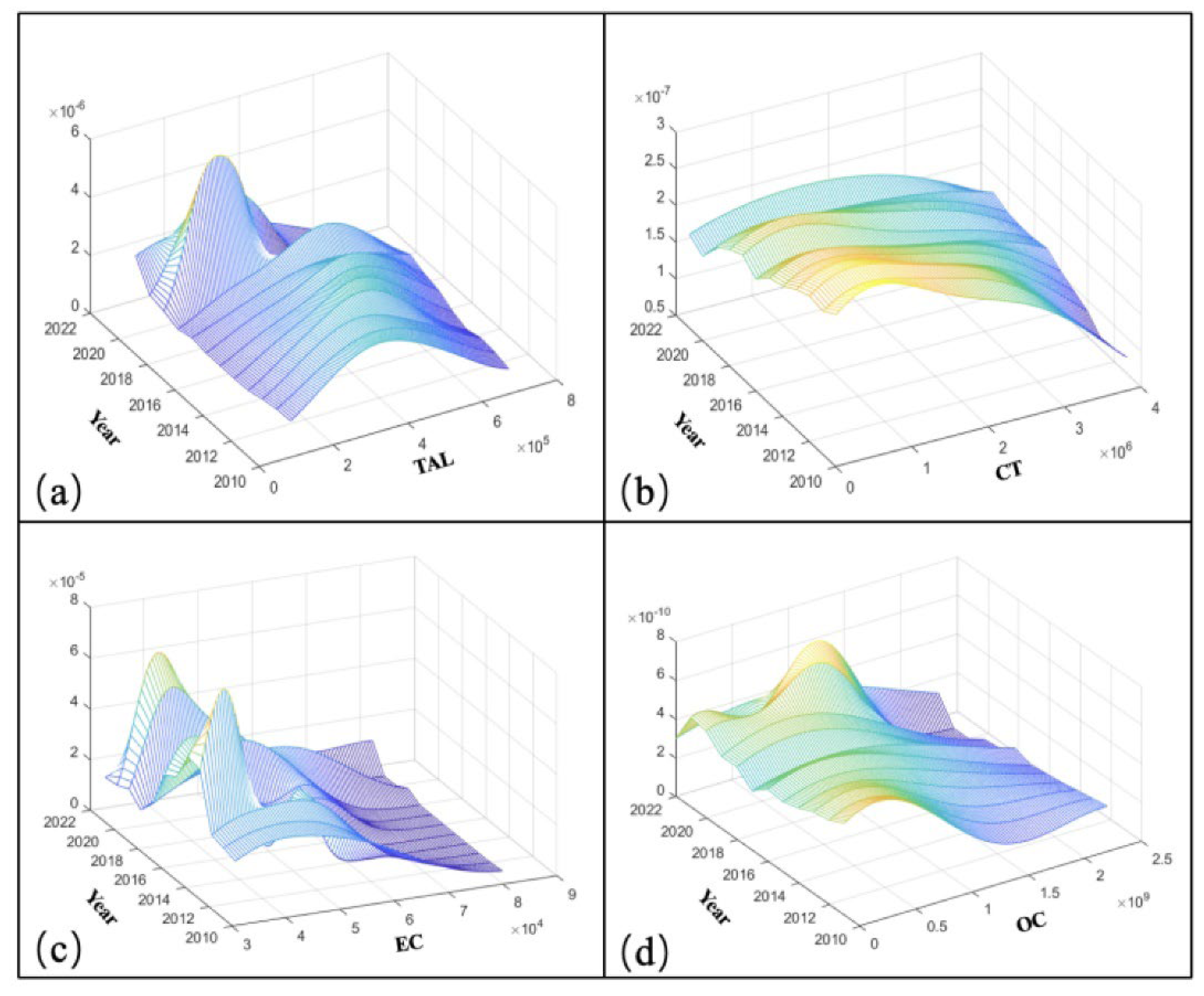
Figure 2.
Stability test result.
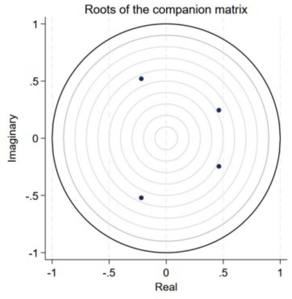
Figure 3.
Impulse response diagram between variables.
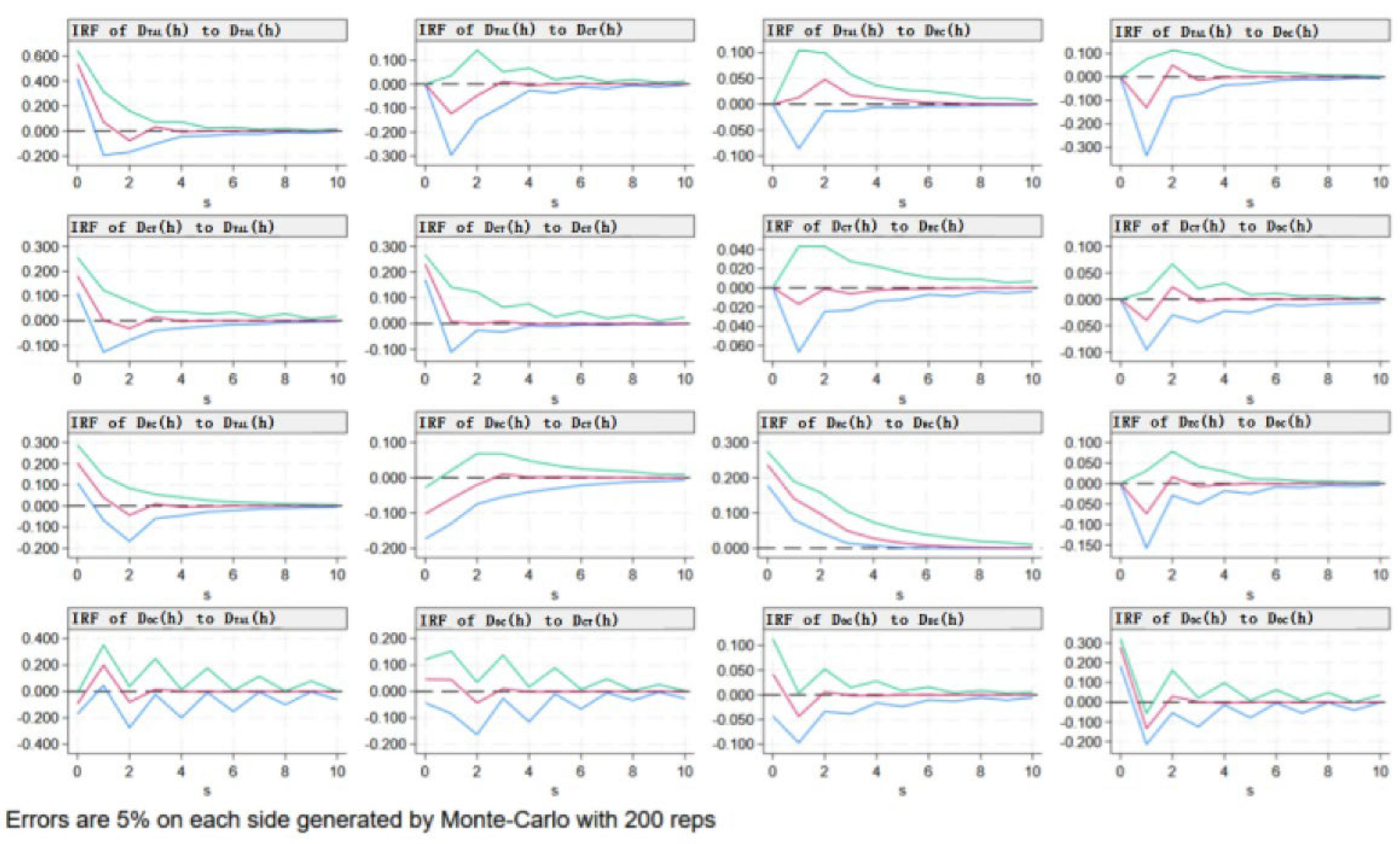

Table 1.
Aviation environmental pollution evaluation index.
| Primary indicators, | secondary indicators |
|---|---|
| Airport operation efficiency | Number of takeoffs and landings Passenger throughput Cargo throughput |
| Pollution prevention and environmental management | Energy consumption |
| Waste gas investment | |
| Economic efficiency and sustainable development | Aviation revenue |
| Total assets | |
| Operating cost |
Table 2.
Aviation environmental pollution evaluation index.
| level | Measure index | utility | weight |
|---|---|---|---|
| Airport operation efficiency | Number of takeoffs and landings | positive indicators | 28.60% |
| Passenger throughput | positive indicators | 4.12% | |
| Cargo throughput | positive indicators | 25.49% | |
| Pollution prevention and environmental management | Energy consumption | negative indicators | 22.74% |
| Waste gas investment | positive indicators | 0.18% | |
| Economic efficiency and sustainable development | Aviation revenue | positive indicators | 1.16% |
| Total assets | positive indicators | 4.12% | |
| Operating cost | negative indicators | 13.59% |
Table 3.
Some of the original data of four Aerodrome.
| Aerodrome | Year | TAL | CT | EC | OC |
|---|---|---|---|---|---|
| Pudong International Airport | 2011 | 344086 | 3085268 | 49737.28 | 43956366.78 |
| 2012 | 361720 | 2938157 | 50265.78 | 49372532.83 | |
| 2013 | 371190 | 2928527 | 51908.83 | 53440880.29 | |
| ... | ... | ... | ... | ... | |
| 2022 | 204378 | 3117215.59 | 82087.48 | 120773923.31 | |
| Hongqiao Airport | 2011 | 229846 | 454069 | 39734.93 | 2327961340.72 |
| 2012 | 234942 | 429814 | 37888.17 | 2210741181.40 | |
| 2013 | 243916 | 435116 | 39159.61 | 2066629650.83 | |
| ... | ... | ... | ... | ... | |
| 2022 | 122668 | 184538.10 | 37307.52 | 1552914839.79 | |
| Los Angeles International Airport | 2011 | 541852 | 1853658 | 59992.79 | 654523000 |
| 2012 | 559080 | 1963210 | 53976.41 | 714236000 | |
| 2013 | 578002 | 1926050 | 51564.83 | 733928000 | |
| ... | ... | ... | ... | ... | |
| 2022 | 475106 | 2754570 | 50720.63 | 1345660000 | |
| San Francisco International Airport | 2011 | 403564 | 340766 | 34039.04 | 494940000 |
| 2012 | 424566 | 337357 | 33175.26 | 543063000 | |
| 2013 | 421400 | 325782 | 33649.61 | 561458000 | |
| ... | ... | ... | ... | ... | |
| 2022 | 355006 | 491192 | 54202.55 | 809830000 |
Table 4.
Moran I test of 4 important indicators.
| Year | TAL | CT | EC | OC | ||||||||
| Moran I index | Normal statistics | p | Moran I index | Normal statistics | p | Moran I index | Normal statistics | p | Moran I index | Normal statistics | p | |
| 2011 | -0.294 | 0.135 | 0.446 | -0.497 | -0.456 | 0.324 | -0.461 | -0.392 | 0.348 | -0.647 | -1.171 | 0.121 |
| 2012 | -0.318 | 0.054 | 0.479 | -0.522 | -0.516 | 0.303 | -0.475 | -0.401 | 0.344 | -0.62 | -1.08 | 0.14 |
| 2013 | -0.325 | 0.028 | 0.489 | -0.508 | -0.48 | 0.315 | -0.423 | -0.259 | 0.398 | -0.603 | -1.022 | 0.153 |
| 2014 | -0.433 | -0.368 | 0.356 | -0.526 | -0.529 | 0.298 | -0.122 | 0.806 | 0.21 | -0.571 | -0.917 | 0.18 |
| 2015 | -0.562 | -0.858 | 0.195 | -0.557 | -0.608 | 0.272 | -0.277 | 0.203 | 0.419 | -0.532 | -0.776 | 0.219 |
| 2016 | -0.588 | -0.96 | 0.169 | -0.578 | -0.666 | 0.253 | -0.369 | -0.119 | 0.452 | -0.52 | -0.724 | 0.235 |
| 2017 | -0.607 | -1.035 | 0.15 | -0.629 | -0.808 | 0.209 | -0.537 | -0.702 | 0.241 | -0.444 | -0.449 | 0.327 |
| 2018 | -0.55 | -0.8 | 0.212 | -0.628 | -0.816 | 0.207 | -0.865 | -0.333 | 0.024 | -0.487 | -0.615 | 0.269 |
| 2019 | -0.645 | -1.168 | 0.121 | -0.648 | -0.866 | 0.193 | -0.822 | -1.584 | 0.057 | -0.446 | -0.458 | 0.323 |
| 2020 | -0.658 | -0.888 | 0.187 | -0.646 | -0.851 | 0.197 | 0.13 | 1.44 | 0.075 | -0.335 | -0.007 | 0.497 |
| 2021 | -0.618 | -0.841 | 0.2 | -0.662 | -0.891 | 0.187 | 0.094 | 1.424 | 0.077 | -0.268 | 0.276 | 0.391 |
| 2022 | -0.124 | 0.643 | 0.26 | -0.748 | -1.193 | 0.116 | -0.734 | -1.452 | 0.073 | -0.386 | -0.208 | 0.418 |
Table 5.
Unit root test for variables.
| Variables | LLC test | IPS test | HT test | ADF test | PP test | Conclusion |
|---|---|---|---|---|---|---|
| DTAL | -1.4591* | -2.0766** | -0.2093*** | 16.8174 | 16.3970** | Pass |
| DCT | -3.4367*** | -2.9732*** | -0.8850*** | 32.6348*** | 105.4283*** | Pass |
| DEC | -2.9028*** | -2.8062*** | -0.3735*** | 12.5723 | 49.9926*** | Pass |
| DOC | -3.3585*** | -2.9466*** | -0.7613*** | 19.7239*** | 96.2156*** | Pass |
Table 6.
The order of lag is determined.
| Lag | BIC | AIC | HQIC |
| 1 | 5.04704* | 3.69594* | 4.18446* |
| 2 | 5.89478 | 3.78342 | 4.52034 |
| 3 | 39.6651 | 36.7336 | 37.7053 |
| 4 | 46.5939 | 42.7876 | 43.9512 |
| 5 | 58.7348 | 54.0226 | 55.2728 |
Table 7.
GMM panel regression estimation results.
| Variables | DTAL(h) | DCT(h) | DEC(h) | DOC(h) |
|---|---|---|---|---|
| L1. DTAL(h) | 0.203 | -0.037 | -0.667 | 0.964*** |
| 0.896 | 0.461 | 0.516 | 0.314 | |
| L1. DCT(h) | -0.279 | 0.096 | 0.473 | -0.079 |
| 0.609 | 0.499 | 0.457 | 0.139 | |
| L1. DEC(h) | 0.155 | -0.061 | 0.802*** | -0.209*** |
| 0.237 | 0.175 | 0.180 | 0.081 | |
| L1. DOC(h) | -0.594 | -0.168 | -0.364 | -0.614*** |
| 0.597 | 0.159 | 0.304 | 0.108 |
Table 8.
Granger causality test results.
| Variables | Null hypothesis | chi2 | Degree of freedom | P |
|---|---|---|---|---|
| DTAL(h) | DCT(h) is not the null hypothesis of DTAL(h) | 0.05892 | 1 | 0.808 |
| DEC(h) is not the null hypothesis of DTAL(h) | 0.18785 | 1 | 0.665 | |
| DOC(h) is not the null hypothesis of DTAL(h) | 0.96202 | 1 | 0.327 | |
| None of the variables are null assumptions of DTAL(h) | 2.2908 | 3 | 0.514 | |
| DCT(h) | DTAL(h) is not the null hypothesis of DCT(h) | 0.00199 | 1 | 0.964 |
| DEC(h) is not the null hypothesis of DCT(h) | 4.2668 | 1 | 0.039 | |
| DOC(h) is not the null hypothesis of DCT(h) | 0.02698 | 1 | 0.870 | |
| None of the variables are null assumptions of DTC(h) | 22.954 | 3 | 0.000 | |
| DEC(h) | DTAL(h) is not the null hypothesis of DEC(h) | 3.5528 | 1 | 0.059 |
| DCT(h) is not the null hypothesis of DEC(h) | 0.00092 | 1 | 0.976 | |
| DOC(h) is not the null hypothesis of DEC(h) | 1.409 | 1 | 0.235 | |
| None of the variables are null assumptions of DEC(h) | 10.871 | 3 | 0.012 | |
| DOC(h) | DTAL(h) is not the null hypothesis of DOC(h) | 3.1018 | 1 | 0.078 |
| DCT(h) is not the null hypothesis of DOC(h) | 2.7063 | 1 | 0.100 | |
| DEC(h) is not the null hypothesis of DOC(h) | 6.4709 | 1 | 0.011 | |
| None of the variables are null assumptions of DOC(h) | 25.406 | 3 | 0.000 |
Disclaimer/Publisher’s Note: The statements, opinions and data contained in all publications are solely those of the individual author(s) and contributor(s) and not of MDPI and/or the editor(s). MDPI and/or the editor(s) disclaim responsibility for any injury to people or property resulting from any ideas, methods, instructions or products referred to in the content. |
© 2025 by the authors. Licensee MDPI, Basel, Switzerland. This article is an open access article distributed under the terms and conditions of the Creative Commons Attribution (CC BY) license (http://creativecommons.org/licenses/by/4.0/).
Copyright: This open access article is published under a Creative Commons CC BY 4.0 license, which permit the free download, distribution, and reuse, provided that the author and preprint are cited in any reuse.


