Submitted:
02 July 2025
Posted:
03 July 2025
You are already at the latest version
Abstract
Waterflooding is a key secondary recovery method in oil production, enhancing reservoir pressure and increasing extraction efficiency. Laboratory models, such as coreflood ex-periments, provide essential data on multiphase flow dynamics and reservoir properties, crucial for optimizing recovery techniques. Traditional analytical solutions for two-phase flow in porous media often neglect capillary pressure, limiting their accuracy in representing realistic scenarios. This study employs the Generalized Integral Transform Technique (GITT) to address nonlinear two-phase flow problems in heterogeneous porous media.The proposed solution considers the classical boundary condition, where maximum water saturation is assumed at the injection boundary. The Kirchhoff transformation is utilized to rewrite the governing equations, enabling a computationally more efficient GITT implementation. Results include the convergence analysis of the transformed and reconstructed solutions, verification against a numerical approximate solution, and an evaluation of low-order approximations, highlighting the method’s accuracy, computational efficiency, and potential applicability in inverse modeling scenarios.
Keywords:
secondary oil recovery
; coreflood experiment
; nonlinear convection
; relative permeability
; integral transforms
; GITT
1. Introduction
Secondary oil recovery plays a critical role in hydrocarbon extraction, aiming to enhance recovery beyond the capabilities of primary methods. After the initial production phase, which relies on the reservoir’s natural energy, secondary recovery techniques, such as water and-or gas injection, are employed to sustain or restore reservoir pressure. These methods not only improve extraction efficiency and extend the productive lifespan of oil fields but also contribute to reducing the environmental footprint of oil exploration and production while optimizing the economic viability of recovery operations [1]. In this context, for more than half a century, waterflooding has served as a reliable method of maintaining reservoir pressure and increasing oil production efficiency [2,3,4,5,6,7].
Given the importance of advanced oil recovery methods, laboratory scale models are critical for understanding not only the dynamics of multiphase flows in heterogeneous porous media, but also the properties of the reservoir rock, to properly plan water floods [8,9]. Coreflood experiments, for example, allow researchers to simulate and study flow behavior under controlled conditions, revealing important information about the mechanisms of oil displacement and the effectiveness of various recovery techniques [10]. These experiments provide important data for inverse problems, allowing the determination of intrinsic properties of the plug subjected to fluid flow, such as relative permeabilities [11,12,13,14,15,16,17].
A significant body of research has focused on numerically predicting water saturation dynamics and oil recovery in porous media, aiming to elucidate the complexities of multiphase flow in both multidimensional [18,19,20] and one-dimensional frameworks [21,22,23]. One-dimensional models, such as the Buckley-Leverett formulation and its variations [12,24,25,26], have been widely used to study two-phase flow in porous media. These simplified formulations effectively capture the fundamental physics of the problem while offering cost effective solutions, making them invaluable for understanding flow behavior in complex systems.
However, since these solutions neglect the influence of capillary pressure, they fail to accurately represent flows where this effect plays a significant role. Incorporating such terms introduces a strong nonlinear behavior into the problem. Nonlinear convective and diffusive effects and-or nonlinear source terms are frequently encountered in transport phenomena modeling, often resulting in nonlinear partial differential equations. These nonlinear formulations are generally unsolvable using traditional analytical methods [27,28,29,30]. Instead, they typically require approximate numerical approaches [31,32,33,34] or the application of mathematical techniques that involve dependent or independent variable transformations in specific formulations or approximate analytical solutions of limited scope [35,36,37,38].
As a result, numerical approaches have become the dominant choice for tackling nonlinear problems, supported by a range of effective algorithms and schemes. Nonetheless, there is a growing need to further improve the efficiency of computationally intensive processes, particularly in applications involving nonlinear formulations. These challenges are especially relevant in tasks such as inverse problems, optimization and uncertainty quantification, due to the usually required large number of runs of the direct problem solution, where the demand for scalability and computational feasibility continues to rise [39].
In response to the limitations of classical exact or approximate analytical solution techniques, the development of hybrid approaches that combine analytical and numerical techniques has gained significant traction. Among these, one particularly notable and mature methodology is the Generalized Integral Transform Technique (GITT). Initially introduced by Cotta and Ozisik [40] and subsequently extended through numerous contributions [41,42,43,44,45,46,47,48,49,50,51,52,53], GITT generalized the classical integral transform method originally developed for linear diffusion problems [27,28,29]. This meshless technique demonstrates the effective combination of the accuracy and computational efficiency of analytical solutions with the flexibility and generality of numerical solutions to tackle intricate engineering challenges, yielding error controlled solutions with moderate computational expense, allowing seamless incorporation with different tasks that demand extensive direct model evaluations.
The application of the Generalized Integral Transform Technique (GITT) to nonlinear problems is based on the idea that nonlinear partial differential equations can be reformulated to confine the nonlinear terms within the source terms, both in the governing equations and boundary conditions. This reformulation preserves linear characteristic coefficients, which define the associated eigenvalue problem. Through eigenfunction expansion and the integral transformation process, the reformulated nonlinear partial differential equation is transformed into a system of coupled, nonlinear, infinite transformed ordinary differential equations. This transformed ODEs system is then numerically solved to determine the transformed potentials, facilitating the analysis of complex nonlinear dynamics in the original problem.
Over the past three decades, following the introduction of GITT for nonlinear problems, this methodology has been progressively expanded to address a wide range of challenges. These extensions include applications to nonlinear models featuring variable physical properties, nonlinear source terms in both governing equations and boundary conditions, moving boundary problems, irregular domains, eigenvalue problems, nonlinear convection, diffusion or reaction-dissipation effects [41,42,43,45,46,47,48,49,51,54]. Recent applications of GITT that involve flow and transport in porous media can be cited such as pumping in confined, leaky, and unconfined aquifers [55], flow on fractured heterogeneous porous media [56], and flow in variably saturated porous media [57]. In reservoir engineering, GITT has been used in three-dimensional transient flow in heterogeneous reservoirs [58], two-dimensional energy balance for the transient temperature of sand faces in wells with mixed production [59], analysis of one-dimensional oil displacement by water injection in a core plug [60], and the two-dimensional convection-diffusion problem for tracer flow in a five-spot pattern [61,62].
Based on the discussion above and considering the potential of GITT and the importance of the addressed topic, this work presents a hybrid solution via GITT for immiscible two-phase flow in porous media with capillary pressure effects, which are highly relevant for reservoir studies. The formulation considers a two-phase flow in heterogeneous porous media, presenting linear and classical boundary conditions, which are independent of capillary pressure. In this demonstration, the effect of water injection at the rock’s boundary is expressed by a Dirichlet boundary condition, where the water saturation is at its maximum. The Kirchhoff transformation [28,37,63,64,65,66] is used to incorporate the nonlinearity of the diffusive operator originating from the capillary pressure into the transformed dependent variable to prepare the governing equation for the integral transformation via GITT. The test-case results here presented focus on the dynamics of the transformed and reconstructed solutions, highlighting convergence behavior, verification against an approximate numerical solution, and discusses the accuracy of low-order approximations.
2. Materials and Methods
2.1. Problem Formulation
Consider the two phase oil-water flow problem in a heterogeneous porous medium as shown in Eq. 1 [67]:
subject to the following boundary conditions (Eq. 2a and 2b) and initial condition (Eq. 2c):
In these, X represents the dimensionless spatial coordinate, such that the dimensional spatial coordinate x is defined as , with L being the length of the core, t the time, the water saturation such that , the spatial porosity distribution, the injected flow velocity, and the water fraction (Eq. 3) given as:
where and are the relative permeabilities of water and oil, respectively, and and are the dynamic viscosities of water and oil, respectively. The term , which is expressed as:
is the nonlinear diffusion coefficient due to capillary pressure, with being the oil mobility and the capillary pressure, and and the residual water and oil saturation, respectively.
2.2. Formal Solution
Let us apply the Kirchhoff transform [27,28,66] to the dependent variable , such that:
where is a reference water saturation. Then:
one obtains:
The transformed boundary and initial conditions are given by:
where:
A linear filter is used to homogenize the boundary condition at , according to the expression:
in which stands for the filtered potential, in the form:
The selected eigenvalue problem is based on the homogeneous version of the above filtered problem, such that:
which can be solved analytically. In the eigenvalue problem, the eigenfunctions are normalized using the following normalization integrals:
where i and j are integers, is the Kronecker delta function, and the normalized eigenfunctions are written as:
where is the normalization integral.
Based on the orthogonality relations, the transform-inverse pair is defined for the dependent variable:
If one applies the integral transform to Eq. 7b by integrating all terms in X from 0 to 1 after multiplying by the eigenfunction of the eigenvalue problem , one obtains:
where:
where the matrices and are nonlinear and thus time-dependent. Once the system presented on Eq. 16a is numerically solved for the transformed potentials along the time variable, the inverse formula (Eq. 15b) is recalled to reconstruct the potential U, which is finally inverted to provide the water saturation distribuition, , making use of the nonlinear relation (Eq. 5).
Depending on the functional form of the coefficient , the Kirchoff transformation, Eq. 5, shall require numerical integration. In this case, it is cost-effective to construct an interpolating function that provides a straightforward transformation within the domain of validity of the dependent variable . As for the inversion, again for some functional forms of , it may result in an analytical expression, otherwise a nonlinear algebraic equation roots algorithm needs to be employed. Again, an interpolating function construction shall be a cost-effective solution for the inversion process.
2.3. Test-Case
For the application of the solution presented in this work, a test case was selected based on the study by [68], specifically Case 3, in which . The capillary pressure is provided in the form of a data table (blue dots), which was interpolated using 5th order splines (black curve), as shown in Figure 1, for both the raw data and the interpolated curve within the domain of validity ( and ). The choice of 5th order splines led to the least numerical oscillations in the derivative estimates, but artificial smoothing can also be implemented at the cost of loosing the exact interpolation for in all the data points.
The extrapolation beyond the original data domain, i.e., the enforcement of constant values for at the extremes outside the valid range, is required because, during the numerical solution process, the potential function may assume values slightly outside the dependent variable domain, due to lower truncation orders relatively to the time value being considered. A similar approach was adopted by [21] and is discussed in the GitHub repository by [69]. If were to be estimated through a direct extrapolation of the fitted curve, unrealistic and physically inconsistent values might arise, resulting in amplification of the numerical error in the solution. Once the interpolation function for is constructed, the corresponding diffusion coefficient is computed according to Eq. 4.
Table 1 presents the input data used for the test case. The relative permeabilities are defined according to the Brooks & Corey relationship [70], given by:
where and represent the irreducible water and oil saturations, respectively, and and are real-valued exponents fitted to experimental observations. The maximum relative permeabilities of water and oil are denoted by and , respectively.
Figure 2 provides a graphical representation of the Kirchhoff transformation and its inversion for this test-case. It should be pointed out that for this particular behavior of the coefficient , in consequence of the behavior, while the transformation to the U domain is a fairly smooth function, the inversion to the domain is quite steep close to the domain limits, and . This requires a refinement of the interpolating points near these borders to ensure a proper accurate interpolation, otherwise a small deviation in the U value could cause an amplified deviation in the value and cause numerical weegles to appear in the representation of the water saturation field.
2.4. Shanks Transformation
The Shanks transformation [71,72] is a non-linear sequence-to-sequence acceleration method commonly used to improve the convergence of slowly convergent or even divergent series. Consider that each term of the eigenfuntion expansion represents one term in a given sequence. From this sequence, one can readily form the sequence of partial sums , up to the truncation order N. The first-order Shanks transform is defined as :
where represents an extrapolated estimate of the sequence’s limiting value. This transformation effectively removes the leading-order error term under the assumption that the sequence behaves locally as a linear combination of exponentials, thus providing an accelerated approximation to the series limit. Further convergence acceleration may be obtained by repeating the use of the Shanks transformation, applied to the new sequence , thus providing a second-, third-, and higher-order Shanks transforms. In this work, the Shanks transformation is employed to accelerate, when needed, or at least confirm the convergence of the computed GITT results.
3. Results
3.1. Convergence Analysis
This section presents the convergence analysis of the proposed integral transform solution. The truncation order in the eigenfunction expansion is initially fixed at , and the results are examined for different number of terms in the resulting series, in order to inspect the convergence behavior of the proposed expansion. All numerical integrations for the transformed system matrices and initial conditions vector are performed using Gaussian quadrature with points, ensuring that integration errors remain sufficiently low and controlled below the desired four digits accuracy in the final results throughout the analysis.
To accelerate and further verify the expansion convergence, the first-level Shanks transformation is applied to the partial sums of each sequence. The Shanks method provides an accelerated estimate of the series limit, which also serves as an additional consistency check for the computed values. Given the favorable convergence behavior already observed for moderate values of N, the contribution of the Shanks transformation in accelerating convergence is useful mostly at lower time values, yet confirms the robustness of the solution procedure.
The numerical results are summarized in Table 2, Table 3 and Table 4, for three distinct time instants (). In all cases, the solution is evaluated at five representative spatial positions (). A clear trend of convergence is observed as N increases, with full convergence to four significant digits at the highest value of N (± 1 in the last digit given), as confirmed by the Shanks transformation.
To complement the convergence study, a relative error analysis is conducted to quantify the accuracy of the truncated eigenfunction expansions. The objective is to assess how the partial sum of N terms compares to a reference solution obtained with terms. The relative residue estimate is defined as:
The results presented on Figure 3, Figure 4 and Figure 5, for five different dimensionless positions and three different times, demonstrate that even for relatively low truncation levels, such as , the relative residue remains below 1% at all relevant spatial and temporal positions. This highlights the efficiency of the proposed methodology in capturing the dominant dynamics of the system with a reduced computational cost.
The convergence tables presented so far refer to the values of computed at selected spatial positions and time instants. However, from a physical point of view, one needs to analyze the behavior of the water saturation , as this variable directly represents the fluid distribution within the porous medium. For completeness, we therefore provide below the corresponding convergence tables for , evaluated at the same dimensionless spatial positions and time instants used previously for .
These results are obtained by post-processing the values of through a numerical interpolation of the inverse Kirchhoff transform, but were also critically compared with the direct inversion through the nonlinear algebraic equation solver, without making use of the interpolated curve, and no difference has been observed with respect to the results shown below.

Table 5.
Convergence of for s and N up to 12.
| N | |||||
|---|---|---|---|---|---|
| 2 | 0.5608 | 0.4669 | 0.4043 | 0.3421 | 0.2 |
| 4 | 0.5578 | 0.4665 | 0.4056 | 0.3414 | 0.2 |
| 6 | 0.5579 | 0.4665 | 0.4056 | 0.3413 | 0.2 |
| 8 | 0.5584 | 0.4660 | 0.4055 | 0.3431 | 0.2 |
| 10 | 0.5586 | 0.4662 | 0.4056 | 0.3426 | 0.2 |
| 12 | 0.5586 | 0.4662 | 0.4055 | 0.3424 | 0.2 |
| Shanks | 0.5586 | 0.4662 | 0.4055 | 0.3424 | 0.2 |
Table 6.
Convergence of for s and N up to 12.
| N | |||||
|---|---|---|---|---|---|
| 2 | 0.5888 | 0.5096 | 0.4670 | 0.4405 | 0.4271 |
| 4 | 0.5876 | 0.5092 | 0.4674 | 0.4407 | 0.4269 |
| 6 | 0.5874 | 0.5093 | 0.4673 | 0.4408 | 0.4269 |
| 8 | 0.5873 | 0.5092 | 0.4673 | 0.4408 | 0.4269 |
| 10 | 0.5873 | 0.5092 | 0.4673 | 0.4408 | 0.4269 |
| 12 | 0.5873 | 0.5092 | 0.4673 | 0.4408 | 0.4269 |
| Shanks | 0.5873 | 0.5092 | 0.4673 | 0.4408 | 0.4269 |
Table 7.
Convergence of for s and N up to 12.
| N | |||||
|---|---|---|---|---|---|
| 2 | 0.6318 | 0.5687 | 0.5380 | 0.5213 | 0.5139 |
| 4 | 0.6304 | 0.5683 | 0.5384 | 0.5215 | 0.5137 |
| 6 | 0.6302 | 0.5684 | 0.5383 | 0.5215 | 0.5137 |
| 8 | 0.6301 | 0.5684 | 0.5384 | 0.5215 | 0.5137 |
| 10 | 0.6301 | 0.5684 | 0.5384 | 0.5215 | 0.5137 |
| 12 | 0.6301 | 0.5684 | 0.5384 | 0.5215 | 0.5137 |
| Shanks | 0.6301 | 0.5684 | 0.5384 | 0.5215 | 0.5137 |
In all examined time instants, the values of exhibit a clear convergence trend as N increases. Convergence to three significant digits can be observed for truncation orders as low as even at the lowest value of time. The application of the Shanks transformation further confirms this observation.
3.2. Verification Analysis
Figure 6 illustrates the spatial evolution of at selected time instants, namely s. These time points were chosen to encompass both the initial transient regime and the post-breakthrough phase of the saturation front. The results show that the solution maintains a smooth and well-behaved structure throughout the spatial domain for all times considered. Only for the lowest time value () it can be noticed, after careful inspection, that the transition region after the saturation front might require a few more terms in the expansion.
Figure 7 presents a verification analysis performed by comparing the proposed solution with a numerical solution obtained using NDSolve, Mathematica’s built-in PDE solver. Due to numerical instabilities encountered when solving the full nonlinear PDE directly, it was necessary to benefit from the Kirchoff transformation as well. Even then, NDSolve was not able to handle the nonlinearity due to the capillary pressure, and it was necessary to introduce a simplification in the diffusive term, the nonlinear coefficient was evaluated using the known solution obtained by the present method itself. This semi-coupled strategy yielded an approximate numerical result that still serves as a meaningful result for verification purposes.
The comparison revealed a good agreement between the proposed solution and the approximate numerical solution with NDSolve, particularly at early and intermediate times. As expected, a gradual loss of accuracy is observed at larger times, which is attributable to the approximation introduced and propagated in the numerical solution by NDSolve. in the numerical model. Nevertheless, the level of agreement remains sufficient to verify the GITT-based solution.
3.3. Low Order Truncation Solution
In the context of inverse problems and other computationally intensive tasks that require multiple evaluations of the direct problem solution, the use of low-order truncation expansions is particularly attractive, in combination with the Approximation Error Model (AEM) methodology [73,74], as it significantly reduces computational cost, without compromising the overall precision in the estimations. In this section, we investigate the behavior of the solution when the number of terms is limited to .
It is important to emphasize that when the eigenfunction expansion is restricted to low order truncation such as , it is inherently assumed that all transformed components for are identically zero. On the other hand, one may also extract the truncated expansions for instance up to from a computed solution with , in which case the contributions from higher-order modes ( to 12) are present in the solution space but excluded from the partial sum. As such, these two approaches yield different results, and this distinction becomes relevant when evaluating the implications of model truncation in inverse analyses, combined with the AEM approach.
To illustrate the behavior of a low truncation expansion, we compare three sets of results for three representative time instants: (i) direct computations with increasing N up to 6 (with ); (ii) the Shanks-transformed value at ; and (iii) the truncated expansion at extracted from the truncated expansion. Table 8, Table 9, and Table 10 report the values of for each time value at five spatial positions.
The comparison reveals that the direct solutions are remarkably close to the Shanks accelerated estimates, which confirms that the expansion with is essentially converged. Nevertheless, when comparing with the truncated sum at of the expansion with terms, the deviations are more noticeable, though always below 2.5% from these tables, but for accurate estimates should be accounted for by the approximation error model when implementing the inverse problem analysis.
This observation supports the use of low-order truncations, such as in the present example, as efficient and reliable. Therefore, the results suggest that a truncated solution with can serve as a robust surrogate for the full model in inverse formulations, enabling efficient parameter estimation while preserving the essential physical features of the system.
In sequence, we analyze the influence of the numerical integration accuracy on the final solution, by varying the number of Gaussian quadrature points used in the evaluation of the transformed terms . Although all previous results were computed with to eliminate integration-induced errors from the convergence study, it is relevant to assess the effect of reducing , particularly in the context of inverse problems, when computational savings are always at a premium.
Table 11, Table 12 and Table 13 present the values of obtained for and , for the same spatial positions and time instants previously analyzed. The Shanks transformation results computed with are included for comparison.
The results indicate that the solution converges rapidly with respect to , and that already provides values very close to the reference with and . At , the results are already converged to ± 1 in the fourth significant digit, indicating that the numerical integration error becomes irrelevant to within the desired accuracy in the final results.
For applications that require a large number of the direct problem evaluations, such as most parameter estimation in inverse formulations, this reduction in integration cost can lead to substantial performance gains.
4. Discussion
The results presented in the previous sections confirm the robustness, efficiency, and accuracy of the proposed solution for immiscible two-phase flow in porous media based on the Generalized Integral Transform Technique (GITT). The convergence analysis demonstrated that a relatively low number of terms in the truncated eigenfunction expansion () suffices to achieve converged and precise solutions for both the Kirchhoff-transformed variable and the physically meaningful saturation field . The use of the Kirchhoff transform is handy in partially incorporating the nonlinearity due to the capillary pressure effect into the dependent variable and thus reducing the stiffness in the transformed ODE system numerical solution. Besides, as previously observed in [39], it offers an inherent convergence acceleration bonus, as more information on the original problem nonlinear diffusive operator is aggregated to the dependent variable. These findings are particularly relevant in the context of inverse problems, where computational tractability is a key requirement.
The agreement between the GITT-based solution and the approximate numerical one provided by NDSolve provides verification of the implemented simulation. Despite the simplification that had to be adopted in the numerical simulation, where the nonlinear coefficient in the diffusive term was evaluated from the hybrid GITT solution itself, the match remains consistently good across the spatial and temporal domains. Minor discrepancies at longer times are attributed to the error propagation in the approximate numerical procedure rather than flaws in the proposed methodology.
From a computational standpoint, the analysis of numerical integration effects revealed that Gaussian quadrature with as few as points already yields negligible error to the final water saturation results at the lower truncation order or , indicating that the method is not only accurate but also computationally efficient. This supports the potential use of the present formulation in repeated simulations, such as those encountered in parameter estimation or uncertainty quantification tasks.
Moreover, the truncated low-order reduced model was shown to retain the essential features of the full solution while offering significant reductions in computational cost. The comparison between the truncated models and the higher-order solution confirms that even the low order truncated expansion preserved accuracy always below 2.5%, which is certainly acceptable for combining with the AEM for inverse problem analysis. This suggests that the approach can serve as a reliable reduced-order model in inverse formulations, where repeated forward evaluations are required.
In the broader context of modeling nonlinear flow in porous media, the present methodology offers a valuable alternative to conventional numerical solvers. It combines the interpretability and structure of analytical approaches with the flexibility of numerical integration, enabling hybrid strategies that are particularly well-suited for data assimilation, control, inverse problems, and optimization scenarios.
Future research may extend the current formulation to include more complex boundary conditions and multi-dimensional geometries. The flexibility of the integral transform approach also allows for its integration with Bayesian inference frameworks, further expanding its applicability in modern reservoir characterization workflows.
Funding
This research was carried out in association with the ongoing R&D project registered as ANP nº 24.551, “Avaliação de Metodologias para Interpretação de Curvas de Permeabilidade Relativa em meios porosos heterogêneos " (UFRJ/Petrobras Brasil/ANP), sponsored by Petróleo Brasileiro S/A under the ANP R&D levy as “Compromisso de Investimentos com Pesquisa e Desenvolvimento” and it was financially supported by the Human Resources Program of the National Agency of Petroleum, Natural Gas, and Biofuels – PRH-ANP, supported with resources from the investment of qualified oil companies under the R&D Clause of ANP Resolution No. 50/2015; and, in part, by the São Paulo Research Foundation (FAPESP), Brasil. Process Number 2024/11459-9.
Acknowledgments
GMS and RMC would like acknowledge the partial financial support of CNPq, FAPERJ, and CAPES, all of them research sponsoring agencies in Brazil.
Conflicts of Interest
The authors declare no conflicts of interest. The funders had no role in the design of the study; in the collection, analyses, or interpretation of data; in the writing of the manuscript; or in the decision to publish the results.
Nomenclature
| Partial sum of the n-th term in the Shanks method | |
| Matrix coefficient related to transformed terms | |
| Matrix coefficient related to transformed terms | |
| D | Core diameter |
| Nonlinear capillary diffusion coefficient | |
| Fractional flow function | |
| Index | |
| K | Absolute permeability |
| Relative permeability of water |
| Maximum water relative permeability | |
| Relative permeability of oil | |
| Maximum oil relative permeability | |
| L | Core length |
| Eigenvalue | |
| Water viscosity | |
| Oil viscosity | |
| Exponent in water relative permeability in Brooks & Corey model | |
| Exponent in oil relative permeability in Brooks & Corey model | |
| N | Number of terms in expansion partial sums |
| Number of Gaussian quadrature points | |
| Normalization integral | |
| Truncation order in eigenfunction expansion | |
| Capillary pressure | |
| q | Injected water flow rate |
| Irreducible water saturation | |
| Irreducible oil saturation | |
| Water saturation | |
| t | Time |
| Injected flow velocity | |
| Kirchhoff-transformed variable | |
| Filtered Kirchhoff-transformed variable | |
| Filter function | |
| Transformed boundary condition value at inlet | |
| Transformed initial condition value | |
| X | Dimensionless spatial coordinate |
| x | Dimensional spatial coordinate |
| Porosity distribution function | |
| Eigenfunction of the i-th mode | |
| Normalized eigenfunction | |
| Integral transformed Kirchhoff-transformed variable | |
| Kronecker delta function |
References
- Radwan, A.E.; Nabawy, B.S.; Kassem, A.A.; Hussein, W.S. Implementation of rock typing on waterflooding process during secondary recovery in oil reservoirs: a case study, El Morgan Oil Field, Gulf of Suez, Egypt. Natural Resources Research 2021, 30, 1667–1696. [Google Scholar] [CrossRef]
- Kalam, S.; Abu-Khamsin, S.A.; Al-Yousef, H.Y.; Gajbhiye, R. A novel empirical correlation for waterflooding performance prediction in stratified reservoirs using artificial intelligence. Neural Computing and Applications 2021, 33, 2497–2514. [Google Scholar] [CrossRef]
- Radwan, A. New petrophysical approach and study of the pore pressure and formation damage in Badri, Morgan and Sidki fields, Gulf of Suez Region Egypt. PhD Thesis 2018. [Google Scholar]
- Feng, X.; Wen, X.H.; Li, B.; Liu, M.; Zhou, D.; Ye, Q.; Huo, D.; Yang, Q.; Lan, L. Water-injection optimization for a complex fluvial heavy-oil reservoir by integrating geological, seismic, and production data. SPE reservoir evaluation & engineering 2009, 12, 865–878. [Google Scholar]
- Gulick, K.E.; Mccain Jr, W.D. Waterflooding heterogeneous reservoirs: An overview of industry experiences and practices. In Proceedings of the SPE International Oil Conference and Exhibition in Mexico. SPE, 1998, pp. SPE–40044.
- Willhite, G.P. Waterflooding; Technology & Engineering, Society of Petroleum Engineers, 1986.
- Craig, F. The reservoir engineering aspects of waterflooding. Monograph Series, Society of Petroleum Engineers of AIME 1971.
- Radwan, A.E.; Abudeif, A.; Attia, M.; Mahmoud, M. Development of formation damage diagnosis workflow, application on Hammam Faraun reservoir: a case study, Gulf of Suez, Egypt. Journal of African Earth Sciences 2019, 153, 42–53. [Google Scholar] [CrossRef]
- Nabawy, B.S.; Barakat, M.K. Formation evaluation using conventional and special core analyses: Belayim Formation as a case study, Gulf of Suez, Egypt. Arabian Journal of Geosciences 2017, 10, 1–23. [Google Scholar] [CrossRef]
- Guo, K.; Li, H.; Yu, Z. In-situ heavy and extra-heavy oil recovery: A review. Fuel 2016, 185, 886–902. [Google Scholar] [CrossRef]
- An, S.; Wenck, N.; Manoorkar, S.; Berg, S.; Taberner, C.; Pini, R.; Krevor, S. Inverse modeling of core flood experiments for predictive models of sandstone and carbonate rocks. Water Resources Research 2023, 59, e2023WR035526. [Google Scholar] [CrossRef]
- Almajid, M.M.; Abu-Al-Saud, M.O. Prediction of porous media fluid flow using physics informed neural networks. Journal of Petroleum Science and Engineering 2022, 208, 109205. [Google Scholar] [CrossRef]
- Wenck, N.; Jackson, S.J.; Manoorkar, S.; Muggeridge, A.; Krevor, S. Simulating core floods in heterogeneous sandstone and carbonate rocks. Water Resources Research 2021, 57, e2021WR030581. [Google Scholar] [CrossRef]
- Berg, S.; Unsal, E.; Dijk, H. Non-uniqueness and uncertainty quantification of relative permeability measurements by inverse modelling. Computers and Geotechnics 2021, 132, 103964. [Google Scholar] [CrossRef]
- Litvin, A.T.; Terentiyev, A.A.; Gornov, D.A.; Kozhin, V.N.; Pchela, K.V.; Kireyev, I.I.; Demin, S.V.; Nikitin, A.V.; Roschin, P.V. Selection of Effective Solvents–Universal Modification of Presently Available Enhanced Oil Recovery Methods and Oil Production Stimulation Processes. In Proceedings of the SPE Russian Petroleum Technology Conference. SPE; 2020; p. 023. [Google Scholar]
- Liu, W.; Wang, S.; Chen, X.; Li, K.; Zhang, Y.; Zang, Y.; Liu, S. Mechanisms and application of viscosity reducer and CO2-assisted steam stimulation for a deep ultra-heavy oil reservoir. In Proceedings of the SPE Canada Heavy Oil Conference. SPE, 2016, p. D021S005R004.
- Jones, J. Thermal Recovery by Steam Injection. Petroleum Engineering handbook, Edited by LW Lake 2007, 5. [Google Scholar]
- Jaramillo, A.; Guiraldello, R.T.; Paz, S.; Ausas, R.F.; Sousa, F.S.; Pereira, F.; Buscaglia, G.C. Towards HPC simulations of billion-cell reservoirs by multiscale mixed methods. Computational Geosciences 2022, 26, 481–501. [Google Scholar] [CrossRef]
- Pinilla, A.; Ramirez, L.; Asuaje, M.; Ratkovich, N. Modelling of 3D viscous fingering: Influence of the mesh on coreflood experiments. Fuel 2021, 287, 119441. [Google Scholar] [CrossRef]
- Wang, D.; Zheng, Z.; Ma, Q.; Hu, P.; Huang, X.; Song, Y. Effects of the errors between core heterogeneity and the simplified models on numerical modeling of CO2/water core flooding. International Journal of Heat and Mass Transfer 2020, 149, 119223. [Google Scholar] [CrossRef]
- Berg, S.; Dijk, H.; Unsal, E.; Hofmann, R.; Zhao, B.; Ahuja, V.R. Simultaneous determination of relative permeability and capillary pressure from an unsteady-state core flooding experiment? Computers and Geotechnics 2024, 168, 106091. [Google Scholar] [CrossRef]
- Lozano, L.F.; Cedro, J.B.; Zavala, R.V.Q.; Chapiro, G. How simplifying capillary effects can affect the traveling wave solution profiles of the foam flow in porous media. International Journal of Non-Linear Mechanics 2022, 139, 103867. [Google Scholar] [CrossRef]
- Borazjani, S.; Hemmati, N.; Behr, A.; Genolet, L.; Mahani, H.; Zeinijahromi, A.; Bedrikovetsky, P. Determining water-oil relative permeability and capillary pressure from steady-state coreflood tests. Journal of Petroleum Science and Engineering 2021, 205, 108810. [Google Scholar] [CrossRef]
- Valdez, A.R.; Rocha, B.M.; Chapiro, G.; dos Santos, R.W. Uncertainty quantification and sensitivity analysis for relative permeability models of two-phase flow in porous media. Journal of Petroleum Science and Engineering 2020, 192, 107297. [Google Scholar] [CrossRef]
- Mu, L.; Liao, X.; Chen, Z.; Zou, J.; Chu, H.; Li, R. Analytical solution of Buckley-Leverett equation for gas flooding including the effect of miscibility with constant-pressure boundary. Energy Exploration & Exploitation 2019, 37, 960–991. [Google Scholar]
- Abreu, E.; Vieira, J. Computing numerical solutions of the pseudo-parabolic Buckley–Leverett equation with dynamic capillary pressure. Mathematics and Computers in Simulation 2017, 137, 29–48. [Google Scholar] [CrossRef]
- Kakaç, S.; Yener, Y.; Naveira-Cotta, C.P. Heat conduction; CRC press, 2018.
- Özışık, M.N. Heat conduction; John Wiley & Sons, 1993.
- Mikhailov, M.D.; Ozisik, M.N. Unified analysis and solutions of heat and mass diffusion; John Wiley and Sons Inc., New York, NY, 1984.
- Luikov, A.V. Analytical Heat Diffusion Theory; Academic Press: New York, NY, 1968. [Google Scholar]
- Baliga, B.R.; Lokhmanets, I.; Cimmino, M. Numerical methods for conduction-type phenomena. In Handbook of Thermal Science and Engineering; et al., F.K., Ed.; Springer, 2018; pp. 127–177.
- Özişik, M.N.; Orlande, H.R.; Colaço, M.J.; Cotta, R.M. Finite difference methods in heat transfer; CRC press, 2017.
- Minkowycz, W.J.; Sparrow, E.M.; Murthy, J.Y. (Eds.) Handbook of Numerical Heat Transfer, 2nd ed.; John Wiley & Sons: New York, 2006. [Google Scholar]
- Jaluria, Y.; Torrance, K.E. Computational Heat Transfer, 2nd ed.; CRC Press, 2003.
- Adomian, G. Solving Frontier Problems of Physics: The Decomposition Method; Kluwer Academic: Dordrecht, 1994. [Google Scholar]
- Hinch, E.J. Perturbation Methods; Cambridge University Press: Cambridge, 1991. [Google Scholar]
- Ames, W.F. Nonlinear Partial Differential Equations in Engineering; Academic Press, 1972.
- Hansen, A.G. Similarity Analyses of Boundary Value Problems in Engineering; Prentice-Hall, 1964.
- Cotta, R.M.; Quaresma, J.N.N.; Lima, J.A.; Lisboa, K.M. Integral Transforms in Nonlinear Convection. In Turbulência: Volume 11; França Meier, H., Utzig, J., Eds.; Edifurb: Blumenau, 2022; pp. 163–211. [Google Scholar]
- Cotta, R.M.; Ozisik, M. Laminar forced convection inside ducts with periodic variation of inlet temperature. International journal of heat and mass transfer 1986, 29, 1495–1501. [Google Scholar] [CrossRef]
- Cotta, R.M.; Lisboa, K.; Curi, M.; Balabani, S.; Quaresma, J.N.N.; Pérez Guerrero, J.; Macêdo, E.; Amorim, N. A review of hybrid integral transform solutions in fluid flow problems with heat or mass transfer and under Navier-Stokes equations formulations. Num. Heat Transfer, Part B 2019, 76, 60–87. [Google Scholar] [CrossRef]
- Cotta, R.M.; Knupp, D.; Quaresma, J.N.N. Analytical methods in heat transfer. In Handbook of Thermal Science and Engineering; et al., F.K., Ed.; Springer, 2018; Vol. 1, chapter 2, pp. 61–126.
- Cotta, R.M.; Naveira-Cotta, C.; Knupp, D.; Zotin, J.; Pontes, P.; Almeida, A. Recent advances in computational-analytical integral transforms for convection-diffusion problems. Heat & Mass Transfer 2018, 54, 2475–2496. [Google Scholar]
- Cotta, R.M.; Mikhailov, M. Hybrid methods and symbolic computations. In Handbook of Numerical Heat Transfer, 2 ed.; Minkowycz, W., Sparrow, E., Murthy, J., Eds.; John Wiley: New York, 2006. [Google Scholar]
- Pérez Guerrero, J.; Quaresma, J.N.N.; Cotta, R.M. Simulation of laminar flow inside ducts of irregular geometry using integral transforms. Computational Mechanics 2000, 25, 413–420. [Google Scholar] [CrossRef]
- Cotta, R.M. The integral transform method in thermal and fluids sciences and engineering; Begell House: New York, 1998. [Google Scholar]
- Cotta, R.M.; Mikhailov, M.D. Heat Conduction: Lumped Analysis, Integral Transforms, Symbolic Computation; Wiley, 1997.
- Cotta, R.M.; Mikhailov, M. Integral transform method. Applied Mathematical Modelling 1993, 17, 156–161. [Google Scholar] [CrossRef]
- Cotta, R. Integral transforms in computational heat and fluid flow; CRC Press: Boca Raton, FL, 1993. [Google Scholar]
- Serfaty, R.; Cotta, R.M. Hybrid analysis of transient non-linear convection-diffusion problems. International Journal of Numerical Methods for Heat & Fluid Flow 1992, 2, 55–62. [Google Scholar]
- Serfaty, R.; Cotta, R.M. Integral transform solutions of diffusion problems with nonlinear equation coefficients. Int. Comm. Heat & Mass Transfer 1990, 17, 851–864. [Google Scholar]
- Cotta, R.M. Hybrid numerical/analytical approach to nonlinear diffusion problems. Numerical Heat Transfer 1990, 17, 217–226. [Google Scholar] [CrossRef]
- Kakaç, S.; Li, W.; Cotta, R.M. Unsteady laminar forced convection in ducts with periodic variation of inlet temperature. Journal of Heat Transfer 1990, 112, 913–920. [Google Scholar] [CrossRef]
- Cotta, R.M.; Knupp, D.; Lisboa, K.; Naveira-Cotta, C.; Quaresma, J.; Zotin, J.; Miyagawa, H. Integral transform benchmarks of diffusion, convection-diffusion, and conjugated problems in complex domains. In 50 Years of CFD in Engineering Sciences - A Commemorative Volume in Memory of D. Brian Spalding; Runchal, A., Ed.; Springer-Verlag, 2020; chapter 20, pp. 719–750.
- da Silva, E.M.; Quaresma, J.N.; Macêdo, E.N.; Cotta, R.M. Integral transforms for three-dimensional pumping in confined, leaky, and unconfined aquifers. Journal of Hydrology and Hydromechanics 2021, 69, 319–331. [Google Scholar] [CrossRef]
- Cotta, R.M. Integral Transforms in Computational Heat and Fluid Flow; CRC Press, 1993.
- Cotta, R.M.; Naveira-Cotta, C.P.; Genuchten, M.T.; Su, J.; Quaresma, J.N. Integral transform analysis of radionuclide transport in variably saturated media using a physical non-equilibrium model: application to solid waste leaching at a uranium mining installation. Anais da Academia Brasileira de Ciências 2020, 92, e20190427. [Google Scholar] [CrossRef]
- Pelisoli, L.O.; Cotta, R.M.; Naveira-Cotta, C.P.; Couto, P. Three-dimensional transient flow in heterogeneous reservoirs: Integral transform solution of a generalized point-source problem. Journal of Petroleum Science and Engineering 2022, 211, 109976. [Google Scholar] [CrossRef]
- Deucher, R.H.; Couto, P.; Bodstein, G.C.R. Transient solution for the energy balance in porous media considering viscous dissipation and expansion/compression effects using integral transforms. Transport in Porous Media 2017, 116, 753–775. [Google Scholar] [CrossRef]
- Cotta, R.M.; Couto, P.; Stieven, G.M.; Naveira-Cotta, C.P. Recent Progresses on Fundamentals and Applications of Computational-Analytical Integral Transforms. In Proceedings of the Proceedings of the 18th UK Heat Transfer Conference, 2024, Vol.
- Almeida, A.; Cotta, R.M. Analytical solution of the tracer equation for the homogeneous five-spot problem. SPE Journal 1996, 1, 31–38. [Google Scholar] [CrossRef]
- Almeida, A.R.; Cotta, R.M. Integral transform methodology for convection-diffusion problems in petroleum reservoir engineering. International journal of heat and mass transfer 1995, 38, 3359–3367. [Google Scholar] [CrossRef]
- Özışık, M.N. Boundary value problems of heat conduction; Dover Corporation, 1989.
- Cobble, H.H. Nonlinear Heat Transfer in Solids. Technical Report Technical Report No. 8, Mechanical Engineering Department, Eng. Expt. Station, New Mexico State University, University Park, N.M., 1963.
- Carslaw, H.; Jaeger, J. Conduction of Heat in Solids. Clarendon Press, Oxford 1959.
- Kirchhoff, G. Vorlesungen über die Theorie der Wärme; Barth: Leipzig, 1894. [Google Scholar]
- Lie, K.A. An introduction to reservoir simulation using MATLAB/GNU Octave: User guide for the MATLAB Reservoir Simulation Toolbox (MRST); Cambridge University Press, 2019.
- Lenormand, R.; Lorentzen, K.; Maas, J.G.; Ruth, D. Comparison of four numerical simulators for SCAL experiments. Petrophysics 2017, 58, 48–56. [Google Scholar]
- Ahuja, V. Core2Relperm. https://github.com/sede-open/Core2Relperm, 2024. Accessed: Nov. 25, 2024.
- Guérillot, D.; Kadiri, M.; Trabelsi, S. Buckley–Leverett Theory for Two-Phase Immiscible Fluids Flow Model with Explicit Phase-Coupling Terms. Water 2020, 12, 3041. [Google Scholar] [CrossRef]
- Mikhailov, M.D.; Cotta, R.M. Convergence acceleration of integral transform solutions. Hybrid Methods in Engineering 2001, 3, 89–94. [Google Scholar] [CrossRef]
- Shanks, D. Non-linear transformations of divergent and slowly convergent sequences. Journal of Mathematics and Physics 1955, 34, 1–42. [Google Scholar] [CrossRef]
- Pontes, P.; Costa Junior, J.; Naveira-Cotta, C.; Tiwari, M. Approximation error model (AEM) approach with hybrid methods in the forward-inverse analysis of the transesterification reaction in 3D-microreactors. Inverse Problems in Science and Engineering 2021, 29, 1586–1612. [Google Scholar] [CrossRef]
- Kaipio, J.; Somersalo, E. Statistical and computational inverse problems; Vol. 160, Springer Science & Business Media, 2006.
Figure 1.
Original data provided by [68] (blue dots) and the interpolation used (black curve).
Figure 1.
Original data provided by [68] (blue dots) and the interpolation used (black curve).
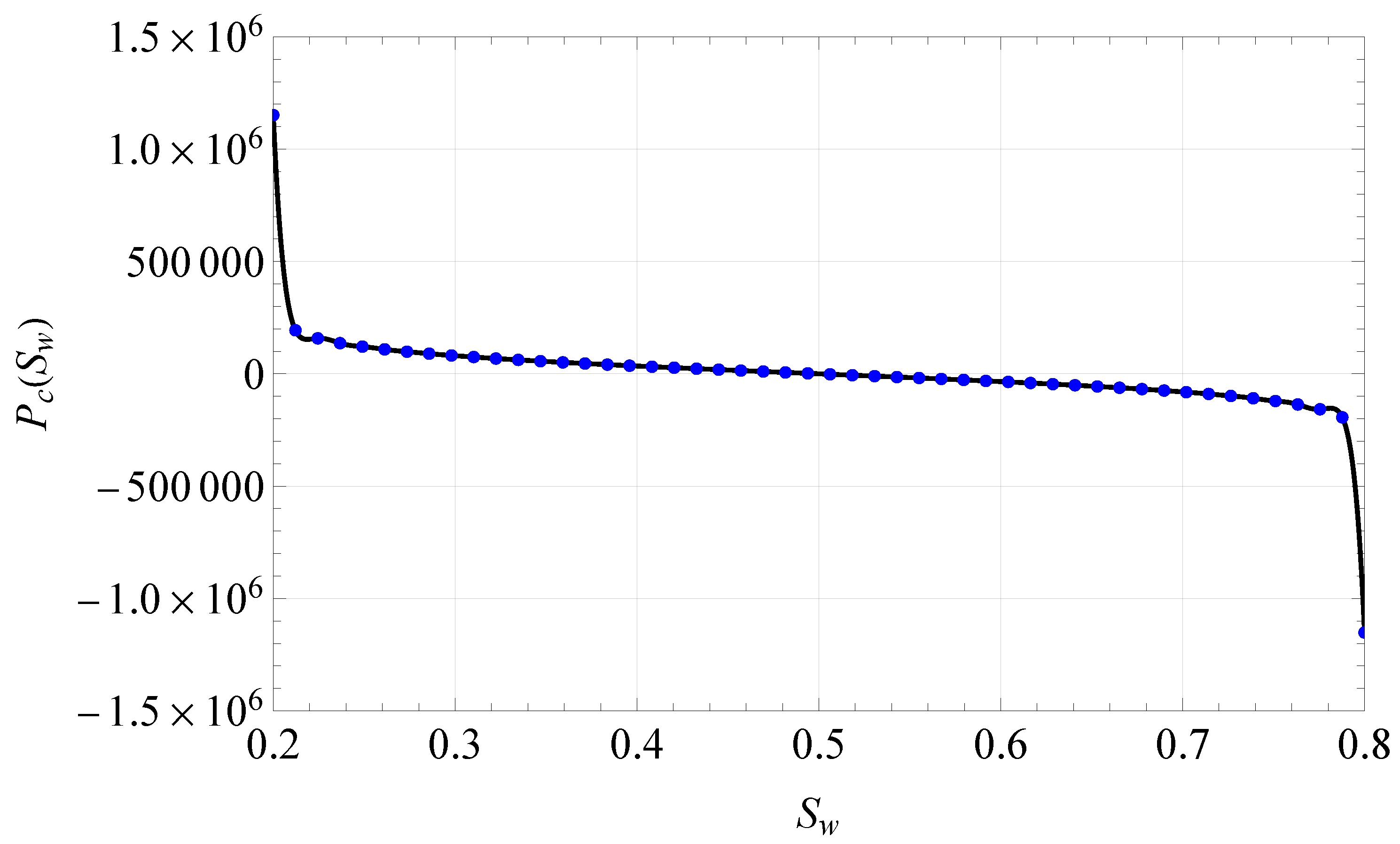
Figure 2.
Graphical illustration of the Kirchhoff transformation and its inversion, with plots of (a) versus and (b) versus .
Figure 2.
Graphical illustration of the Kirchhoff transformation and its inversion, with plots of (a) versus and (b) versus .
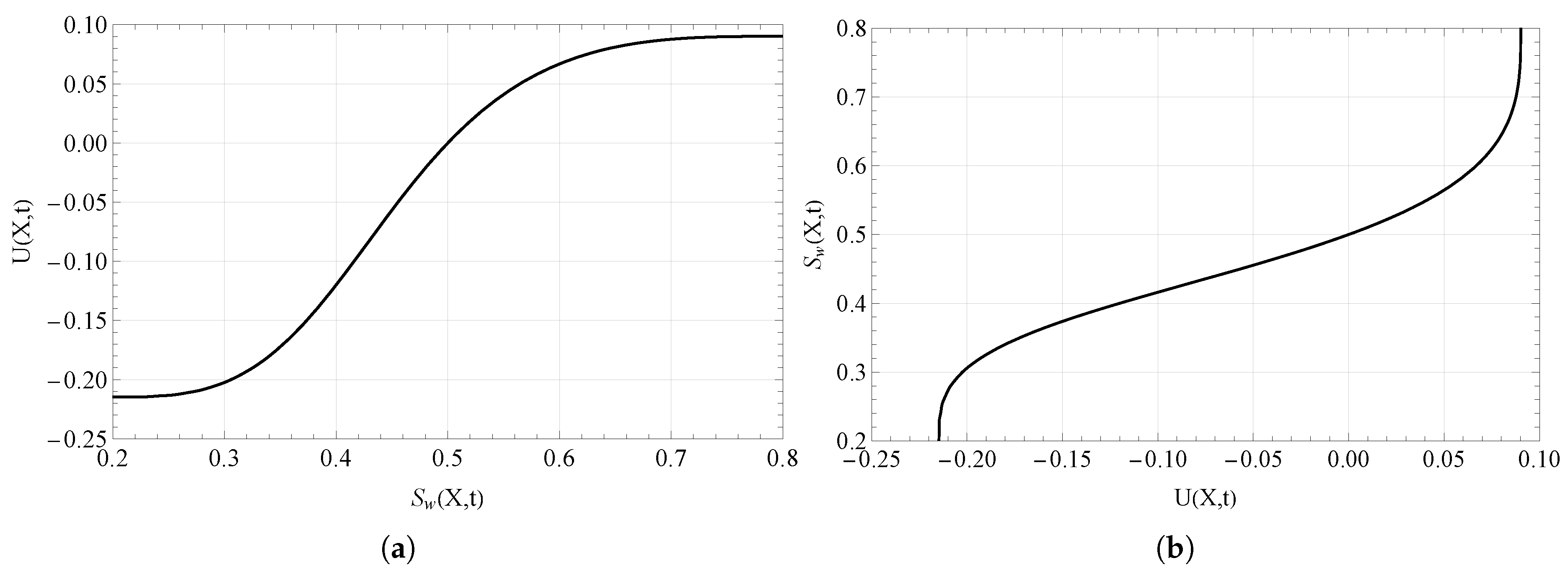
Figure 3.
Relative residue estimate for at s.
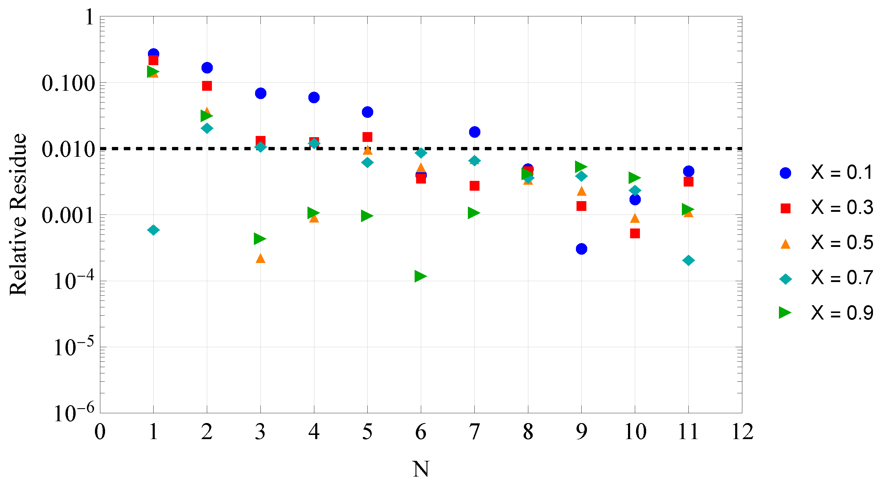
Figure 4.
Relative residue estimate for at s.
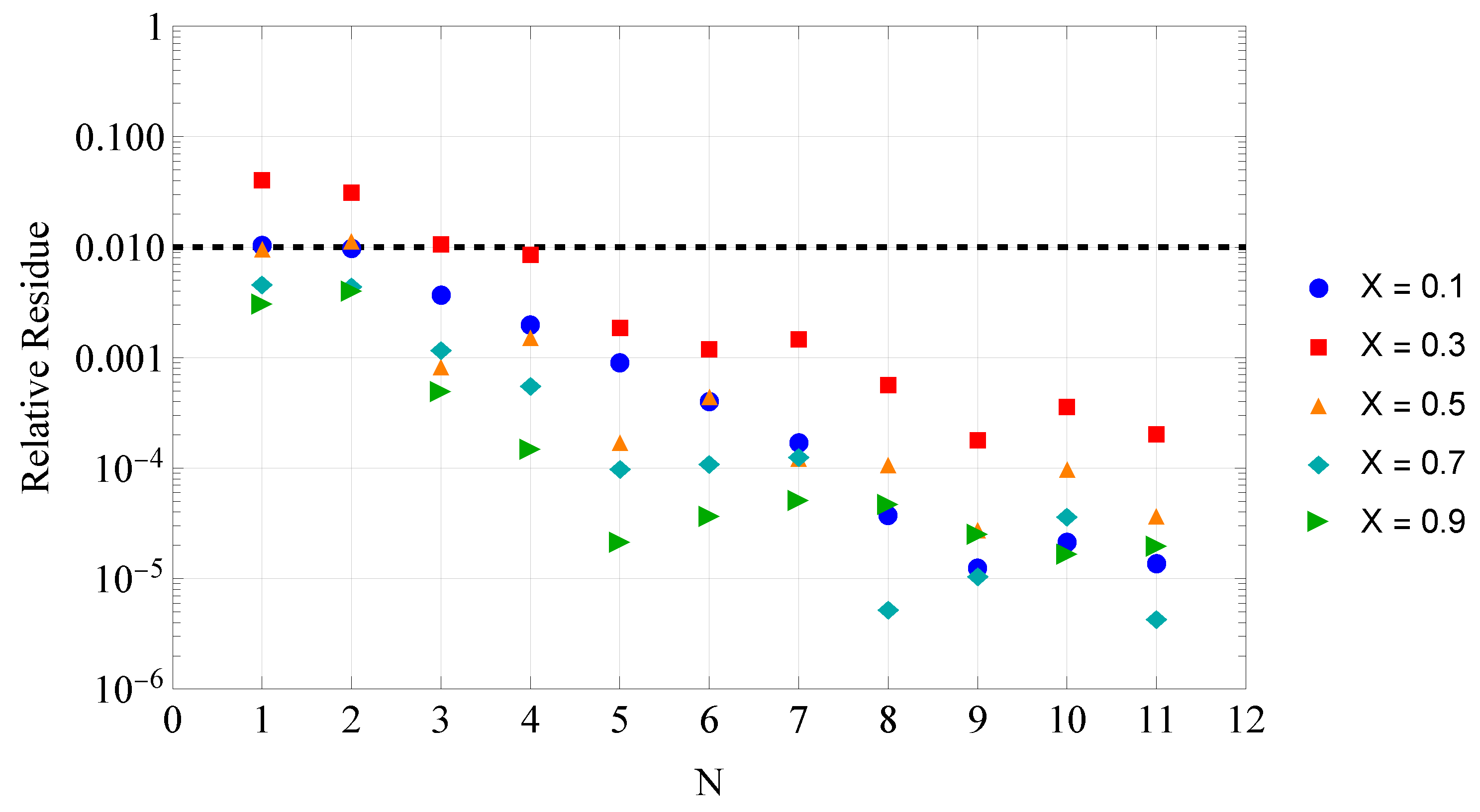
Figure 5.
Relative residue estimate for at s.
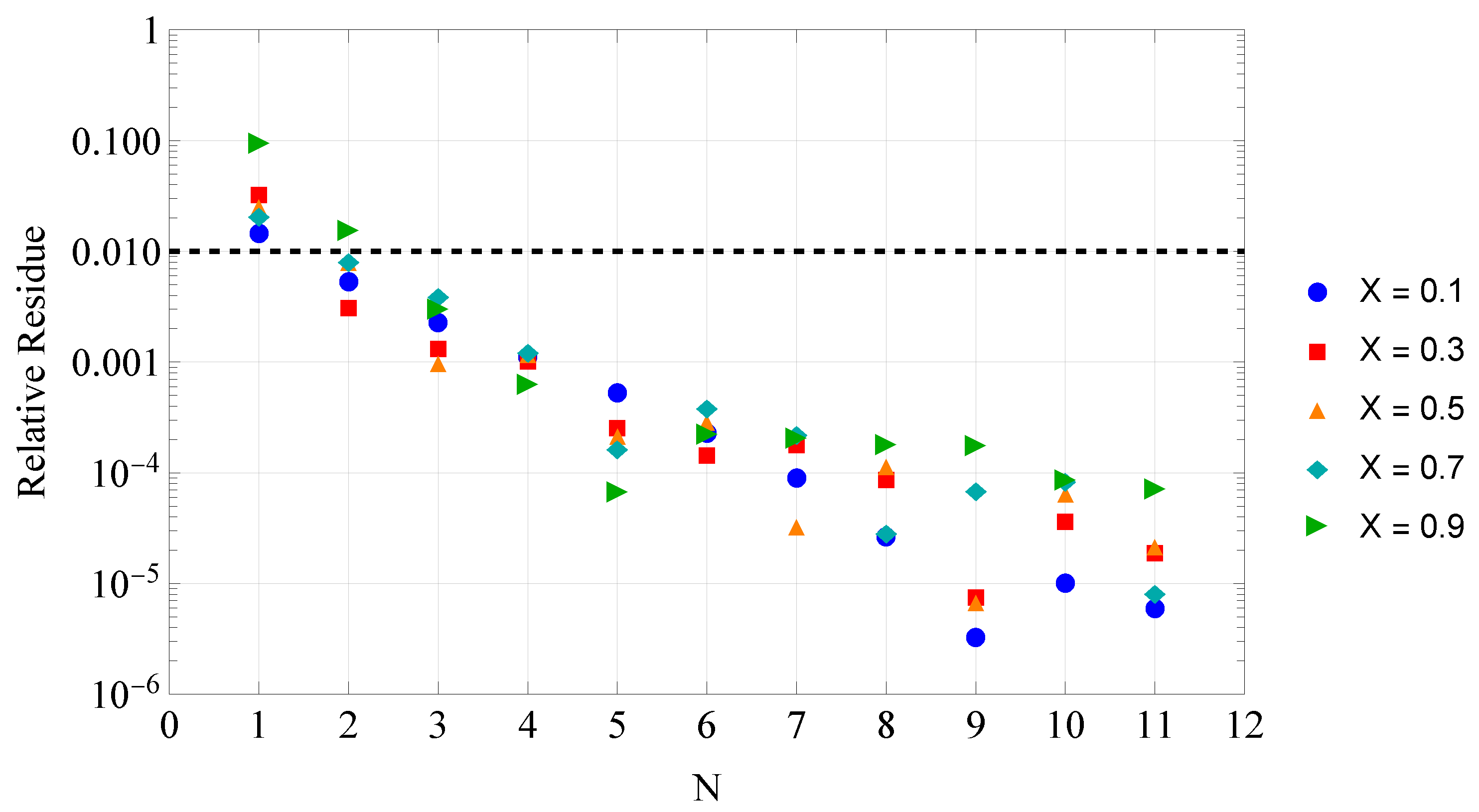
Figure 6.
Computed profiles of across the spatial domain for different time instants .
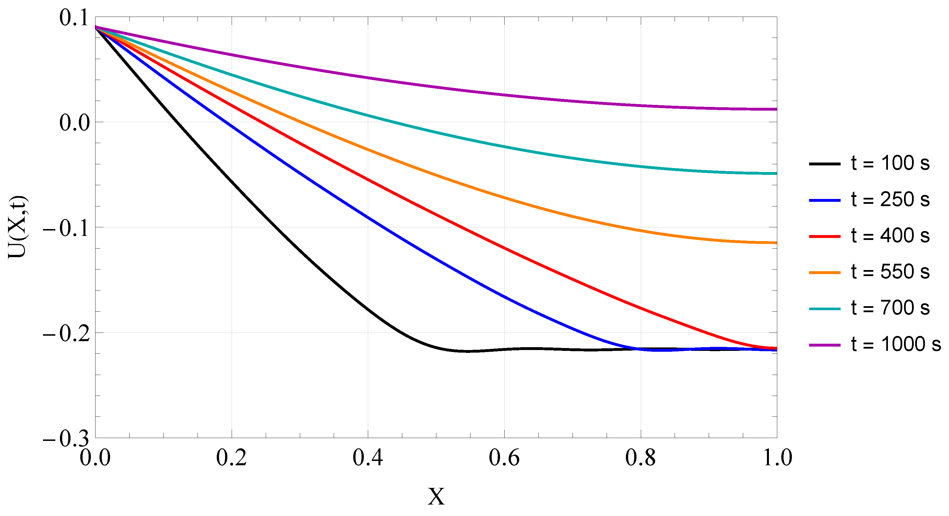
Figure 7.
Comparison of profiles computed via the GITT approach (solid lines) and the NDSolve approximate numerical solution (dashed lines), across the spatial domain and multiple time instants.
Figure 7.
Comparison of profiles computed via the GITT approach (solid lines) and the NDSolve approximate numerical solution (dashed lines), across the spatial domain and multiple time instants.
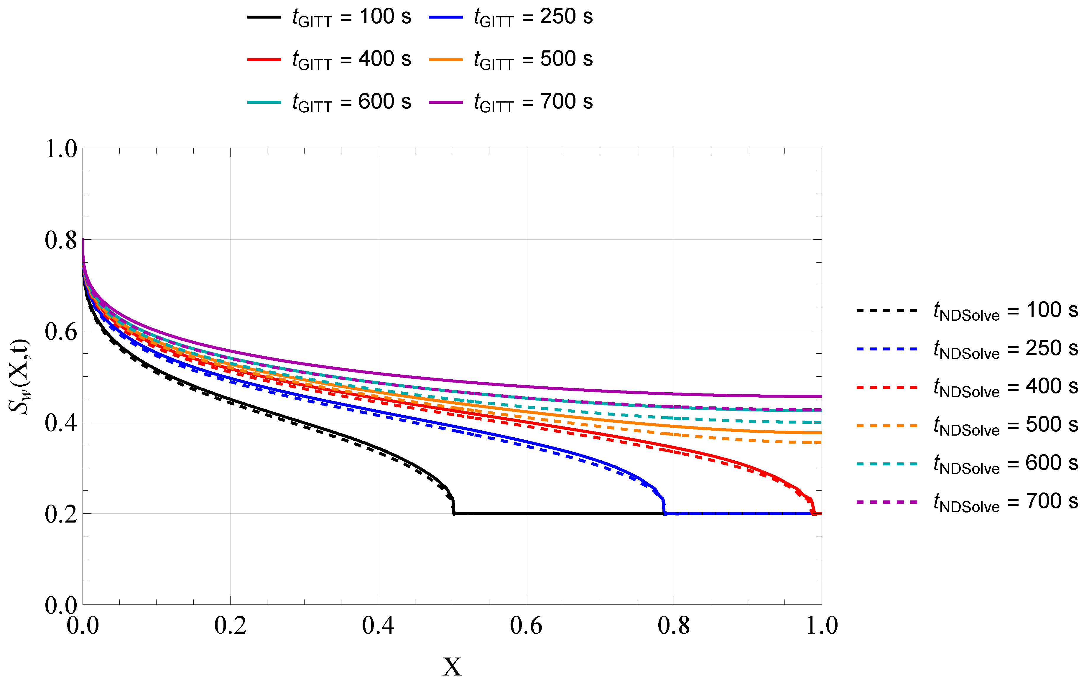
Table 1.
Physical properties and other input data.
| Property | Symbol | Value | Unit |
|---|---|---|---|
| Maximum water relative permeability | - | ||
| Maximum oil relative permeability | - | ||
| Exponent in model | 3 | - | |
| Exponent in model | 3 | - | |
| Irreducible oil saturation | - | ||
| Irreducible water saturation | - | ||
| Porosity | - | ||
| Water viscosity | kg·m−1·s−1 | ||
| Oil viscosity | kg·m−1·s−1 | ||
| Core diameter | D | m | |
| Absolute permeability | K | 100 | mD |
| Injected water flow rate | q | 1 | cm3·h−1 |
| Core length | L | m |
Table 2.
Convergence of for s and N up to 12.
| N | |||||
|---|---|---|---|---|---|
| 2 | 0.04847 | -0.03647 | -0.1162 | -0.1809 | -0.2178 |
| 4 | 0.04661 | -0.03696 | -0.1146 | -0.1815 | -0.2179 |
| 6 | 0.04667 | -0.03702 | -0.1146 | -0.1816 | -0.2179 |
| 8 | 0.04696 | -0.03764 | -0.1147 | -0.1802 | -0.2188 |
| 10 | 0.04712 | -0.03733 | -0.1146 | -0.1806 | -0.2195 |
| 12 | 0.04713 | -0.03731 | -0.1147 | -0.1807 | -0.2197 |
| Shanks | 0.04711 | -0.03736 | -0.1147 | -0.1807 | -0.2198 |
Table 3.
Convergence of for s and N up to 12.
| N | |||||
|---|---|---|---|---|---|
| 2 | 0.06305 | 0.009250 | -0.03644 | -0.06956 | -0.08694 |
| 4 | 0.06252 | 0.008871 | -0.03593 | -0.06930 | -0.08727 |
| 6 | 0.06242 | 0.008964 | -0.03601 | -0.06925 | -0.08729 |
| 8 | 0.06239 | 0.008958 | -0.03598 | -0.06926 | -0.08729 |
| 10 | 0.06239 | 0.008949 | -0.03599 | -0.06926 | -0.08728 |
| 12 | 0.06239 | 0.008951 | -0.03599 | -0.06926 | -0.08728 |
| Shanks | 0.06239 | 0.008951 | -0.03599 | -0.06926 | -0.08728 |
Table 4.
Convergence of for s and N up to 12.
| N | |||||
|---|---|---|---|---|---|
| 2 | 0.07796 | 0.05304 | 0.03312 | 0.01980 | 0.01328 |
| 4 | 0.07760 | 0.05280 | 0.03346 | 0.01994 | 0.01308 |
| 6 | 0.07752 | 0.05286 | 0.03340 | 0.01998 | 0.01306 |
| 8 | 0.07751 | 0.05286 | 0.03342 | 0.01997 | 0.01306 |
| 10 | 0.07750 | 0.05285 | 0.03341 | 0.01997 | 0.01307 |
| 12 | 0.07750 | 0.05286 | 0.03342 | 0.01997 | 0.01307 |
| Shanks | 0.07750 | 0.05285 | 0.03342 | 0.01997 | 0.01307 |
Table 8.
Convergence of for s and N up to 6 .
| N | |||||
|---|---|---|---|---|---|
| 1 | 0.5525 | 0.4573 | 0.3962 | 0.3396 | 0.2737 |
| 2 | 0.5595 | 0.4651 | 0.4018 | 0.3375 | 0.2000 |
| 3 | 0.5593 | 0.4650 | 0.4019 | 0.3377 | 0.2000 |
| 4 | 0.5569 | 0.4652 | 0.4029 | 0.3354 | 0.2000 |
| 5 | 0.5583 | 0.4645 | 0.4034 | 0.3348 | 0.2000 |
| 6 | 0.5573 | 0.4650 | 0.4030 | 0.3352 | 0.2000 |
| Shanks | 0.5577 | 0.4648 | 0.4032 | 0.3350 | 0.2000 |
| 6 (N=12) | 0.5579 | 0.4665 | 0.4056 | 0.3413 | 0.2000 |
Table 9.
Convergence of for s and N up to 6 .
| N | |||||
|---|---|---|---|---|---|
| 1 | 0.5846 | 0.5037 | 0.4598 | 0.4320 | 0.4176 |
| 2 | 0.5857 | 0.5048 | 0.4604 | 0.4318 | 0.4168 |
| 3 | 0.5848 | 0.5044 | 0.4608 | 0.4321 | 0.4165 |
| 4 | 0.5846 | 0.5044 | 0.4608 | 0.4321 | 0.4165 |
| 5 | 0.5845 | 0.5045 | 0.4608 | 0.4321 | 0.4165 |
| 6 | 0.5845 | 0.5045 | 0.4608 | 0.4321 | 0.4165 |
| Shanks | 0.5845 | 0.5045 | 0.4608 | 0.4321 | 0.4165 |
| 6 (N=12) | 0.5874 | 0.5093 | 0.4673 | 0.4408 | 0.4269 |
Table 10.
Convergence of for s and N up to 6 .
| N | |||||
|---|---|---|---|---|---|
| 1 | 0.6328 | 0.5690 | 0.5363 | 0.5174 | 0.5085 |
| 2 | 0.6297 | 0.5658 | 0.5347 | 0.5177 | 0.5102 |
| 3 | 0.6287 | 0.5654 | 0.5350 | 0.5180 | 0.5099 |
| 4 | 0.6283 | 0.5654 | 0.5351 | 0.5179 | 0.5100 |
| 5 | 0.6281 | 0.5655 | 0.5351 | 0.5179 | 0.5100 |
| 6 | 0.6281 | 0.5655 | 0.5350 | 0.5180 | 0.5100 |
| Shanks | 0.6281 | 0.5655 | 0.5350 | 0.5180 | 0.5100 |
| 6 (N=12) | 0.6302 | 0.5684 | 0.5383 | 0.5215 | 0.5137 |
Table 11.
Convergence of for s and .
| 20 | 0.5572 | 0.4649 | 0.4028 | 0.3344 | 0.2000 |
| 40 | 0.5573 | 0.4650 | 0.4030 | 0.3351 | 0.2000 |
| 60 | 0.5573 | 0.4650 | 0.4030 | 0.3351 | 0.2000 |
| 80 | 0.5573 | 0.4650 | 0.4030 | 0.3352 | 0.2000 |
| Shanks () | 0.5577 | 0.4648 | 0.4032 | 0.3350 | 0.2000 |
Table 12.
Convergence of for s and .
| 20 | 0.5843 | 0.5041 | 0.4603 | 0.4314 | 0.4156 |
| 40 | 0.5844 | 0.5044 | 0.4607 | 0.4320 | 0.4164 |
| 60 | 0.5844 | 0.5044 | 0.4607 | 0.4320 | 0.4164 |
| 80 | 0.5845 | 0.5045 | 0.4608 | 0.4321 | 0.4165 |
| Shanks () | 0.5845 | 0.5045 | 0.4608 | 0.4321 | 0.4165 |
Table 13.
Convergence of for s and .
| 20 | 0.6279 | 0.5653 | 0.5348 | 0.5177 | 0.5097 |
| 40 | 0.6280 | 0.5655 | 0.5350 | 0.5179 | 0.5099 |
| 60 | 0.6281 | 0.5655 | 0.5350 | 0.5179 | 0.5099 |
| 80 | 0.6281 | 0.5655 | 0.5350 | 0.5180 | 0.5100 |
| Shanks () | 0.6281 | 0.5655 | 0.5350 | 0.5180 | 0.5100 |
Disclaimer/Publisher’s Note: The statements, opinions and data contained in all publications are solely those of the individual author(s) and contributor(s) and not of MDPI and/or the editor(s). MDPI and/or the editor(s) disclaim responsibility for any injury to people or property resulting from any ideas, methods, instructions or products referred to in the content. |
© 2025 by the authors. Licensee MDPI, Basel, Switzerland. This article is an open access article distributed under the terms and conditions of the Creative Commons Attribution (CC BY) license (http://creativecommons.org/licenses/by/4.0/).
Copyright: This open access article is published under a Creative Commons CC BY 4.0 license, which permit the free download, distribution, and reuse, provided that the author and preprint are cited in any reuse.


