
Submitted:
19 February 2025
Posted:
20 February 2025
You are already at the latest version
Abstract
We address the numerical simulation of non-isothermal two-phase water-oil flow in oil reservoirs and deal with the problem of heavy oil recovery by heating the reservoir (via injection of heated fluid), aiming at reducing its viscosity and increasing its mobility. We write the governing equations in terms of the non-wetting phase pressure (oil), the wetting phase saturation (water), the reservoir average temperature without assuming the local thermal equilibrium hypothesis, and we consider that relative permeabilities vary with temperature. The Finite Volume Method is employed, and we linearize the resulting algebraic equations using the Picard method. The linearized discretized equations are solved sequentially to obtain the pressure, saturation, and average temperature using the Preconditioned Conjugate Gradient (pressure and average temperature) and Preconditioned Stabilized Biconjugate Gradient Method (saturation) methods. After validating the numerical results, we performed a sensitivity analysis considering a reservoir with slab geometry. The results showed the positive impact that reservoir heating has on the recovery of heavy oils.
Keywords:
Enhanced thermal recovery methods
; Finite Volume Method
; Non-isothermal flow
; Reservoir simulation
; Two-phase flow
1. Introduction
We can mention energy generation, the environment, health, and biological systems where porous media flow knowledge is significant. Specifically, we have as examples oil and gas exploitation, fuel cells, batteries, solid mechanics, and cardiovascular systems [1]. For example, numerical simulation can be used in the oil industry, which invests significant resources to reduce its costs and risks inherent to production.
We can obtain data about flow patterns by performing experiments using reservoir samples. On the other hand, information can also be collected through pressure tests in injection/producing wells and temperature and pressure data analysis. However, these are expensive and may be unfeasible when we want to study several production scenarios. For this purpose, numerical simulation becomes a valuable alternative tool [2]. In this context, we propose here to use it to solve non-isothermal two-phase flow using a one-equation model derived without assuming the hypothesis of local thermal equilibrium.
Numerical reservoir simulation requires a prior understanding of several areas of knowledge, such as mathematics, physics, numerical methods, and advanced programming [3], and it is widely used in the oil industry [2]. It is due to the inherent difficulties in accurately obtaining reservoir properties throughout its extension and the complexity of determining flow behavior in situ. Therefore, it is an ally when we need to maximize hydrocarbon recovery.
We know that the hydrocarbon production stages can be divided into primary, secondary, and tertiary [4]. In the primary, the oil or gas is obtained due to the difference in pressure between the interior of the reservoir and the surface. In the second, part of the large quantity of hydrocarbons remaining in the reservoir is recovered via the injection of an immiscible fluid, available in abundance and at low cost. Finally, we have the chemical, miscible displacement, biological, and thermal methods [5]. All aim to promote higher mobility of hydrocarbons, decreasing the resistance to their flow and promoting increased production [4].
In the case of conventional oils (API gravity greater than 30), production costs are comparatively lower than those associated with heavier oils [6]. However, due to the current depletion of their reserves, special attention has been given to exploring those with API gravity between 5 and 22. On the other hand, as they have a higher viscosity, there is higher resistance to their flow, and production costs are higher [7]. Under these circumstances, the dominant recovery techniques are thermal, non-thermal, or cold and solvent-based [8].
Therefore, an attractive alternative to increase the recovery of heavy oils is the use of so-called thermal methods [9]. For example, static heaters can be positioned inside the reservoir. As a result, there will be a decrease in its viscosity and a consequent increase in its fluidity [10].
As with other recovery techniques, we can also use numerical simulation for thermal methods [11]. The most commonly used is steam injection [12], which has the disadvantage of requiring a large amount of available water in addition to the energy cost associated with steam generation. In addition, it causes harmful effects on the environment due to the means generally used to generate the necessary energy, causing the emission of greenhouse gases [12]. An alternative, in situ combustion, has been applied with relative success in Canada [8].
We can also use electric energy to heat the reservoir by introducing heating elements that transfer heat to the fluid and the rock [7,13]. Another possibility is electromagnetic heating, enabling localized heating and being able to transfer up to 92% of the energy generated to its surroundings [14]. The number and location of the heating elements can vary to maximize the recovery process.
In the physical-mathematical modeling of porous media flow, compared to isothermal flow, we must consider the energy equation in non-isothermal flow in addition to the continuity and momentum equations. In the literature, one- or two-equation models are commonly used, with the second being the most suitable when there are significant differences in the order of magnitude of the thermal properties of the fluids and the porous matrix [15,16]. The one-equation model for single-phase flow [11,17,18] can be derived with or without assuming the hypothesis of local thermodynamic equilibrium [19]. In the case of the two-equation model [15,16], we use separate equations to obtain the temperature of the fluid and the rock, and the heat transfer between them is accounted for via a source term [20].
In the most general case, we must consider a multiphase flow due to the presence of more than one phase when using advanced recovery techniques. For example, Siavashi et al. [21] simulated the non-isothermal two-phase flow of immiscible fluids in a saturated medium, adopting the hypothesis of local thermal equilibrium, and they simulated the injection of heated water via the streamline method. On the other hand, also assuming local thermal equilibrium, Roy et al. [22] studied the non-isothermal, compositional two-phase flow, considering the presence of chemical reactions. We find other applications in Lindner et al. [23] and Kumar et al. [24]. The first dealt with cooling by phase change and used a mixing model, considering a multi-component fluid, without considering local thermal equilibrium. The last one addressed the drying process in food via microwaves, in which a fluid flow model in a porous medium with phase change was used.
Although phase changes may occur due to the temperature increase inside the reservoir, we did not consider them here. As a preventive measure, we monitored the maximum temperature values to prevent them from occurring. Therefore, the case of a three-phase flow is outside the scope. In this initial work, we will only deal with the problem of injecting a heated fluid into a reservoir with slab geometry. Later, we will attack the heating problem using static heating wells.
2. Non-Isothermal Flow in Porous Media
We present below the governing equations that will provide the saturation and average temperature of the reservoir. In addition to establishing how the properties of the fluids and the porous matrix will be calculated.
We considered the following hypotheses in the model used:
- the rock formation is anisotropic in terms of absolute permeability;
- the rock compressibility is small and constant;
- the fluids are Newtonian;
- no chemical reactions occur;
- the flow is laminar at a very low velocity;
- the fluids have a steady chemical composition;
- the flow is non-isothermal, two-phase and three-dimensional;
- the fluids are slightly compressible;
- the thermal conductivities of the rock and fluids are constant;
- and the hypothesis of local thermal equilibrium is not considered.
For two-phase flow in porous media, we we obtain from the mass balance [3]
where is the porosity, is the density, is the superficial velocity, S is the saturation, is the source term, and the subscript indicates the phase in question. Furthermore,
where is the reference porosity, determined at the reference pressure () and temperature (), is the rock compressibility coefficient, represents the rock thermal expansivity coefficient, is the pressure of the non-wetting phase (oil) and T is the mean reservoir temperature (to be defined later) [3].
Regarding density [3], we employ
where is the density of the phase under reference conditions, is the fluid compressibility coefficient, and is the thermal expansion coefficient of the phase .
Although viscosity varies depending on pressure and temperature, we will only consider its variation with temperature [11],
where and are constants determined for a given type of oil, is the reference temperature for calculating viscosity, and the water viscosity is considered constant.
In two-phase flow, Darcy’s classical law must be modified by introducing the relative permeability [3],
where is the relative permeability of phase, is the viscosity, is the absolute permeability tensor (diagonal), is the pressure, , where g is the magnitude of the acceleration due to gravity, and Z is the depth.
Since this is a non-isothermal flow, we use a model that takes into account the variation of relative permeability as a function of temperature [25]:
for the wetting phase (water), where and, for the non-wetting phase,
where , is the saturation of the wetting phase, and the temperature T should be given in oC. These correlations are valid for temperatures ranging from 70 to 220 degrees Celsius.
Combining Equations (1) and (5), we have, for each phase,
where is the formation-volume factor, and , being and the densities at standard (constant) conditions of the wetting phase (water), and of the non-wetting phase (oil), respectively.
The reservoir is saturated
and the effects of capillary pressure,
are accounted for [26]
where is the maximum capillary pressure, the exponent must be provided, is the irreducible water saturation, and is the residual oil saturation.
Therefore, by substituting Equations (10) and (11) into Equations (8) and (9) we obtain the two governing equations:
As previously stated, it is common to use the assumption of local thermal equilibrium (equality of mean temperatures of fluids and porous matrix) [22,27]. However, in some situations, it may be inappropriate [28]. As alternatives, we have the one-equation model without adopting such an assumption [19], or the two-equation model [15] or three-equations, with phase change [28] or without phase change [29]. Here, we employ the one-equation model (without local thermal equilibrium), whose dependent variable is the mean reservoir temperature (weighted average of the phase and rock temperatures), and the thermal heating is modeled via source terms [11].
For constant heat capacities, the macroscopic equation governing heat transfer is [30]:
where represents the effective thermal dispersion tensor, and are the enthalpies of oil and water, represents a volumetric thermal source (when there are heating wells), is the total volume, and and represent the volumetric mass flow rates when there are injection/producing wells.
The average temperature of the porous medium, considering both phases and the rock, is given by [30]:
where , , , and are respectively the specific heat and temperatures of the oil and water, and T represents the average reservoir temperature. Furthermore [30],
represents the average heat capacity.
The enthalpies of the fluids are calculated knowing the average temperature of the reservoir [11]:
For example, after applying the Method of Volume Averaging [31] to the energy balance equation, we see the appearance of the effective thermal dispersion tensor in the macroscopic equation describing energy transfer at the laboratory scale [19,32]. It contains the contribution of three terms related to thermal conduction, tortuosity, and hydrodynamic dispersion and, in the case of two-phase flow,
where , and are the thermal conductivities of oil, water and rock, respectively, is the identity tensor, is the tortuosity tensor, and is the hydrodynamic dispersion tensor.
We assume that the tortuosity tensor is diagonal and that its components are constant and given by [33]:
We take the hydrodynamic dispersion tensor to be diagonal and anisotropic, with its axial and transversal components determined via [32]:
where is the Péclet number. The Reynolds () and Prandtl () numbers are defined for the mobile phases (water and oil) by and , where represents the mean particle diameter of the porous medium.
2.1. Initial and Boundary Conditions
We still need to provide the initial and boundary conditions to complete the physical-mathematical model, whose governing equations are (13), (14), and (15).
We provide pressure, temperature, and saturation as initial conditions at . For pressure, their values consider the hydrostatic gradients [3]. Similarly, for temperature, geothermal energy causes it to vary at a rate of 25-30 K/km for the region of the Earth’s crust [34].
Regarding boundary conditions, Dirichlet, Neumann, or Robin-type conditions can be employed on the entire boundary or on part of it [4].
The reservoir has a slab geometry, and the main flow is in the direction of the x-axis. At the inlet boundary, we impose a pressure gradient and the temperature and saturation of the injected fluid. At the right boundary, we establish a pressure value and zero derivatives for the saturation and temperature in the flow direction. At the other boundaries, we consider zero flow conditions and zero derivatives for saturation and temperature in the directions perpendicular to the reservoir face.
3. Numerical Resolution Methodology
In solving governing differential equations, we employ the Finite Volume Method [2,35]. It is a well-known method having conservative properties that make it a good option when solving systems of partial differential equations [35]. As usual, the mean values of the dependent variables are determined at the center of the finite volumes and do not vary inside them (for a given time).
The domain of dimensions , , and is discretized using , , and finite volumes (whose dimensions, not necessarily constant, are , , and ) in the x-, y-, and z-directions, Figure 1, so that,
where the indices i, j and k indicate the blocks (cells or finite volumes) in the x-, y- and z-directions, respectively. In this system, we reference the boundaries (faces) of the blocks via the notation (), (), and () [35].
In Figure 2, we indicate the faces of the finite volumes by , , , , and . On the other hand, we use capital letters when we refer to the nodes positioned at their respective centers: , , , , , and .
Once we have generated the computational mesh, we perform space-time integration of Equations (13), (14), and (15) in each cell of the domain:
where is the time increment and the subscript V indicates that the integration domain is the control volume.
Since we chose a widely used method, we will omit the details concerning space-time integration of the governing equations [30]. We opted for a fully time implicit formulation and used space-centered difference approximations.
In the discretized equations, we introduced a new variable, , which represents the transmissibility evaluated on the faces of the finite volumes
where the subscripts e and w refer to the values that must be evaluated on the and faces, and represent the distances between the centers of the cells neighboring the finite volume considered, and is the area of the face of the finite volume. Analogous expressions are obtained for the other faces in the y- and z-directions.
Another point of fundamental importance is the approximation of transmissibilities at the interfaces of the control volumes. These terms can be highly nonlinear due to their dependence on the unknowns of the problem. This fact can generate problems with convergence, as reported in [36], and the stability of the numerical method. Knowing this context and remembering that we define the properties at the centroid of the finite volume, we must introduce appropriate approximations to overcome these issues. First, we calculate from the product between a geometric term, G, and two dependent on the dependent variables, . Then,
For example, the geometric terms appearing in the three balance equations are approximated on the east face e by
where the permeability, in turn, is determined via a harmonic mean
and the same type of approximation is used for the thermal conductivities that appear in the diffusion term of the energy equation.
The F terms can be computed in two different ways. For example, we used a centered difference scheme (uniform mesh) for those that are pressure- and temperature-dependent (weakly nonlinear)
while for the saturation-dependent terms, which are strongly nonlinear, it is done using a first-order upwind scheme. For example, for relative permeability
That is, it is the calculation of the relative permeabilities on the faces of the finite volumes. The capillary pressures on the faces are calculated analogously.
After carrying out all the steps recommended by the Finite Volume Method, we obtained the discretized form for the non-wetting phase (oil) [30]
where refers to the set of faces of the finite volume, the term is given by
and with respect to gravitational effects,
The terms coming from the transient term are given by
where .
Continuing, we present the discretized equation for the wetting phase (water) [30]
where refers to the summation on each face d and, at the same time, on each centroid of the neighboring cell D, for the same spatial direction. Furthermore, the gravity term is given by
and the other ones are
Finally, we present the discretized form of the energy equation [30]
where
and the advective, gravitational and source terms are given, respectively, by
It is worth noting that the nonlinear system formed by these three equations is coupled since the oil pressure and water saturation depend on the average temperature value.
3.1. Operator Splitting and Linearization
Since we decided to use linear algebra methods, we must linearize the system of discretized equations. To do so, we opted for the Picard Method [37],
where represents, for example, the transmissibility evaluated at time , but at the previous iterative level v. On the other hand, the dependent variables are calculated at , where is the subsequent iterative level. Therefore, we have an external iterative process linked to the Picard Method and an internal one for the numerical resolution of the system of discretized equations.
However, in the present work, we employed an Operator Splitting Method [16,38,39] to enable the unknowns of the system to be determined by solving the equations sequentially. Thus, it was possible to arbitrate the most appropriate algebraic methods for each of them [36].
We established the following resolution order [30]:
3.2. Resolution of Linear Algebraic Systems
Due to the strategy employed in solving the governing equations, the pressure and average temperature are determined via the Preconditioned Conjugate Gradient Method [4], while the saturation is obtained using the Preconditioned Stabilized Biconjugate Gradient Method [40].
The choice of preconditioned methods was based on the possibility of accelerating the convergence process of iterative methods. To this end, preconditioners constructed from the incomplete LU Factorization process were used [41].
4. Numerical Results
This section aims to present and discuss the results obtained, which are the values calculated for the variables that depend on oil pressure, water saturation, and average reservoir temperature. Before starting the discussion, we first validated the numerical method.
4.1. Numerical Verification
We focused on a non-isothermal one-dimensional flow problem to verify the accuracy of the results for two-phase flow. To this end, we used the analytical solution of a simplified dimensionless problem, the soil remediation process, which consists of injecting liquid water into a porous medium to remove the oil in the soil. The fluids are immiscible, and we did not consider the effect of capillarity on the flow.
The injection of heated water begins, and the effects of capillary pressure are disregarded. The fluids have approximately the same thermal capacity, and we neglected energy transfer by diffusion. Therefore, after simplifications [42]
subject to a Riemann-type initial condition
Therefore, the solution in terms of temperature is a discontinuity that advances through the porous region. We highlight that viscosity influences the flow pattern since it is a temperature-dependent property [42]
where is the viscosity of the non-wetting phase, is equal to 1/523, and the viscosity of the wetting phase is assumed to be 1 [42].
To determine the saturation (S), we must consider the establishment of two regions separated by the temperature discontinuity interface, one on the left (higher temperature) and the other on the right (lower temperature). Therefore [42],
for the first region, subscript 1, and
for the second region, subscript 2, and they must be solved considering the following initial condition
In Equations (53) and (54), and represent the respective flux functions that, for the adopted assumptions [42], are given by
and
The saturation and temperature profiles can be observed in Figure 3 and Figure 3, respectively, obtained with a grid containing 1,000 cells and a time increment equal to 0.0025. The figures also represent the analytical solutions determined by Moyles [42] for t=0.0625.
For temperature, a comparison between numerical and analytical results shows that the simulator correctly captured the jump that occurs at . Nevertheless, due to numerical diffusion, there is indeed a slight harmful noticeable effect. However, spurious oscillations are not present, which, according to Pletcher et al. [43], would be undesirable when solving a problem containing discontinuities in its solution, which must be reproduced numerically as accurately as possible. The temperature values are independent of those of saturation, but they modify them since the viscosity varies with the temperature.
Regarding the saturation profile, it is possible to see that, in general, we observed the same behavior for both the numerical and analytical values. In the first rarefaction, they are superimposed. However, at the end of it, it is noticed that there is a deviation, and the numerical results are below the predicted value, similar to what occurs numerically in Moyles [42]. After the first rarefaction, the saturation value remains constant until the appearance of the first shock. In the case of the analytical solution, we can see the discontinuity, but it is smoothed out due to numerical diffusion in our results. It is worth noting that the appearance of the shock is due to the change in the fluid viscosity, showing the existence of coupling of the equations. After the formation of the first shock, a second rarefaction begins, followed by the appearance of the last shock.
Despite the influence of numerical diffusion, we consider that the numerical results adequately reproduced those predicted by theory.
4.2. Sensitivity analysis
Continuing, we move on to the study of the thermal oil recovery process. We considered the problem of injecting heated water into a reservoir with a slab-type geometry. This procedure aims to sweep the oil that is still in the reservoir towards the production region, besides reducing its viscosity and favoring the flow of fluids in this region. It is a fundamental case for sensitivity analysis. It has significant relevance in the hydrocarbon recovery process, highlighting the contribution of the effects of heating in the recovery of, for example, heavy oil.
This study allows us to learn what happens in a complex process of injecting heated water into a heavy oil reservoir. Therefore, to better understand it, we focus on understanding the influence of the effect of the variation of the water injection temperature (), oil viscosity, and the water injection rate ().
We used the listed aspects as an integral part of the sensitivity analysis process. The standard model for the simulations includes a reservoir containing water and oil, with a three-dimensional geometry in the form of a parallelepiped, whose dimensions are defined by the values of its length, width, and height, respectively , , and provided in Table 1. In this table, , , and represent the permeability values in the directions of the x, y, and z axes, respectively, and is the initial value of the reservoir porosity.
Table 2, Table 3 and Table 4 also contain several parameters used in the simulations, the default case, besides the properties of the fluids and the rock. Unless explicitly mentioned, these were the values used in all simulations. In Table 2, is the initial time step, is the final time step, and is the rate of increase of the time increment (). Furthermore, indicates the initial pressure at the top of the reservoir, the initial water saturation, the maximum production time, and the initial temperature of the rock. The properties and parameters used in the simulations were based on those available in the works of the authors de Freitas [41] and dos Santos Heringer et al. [39].
4.2.1. Variation of Injected Fluid Temperature
As mentioned throughout the text, the increase in the temperature of heavy oil causes its viscosity to be reduced and the saturation curve to change. Therefore, we carried out simulations with different values of the water injection temperature to verify the behavior of pressure, saturation, temperature, and viscosity inside the reservoir. Figure 4 contains the pressure values along the x axis, obtained by injecting water at distinct temperatures and for a final production time () of 7000 days.
In Figure 4, it is possible to see that the higher the injection temperature, the higher the pressure in the reservoir, and this happens due to the reduction in oil viscosity, allowing an introduction of a greater quantity of water, which causes the reservoir pressure to increase. It is worth noting that in the inlet region on the left, the pressure on the injection face will have very similar values due to the same saturation value, which means the same equivalent relative permeability for each temperature value. At the same time, it is possible to see that there is still a difference between these values, with slightly higher pressures for lower temperatures. It is due to a higher resistance to the entry of water, resulting in a consequent increase in the inlet pressure so that the pressure gradient is maintained.
Regarding temperature, as expected, as water is injected at higher temperatures, the reservoir temperature will increase in all regions, although decreasing as a function of the distance to the injection region, leading to an increase of around 12 K between the minimum and maximum values for regions that are 100 m away from the injection boundary.
Then, from the analysis of the results shown in the figure, we can see that as the temperature of the injection fluid increases, a greater quantity of oil will be recovered, and water will be present in higher amounts in the region close to the injection boundary. We know it is a direct consequence of the decrease in oil viscosity due to the temperature increases because of the transfer of energy from the wetting phase. Ultimately, this is the practical result of thermal recovery via heated fluid injection into the reservoir. It is precisely here that we can attest to the importance of using thermal methods in heavy oil recovery. The reduction in oil viscosity provided by the heating increases sweep efficiency.
4.2.2. Oil Viscosity Variation
From the variation in oil viscosity as a function of the changes in the temperature of the injected fluid (Figure 5), we could confirm the assertions made previously. The heated fluid will cause a decrease in the viscosity of the oil due to the increase in its temperature. Since the injected water will be confined to a region that is less than 20 m from the injection boundary, the decrease in the viscosity of the oil will also be higher in this region. As a consequence, it will increase progressively as the distance increases. The diminished viscosity will increase the mobility of the oil within the reservoir. We assumed that the viscosity of the water remains constant even with the introduction of temperature variation. So, we could disregard its changes concerning those of the oil. The parameter of Equation (4) directly affects the oil viscosity. Consequently, we understood that it was worth studying its influence in determining the pressure, saturation, temperature, and oil viscosity. Unlike the previous case, where viscosity changes were confined in the heated region, we analyzed the effect of the variation in viscosity throughout the entire reservoir. We chose four different values of , and the same trends were observed compared to the previous results.
We begin analyzing the pressure curves. It can be seen that the increase in viscosity causes a considerable increase in pressure in the injection region as well as in the rest of the reservoir. This can be explained by the perception that fluid mobility is reduced with the increase in viscosity, requiring an increase in injection pressure to maintain the same pressure gradient. Therefore, the lower the oil viscosity, the lower the flow resistance and the pressure values.
Regarding the temperature results, Figure 5 shows that the higher the viscosity, the lower the temperature of the medium. We can explain this fact due to the reduction of fluid mobility. Consequently, this leads to decreasing velocity and Péclet number. Thus, the effect of heat transfer by advection is reduced in the case of flows of more viscous fluids compared to lower viscosity cases.
In addition, the results show a higher amount of residual oil when the oil is more viscous, which is explained by the higher flow resistance experienced by the more viscous fluid compared to that of lighter oils. Still, regarding the analysis of the variation in saturation, it can be observed, as expected, that for the cases of the flow of more viscous fluids, the advanced front of the injected fluid does not progress as much as in the case of less viscous fluids, advancing more slowly for more viscous oils. On the other hand, for less viscous oils, most distant regions will be reached by the injected fluid in the same period of time.
The results also confirm the effects of the parameter on the oil viscosity. It is clear that the higher its value, the higher the fluid viscosity throughout the entire reservoir. However, due to the heating of the injected fluid near the injection region, they will assume lower values and increase as the fluid is further away from the left border of the reservoir.
It is relevant to highlight that viscosity varies differently as a function of temperature for each specific oil. Therefore, unlike the injection temperature of water, we can not change the way viscosity varies unless the physical properties of the oil are modified by injecting specific products for this purpose.
4.2.3. Injection Rate Variation
The water injection rate is another fundamental parameter for this study since it defines the volume of water injected into the reservoir. The respective curves obtained by changing the injection rate can be found in Figure 6, for the variation of pressure, temperature, saturation, and viscosity.
When considering the behavior of the pressure curves for different values of the pressure gradient imposed on the injection boundary, it is clear that the curves tend to get closer to each other as the injection rate increases. Therefore, it can be seen that due to the values of the reservoir and fluid properties, such as absolute permeability, porosity, and viscosity, there is a limit for the reservoir to produce under the prevailing conditions (initial pressure and temperature, fluid, and rock formation properties), remembering that the pressure is prescribed and kept constant at the production boundary. However, an influence is noted in the region close to the injection boundary due to the increase in the injection rate, which ceases to be relevant as the rate increases.
From Figure 6, regarding the temperature curves, it is not difficult to conclude that the variation in the injection rate of the heated fluid did not cause significant changes in the average temperature values inside the reservoir. Therefore, we should not expect effective changes in the oil viscosity values.
When analyzing the results regarding the saturation curves, the beneficial effect of the initial increase in the injection rate becomes evident, with the consequent increase in the swept efficiency. However, as mentioned, this effect is seen from a gradient corresponding to 15 kPa/m, and the saturation curves become increasingly closer. Therefore, the volume of residual oil in the swept region tends to have the same value for higher injection rates.
For the cases evaluated, based on what has already been explained about the variation in temperature inside the reservoir, we verify that the viscosity curves are practically the same regardless of the injection rate values.
5. Conclusions
In this work, we developed a numerical simulator to solve the problem of non-isothermal three-dimensional two-phase flow in an oil reservoir, and we solved the subsystems for oil pressure, water saturation, and average temperature sequentially. The coefficients of the equations that appear in these subsystems are linearized using the Picard method, and we calculated implicitly pressure and the water saturation. When calculating the average temperature, we did not consider the hypothesis of local thermal equilibrium, and we also used an implicit formulation in time. The effects of tortuosity and hydrodynamic dispersion are taken into account.
The numerical code was validated based on a problem already known in the literature and that has an analytical solution. From its resolution, it was possible to verify the numerical convergence and that the numerical results reproduced those provided by theory. However, we observed a small smoothing due to numerical diffusion caused by the first-order upwind scheme.
Unquestionably, the variation of the injection temperature proved to be the more efficient technique with regard to oil recovery for the cases we tested in the sensitivity analysis, taking into account the value of water saturation at the end of the rarefaction curve. For higher temperatures, there is a reduction in viscosity and the amount of oil found in the region swept by the heated water.
In the other cases, we did not obtain comparable practical gains in swept efficiency despite the reduction in oil viscosity. In the first test case, variation of the injected fluid temperature, the water saturation immediately before the discontinuity, which defines the position of the advancing front, went from approximately 0.55 to 0.65 for the lowest and highest values of water injection temperature, an increase of about 18%.
Overall, the sequential method and the methodologies for discretization, linearization, and solution of algebraic systems proved to be effective when applied to the problem of non-isothermal two-phase flow.
Author Contributions
Conceptualization, G.d.S. and H.P.A.S.; methodology, M.M.d.F., G.d.S and H.P.A.S.; software, J.D.d.S.H., M.M.d.F. and G.d.S.; validation, J.D.d.S.H., G.d.S. and H.P.A.S.; formal analysis, J.D.d.S.H., M.M.d.F., G.d.S and H.P.A.S.; investigation, J.D.d.S.H., M.M.d.F., G.d.S and H.P.A.S.; resources, J.D.d.S.H., M.M.d.F., G.d.S and H.P.A.S.; data curation, J.D.d.S.H., M.M.d.F., G.d.S and H.P.A.S.; writing—original draft preparation, H.P.A.S; writing—review and editing, J.D.d.S.H., M.M.d.F., G.d.S and H.P.A.S.; visualization, J.D.d.S.H.; supervision, G.d.S and H.P.A.S.; project administration, G.d.S and H.P.A.S.; funding acquisition, G.d.S and H.P.A.S. All authors have read and agreed to the published version of the manuscript.
Funding
This research was funded by Carlos Chagas Filho Foundation for Research Support of the State of Rio de Janeiro (FAPERJ) grant numbers E-26/010.001790/2019, E-26/010.002226/2019, E-26/211.776/2021, and E-26/210.476/2024.
Data Availability Statement
Data will be available on request.
Acknowledgments
The authors gratefully thanks Rio de Janeiro State University, Coordination for the Improvement of Higher Education Personnel (CAPES) - Finance Code 001, and National Council for Scientific and Carlos Chagas Filho Foundation for Research Support of the State of Rio de Janeiro (FAPERJ) for their support.
Conflicts of Interest
The authors declare no conflicts of interest.
References
- Das, K.M.; Mukherjee, P.P.; Muralidhar, K. Modeling Transport Phenomena in Porous Media with Applications; Springer International Publishing AG: Switzerland, 2018. [Google Scholar]
- Islam, M.R.; Moussavizadegan, S.H.; Mustafiz, S.; Abou-Kassem, J.H. Advanced Petroleum Reservoir Simulation; Wiley: Trondheim, Norway, 2010. [Google Scholar]
- Ertekin, T.; Abou-Kassem, J.; King, G. Basic Applied Reservoir Simulation; Society of Petroleum Engineers: Richardson, USA, 2001. [Google Scholar]
- Chen, Z.; Huan, G.; Ma, Y. Computational Methods for Multiphase Flows in Porous Media; Society of Industrial and Applied Mathematics: Philadelphia, USA, 2006. [Google Scholar]
- Manichand, R. Análise do Desempenho do Aquecimento Eletromagnético na Recuperação de Reservatórios de Petróleo. Master’s thesis, UFRN, Natal/RN, Brasil, 2002.
- Petitfrere, M. EOS based simulations of thermal and compositional flows in porous media. PhD thesis, Universit de Pau et des Pays de l’Adours, 2014.
- Carrizales, M.A. Recovery of Stranded Heavy Oil by Electromagnetic Heating. PhD thesis, The University of Texas at Austin, 2010.
- Aydin, H.; Nagabandi, N.; Temizel, C.; Jamal, D. Heavy Oil Reservoir Management - Latest Technologies and Workflows, Bakersfield, California, USA, 2022; Vol. SPE 209328.
- Eduardo, R. A comprehensive model describing temperature behavior in horizontal wells: Investigation of potential benefits of using downhole distributed temperature measurement system. PhD thesis, The Pennsylvania State University, 2010.
- Aouizerate, G.; Durlofsky, L.J.; Samier, P. New models for heater wells in subsurface simulations, with application to the in situ upgrading of oil shale. Computational Geoscience 2012, 16, 519–531. [Google Scholar] [CrossRef]
- Rousset, M. Reduced-order modeling for thermal simulation. Master’s thesis, University of Stanford, Stanford, USA, 2010.
- Lee, J.; Babadagli, T. Mitigating greenhouse gas intensity through new generation techniques during heavy oil recovery. Journal of Cleaner Production 2021, 286, 124980. [Google Scholar] [CrossRef]
- Rangel-German, E.R.; Schembre, J.; Sandberg, C.; Kovscek, A.R. Electrical-heating-assisted recovery for heavy oil. Journal of Petroleum Science and Engineering 2004, 45, 213–231. [Google Scholar] [CrossRef]
- Sivakumar, P.; Krishna, S.; Hari, S.; Vij, R.K. Electromagnetic heating, an eco-friendly method to enhance heavy oil production: A review of recent advancements. Environmental Technology & Innovation 2020, 20, 101100. [Google Scholar] [CrossRef]
- Moyne, C.; Amaral Souto, H.P. Multi-scale approach for conduction heat transfer: one- and two-equation models. Part 1: theory. Computational and Applied Mathematics 2014, 33, 257–274. [Google Scholar] [CrossRef]
- dos Santos Heringer, J.D.; Debossam, J.G.S.; Souza, G.; Amaral Souto, H.P. Numerical simulation of non-isothermal flow in oil reservoirs using a two-equation model. Coupled Systems Mechanics an International Journal 2019, 8, 147–168. [Google Scholar] [CrossRef]
- Rousset, M.A.H.; Huang, C.K.; Klie, H.; Durlofsky, L.J. Reduced-order modeling for thermal recovery processes. Computational Geosciences 2014, 18, 401–415. [Google Scholar] [CrossRef]
- Heringer, J.D.S.; Debossam, J.G.; Honório Junior, P.T.; Souza, G.; Amaral Souto, H.P. Simulação Numérica de Escoamento Não-Isotérmico em Reservatórios de Petróleo. In Proceedings of the Encontro Nacional de Modelagem Computacional, Nova Friburgo, RJ, Brasil; 2017. [Google Scholar]
- Moyne, C.; Didierjean, S.; Amaral Souto, H.P.; da Silveira, O. Thermal dispersion in porous media: one-equation model. International Journal of Heat and Mass Transfer 2000, 43, 3853–3867. [Google Scholar] [CrossRef]
- Lampe, V. Modelling Fluid Flow and Heat Transport in Fractured Porous Media. Master’s thesis, University of Bergen, Noruega, 2013.
- Siavashi, M.; Blunt, M.J.; Raisee, M.; Pourafshary, P. Three-dimensional streamline-based simulation of non-isothermal two-phase flow in heterogeneous porous media. Computers & Fluids 2014, 103, 116–131. [Google Scholar] [CrossRef]
- Roy, T.; Jönsthövel, T.B.; Lemon, C.; Wathen, A.J. A Constrained Pressure-Temperature Residual (CPTR) Method for non-isothermal multiphase flow in porous media. SIAM Journal on Scientific Computing 2020, 42, B1014–B1040. [Google Scholar] [CrossRef]
- Lindner, F.; Pfitzner, M.; Mundt, C. Multiphase, multicomponent flow in porous media with local thermal non-equilibrium in a multiphase mixture model. Transport in Porous Media 2016, 112, 313–332. [Google Scholar] [CrossRef]
- Kumar, C.; Joardder, M.U.; Farrell, T.W.; Karim, M.A. Multiphase porous media model for intermittent microwave convective drying (IMCD) of food. International Journal of Thermal Sciences 2016, 104, 304–314. [Google Scholar] [CrossRef]
- Esmaeili, S.; Sarma, H.; Harding, T.; Maini, B. Effect of Temperature on Bitumen/Water Relative Permeability in Oil Sands. Energy & Fuels 2020, 34, 12314–12329. [Google Scholar] [CrossRef]
- Ezekwe, N. Petroleum Reservoir Engineering Practice; Prentice Hall: Westford, USA, 2010. [Google Scholar]
- Bortolozzi, H.; Deiber, J. Comparison between two- and one-field models for natural convection in porous media. Chemical Engineering Science 2001, 56, 157–172. [Google Scholar] [CrossRef]
- Duval, F.; Fichot, F.; Quintard, M. A local thermal non-equilibrium model for two-phase flows with phase-change in porous media. International Journal of Heat and Mass Transfer 2004, 47, 613–639. [Google Scholar] [CrossRef]
- Petit, F.; Fichot, F.; Quintard, M. Écoulement diphasique en milieu poreux: modèle à non-équilibre local. International Journal of Thermal Science 1999, 38, 239–249. [Google Scholar] [CrossRef]
- dos Santos Heringer, J.D. Simulação de Escoamentos Bifásicos Água-Óleo Tridimensionais Não-isotérmicos em Reservatórios de Petróleo. PhD thesis, Universidade do Estado do Rio de Janeiro, 2022.
- Whitaker, S. The Method of Volume Average. Theory and Applications of Transport in Porous Media; Kluwer Academic Publishers, 1999.
- Kaviany, M. Principles of Heat Transfer in Porous Media; Springer-Verlag New York Inc.: New York, USA, 1991. [Google Scholar]
- Fu, J.; Thomas, H.R.; Li, C. Tortuosity of porous media: Image analysis and physical simulation. Earth-Science Reviews 2021, 212, 103439. [Google Scholar] [CrossRef]
- Ingvar, B.F.; Bertani, R.; Huenges, E.; Lund, J.W.; Ragnarsson, A.; Rybach, L. The possible role and contribution of geothermal energy to the mitigation of climate change. In Proceedings of the IPCC Scoping Meeting on Renewable Energy Sources, Lübeck, Germany; 2008. [Google Scholar]
- Versteeg, H.K.; Malalasekera, W. An introduction to Computational Fluid Dynamics: the finite volume method; Pearson, 2007.
- Jiang, J.; Tchelepi, H. Nonlinear acceleration of sequential fully implicit (SFI) method for coupled flow and transport in porous media. Computer Methods in Applied Mechanics and Engineering 2019, 352, 246–275. [Google Scholar] [CrossRef]
- Nick, H.M.; Raoof, A.; Centler, F.; Thullner, M.; Regnier, P. Reactive dispersive contaminant transport in coastal aquifers: Numerical simulation of a reactive henry problem. Journal of Contaminant Hydrology 2013, 145, 90–104. [Google Scholar] [CrossRef]
- Vennemo, S.B. Multiscale Simulation of Thermal Flow in Porous Media. Master’s thesis, Norwegian University of Science and Technology, Trondheim, Norway, 2016.
- dos Santos Heringer, J.D.; de Souza, G.; Amaral Souto, H.P. On the numerical simulation of non-isothermal heavy oil flow using horizontal wells and horizontal heaters. Brazilian Journal of Chemical Engineering 2023. [Google Scholar] [CrossRef]
- Saad, Y. Iterative Methods for Sparse Linear Systems, 2 ed.; SIAM: Philadelphia, 2003. [Google Scholar]
- de Freitas, M.M. Estudo Comparativo das Estratégias de Solução Numérica para Escoamentos Bifásicos em Reservatórios de Petróleo. PhD thesis, UERJ, 2017.
- Moyles, I. Thermo-Viscous Fingering in Porous Media and In-Situ Soil Remediation. Master’s thesis, The Faculty of Graduate Studies, The University of British Columbia, 2011.
- Pletcher, R.; Tannehill, J.; Anderson, D. Computational Fluid Mechanics and Heat Transfer; 3rd ed., CRC Press: New York, USA, 2013. [Google Scholar]
Figure 1.
Three-dimensional mesh.
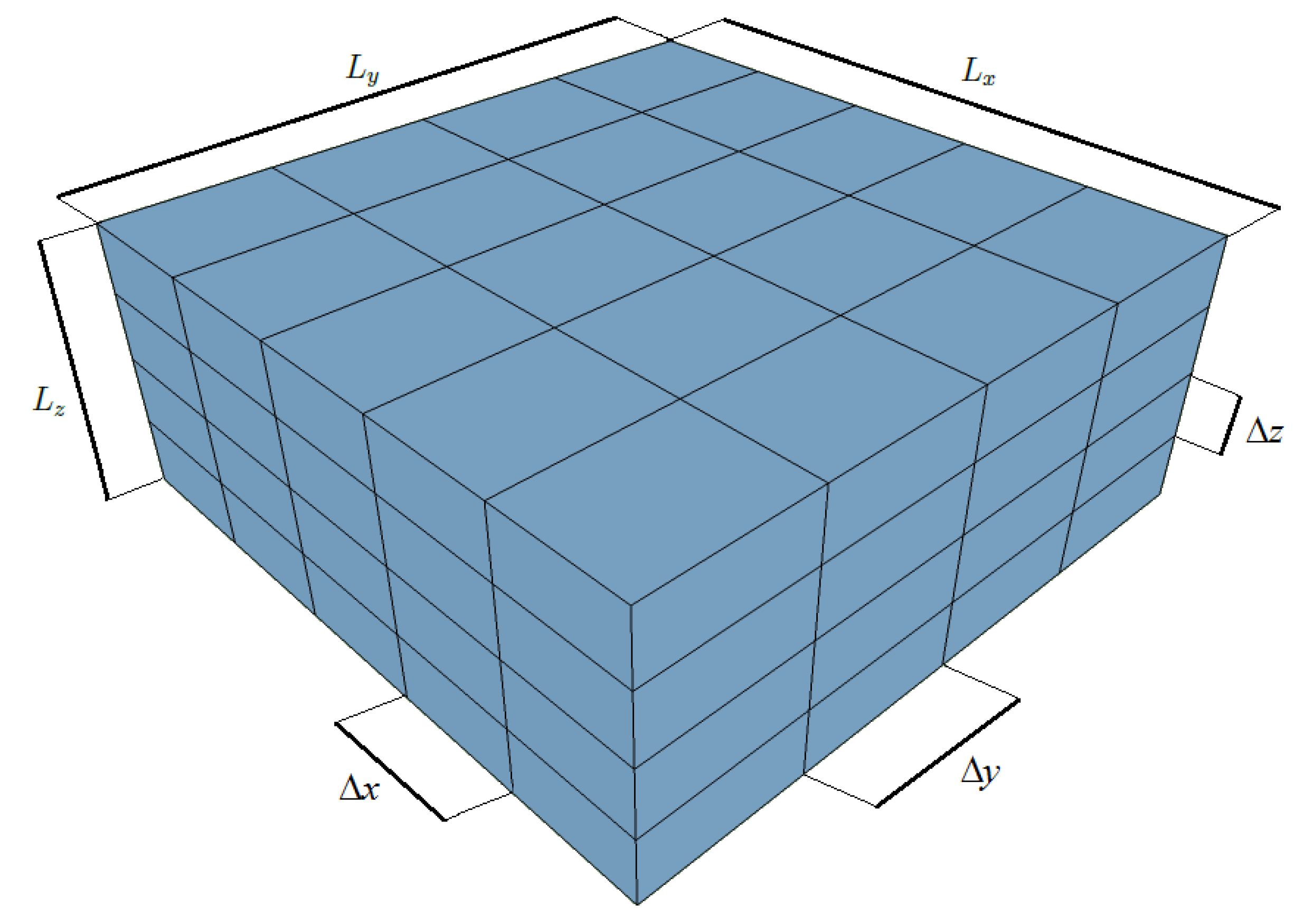
Figure 2.
Finite volume.
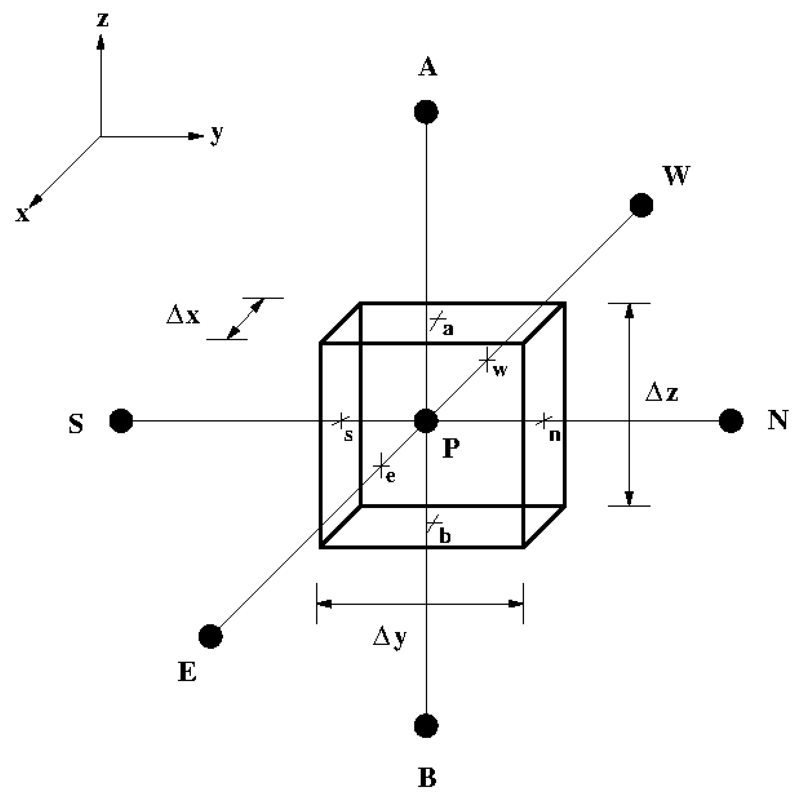
Figure 3.
Profiles of temperature and saturation at t=0,0625.
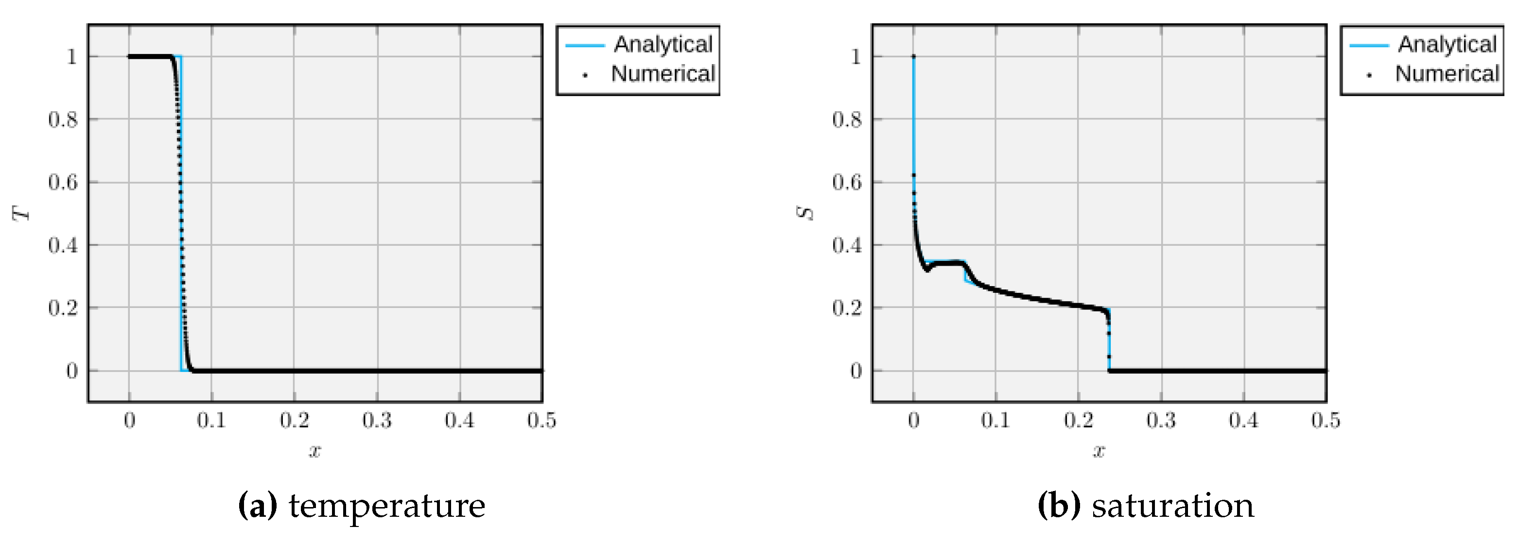
Figure 4.
From top to bottom and from left to right: distribution of pressure, temperature, saturation and oil viscosity in the x-direction, considering different values of and t=7000 days.
Figure 4.
From top to bottom and from left to right: distribution of pressure, temperature, saturation and oil viscosity in the x-direction, considering different values of and t=7000 days.
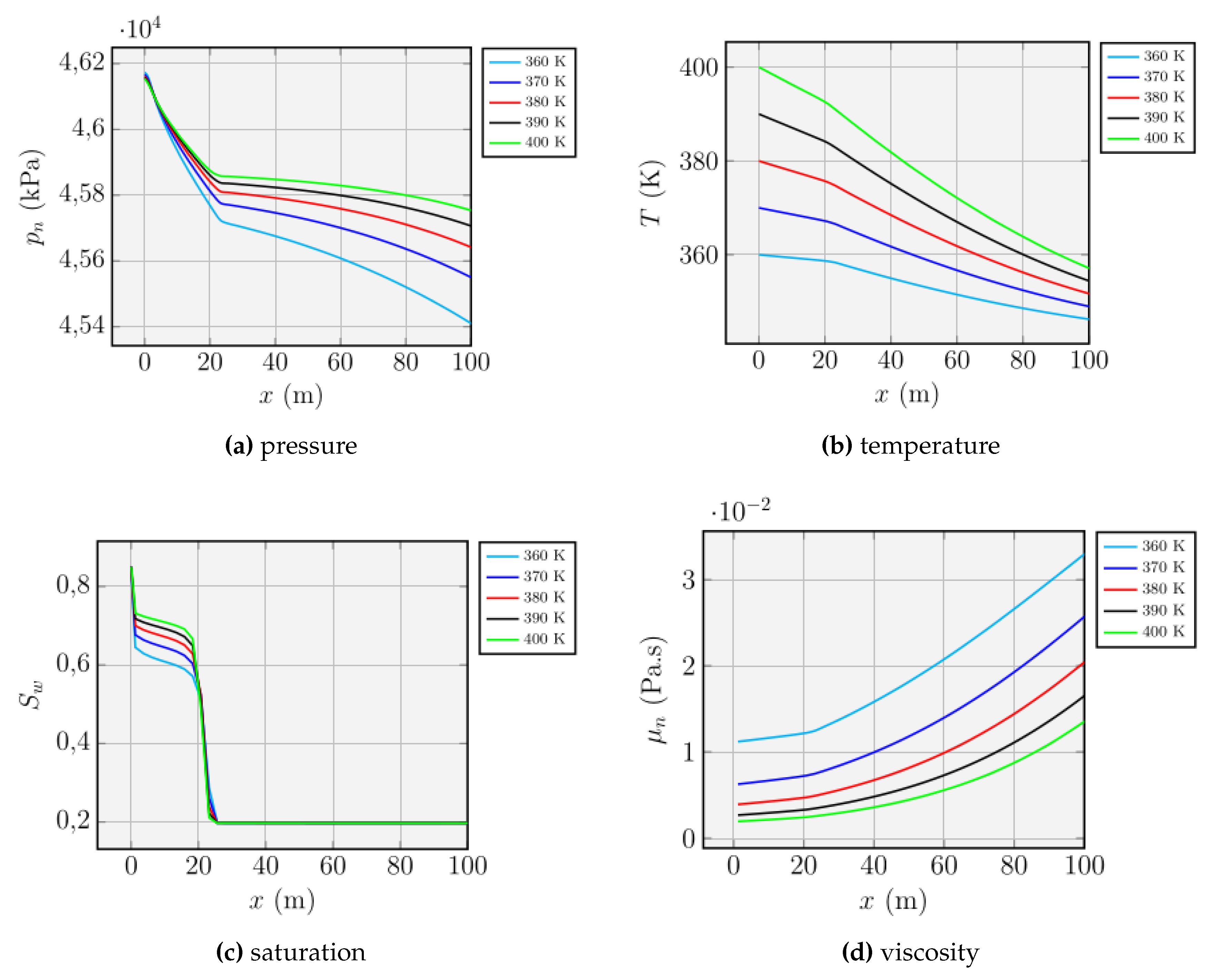
Figure 5.
From top to bottom and from left to right: distribution of pressure, temperature, saturation and oil viscosity in the x-direction, considering different values of (Equation (4)) and t=7000 days.
Figure 5.
From top to bottom and from left to right: distribution of pressure, temperature, saturation and oil viscosity in the x-direction, considering different values of (Equation (4)) and t=7000 days.
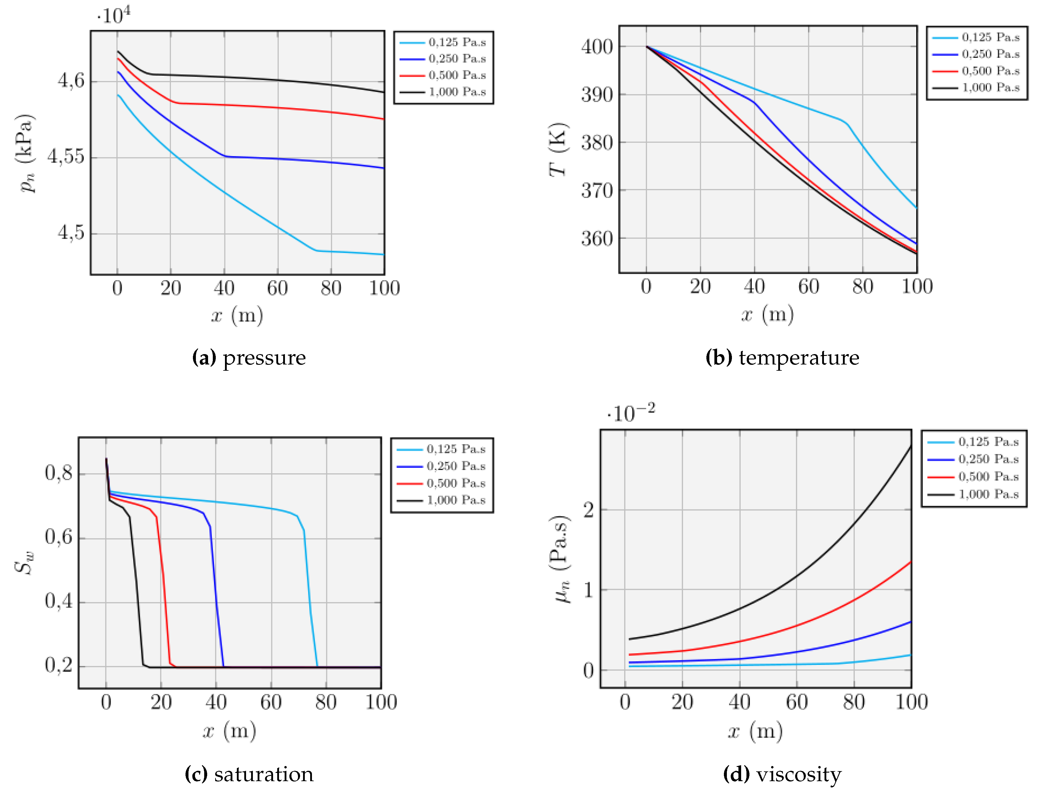
Figure 6.
From top to bottom and from left to right: distribution of pressure, temperature, saturation and oil viscosity in the x-direction, considering different values of the injection rate and t=7000 days.
Figure 6.
From top to bottom and from left to right: distribution of pressure, temperature, saturation and oil viscosity in the x-direction, considering different values of the injection rate and t=7000 days.
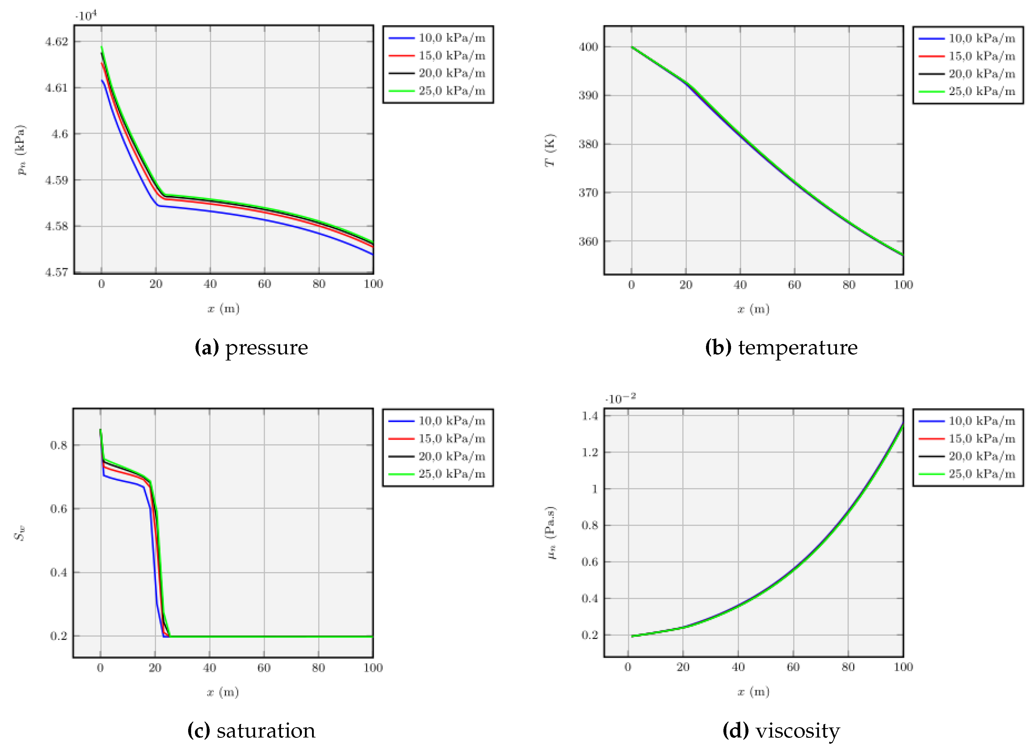

Table 1.
Parameters for the reservoir.
| Parameter | Value | Unit |
|---|---|---|
| 2.9 10−15 | m2 | |
| 7.35 10−16 | m2 | |
| 609.6 | m | |
| 304.0 | m | |
| 30,4 | m | |
| 0.2 | - |
Table 2.
Parameters for numerical simulations.
| Parameter | Value | Unit |
|---|---|---|
| 1.1 | - | |
| 250 | - | |
| 50 | - | |
| 5 | - | |
| 4.0 104 | kPa | |
| 4.0 104 | kPa | |
| 0.2 | - | |
| 0.85 | - | |
| 7000 | day | |
| 400 | K | |
| 340 | K | |
| 1.0 10−2 | day | |
| 10 | day | |
| -10 | kPa/m | |
| 0.0 | - | |
| 0.0 | K/m |
Table 3.
Parameters for fluids.
| Parameter | Value | Unit |
|---|---|---|
| 5.0 10−5 | Pa.s | |
| 444.4 | K | |
| 1.13 | - | |
| 1.022 | - | |
| 7.25 10−7 | kPa−1 | |
| 1.2 10−3 | K−1 | |
| 1700 | J.K−1.Kg | |
| 4128.18 | J.K−1.Kg | |
| 2.61 10−6 | kPa−1 | |
| 2.07 10−5 | K−1 | |
| 277.78 | K | |
| 0.1225 | W.m−1.K−1 | |
| 0.6 | W.m−1.K−1 | |
| 0.00069 | Pa.s | |
| 959 | kg/m3 | |
| 1000 | kg/m3 |
Table 4.
Parameters for the porous matrix.
| Parameter | Value | Unit |
|---|---|---|
| 1200 | J.K−1.Kg | |
| 1.8 10−5 | K−1 | |
| 5.8 10−7 | kPa−1 | |
| 1.0 10−4 | m | |
| 2 | - | |
| 4 | - | |
| 39.98 | kPa | |
| 0.15 | - | |
| 0.15 | - | |
| 4.5 | W.m−1.K−1 | |
| 2500 | kg/m3 | |
| 30 | K/km |
Disclaimer/Publisher’s Note: The statements, opinions and data contained in all publications are solely those of the individual author(s) and contributor(s) and not of MDPI and/or the editor(s). MDPI and/or the editor(s) disclaim responsibility for any injury to people or property resulting from any ideas, methods, instructions or products referred to in the content. |
© 2025 by the authors. Licensee MDPI, Basel, Switzerland. This article is an open access article distributed under the terms and conditions of the Creative Commons Attribution (CC BY) license (http://creativecommons.org/licenses/by/4.0/).
Copyright: This open access article is published under a Creative Commons CC BY 4.0 license, which permit the free download, distribution, and reuse, provided that the author and preprint are cited in any reuse.


