Submitted:
02 July 2025
Posted:
04 July 2025
You are already at the latest version
Abstract
The Power-Normal (PN) distribution was first introduced by Goto et al. in the context of modeling original observations following the application of the inverse Box–Cox (BC) transformation. This family includes the normal and log-normal distributions as special cases. In this paper, we present results for the exact Maximum Likelihood Estimation (MLE) of the PN distribution and compare them with those obtained using the truncated MLE method originally proposed by Box and Cox, implemented here by jointly maximizing all three parameters. The algorithm we propose focuses on the interval [0,1] and employs a partitioning strategy to generate initial values for the Newton–Raphson (N-R). For the exact MLE, we consider two scenarios: one in which all parameters are estimated simultaneously, and another in which only λ is optimized. We find the first approach to outperform the second overall, although both yield similar accuracy for the estimation of λ. In contrast, the truncated MLE method performs worse than the exact MLE in estimating λ, but better in the average Mean Square Error (MSE) statistic than the exact maximizing in λ alone.
Keywords:
power normal
; Box-Cox transformation
; maximum likelihood estimation
1. Introduction
The Box-Cox (BC) transformation [9] of a positive random variable is defined by
where is the transformation parameter. Note that the data must be strictly positive, which implies that Y is bounded below by . When the transformation is successful, Y is approximately normally distributed with mean and standard deviation . The probability distribution of the original variable X is known as the PN distribution, first introduced by Goto and Inoue [8], who also provided expressions for its moments in the form of power series.
The PN probability density function (PDF) is given by
where and . The function serves as a normalization constant and is defined as , 1, or depending on whether is positive, zero, or negative, respectively. The parameter k, which acts as a shape parameter of the distribution, is given by and therefore depends on all three parameters. Here, denotes the standard normal cumulative distribution function (CDF), and its derivative is the standard normal probability density function (PDF). The inverse Box–Cox transformation for a truncated normal (TN) variable Y, when , is given by .
The PN distribution in the context of the BC transformation was also studied in [10], where expressions for the mean, variance, and quantile functions were derived, and a quantile-based measure of skewness was introduced to show that the PN family is ordered with respect to the transformation parameter. Furthermore, the same paper demonstrates, using Chebyshev–Hermite polynomials, that the correlation coefficient is smaller on the PN scale.
In [1], a formula for the ordinary moments is provided, and the marginal and conditional probability density functions are derived. Additionally, the correlation curve is computed and fitted to a power law model.
For further information and analysis on the PN distribution, see [2,11], and for the BC transformation, see [5].
This paper is organized as follows. In Section 2, we present the log-likelihood function for the PN distribution and provide formulas for estimating and . We also describe the procedures followed in detail. We recall that the maximum likelihood (ML) estimator of the parameter is asymptotically normal, and we specify its asymptotic distribution. Subsequently, we derive the recursive relation for the N-R method applied to this maximization problem. Furthermore, we present the gradient vector and the Hessian matrix of the log-likelihood function with respect to the parameters , , and , as used in the implementation of the estimation algorithm. In Section 3, we describe the simulation procedure employed to generate the data sets for parameter estimation and then report and interpret the results. Finally, in Section 4, we summarize the main conclusions and suggest directions for future research concerning the PN distribution.
2. Maximum Likelihood Estimation in the PN Distribution
In this section, we revisit the MLE in the context of the PN distribution. Following Goto et al. [4], we consider two estimation methods: the truncated Log-likelihood method () and the exact Log-likelihood method (). For the former, we report only the estimation results; for the latter, we provide a full methodological description along with a comprehensive simulation study. Within the approach, we compare two scenarios: one in which all three parameters are estimated jointly (), and another in which only is optimized () while and are estimated conditionally, as in Goto et al. [4].
Our estimation procedure differs from that of Goto et al. [4] in that we explicitly exploit the fact that the transformed data follow a TN distribution. This enables us to derive explicit formulas for the estimation of and , see [7]. We recall that, unlike in the Normal distribution where these parameters are independent, they are correlated in both the PN and TN distributions. This correlation has important implications for their estimation. If n observations have PN distribution with parameters , and then the Log-likelihood function is,
where . The approach of method is to take as proposed by [9].
The method takes into account the whole Log- likelihood function. Using method the BC transformed data with the right parameter is expected to be TN distributed. The estimators of and do not have a closed form solutions but are consistent under the ML context. The estimate can be found solving numerically the non-linear system of equations
where . The Wald’s theorem guarantees that the maximum likelihood estimator (MLE) of is asymptotically normal [13]. Consequently, we have the following result:
where n is the sample size and is the true value of the parameter. The estimator’s standard error is:
where
Unlike in the standard normal case, the estimators correspond to parameters that are no longer orthogonal and become asymptotically correlated; see [12,13] for theoretical details. Although the estimators , , and are known to be asymptotically correlated (see, e.g., [12,13]), this work focuses on studying the estimation accuracy of as a function of , while fixing and .
Let denote the parameter vector. The N-R method iterative update is given by:
Explicitly, this becomes:
where denotes the iteration number. In case we are only interested in maximizing in alone then recurrence relation is:
The convergence process stops when where is pre-determined. For the case of ML of alone the criteria . The gradient of the log-likelihood with respect to is given by
where,
Before getting into the second partial derivatives of the log likelihood we present some derivatives which are important for simplification.
The first and second partial derivatives of with respect to is
The first and second partial derivatives of the standard normal CDF with respect to are
The second derivatives with respect to the three parameters are:
The cross second derivatives involving are:
3. Simulation Study Results and Discussion
In this simulation study of the PN distribution, we considered a set of values for the parameter within the interval , specifically , and . Following Goto et al. [4], we fixed several values for the coefficient of variation , namely , and 8. For the shape parameter , three values were selected: , and 3. While Goto et al. [4] studied the estimation performance as a function of sample size, here we consider a fixed sample size of 200 observations for each parameter combination. It should be noted that some parameter combinations are incompatible; hence, no datasets were generated for those cases. Additionally, certain samples were discarded due to limitations in applying the Kolmogorov–Smirnov test.
The complete data table containing all the information concerning the estimation including the three standard estimation accuracy metrics: the mean bias (MB), the mean squared error (MSE), and the mean absolute relative error (MARE) mentioned in the text are presented in Table A1 in the Appendix. In what follows, we describe how the ML estimates for the parameters were obtained from the valid datasets corresponding to each parameter combination.
As is well known, the choice of initial values and a suitable convergence criterion is crucial for obtaining reliable maximum likelihood (ML) estimates. In our implementation, the search is restricted to the interval , using a grid with a step size of 0.01. Each grid point serves as an initial value for the ML estimation procedure.
Following this approach, for each dataset we obtain a set of candidate ML estimates. From this set, we select the estimates corresponding to converged solutions with the smallest absolute skewness after the BC transformation. Alternative selection criteria—such as choosing the estimates with the highest ML value or relying on p-values from normality tests (both standard and truncated normal)—did not yield satisfactory results. These methods proved less effective at identifying estimates that preserved the structural properties of the underlying distribution, particularly symmetry.
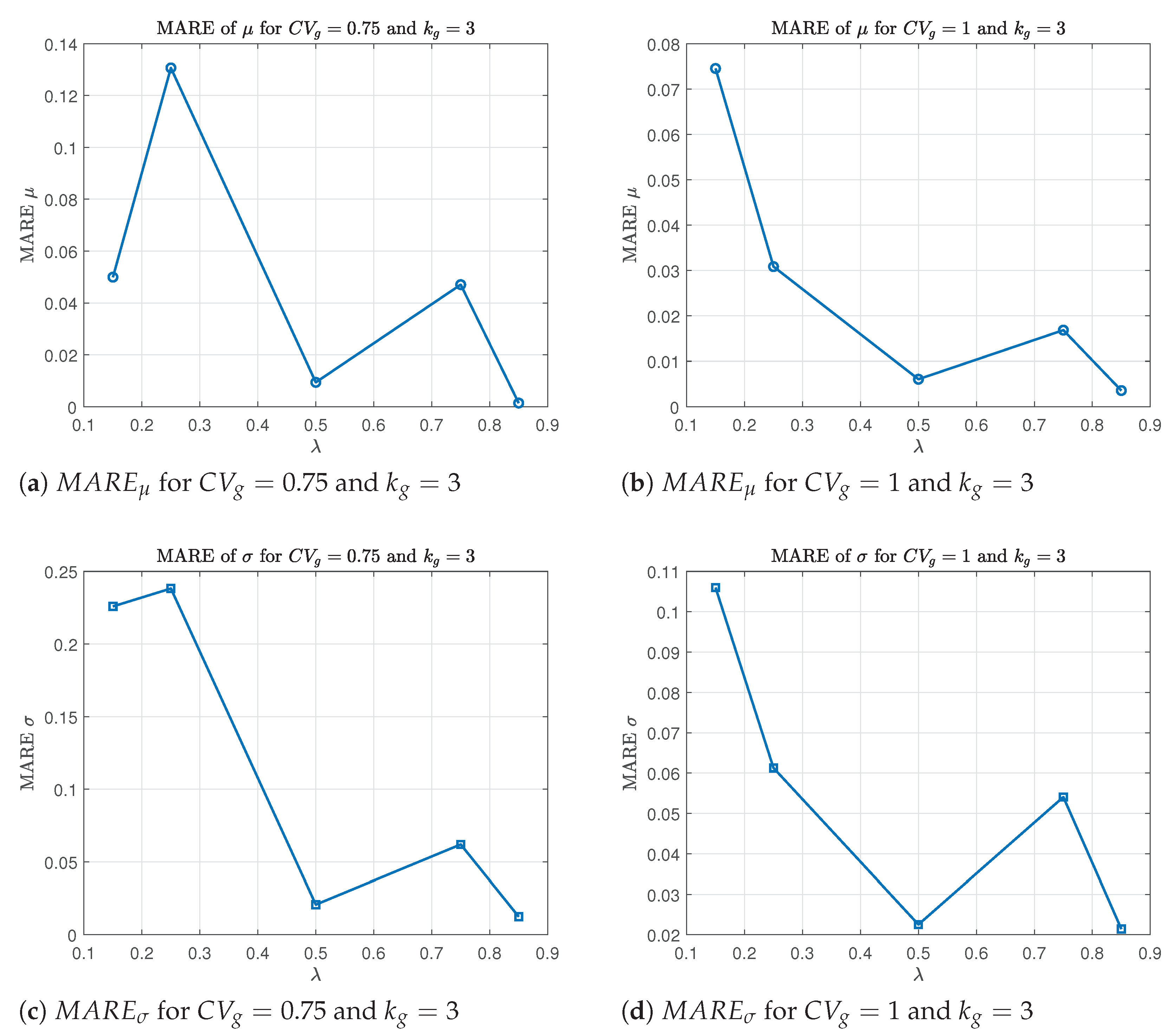
To evaluate how estimation accuracy varies with the parameter values used in the simulations, we analyze the behavior of the estimated parameters , , and as increases from 0.15 to 0.85. For comparison purposes, the coefficient of variation and the shape parameter are held fixed (see Figure 1).
For each pair , we observe a general trend of decreasing relative error in as increases. This is expected, as the same absolute estimation error in corresponds to a smaller relative error when is large. A similar decreasing trend is also observed for the MARE of and , particularly for smaller values of . As increases, the BC transformation becomes smoother and more stable, which improves the performance of the maximum likelihood estimation. The reduction in skewness and better approximation to normality help reduce the variability in estimating and , leading to more accurate and reliable parameter estimates.
Figure 2.
MARE and as a function of fixing the parameters and .
By contrast, the MSE curves for the same estimators and parameter settings (not shown) exhibit irregular behavior, often increasing with when estimator variability outweighs squared bias, which limits the usefulness of MSE for comparative analysis across the PN parameter space. To provide a comprehensive comparison of the two approaches for maximizing the log-likelihood—estimating all three parameters simultaneously or only —we computed the average MB, MSE, and MARE statistics for each parameter across the entire dataset, as summarized in Table 1.
Estimation results depend on the specific values of the underlying parameters. Some methods perform better than others for certain parameter combinations and worse for others. For this reason, we chose to compare the methods based on the overall average of each error statistic. Note that these statistics themselves are computed as averages over multiple simulated datasets for each parameter combination. The results indicate that maximizing the log-likelihood function with all three parameters simultaneously (the mode) yields the best performance overall. In particular, the average MARE for shows an improvement of approximately over the classical estimator and about over the mode. The average mean bias for follows a similar trend as the average MARE, although the differences between methods are more pronounced. As for the average statistics associated with and , we observe that method , implemented via ML in all three parameters, outperforms the version of the approach. Furthermore, method shows a substantial advantage over both and modes of in terms of the average MSE for .
4. Conclusions and Future Work
In this work, we present in detail methods for estimating the parameters of the PN, which has yet to reveal all of its properties. The quality of the results depends not only on the selected parameter values but also on the specific statistic used to evaluate and compare the maximum likelihood estimates. The foundation of our computational approach is the N-R method, which had to be carefully tuned to ensure proper convergence. The estimation process required extensive experimentation to achieve reliable and satisfactory results.
Classical estimation in the PN distribution, as proposed by Box and Cox [9], was primarily intended to achieve approximate normality of the transformed data. However, the inconsistency of those estimators renders them unsuitable when accurate parameter estimation is the objective. Exact ML estimation was studied by Goto et al. [4], although implemented differently from the approach adopted in this work. We implemented both methods using simultaneous ML estimation of all three parameters. The results indicate an improvement in the estimation of over the method, although this improvement is not substantial when compared to the mode. In contrast, for the parameters and , we observe a significant enhancement in estimation accuracy under the method relative to the implementation.
Given its close relation to the BC transformation, the correlation structure of variables on the PN scale remains to be fully understood. Under appropriate parameter settings, independent transformation of the marginal variables result in a bivariate approximated normal pair. Understanding this phenomenon may offer practitioners valuable insights into how transformed data under the Box-Cox framework can be analyzed and interpreted.
Abbreviations
The following abbreviations are used in this manuscript:
| ML | Maximum Likelihood |
| MLE | Maximum Likelihood Estimation |
| MB | Mean Bias |
| MSE | Mean Square Error |
| MARE | Mean Absolute Relative Error |
| N-R | Newton-Raphson |
Appendix A

Table A1.
Parameters and their ML estimates obtained with the method . The last 9 columns are values of the statistics MB, MSE and MARE over the generated data sets for each set of parameters.
Table A1.
Parameters and their ML estimates obtained with the method . The last 9 columns are values of the statistics MB, MSE and MARE over the generated data sets for each set of parameters.
| 0.15 | 0.75 | 3 | 5.3333 | 4.0000 | 0.1896 | 5.5996 | 4.9035 | 0.0396 | 0.2663 | 0.9035 | 0.0360 | 31.3559 | 24.0447 | 0.2640 | 0.0499 | 0.2259 |
| 0.15 | 1.00 | 3 | 3.3333 | 3.3333 | 0.1887 | 3.5818 | 3.6866 | 0.0387 | 0.2484 | 0.3533 | 0.0360 | 12.8796 | 13.6751 | 0.2579 | 0.0745 | 0.1060 |
| 0.15 | 2 | 2 | 2.2222 | 4.4444 | 0.1435 | 2.1539 | 4.3051 | -0.0065 | -0.0683 | -0.1394 | 0.0219 | 4.8608 | 19.0066 | 0.0434 | 0.0307 | 0.0314 |
| 0.15 | 2 | 3 | 1.3333 | 2.6667 | 0.1485 | 1.2989 | 2.6719 | -0.0015 | -0.0345 | 0.0052 | 0.0224 | 1.7172 | 7.1599 | 0.0099 | 0.0258 | 0.0020 |
| 0.15 | 4 | 1 | 2.2222 | 8.8889 | 0.1098 | 3.5788 | 6.8704 | -0.0402 | 1.3566 | -2.0185 | 0.0130 | 12.9494 | 48.1586 | 0.2678 | 0.6105 | 0.2271 |
| 0.15 | 4 | 2 | 0.9524 | 3.8095 | 0.0880 | 1.3445 | 3.3695 | -0.0620 | 0.3921 | -0.4400 | 0.0077 | 1.8076 | 11.3538 | 0.4135 | 0.4117 | 0.1155 |
| 0.15 | 4 | 3 | 0.6061 | 2.4242 | 0.1435 | 0.6111 | 2.4736 | -0.0065 | 0.0051 | 0.0493 | 0.0209 | 0.4083 | 6.1337 | 0.0434 | 0.0083 | 0.0203 |
| 0.15 | 8 | 1 | 0.9524 | 7.6191 | 0.0927 | 2.3671 | 5.4337 | -0.0573 | 1.4147 | -2.1854 | 0.0087 | 5.7301 | 29.6171 | 0.3822 | 1.4855 | 0.2868 |
| 0.15 | 8 | 2 | 0.4444 | 3.5556 | 0.1122 | 0.3315 | 3.3777 | -0.0379 | -0.1130 | -0.1778 | 0.0126 | 0.1230 | 11.4097 | 0.2523 | 0.2542 | 0.0500 |
| 0.15 | 8 | 3 | 0.2899 | 2.3188 | 0.1336 | 0.2200 | 2.3925 | -0.0164 | -0.0698 | 0.0737 | 0.0182 | 0.0772 | 5.7352 | 0.1096 | 0.2409 | 0.0318 |
| 0.25 | 0.75 | 3 | 3.2000 | 2.4000 | 0.3151 | 3.6181 | 2.9717 | 0.0651 | 0.4181 | 0.5717 | 0.1001 | 13.1587 | 8.9682 | 0.2602 | 0.1306 | 0.2382 |
| 0.25 | 1 | 2 | 4.0000 | 4.0000 | 0.2761 | 4.0226 | 4.5401 | 0.0261 | 0.0226 | 0.5401 | 0.0775 | 16.3286 | 21.0141 | 0.1045 | 0.0057 | 0.1350 |
| 0.25 | 1 | 3 | 2.0000 | 2.0000 | 0.2149 | 1.9383 | 1.8775 | -0.0351 | -0.0617 | -0.1225 | 0.0492 | 3.7888 | 3.5605 | 0.1404 | 0.0309 | 0.0613 |
| 0.25 | 2 | 1 | 4.0000 | 8.0000 | 0.2430 | 3.4671 | 7.5425 | -0.0070 | -0.5329 | -0.4575 | 0.0591 | 13.5446 | 57.5633 | 0.0279 | 0.1332 | 0.0572 |
| 0.25 | 2 | 2 | 1.3333 | 2.6667 | 0.1931 | 1.2999 | 2.4774 | -0.0569 | -0.0334 | -0.1892 | 0.0375 | 1.7104 | 6.1448 | 0.2277 | 0.0251 | 0.0710 |
| 0.25 | 2 | 3 | 0.8000 | 1.6000 | 0.2136 | 0.6654 | 1.5492 | -0.0364 | -0.1346 | -0.0508 | 0.0456 | 0.4428 | 2.4001 | 0.1456 | 0.1682 | 0.0317 |
| 0.25 | 4 | 1 | 1.3333 | 5.3333 | 0.1564 | 1.9949 | 3.7137 | -0.0936 | 0.6615 | -1.6197 | 0.0253 | 4.0425 | 13.8868 | 0.3745 | 0.4962 | 0.3037 |
| 0.25 | 4 | 3 | 0.3636 | 1.4546 | 0.2282 | 0.3693 | 1.4822 | -0.0218 | 0.0057 | 0.0276 | 0.0560 | 0.1560 | 2.2080 | 0.0871 | 0.0155 | 0.0190 |
| 0.25 | 8 | 1 | 0.5714 | 4.5714 | 0.1488 | 1.3459 | 3.1108 | -0.1012 | 0.7745 | -1.4606 | 0.0222 | 1.8114 | 9.6770 | 0.4047 | 1.3553 | 0.3195 |
| 0.25 | 8 | 2 | 0.2667 | 2.1333 | 0.1918 | 0.1981 | 2.0368 | -0.0582 | -0.0686 | -0.0966 | 0.0368 | 0.0392 | 4.1485 | 0.2330 | 0.2572 | 0.0453 |
| 0.25 | 8 | 3 | 0.1739 | 1.3913 | 0.2534 | 0.0976 | 1.4223 | 0.0034 | -0.0763 | 0.0310 | 0.0677 | 0.0178 | 2.0308 | 0.0134 | 0.4388 | 0.0223 |
| 0.50 | 0.75 | 2 | 4.0000 | 3.0000 | 0.4091 | 3.5164 | 2.4831 | -0.0909 | -0.4836 | -0.5169 | 0.1683 | 12.4139 | 6.2321 | 0.1818 | 0.1209 | 0.1723 |
| 0.50 | 0.75 | 3 | 1.6000 | 1.2000 | 0.4926 | 1.5850 | 1.2249 | -0.0074 | -0.0150 | 0.0249 | 0.2515 | 2.5284 | 1.5350 | 0.0148 | 0.0094 | 0.0207 |
| 0.50 | 1 | 2 | 2.0000 | 2.0000 | 0.4547 | 1.8994 | 1.9925 | -0.0453 | -0.1006 | -0.0075 | 0.2318 | 3.6422 | 4.3440 | 0.0907 | 0.0503 | 0.0037 |
| 0.50 | 1 | 3 | 1.0000 | 1.0000 | 0.5029 | 1.0060 | 1.0225 | 0.0029 | 0.0060 | 0.0225 | 0.2640 | 1.0213 | 1.0600 | 0.0059 | 0.0060 | 0.0225 |
| 0.50 | 2 | 1 | 2.0000 | 4.0000 | 0.2772 | 2.0979 | 2.3371 | -0.2228 | 0.0979 | -1.6629 | 0.0768 | 4.4012 | 5.4621 | 0.4456 | 0.0490 | 0.4157 |
| 0.50 | 2 | 2 | 0.6667 | 1.3333 | 0.4455 | 0.6325 | 1.2503 | -0.0545 | -0.0342 | -0.0830 | 0.1997 | 0.4124 | 1.5650 | 0.1090 | 0.0513 | 0.0623 |
| 0.50 | 2 | 3 | 0.4000 | 0.8000 | 0.4922 | 0.3976 | 0.7984 | -0.0078 | -0.0024 | -0.0016 | 0.2465 | 0.1613 | 0.6395 | 0.0156 | 0.0060 | 0.0020 |
| 0.50 | 4 | 1 | 0.6667 | 2.6667 | 0.3395 | 1.1489 | 1.9508 | -0.1606 | 0.4823 | -0.7159 | 0.1152 | 1.3201 | 3.8054 | 0.3211 | 0.7234 | 0.2685 |
| 0.50 | 4 | 2 | 0.2857 | 1.1429 | 0.3848 | 0.2396 | 1.0822 | -0.1153 | -0.0461 | -0.0607 | 0.1503 | 0.0641 | 1.1759 | 0.2305 | 0.1615 | 0.0531 |
| 0.50 | 4 | 3 | 0.1818 | 0.7273 | 0.4830 | 0.1762 | 0.7265 | -0.0170 | -0.0056 | -0.0008 | 0.2391 | 0.0348 | 0.5289 | 0.0339 | 0.0308 | 0.0010 |
| 0.50 | 8 | 1 | 0.2857 | 2.2857 | 0.3027 | 0.5169 | 1.9333 | -0.1973 | 0.2311 | -0.3525 | 0.0916 | 0.2671 | 3.7375 | 0.3946 | 0.8090 | 0.1542 |
| 0.50 | 8 | 2 | 0.1333 | 1.0667 | 0.3850 | 0.1022 | 1.0242 | -0.1150 | -0.0311 | -0.0424 | 0.1498 | 0.0144 | 1.0528 | 0.2300 | 0.2334 | 0.0398 |
| 0.50 | 8 | 3 | 0.0870 | 0.6957 | 0.4969 | 0.0815 | 0.6990 | -0.0031 | -0.0055 | 0.0034 | 0.2531 | 0.0096 | 0.4900 | 0.0061 | 0.0632 | 0.0049 |
| 0.75 | 0.75 | 2 | 2.6667 | 2.0000 | 0.7761 | 2.7286 | 2.2088 | 0.0261 | 0.0619 | 0.2088 | 0.6176 | 7.5403 | 5.1149 | 0.0348 | 0.0232 | 0.1044 |
| 0.75 | 0.75 | 3 | 1.0667 | 0.8000 | 0.8324 | 1.1169 | 0.8496 | 0.0824 | 0.0502 | 0.0496 | 0.6990 | 1.2529 | 0.7261 | 0.1098 | 0.0471 | 0.0619 |
| 0.75 | 1 | 2 | 1.3333 | 1.3333 | 0.6969 | 1.2810 | 1.3147 | -0.0532 | -0.0523 | -0.0186 | 0.5102 | 1.6635 | 1.7908 | 0.0709 | 0.0392 | 0.0140 |
| 0.75 | 1 | 3 | 0.6667 | 0.6667 | 0.8108 | 0.6779 | 0.7027 | 0.0608 | 0.0113 | 0.0361 | 0.6686 | 0.4647 | 0.4966 | 0.0811 | 0.0169 | 0.0541 |
| 0.75 | 2 | 1 | 1.3333 | 2.6667 | 0.5901 | 1.5127 | 2.1045 | -0.1599 | 0.1794 | -0.5622 | 0.3868 | 2.3117 | 4.9215 | 0.2132 | 0.1345 | 0.2108 |
| 0.75 | 2 | 2 | 0.4444 | 0.8889 | 0.6820 | 0.4419 | 0.8564 | -0.0680 | -0.0026 | -0.0325 | 0.4839 | 0.1998 | 0.7403 | 0.0906 | 0.0057 | 0.0366 |
| 0.75 | 2 | 3 | 0.2667 | 0.5333 | 0.8019 | 0.2615 | 0.5534 | 0.0519 | -0.0052 | 0.0201 | 0.6585 | 0.0703 | 0.3073 | 0.0691 | 0.0196 | 0.0377 |
| 0.75 | 4 | 1 | 0.4444 | 1.7778 | 0.4901 | 0.6700 | 1.2703 | -0.2599 | 0.2256 | -0.5075 | 0.2504 | 0.4616 | 1.6468 | 0.3465 | 0.5075 | 0.2854 |
| 0.75 | 4 | 2 | 0.1905 | 0.7619 | 0.6639 | 0.1790 | 0.7356 | -0.0861 | -0.0115 | -0.0263 | 0.4590 | 0.0357 | 0.5438 | 0.1148 | 0.0603 | 0.0345 |
| 0.75 | 4 | 3 | 0.1212 | 0.4849 | 0.8179 | 0.1235 | 0.4942 | 0.0679 | 0.0023 | 0.0094 | 0.6770 | 0.0168 | 0.2451 | 0.0905 | 0.0190 | 0.0194 |
| 0.75 | 8 | 1 | 0.1905 | 1.5238 | 0.4044 | 0.3496 | 1.0833 | -0.3456 | 0.1591 | -0.4405 | 0.1663 | 0.1338 | 1.1811 | 0.4608 | 0.8352 | 0.2891 |
| 0.75 | 8 | 2 | 0.0889 | 0.7111 | 0.6310 | 0.0813 | 0.6856 | -0.1190 | -0.0076 | -0.0255 | 0.4097 | 0.0095 | 0.4720 | 0.1586 | 0.0850 | 0.0359 |
| 0.75 | 8 | 3 | 0.0580 | 0.4638 | 0.8221 | 0.0655 | 0.4720 | 0.0721 | 0.0075 | 0.0082 | 0.6839 | 0.0054 | 0.2235 | 0.0961 | 0.1295 | 0.0178 |
| 0.85 | 0.75 | 2 | 2.3529 | 1.7647 | 0.8252 | 2.3113 | 1.7627 | -0.0248 | -0.0417 | -0.0021 | 0.6964 | 5.4118 | 3.2031 | 0.0292 | 0.0177 | 0.0012 |
| 0.85 | 0.75 | 3 | 0.9412 | 0.7059 | 0.8364 | 0.9399 | 0.6971 | -0.0136 | -0.0013 | -0.0088 | 0.7068 | 0.8875 | 0.4891 | 0.0160 | 0.0014 | 0.0125 |
| 0.85 | 1 | 2 | 1.1765 | 1.1765 | 0.8498 | 1.1609 | 1.1978 | -0.0003 | -0.0156 | 0.0213 | 0.7302 | 1.3598 | 1.4557 | 0.0003 | 0.0133 | 0.0181 |
| 0.85 | 1 | 3 | 0.5882 | 0.5882 | 0.8611 | 0.5903 | 0.6009 | 0.0111 | 0.0021 | 0.0126 | 0.7460 | 0.3507 | 0.3622 | 0.0130 | 0.0036 | 0.0214 |
| 0.85 | 2 | 1 | 1.1765 | 2.3529 | 0.7305 | 1.3838 | 1.9647 | -0.1195 | 0.2073 | -0.3883 | 0.5618 | 1.9442 | 4.0743 | 0.1406 | 0.1762 | 0.1650 |
| 0.85 | 2 | 2 | 0.3922 | 0.7843 | 0.7744 | 0.3813 | 0.7633 | -0.0757 | -0.0108 | -0.0211 | 0.6194 | 0.1499 | 0.5864 | 0.0890 | 0.0277 | 0.0269 |
| 0.85 | 2 | 3 | 0.2353 | 0.4706 | 0.8898 | 0.2380 | 0.4815 | 0.0398 | 0.0027 | 0.0109 | 0.7950 | 0.0577 | 0.2324 | 0.0468 | 0.0114 | 0.0232 |
| 0.85 | 4 | 1 | 0.3922 | 1.5686 | 0.5718 | 0.5819 | 1.1426 | -0.2782 | 0.1897 | -0.4260 | 0.3521 | 0.3539 | 1.3327 | 0.3273 | 0.4837 | 0.2716 |
| 0.85 | 4 | 2 | 0.1681 | 0.6723 | 0.7624 | 0.1588 | 0.6554 | -0.0876 | -0.0093 | -0.0169 | 0.5946 | 0.0277 | 0.4312 | 0.1030 | 0.0552 | 0.0252 |
| 0.85 | 4 | 3 | 0.1070 | 0.4278 | 0.8820 | 0.1077 | 0.4307 | 0.0320 | 0.0008 | 0.0029 | 0.7826 | 0.0124 | 0.1861 | 0.0377 | 0.0072 | 0.0068 |
| 0.85 | 8 | 1 | 0.1681 | 1.3445 | 0.5304 | 0.3287 | 0.9851 | -0.3196 | 0.1607 | -0.3594 | 0.3200 | 0.1176 | 0.9876 | 0.3760 | 0.9559 | 0.2673 |
| 0.85 | 8 | 2 | 0.0784 | 0.6275 | 0.7356 | 0.0688 | 0.6116 | -0.1144 | -0.0097 | -0.0158 | 0.5531 | 0.0069 | 0.3752 | 0.1346 | 0.1230 | 0.0252 |
| 0.85 | 8 | 3 | 0.0512 | 0.4092 | 0.8593 | 0.0515 | 0.4112 | 0.0093 | 0.0004 | 0.0020 | 0.7436 | 0.0038 | 0.1696 | 0.0109 | 0.0076 | 0.0049 |
References
- Gonçalves, R. The power-normal distribution. AIP Conf. Proc. 2019, 2116, 110009. [Google Scholar] [CrossRef]
- Gonçalves, R. The power-normal distribution. J. Phys.: Conf. Ser. 2019, 1334, 012014. [Google Scholar] [CrossRef]
- Gonçalves, R. Exact vs Approximated ML Estimation for the Box-Cox Transformation. AIP Conf. Proc. 2024, 3094, 500034. [Google Scholar] [CrossRef]
- Goto, M.; Inoue, T.; Tsuchya, Y. On the Estimation of Parameters in the Power-Normal Distribution. Bull. Inf. Cybern. 1984, 21, 41–53. [Google Scholar]
- Atkinson, A.; Pericchi, L.; Smith, R. Grouped Likelihood for the Shifted Power Transformation. J. R. Stat. Soc. Ser. B 1991, 39, 473–482. [Google Scholar] [CrossRef]
- Gnanadesikan, R. Methods for Statistical Data Analysis of Multivariate Observations; John Wiley & Sons: New York, NY, USA, 1977; ISBN 978-0-471-30845-4. [Google Scholar]
- Barr, D.; Sherrill, T. Mean and Variance of Truncated Normal Distributions. Am. Stat. 1999, 53, 357–361. [Google Scholar] [CrossRef]
- Goto, M.; Inoue, T. Some Properties of the Power-Normal Distribution. J. Biometrics 1980, 1, 28–54. [Google Scholar] [CrossRef]
- Box, G.E.; Cox, D.R. An Analysis of Transformations. J. R. Stat. Soc. Ser. B 1964, 26, 211–243. [Google Scholar] [CrossRef]
- Freeman, J.; Modarres, R. Inverse Box-Cox: The Power-Normal Distribution. Stat. Probab. Lett. 2006, 1, 764–772. [Google Scholar] [CrossRef]
- Gonçalves, R. Inverse Box-Cox and the Power-Normal Distribution. In Innovation, Engineering and Entrepreneurship; Lecture Notes in Electrical Engineering; Springer: Cham, Switzerland, 2019; Volume 505, pp. 805–810. [Google Scholar]
- Johnson, N.L.; Kotz, S.; Balakrishnan, N. Continuous Univariate Distributions, Volume 1, 2nd ed.; Wiley: New York, NY, USA, 1994. [Google Scholar]
- Cohen, A.C. Estimation in the truncated normal distribution. J. Am. Stat. Assoc. 1950, 45, 290–299. [Google Scholar]
Figure 1.
MARE of as a function of fixing the parameters and .
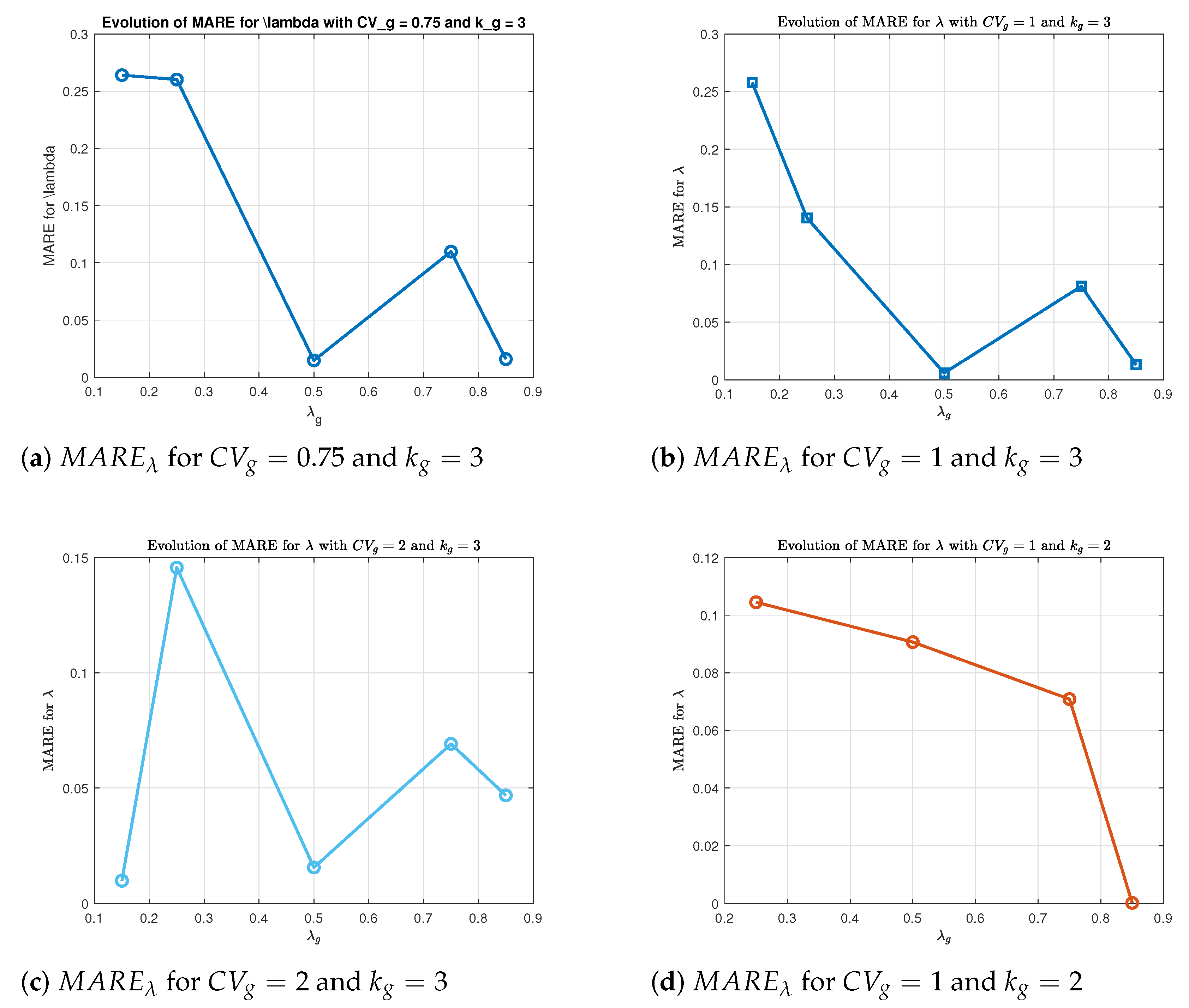
Table 1.
Summary statistics for MB, MSE and MARE for the parameters under different estimation methods.
Table 1.
Summary statistics for MB, MSE and MARE for the parameters under different estimation methods.
| Method | MB | MB | MB | MSE | MSE | MSE | MARE | MARE | MARE |
|---|---|---|---|---|---|---|---|---|---|
Note: MB = Mean Bias; MSE = Mean Squared Error; MARE = Mean Absolute Relative Error.
Disclaimer/Publisher’s Note: The statements, opinions and data contained in all publications are solely those of the individual author(s) and contributor(s) and not of MDPI and/or the editor(s). MDPI and/or the editor(s) disclaim responsibility for any injury to people or property resulting from any ideas, methods, instructions or products referred to in the content. |
© 2025 by the authors. Licensee MDPI, Basel, Switzerland. This article is an open access article distributed under the terms and conditions of the Creative Commons Attribution (CC BY) license (http://creativecommons.org/licenses/by/4.0/).
Copyright: This open access article is published under a Creative Commons CC BY 4.0 license, which permit the free download, distribution, and reuse, provided that the author and preprint are cited in any reuse.


