
Submitted:
04 June 2024
Posted:
05 June 2024
You are already at the latest version
Abstract
This manuscript presents a new two-parameter unit stochastic distribution, obtained by transforming the Laplace distribution, using generalized logistic map, into a unit interval. The distribution thus obtained is named the Laplace-logistic unit (abbreviated LLU) distribution, and its basic stochastic properties are examined in detail. Also, the procedure for estimating parameters based on quantiles is provided, along with the asymptotic properties of the obtained estimates and the appropriate numerical simulation study. Finally, the application of the LLU distribution in dynamic and regression analysis of real-world data with accentuated "peaks" and "fat" tails is also discussed.
Keywords:
unit distributions
; Laplace distribution
; generalized logistic map
; stochastic properties
; parameter estimation
; quantiles
; dynamics
; regression
MSC: 60E05; 62E10; 62F10
1. Introduction
Unit stochastic distributions, defined on the interval , represent an important tool of contemporary probability theory. They are primarily used as stochastic models that can describe so-called proportional (percentage) variables and represent theoretical models that can successfully explain the behaviour of some real-world phenomena (see, as more contemporary, e.g. [1,2,3,4,5,6,7,8,9,10,11,12,13]). On the other hand, modeling with unit distributions differs from common stochastic modeling procedures, primarily due to the limitation of data within interval. Although the procedure for creating unit distributions can be given in a general form [14], the most common approach is based on continuous transformations of distributions defined on infinite intervals into a unit interval (as some recent results, see e.g. [15,16,17,18,19,20,21,22,23]). Nevertheless, most of these distributions are limited by a unique form of (a)symmetry and modality, "vanishing" data at the ends of the unit interval, etc. This is often inappropriate for modeling real phenomena with different characteristics, especially where data with pronounced "peaks" and "fat tails" appear.
To this end, proceeding from similar considerations as in Stojanović et al. [24], Stojanović et al. [25], a new unit distribution, named the Laplace-logistic unit (LLU) distribution, is described here. It is based on a general logistic mapping of the Laplace distribution to a unit interval, and as will be seen, has considerable flexibility and suitability for describing a variety of empirical distributions, from those with pronounced extremes to increasing, decreasing or bathtub-shaped ones. The definition and the key stochastic properties of the LLU distribution, regarding its limit properties, (a)symmetry and modality, are presented in the next Section 2. Thereafter, Section 3 considers the parameters estimation based on sample quantiles, the asymptotic properties of thus obtained estimators, as well as their numerical Monte Carlo study. An application of the LLU distribution in fitting some real-world data, primarily from the aspect of dynamic and regression analysis, is presented in Section 4, while Section 5 contains some concluding remarks.
2. The LLU Distribution
2.1. Definition and Main Properties
Let us first consider a random variable (RV) Y with a symmetric Laplace distribution, whose probability density function (PDF) is:
where and is the scale parameter. For an arbitrary , let us define the so-called general logistic map , which is the bijective, continuous transformation , with limits:
Using Equation (1) and the inverse transformation , the new RV , defined on the unit interval is obtained. After some computation, for the PDF of the RV X one obtains:
where and . Thus, we say that the RV X, whose PDF is given by Equation (2), has a Laplace-logistic unit (LLU) distribution, with the parameters , or abbr. . Obviously, LLU distribution is a two-parameter distribution, where, in addition to the scale parameter , there is also a shape parameter . Also, let us emphasize that symmetric Laplace density is expressed in terms of the absolute difference from the zero and it has pronounced “peaks” and tails more "fat" than, for instance, the Gaussian distribution. For these reasons, the RV will have similar properties, but it also has some other specificities. To describe them more completely, we first introduce some terms related to the limit behaviour of the density at the ends of the unit interval:
Definition 1.
Let be the RV with the LLU distribution, whose PDF is given by Equation (2). The PDF is left-(right-)vanishing if is valid:
Otherwise, the PDF is left-(right-)tailed.
Now, some properties of the LLU distribution regarding its possible shapes and boundary characteristics can be given by the following proposition:
Theorem 1.
The PDF of the RV is continuous function, non-differentiable at the point , with the following properties:
- When and , it is decreasing.
- When and , it is increasing.
- When , and , it is left-tailed and right-vanishing.
- When , and , it is right-tailed and left-vanishing.
- When and , it is (both sides) tailed.
- When and , it is (both sides) vanishing.
Proof.
For simplicity, let us denote the left and right branches of the PDF , respectively, as follows:
Accordingly, it is obtained:
so the PDF is indeed continuous at . Furthermore, after some computation, one obtains:
as well as:
Thus, the sign of the partial derivatives in Equation (4) depends on the sign of the functions:
Obviously, both of these functions are monotonically increasing on , and their values at the critical points are, respectively,
Then, by using Equations (3) and (5), all cases in the statement of the theorem are simply obtained. □
Remark 1.
The different conditions for the shape and boundary behavior of the LLU distribution can be seen in Figure 1 (a), where the six different areas mentioned in the previous Theorem are shown. On the other hand, Figure 1 (b) shows typical, different shapes of the PDFs of this distribution. As can be easily seen, the LLU distribution takes very different forms, where in addition to the typical one with a "peak", which is similar to the Laplace distribution, it can have a decreasing, increasing or bathtub-shaped PDF. In that way, it has a significant flexibility, which is of particular importance in applications. Moreover, when one obtains:
so in this asymptotic case the PDF will be an approximately differentiable, with extreme value (i.e. mode) at the point . In any case, the modality of the LLU distribution will be explored in more detail in the next part of this section.
The PDF of the LLU distribution can also be used to obtain its moments and other moment-based features, as given below.
Theorem 2.
The moment of the LLU of the distributed RV X can be expressed as:
where r is an integer and is an incomplete beta function. In addition, the following convergence holds:
Proof.
Remark 2.
By using Equation (6), for the mean and the variance of the RV ones obtain, respectively,
Additionally, according to Equation (7), it follows:
that is, in this limit case, holds, where "as" means "almost surely". Therefore, the RV X is then reduced to a unit constant, obtained by transforming the Laplace distribution, whose PDF is given by Equation (1), using the trivial logistic map . This can also be seen in Figure 2 below, where 3D plots of mean value and variance are shown, depending on the parameters .
Similarly, the skewness coefficient and the kurtosis of the RV are, respectively,
Nevertheless, because of the complexity though, a more detailed procedure for calculating these coefficients will be omitted.
2.2. Cumulative, Hazard and Quantile Function
Using Equation (2), the cumulative distribution function (CDF) of the LLU distribution can be obtained as follows:
where . Note that the function is differentiable on , and well defined outside the unit interval, since it is valid:
Furthermore, according to Equations (2) and (8), the hazard rate function (HRF) can be obtained as follows:
The basic properties of the HRF can be expressed by the following statement:
Theorem 3.
Let and is the HRF of the RV X, defined by Equation (10). Then, is a continuous function, non-differentiable at the point , with the following properties:
- When and , it is (both sides) tailed with a local maxima at .
- When and , it is (both sides) tailed without maxima, that is, bathtub-shaped.
- When and , it is left-vanishing with a local maxima at .
- When and , it is increasing.
Proof.
Remark 3.
Plots of the CDF and HRF of the LLU distribution are given in Figure 3 below. It is known that the hazard (failure) rate represents the failure frequency of the designed system or component. Thus, the HRF usually increases, which means that the probability that the designed system or component will fail increases. In contrary, decreasing failure rate (DFR) describes the phenomenon where this probability decreases in some interval. As can be concluded from the previous theorem, both of these situations can be obtained from the LLU distribution, for certain values of its parameters. Moreover, in cases where HRF has a local maximum at , the "peaked" value can then be interpreted as the critical point of the system. Therefore, these properties of HRF give diverse possibilities of its practical application, which will be discussed later.
In the last part of this section, the so-called quantile function (QF) of the LLU distribution is considered, obtained as inverse function of its CDF:
where . The QF is a useful tool for obtaining some other properties of the LLU distribution, primarily related to its modality and (a)symmetry.
Theorem 4.
Let be the LLU distributed RV, whose QF is given by Equation (13). Then, the following statements hold:
- The RV X is symmetrically distributed if and only if . Otherwise, X is positively asymmetric when , and negatively asymmetric when .
- The RV X is unimodal, with the mode , if and only if and .
Proof. By substituting the quantile in the QF , it is obtained the median . Thus, the RV X is symmetrically distributed if and only if the median is equal to 1/2, that is, when . The positive and negative asymmetry conditions are also easily obtained, by solving the inequalities and , respectively.
Using the rule for the derivative of the inverse function, for the derivatives up to the second order of the QF one obtains:
where . Further, if we denote:
then, after some computation, it is obtained:
Obviously, the sign of derivatives in Equation (15) depends on the sign of the functions:
which are, respectively, monotonically decreasing and increasing on . Thus, according to the second one in Equations (14), the RV X has a local maxima at if and only if the following inequalities hold:
Therefore, Equations (16) obviously provide a statement of this part of the theorem. □
Remark 4.
Theorem 4, along with the previously proved Theorem 1, give a complete insight into the variety of shapes of the LLU distribution (see again Figure 1). At the same time, note that its median and mode are equal, but that the true symmetry holds only for . This can also be confirmed by the definition of the PDF of LLU distribution, given by Equation (2), based on which it follows for each .
Remark 5.
Using the QF , given by Equation (13), some more measures of shape of the CLU distribution can be studied. These are, for instance, Galton’s skewness (GS) which measures the degree of long tail, and Moors kurtosis (MK) which measures the degree of weight of the tail of the distribution (see, e.g. [12]). In the case of the LLU distribution, these two measures, after some calculation, can be expressed as:
and 3D plots of their dependence in relation to are given in Figure 4.
3. Parameters Estimation & Simulation Study
In this section, the procedure for estimating the unknown parameters of the LLU-distributed RV X is presented. In doing so, note that according to the previously described properties of the LLU distribution, using some common procedures to estimate its parameters has some difficulties. Thus, for instance, due to the fact that the moments of the LLU distribution, given by Equation (6), are expressed using the beta function, the method of moments requires certain complex calculations. On the other hand, since the PDF of the LLU distribution is not a differentiable at , the usage of the maximum likelihood (ML) estimation method is very specific. Considering that the ML estimator of the scale parameter in the case of the Laplace distribution is equal to the sample median (see, for more detail Norton [26]), here we consider methods of parameter estimation based on the quantiles of the LLU distribution.
For that cause, let be the random sample of the length n, for which we define the corresponding order statistics . As is well-known, PDF of i-th order statistics is given as follows:
where . By substituting , into the QF , given by Equation (13), for the quartiles of the RV X one obtains:
while the second quartile is the median . On the other hand, the sample quantiles are given by equality:
where is the integer part of . In this way, the sample quantiles are in fact the order statistics, and their distribution can be obtained according to Equation (17).
Furthermore, the sample quartiles , can be used as the estimators of theoretical ones. Thus, by equating median of the RV X with the sample one , the estimator of the shape parameter is easily obtained. In addition, according to Equations (18) it follows:
and using the estimator , for the estimator of the scale parameter one obtains:
In the following, we examine the asymptotic properties of the proposed estimators:
Theorem 5.
Statistics are consistent and asymptotic normal (AN) estimators of the true parameters , respectively.
Proof.
First, by using some general asymptotic sample quantile theory [27], we shall prove the consistency of the proposed estimators. For that cause, let us notice that the CDF is a differentiable and increasing on . Thus, the quantiles are uniquely determined by Equation (13), and sample quantiles are uniquely determined by Equation (19). Using Bahadur’s representation of sample quantiles (see, e.g. Theorem 1 in Dudek Kuczmaszewska [28], or Serfling [29], pp. 91-92), one obtains:
where is the empirical CDF. As is known, for each , the empirical CDF almost surely and uniformly converge to the CDF , when . So, by applying this convergence on Equation (21), when , it follows:
i.e. the sample quantiles are consistent estimators of the theoretical ones. Finally, as estimators are continuous functions of sample quartiles , , by using the property of continuity of almost sure convergence (see, e.g. Serfling [29], pp. 24), it is obtained:
For the proof of the AN property, notice that under the same assumptions sa above, Equation (21) gives the following convergence in distribution:
According to Equation (22), for the sample median one obtains:
wherein is:
Now, using the continuity of convergence in distribution (see, e.g. Serfling [29], pp. 118), for the estimator is obtained:
wherein is:
The AN property of the estimator , given by Equation (20), is similarly proven. For this purpose, let us first define a statistic:
which is consistent estimator of . Using Equation (22), as well as the continuity of convergence in distribution, it follows:
where, after some computations, one obtains:
Finally, according to and Equation (24), it is obtained:
wherein is:
Thus proven convergences in Equations (23) and (25) confirm the AN properties of both proposed estimators . □
Remark 6.
It is worth noting that the variance of the estimator , given by Equation (26), does not depend on the parameter θ. This, among others, is one of the reasons that justifies the use of this estimator.
A numerical study of the effectiveness of the proposed estimators is presented below, based on Monte Carlo simulations of samples taken from the LLU distribution. More precisely, for different samples and parameters values, the proposed estimators were calculated and their statistical analysis was performed. To this end, three different types of samples are considered (see also Figure 5 below):
Sample I is drawn from an increasing LLU distribution with parameters and .
Sample II was drawn from a symmetric, both-sides tailed (i.e. bathtub-shaped) LLU distribution with parameters and .
Sample III was drawn from a symmetric, both-sides vanishing, unimodal LLU distribution with parameters and .
The simulated values of all samples are generated by the R-package "distr" [30], according to which the estimates and are calculated. In order to additionally check the effectiveness of the proposed estimators, the sample realizations of different lengths were observed. It is worth noting that the above sample sizes were chosen similar to some of the real-world data which will be further analyzed. Additionally, independent simulations were performed for each sample, and the results of their statistical analysis are presented in the following Table 1, Table 2 and Table 3.
More precisely, Table 1, Table 2 and Table 3 contain the summary statistics of the obtained estimates, that is, their minimums (Min.), mean values (Mean), maximums (Max.) and standard deviations (SD). Additionally, mean square estimation errors (MSEE), fractional estimation errors (FEE), and the Anderson-Darling (AD) normality test statistics are provided, too. According to this, it can be observed that the proposed estimators are efficient, as the bias, sample range (Max.–Min.), as well as SD and MSEE values decrease with increasing sample size. Thereby, it can be noticed that the estimates are more stable and efficient than . This is due to the fact that the estimate is obtained by a two-step procedure, according to the previously calculated values of , and then using Equation (20).
Similar conclusions can be confirmed based on the AN analysis of the obtained estimates. Its examination was performed using the Anderson-Darling normality test, whose test statistic (AD) and corresponding p-values are calculated using the R-package "nortest" [31]. According to thus obtained results, also presented in Table 1, Table 2 and Table 3, it can be noted that estimates of from smaller samples have a less pronounced AN feature than . Nevertheless, the AN property was confirmed in most cases, especially for larger samples. Some confirmation of these facts can be seen in Figure 5, where realizations, empirical and theoretical distributions of the observed samples are shown.
4. Applications of the LLU distribution
This section discusses some possibilities of applying the LLU distribution in real-world data modeling, primarily in the domain of dynamic and regression analysis. Also, a comparison of the LLU distribution with some existing, well-known and frequently used unit distributions is made. For this purpose, three sets of data are considered, and their brief description is as follows:
The first data set, called Series A, represents broadband usage in rural counties in the United States, based on Microsoft’s Air Belt initiative to help close the rural broadband gap and improve the performance and security of broadband software and services. More specifically, this dataset, taken from the GitHub, Inc. database [32], consists of the percentage of devices connected to the Internet at broadband speed by each zip code, during October 2020.
The second one (Series B), taken from the official website of the National Center for Environmental Information, contains historical data on the melting rate of the South Greenland ice core. The dataset itself was based on research and reconstruction of ice melting rates conducted by Kameda et al. [33] and the World Data Center for Paleoclimatology. In this way, a time series of annual percentage data was generated in the period from 1546. to 1989., the length of which is .
Finally, the third, Series C, is obtained according to the official data from the National Association of Securities Dealers Automated Quotations (NASDAQ) Stock Market [34], and the so-called log-returns of daily changes of natural gas prices (in US dollars per cubic meter), from 1 January, 2018. until to 1 March, 2023. It represents a time series of length , which was also considered in Stojanović et al. [35], where it was shown that it can be viewed as a series of independent realizations of RVs with Laplace distribution. Therefore, this series was transformed using the previously mentioned logistic function and thus is obtained a corresponding regression model with an output variable that can be seen as the realization of independent RVs with LLU distribution.
In order to additionally verify the efficiency of the LLU distribution, it is compared with the well-known Beta distribution and the Kumaraswamy distribution, whose PDFs are, respectively,
Herein is , while are the distribution parameters, and is the beta function. To obtain the estimated values of the parameters of the Beta distribution, the method of moments (MM) is applied, according to which the estimates are as follows:
Here, and are the sample mean and variance, respectively, wherein is . On the other hand, for the Kumaraswamy distribution, the maximum likelihood (ML) estimation method is used, according to which the following parameter estimates are simply obtained (see, e.g. Jones [36]):
We emphasize that one of the reasons for the choice of estimation methods of these two distributions is the comparison not only with their distributions, but also with regard to different estimation procedures.
Realizations of the series mentioned above, along with the fitted PDFs obtained by the previously described estimation procedures, are shown in Figure 6. As can be seen, all series have pronounced and persistent fluctuations, which create "heavy tails" in their distributions. Specifically, Series A has an increasing PDF, for Series B the PDF is positively asymmetric and unimodal, while the PDF of Series C indicates the symmetry of its distribution. Estimated parameter values for each series and for all competing models are shown in Table 4, and independent Monte Carlo simulations were conducted using them. Thereafter, the agreement of the distributions between the actual and fitted data was checked using the MSEE error statistic, the Akaike information criterion (AIC ), and the Kolmogorov- Smirnov (KS) test of equivalence of the asymptotic distribution of two samples. Based on the results thus obtained, it is noticeable that MSEE and AIC values are generally lower when LLU and Beta distribution are applied as the appropriate fitting model. At the same time, it is obvious that the LLU distribution has better fit-characteristics than both other distributions. Moreover, only in the case of the LLU distribution the KS test do not reject, with a significant level , the hypothesis of equivalence with the observed empirical distributions.
5. Conclusion
A new, the so-called the LLU distribution is presented here, along with the corresponding key properties and a procedure for estimating its parameters based on quantiles. The consistency and AN property of the estimators were also examined, as well as a Monte-Carlo study of their efficiency. Finally, a practical application of the LLU distribution in fitting real-world data is presented. To verify the effectiveness of the proposed model, it was applied to fit the distributions of three real-world datasets and compared with the Beta and Kumaraswamy distributions. According to the results obtained in this way, the LLU distribution provides a better fit to the observed data, which is a motivation for further research of some other new unit distributions, with slightly different characteristics. Thus, for instance, by applying the logistic map to some other probability distribution supported on the entire real line (such as, for example, normal, Student or Gumbel distribution), new unit distributions can be obtained and this can be a guideline for some potential further researches for the authors.
Author Contributions
Conceptualization, V.S. and T.J.S.; methodology, V.S. and T.J.S.; software, V.S. and M.J.; validation, V.S., T.J.S. and M.J.; formal analysis, V.S. and T.J.S.; data curation, V.S. and M.J.; writing—original draft preparation, V.S., T.J.S. and M.J.; writing—review and editing, T.J.S. and M.J.; visualization, V.S. and M.J.; supervision, V.S. and T.J.S.; project administration, T.J.S. and M.J. All authors have read and agreed to the published version of the manuscript.
Conflicts of Interest
The authors declare no conflict of interest.
References
- Nakamura, L.R.; Cerqueira, P.H.R.; Ramires, T.G.; Pescim, R.R.; Rigby, R.A.; Stasinopoulos, D.M. A New Continuous Distribution on the Unit Interval Applied to Modelling the Points Ratio of Football Teams. J. Appl. Stat. 2019, 46, 416–431. [CrossRef]
- Hussain, T.; Bakouch, H.S.; Chesneau, C. A New Probability Model With Application to Heavy-Tailed Hydrological Data. Environ. Ecol. Stat. 2019, 26, 127–151. [CrossRef]
- Ghitany, M. E.; Mazucheli, J.; Menezes, A. F. B.; Alqallaf, F. The Unit-Inverse Gaussian Distribution: A New Alternative to Two-Parameter Distributions on the Unit Interval. Commun. Stat. - Theory Methods, 2019, 48, 3423–3438. [CrossRef]
- Mazucheli, J.; Menezes, A. F.; Dey, S. Unit-Gompertz Distribution with Applications. Statistica, 2019a, 79(1), 25–-43. [CrossRef]
- Mazucheli, J.; Menezes, A. F. B.; Chakraborty, S. On the One Parameter Unit-Lindley Distribution and Its Associated Regression Model for Proportion Data. J. Appl. Stat. 2019b, 46(4), 700–714. [CrossRef]
- Gündüz, S.; Mustafa Ç.; Korkmaz, M.C. A New Unit Distribution Based on the Unbounded Johnson Distribution Rule: The Unit Johnson SU Distribution. Pak. J. Stat. Oper. Res. 2020, 16(3), 471–490.
- Afify, A.Z.; Nassar, M., Kumar, D.; Cordeiro, G.M. A New Unit Distribution: Properties and Applications. Electron. J. Appl. Stat. 2022, 15, 460–484.
- Krishna, A.; Maya, R.; Chesneau, C.; Irshad, M.R. The Unit Teissier Distribution and Its Applications. Math. Comput. Appl. 2022, 27(1), 12. [CrossRef]
- Bakouch, H.S.; Hussain, T. ; Tošić, M.; Stojanović, V.S.; Qarmalah, N., Unit Exponential Probability Distribution: Characterization and Applications in Environmental and Engineering Data Modeling, Mathematics 2023, 11(19), Article No. 4207. [CrossRef]
- Korkmaz, M. Ç.; Korkmaz, Z. S. The Unit Log–log Distribution: A New Unit Distribution With Alternative Quantile Regression Modeling and Educational Measurements Applications. J. Appl. Stat. 2023, 50(4), 889–908. [CrossRef]
- Nasiru, S.; Abubakari, A.G.; Chesneau, C. New Lifetime Distribution for Modeling Data on the Unit Interval: Properties, Applications and Quantile Regression. Math. Comput. Appl. 2022, 27, Article No. 105. [CrossRef]
- Nasiru, S.; Abubakari, A.G.; Chesneau, C. The Arctan Power Distribution: Properties, Quantile and Modal Regressions with Applications to Biomedical Data. Math. Comput. Appl. 2023, 28, Article No. 25. [CrossRef]
- Fayomi, A.; Hassan, A.S.; Baaqeel, H.; Almetwally, E.M. Bayesian Inference and Data Analysis of the Unit–Power Burr X Distribution. Axioms 2023, 12, Article No. 297. [CrossRef]
- Condino, F.; Domma, F.; Unit Distributions: A General Framework, Some Special Cases, and the Regression Unit-Dagum Models. Mathematics 2023, 11(13), Article No. 2888. [CrossRef]
- Mazucheli, J.; Menezes, A.F.B.; Fernandes, L.B.; de Oliveira, R.P.; Ghitany, M. E. The Unit-Weibull Distribution as an Alternative to the Kumaraswamy Distribution for the Modeling of Quantiles Conditional on Covariates. J. Appl. Stat. 2019c, 47(6), 954-974. [CrossRef]
- Altun, E. The Log-Weighted Exponential Regression Model: Alternative to the Beta Regression Model. Commun. Stat. - Theory and Methods, 2020, 50(10), 2306–2321. [CrossRef]
- Altun, E.; Cordeiro, G.M. The Unit-Improved Second-Degree Lindley Distribution: Inference and Regression Modeling. Comput. Stat. 2020 35, 259–279. [CrossRef]
- Mazucheli, J.; Bapat, S.R.; Menezes, A.F. A New One-Parameter Unit-Lindley Distribution. Chilean J. Stat. 2020, 11(1), 53–67.
- Krishna, A.; Maya, R.; Chesneau, C.; Irshad, M.R. The Unit Teissier Distribution and Its Applications. Math. Comput. Appl. 2022, 27, Article No. 12. [CrossRef]
- Mustafa, Ç.; Korkmaz, Z; Korkmaz, S. The Unit Log–log Distribution: A New Unit Distribution With Alternative Quantile Regression Modeling and Educational Measurements Applications, J. Appl. Stat. 2023, 50(4), 889–908. [CrossRef]
- Biçer, C.; Bakouch, H.S.; Biçer, H.D.; Alomair, G.; Hussain, T.; Almohisen, A. Unit Maxwell-Boltzmann Distribution and Its Application to Concentrations Pollutant Data. Axioms 2024, 13(4), Article No. 226. [CrossRef]
- Nasiru, S. ; Chesneau, C.; Ocloo, S.K., The Log-Cosine-Power Unit Distribution: A New Unit Distribution for Proportion Data Analysis. Decis. Anal. J. 2024, 10, Article No. 100397. [CrossRef]
- Alsadat, N.; Taniş, C.; Sapkota, L.P.; Kumar, A.; Marzouk, W.; Gemeay, A.M. Inverse unit exponential probability distribution: Classical and Bayesian inference with applications. AIP Advances 2024, 14, Article No. 055108. [CrossRef]
- Stojanović, V.S.; Bojičić, R.; Pažun, B.; Langović, Z. Quasi-Lindley Unit Distribution: Properties and Applications in Stochastic Data Modeling, U.P.B. Sci. Bull., Series A, submitted manuscript.
- Stojanović, V.S.; Jovanović Spasojević, T.; Pažun, B.; Langović, Z. Cauchy-Logistic Unit Distribution: Properties and Application in Modeling Data Extremes, An. Sti. U. Ovid. Co.-Mat., submitted manuscript.
- Norton, R.M. The Double Exponential Distribution: Using Calculus to Find a Maximum Likelihood Estimator. Am. Stat. 1984, 38, 135–136. [CrossRef]
- R. Zieliński, Uniform strong consistency of sample quantiles, Stat. Prob. Lett. 37:2 (1998), 115–119. [CrossRef]
- Dudek, D.; Kuczmaszewska, A. Some Practical and Theoretical Issues Related to the Quantile Estimators, Stat. Papers 2024, in press. [CrossRef]
- Serfling, R.J. Approximation Theorems of Mathematical Statistics, 2nd edition; John Wiley & Sons: New York, NY, USA, 2002.
- Ruckdeschel, P.; Kohl, M.; Stabla, T. ; Camphausen, F. S4 Classes for Distributions. R News, 2006, 6:(2–6). Available online: https://CRAN.R-project.org/doc/Rnews (accessed on 01 May, 2024).
- Gross, L. Tests for Normality. R package version 1.0-2. http://CRAN.R-project.org/package=nortest, 2013. http://CRAN.R-project.org/package=nortest (accessed on 2 May, 2024).
- https://github.com/microsoft/USBroadbandUsagePercentages/tree/master/dataset (accessed on May 12, 2024).
- Kameda, T., et al. South Greenland Site J Ice Core Melt Percent and Temperature Reconstruction. IGBP PAGES/World Data Center for Paleoclimatology, Data Contribution Series # 2004-031, NOAA/NGDC Paleoclimatology Program, Boulder CO, USA, 2004. https://www.ncei.noaa.gov/pub/data/paleo/icecore/greenland/sitej_melt.txt (accessed on 12 May, 2024).
- Nasdaq, https://nasdaq.com (accessed on 12 May, 2024).
- Stojanović, V.S.; Bakouch, H.S.; Ljajko, E.; Božović, I. Laplacian Split-BREAK Process with Application in Dynamic Analysis of the World Oil and Gas Market. Axioms 2023, 12, 622. [CrossRef]
- Jones, M.C. Kumaraswamy’s distribution: A beta-type distribution with some tractability advantages, Stat. Methodol. 2009, 6:1, 70–81. [CrossRef]
Figure 1.
(a) Parameter areas with different shapes of the LLU distribution; (b) Plots of the PDFs for different values of parameters .
Figure 1.
(a) Parameter areas with different shapes of the LLU distribution; (b) Plots of the PDFs for different values of parameters .
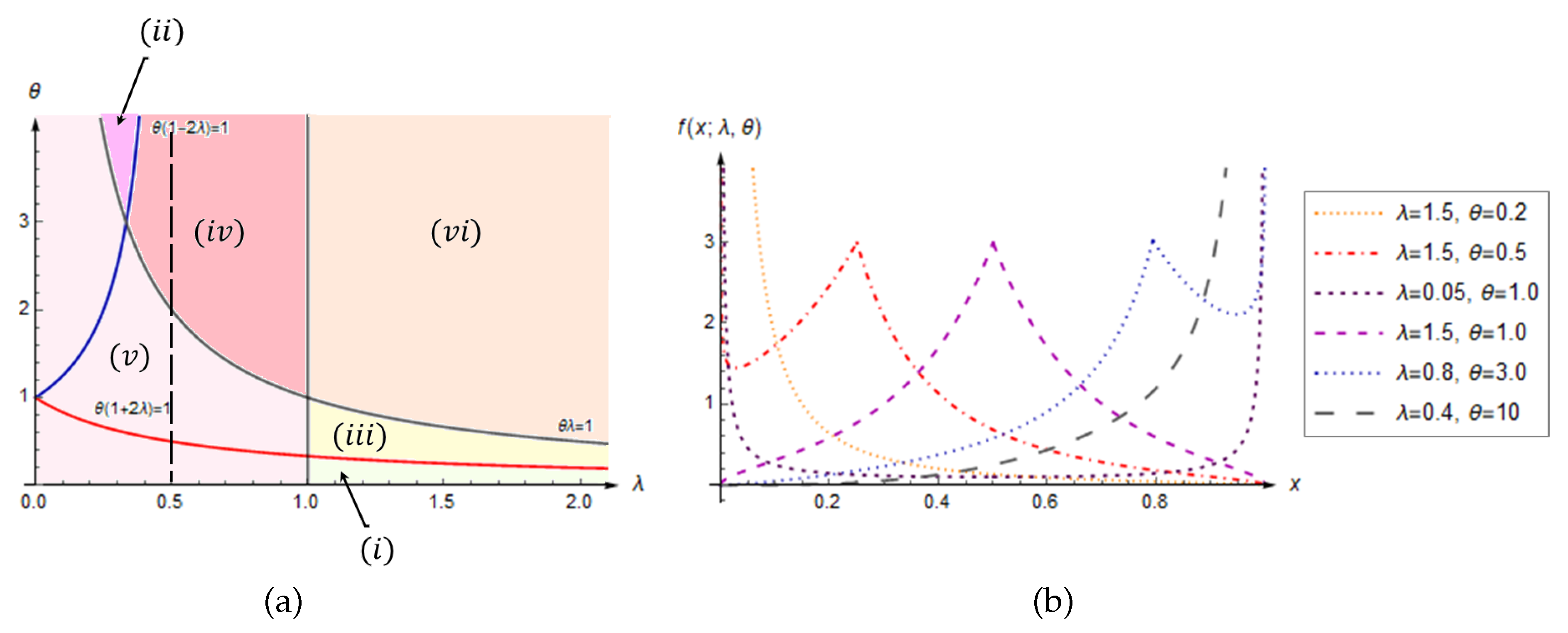
Figure 2.
3D Plots of the mean (a) and variance (b) of the LLU distribution, in dependence on parameters .
Figure 2.
3D Plots of the mean (a) and variance (b) of the LLU distribution, in dependence on parameters .
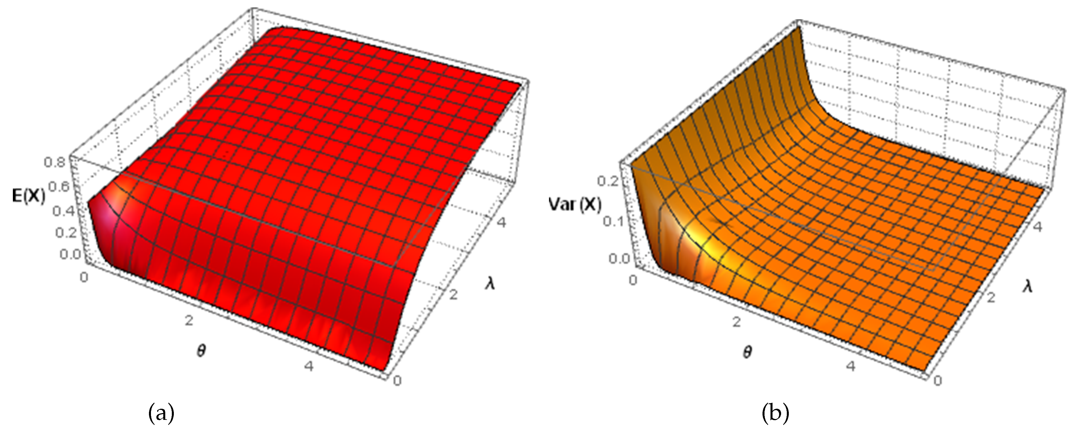
Figure 3.
Plots of the CDF (a) and HRF (b) of the LLU distribution, obtained with various parameters values .
Figure 3.
Plots of the CDF (a) and HRF (b) of the LLU distribution, obtained with various parameters values .
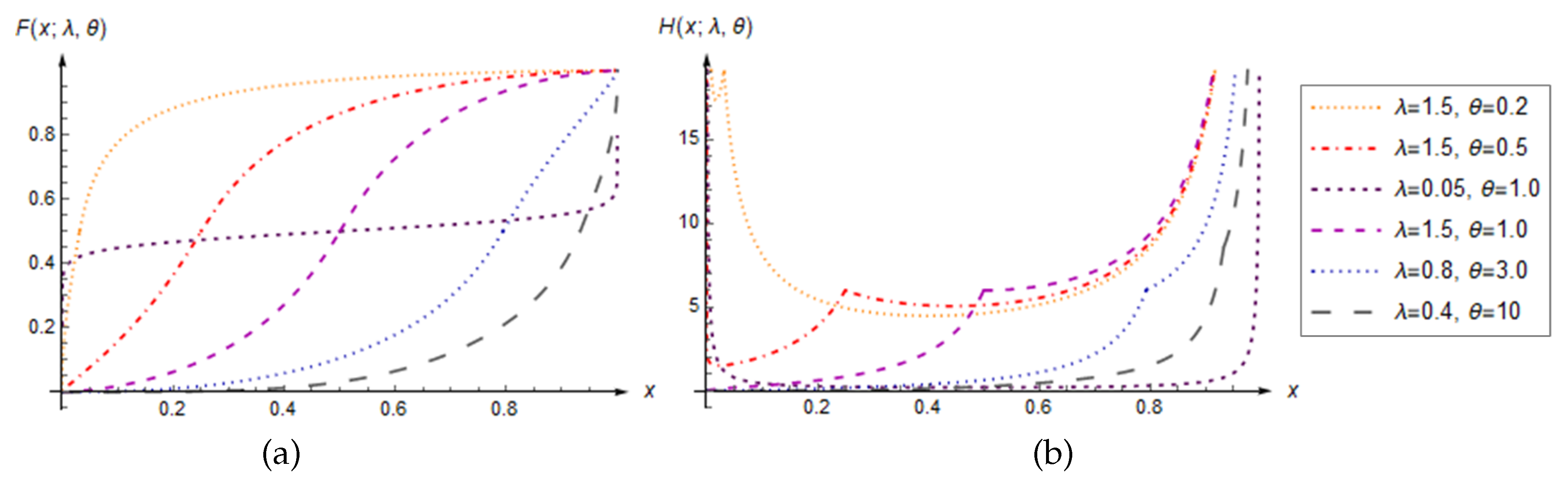
Figure 4.
3D graphs of the dependence of the coefficients of skewness and kurtosis with respect to the parameters .
Figure 4.
3D graphs of the dependence of the coefficients of skewness and kurtosis with respect to the parameters .
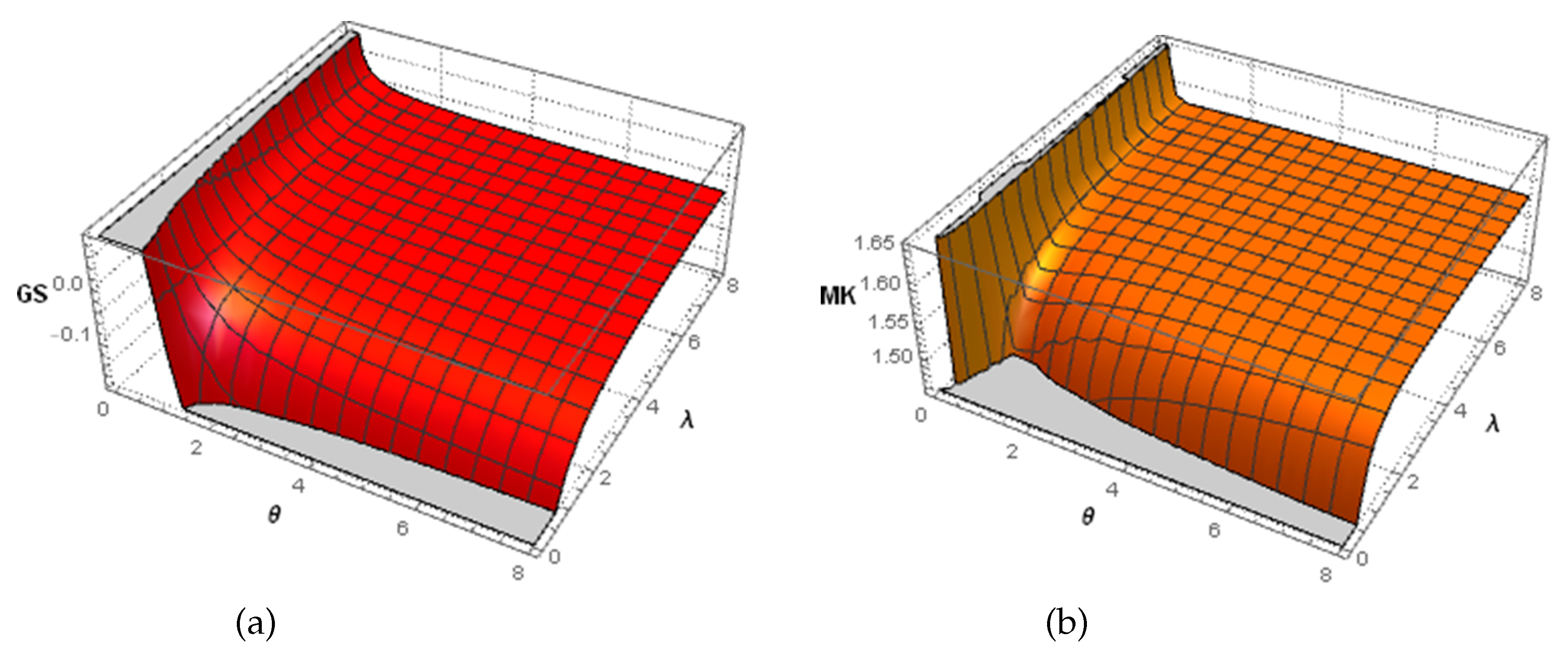
Figure 5.
Left plots: Realizations of the different samples taken from the LLU-distribution. Right plots: Empirical and fitted PDFs of the RV .
Figure 5.
Left plots: Realizations of the different samples taken from the LLU-distribution. Right plots: Empirical and fitted PDFs of the RV .
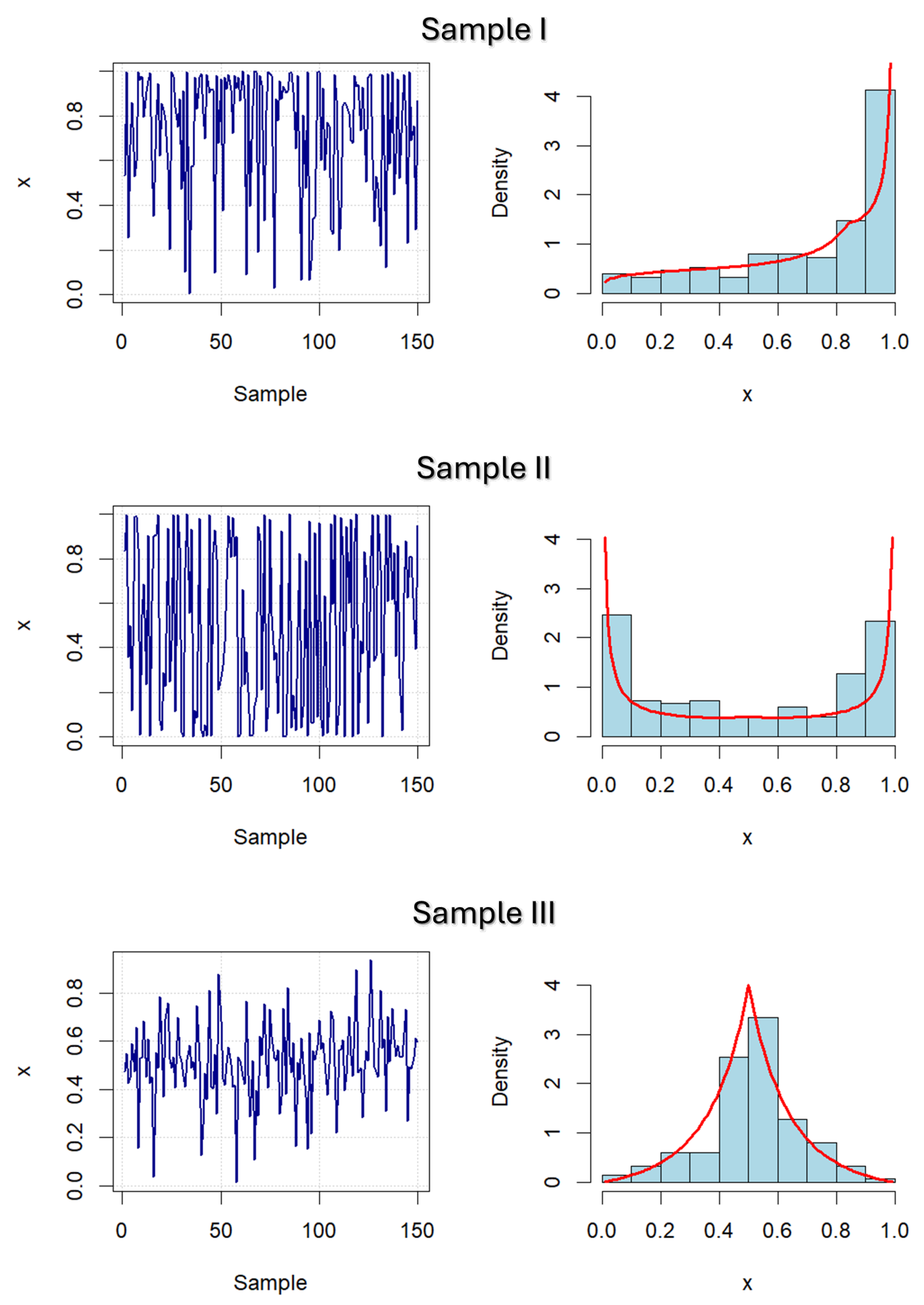
Figure 6.
Panels left: Observed values of the real-world data series. Panels right: Empirical and fitted PDFs, obtained with LLU, Beta and Kumaraswamy distributions.
Figure 6.
Panels left: Observed values of the real-world data series. Panels right: Empirical and fitted PDFs, obtained with LLU, Beta and Kumaraswamy distributions.
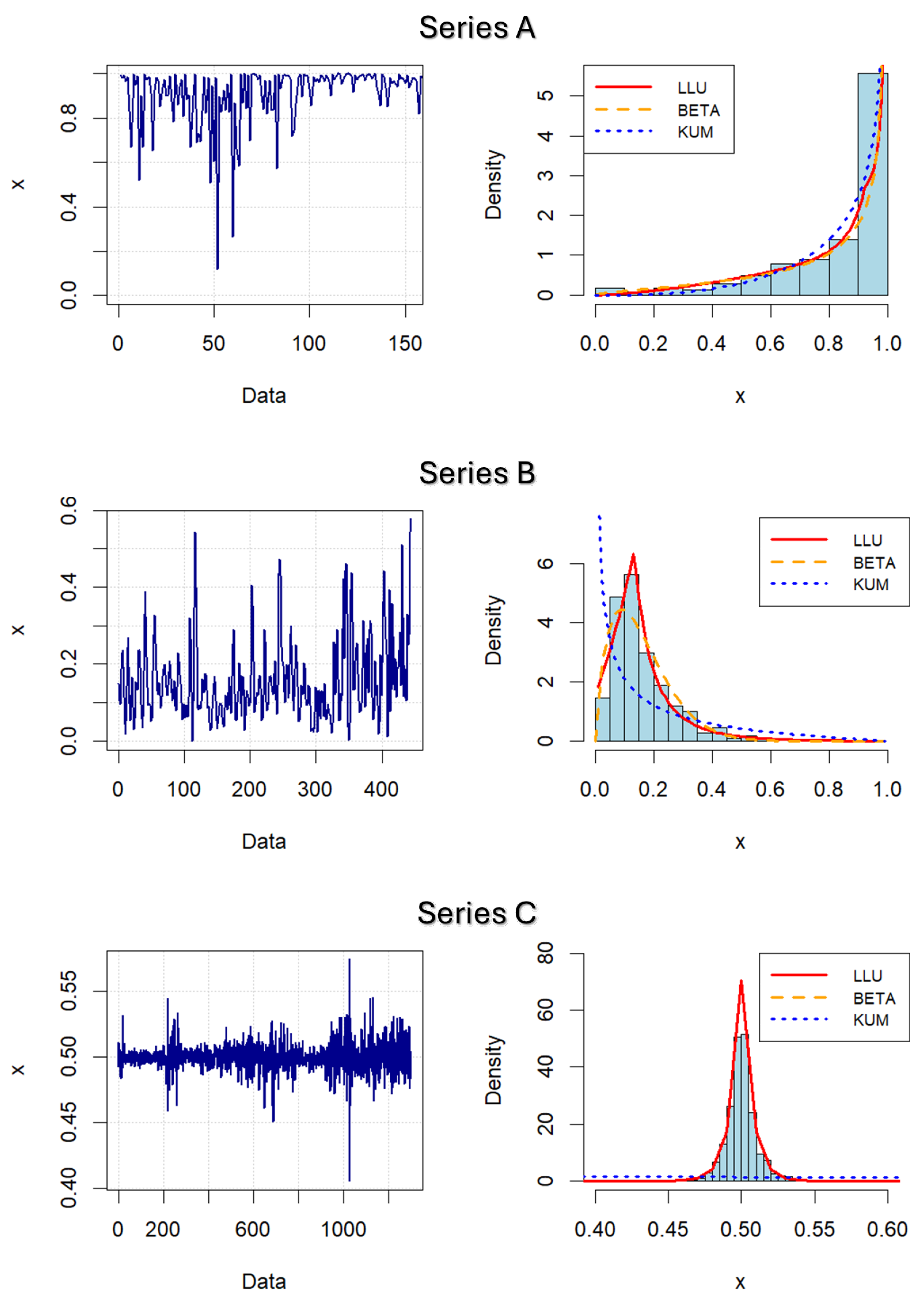

Table 1.
Summary statistics, estimation errors, and AN testing of parameters estimates of the LLU distribution. (Sample I with the parameters values: , ).
Table 1.
Summary statistics, estimation errors, and AN testing of parameters estimates of the LLU distribution. (Sample I with the parameters values: , ).
| Statistics | n = 150 | n = 500 | n = 1500 | |||||
|---|---|---|---|---|---|---|---|---|
| Min. | 1.770 | 0.1773 | 2.247 | 0.2190 | 2.676 | 0.2400 | ||
| Mean | 3.210 | 0.2850 | 3.378 | 0.2883 | 3.459 | 0.2928 | ||
| Max. | 5.907 | 0.4094 | 4.099 | 0.3660 | 3.650 | 0.3195 | ||
| SD | 0.0636 | 0.0448 | 0.0332 | 0.0260 | 0.0180 | 0.0150 | ||
| MSEE | 0.0790 | 0.0471 | 0.0722 | 0.0335 | 0.0712 | 0.0269 | ||
| FEE (%) | 8.286 | 15.715 | 3.486 | 11.029 | 1.171 | 8.959 | ||
| 0.8939 * | 1.6913 ** | 0.3090 | 0.6818 | 0.3796 | 0.1678 | |||
| (p-value) | (0.0221) | (2.38) | (0.5553) | (0.0739) | (0.4013) | (0.9359) | ||
* **
Table 2.
Summary statistics, estimation errors, and AN testing of parameters estimates of the LLU distribution. (Sample II with the parameters values: , ).
Table 2.
Summary statistics, estimation errors, and AN testing of parameters estimates of the LLU distribution. (Sample II with the parameters values: , ).
| Statistics | n = 150 | n = 500 | n = 1500 | |||||
|---|---|---|---|---|---|---|---|---|
| Min. | 0.5990 | 0.2161 | 0.7375 | 0.2369 | 0.8494 | 0.2602 | ||
| Mean | 1.0254 | 0.3054 | 1.0170 | 0.2987 | 1.0018 | 0.2968 | ||
| Max. | 1.8447 | 0.5394 | 1.4075 | 0.3824 | 1.2316 | 0.3477 | ||
| SD | 0.1907 | 0.0508 | 0.1224 | 0.0252 | 0.0698 | 0.0156 | ||
| MSEE | 0.0254 | 0.1169 | 0.0170 | 0.1019 | 0.0020 | 0.0981 | ||
| FEE (%) | 2.1346 | 34.453 | 0.5739 | 24.476 | 0.2030 | 21.908 | ||
| 1.1064 ** | 1.481 ** | 0.6684 | 0.8172 * | 0.5166 | 0.6030 | |||
| (p-value) | (6.58) | (7.83) | (0.0798) | (0.0341) | (0.1879) | (0.1159) | ||
* **
Table 3.
Summary statistics, estimation errors, and AN testing of parameters estimates of the LLU distribution. (Sample III with the parameters values: , ).
Table 3.
Summary statistics, estimation errors, and AN testing of parameters estimates of the LLU distribution. (Sample III with the parameters values: , ).
| Statistics | n = 150 | n = 500 | n = 1500 | |||||
|---|---|---|---|---|---|---|---|---|
| Min. | 0.9036 | 1.4760 | 0.9529 | 1.657 | 0.9698 | 1.860 | ||
| Mean | 1.0048 | 2.0360 | 1.0009 | 2.024 | 1.0003 | 2.016 | ||
| Max. | 2.6290 | 1.1179 | 1.0606 | 2.483 | 1.0262 | 2.243 | ||
| SD | 0.0305 | 0.2603 | 0.0166 | 0.1451 | 9.20 | 0.0767 | ||
| MSEE | 4.78 | 0.2621 | 8.88 | 0.1466 | 2.71 | 0.0782 | ||
| FEE (%) | 0.4783 | 13.106 | 0.0888 | 7.3314 | 0.0271 | 3.9117 | ||
| 0.4960 | 0.8509 * | 0.4029 | 0.2194 | 0.2951 | 0.3024 | |||
| (p-value) | (0.2113) | (0.0282) | (0.3539) | (0.8346) | (0.5930) | (0.5726) | ||
* **
Table 4.
Estimated parameters of the LLU, Beta and Kumaraswamy distribution, along with the corresponding estimation errors and fit statistics.
Table 4.
Estimated parameters of the LLU, Beta and Kumaraswamy distribution, along with the corresponding estimation errors and fit statistics.
| Paramet./ | Series A | Series B | Series C | ||||||||
|---|---|---|---|---|---|---|---|---|---|---|---|
| Statistics | LLU | BETA | KUM | LLU | BETA | KUM | LLU | BETA | KUM | ||
| 0.2972 | 1.6572 | 3.7527 | 2.5106 | 1.9375 | 0.4843 | 35.459 | 1133.27 | 1.4423 | |||
| 8.4338 | 0.3394 | 0.5241 | 0.3436 | 10.299 | 1.9341 | 0.9999 | 1133.21 | 2.1782 | |||
| MSEE | 0.0091 | 0.0139 | 0.0249 | 2.50 | 3.94 | 0.0205 | 1.31 | 2.28 | 0.0794 | ||
| AIC | -812.13 | -398.61 | -291.23 | -2671.99 | -891.80 | -687.07 | -17785.9 | -8173.7 | -325.18 | ||
| 0.0892 | 0.0797 | 0.1251 * | 0.0541 | 0.0676 | 0.3514 ** | 0.0215 | 0.0760 * | 0.5722 ** | |||
| (p-value) | (0.2534) | (0.3818) | (0.0347) | (0.5354) | (0.2629) | (0.00) | (0.9241) | (0.0108) | (0.00) | ||
* **
Disclaimer/Publisher’s Note: The statements, opinions and data contained in all publications are solely those of the individual author(s) and contributor(s) and not of MDPI and/or the editor(s). MDPI and/or the editor(s) disclaim responsibility for any injury to people or property resulting from any ideas, methods, instructions or products referred to in the content. |
© 2024 by the authors. Licensee MDPI, Basel, Switzerland. This article is an open access article distributed under the terms and conditions of the Creative Commons Attribution (CC BY) license (http://creativecommons.org/licenses/by/4.0/).
Copyright: This open access article is published under a Creative Commons CC BY 4.0 license, which permit the free download, distribution, and reuse, provided that the author and preprint are cited in any reuse.


