
Submitted:
23 September 2025
Posted:
23 September 2025
You are already at the latest version
Abstract
Statistical theory frequently involves adding a parameter to standard distributions. This work introduces a novel distribution called the Exponent Beta Exponential distribution. Several aspects of the proposed distribution are determined, the moment generating function (mgf), mode, quantiles and order statistics etc. The parameters were estimated the maximum likelihood estimation (MLE) technique. The proposed distribution was evaluated on two datasets. The proposed distribution outperforms over the various ver-sions of Exponential distributions based on model selection criteria’s.
Keywords:
MLE
; Beta Distribution
; Simulation
; Moments
; Distribution Function
MSC: 60E05; 60E10
1. Introduction
In recent decades, the development of statistical theory has increasingly focused on extending standard probability distributions. A common practice in this area involves the use of distribution generators, which introduce additional parameters to existing baseline distributions or combine multiple distributions, thereby enhancing flexibility and applicability [1]. Such modifications are primarily aimed at achieving better fits for complex datasets and facilitating the analysis of intricate data structures by refining classical models.
Pioneering contributions in this direction include the work of Mudholkar and Srivastava [2] and Marshall and Olkin [3], who introduced methods for incorporating new parameters into existing distributions. Eugene [4] advanced this line of research by proposing the beta-generated model, which was subsequently extended by Jones [5], who replaced the beta distribution with the Kumaraswamy distribution to construct a novel family of distributions. Further developments include the introduction of generalized continuous distributions by Alzaatreh et al. [6] and a comprehensive review of univariate distribution construction by Lee et al. [7]. More recently, Mahdavi and Kundu [8] proposed the Exponentiated Beta Pareto Distribution, which provides an additional mechanism for parameter insertion. The Exponentiated Beta Pareto Distribution is formally defined as:
Nassar et al. [9] employed the alpha power distribution as a generator to derive new density functions, which include the generalized exponential distribution [10], the Lindley distribution [11,13], and the exponential distribution [12]. The Pareto distribution (PD) has gained prominence as a model for data exhibiting heavy-tailed behavior [14] and has been applied across diverse fields, including the social sciences [15,16,17]. For instance, Philbrick [18] demonstrated the effectiveness of the PD in predicting insurance company losses and assessing hospital liability, while Levy and Levy [19] applied the exponential distribution to estimate societal wealth. Similarly, Castillo and Hadi [20] employed a generalized Pareto distribution to model flood control exceedances. The literature documents a wide variety of Pareto distributions and their generalizations, reflecting their versatility in statistical modeling. As noted by Johnson [21], the probability density function (pdf) of the exponential distribution is given by:
where denotes the scale parameter of the distribution. The corresponding cumulative distribution function (cdf) is expressed as:
The reversed J-shaped, decreasing hazard function of the Pareto distribution (PD) does not always provide an adequate fit to empirical data. In risk and reliability analysis, alternative approaches are often required to model loss, risk, or life-cycle behavior. For example, Gupta et al. [23] and Nadarajah [24] demonstrated that human mortality patterns can be more flexibly modeled using adaptive distributions [17]. Notable alternatives include the Weibull distribution [27,28], the Generalized distribution [22], the Exponentiated distribution, the Beta-Generalized distribution [26], the Exponentiated Weibull distribution [31], the Burr X-P distribution [17], and the Exponentiated Generalized distribution [14].
To enhance the flexibility of the basic PD, we introduce an additional parameter. The subsequent sections examine several theoretical and practical aspects of the proposed Exponentiated Beta Pareto (EBE) distribution. Specifically, stochastic ordering properties are established in Lemmas 1 and 2. Parameter estimation is then addressed through the maximum likelihood method, supported by simulation studies. Finally, the concluding section summarizes key findings and highlights directions for further research.
2. Exponent Beta Exponential (EBE) Distribution
Let X be a random variable that follows the Exponentiated Beta Pareto (EBE) distribution. Its pdf and cdf are defined, respectively, as:
Figure 1 belw presents the pdf and cdf of the EBE distribution for various values of the parameters. These graphical representations illustrate the flexibility of the EBE distribution in modeling diverse data patterns through variation in its parameter values.
The survival function S(x) and the hazard rate function h(x) corresponding to the (EBE) distribution are expressed as:
Figure 2 illustrates the hazard rate function of the EBE distribution for selected values of the shape parameters and . The plots highlight the sensitivity of the hazard rate to changes in these parameters, thereby demonstrating the flexibility of the EBE distribution in capturing diverse lifetime behaviors.
2.1. Quantile Function
For a random variable , the quantile function , can be derived by inverting its cumulative distribution function. Specifically,
where U follows conventional uniform distribution and yield:
For median, substituting into the quantile function (Equation (10)), which yield:
2.2. Mode
The mode of the distribution is determined as the solution to the first-order condition of the pdf, obtained by setting the derivative of the log-likelihood with respect to xxx equal to zero. Explicitly, it satisfies the following equation:
By differentiating Equation (6) with respect to x and equating the result to zero, the mode of the distribution is obtained as the solution of the following expression:
2.3. rth Raw Moment
By definition, the rth raw moment of a random variable X with pdf f(x) is expressed as:
2.4. Moment Generating Function
The moment generating function (mgf) of a random variable X is defined as:
Simplifying the above expression yields the following result:
Lemma 1:
Let X1~EBE (α1, β,) and X2~ EBE (α2, β,).
If α1 < α2 then
2.5. Order Statistics
The order statistic, denoted , of a random sample from a distribution with cdf and pdf , has the pdf given by:
Here
By substituting the corresponding expressions for and f from the EBE distribution into Equation (16), the probability density function of the order statistic is obtained as follows:
By setting in Equation (17), the density function of the smallest (first) order statistic is obtained as:
By setting in Equation (17), the density function of the largest order statistic is obtained as:
2.6. Stress-Strength Parameter (SSP)
If and are two independent random variables, where ~EBE() and ~EBE(), the SSP is given by:
Using series
Substituting the series expansion into Equation (19) yield:
2.7. Parameter Estimations
In this part, we use a complete sample to determine the maximum probability estimates of the unknown parameters , and . Assume that we have a basic random sample from EBE(α, β,) with the following values: , , .
Taking the likelihood of the sample gives:
By differentiating Equation (20) with respect to the parameter , we obtain:
By differentiating Equation (20) with respect to the parameter , we obtain:
By differentiating Equation (20) with respect to the parameter , we obtain:
By differentiating Equation (21) with respect to the parameter , we obtain:
By differentiating Equation (21) with respect to the parameter , we obtain:
By differentiating Equation (21) with respect to the parameter , we obtain:
By differentiating Equation (22) with respect to the parameter , we obtain:
By differentiating Equation (23) with respect to the parameter , we obtain:
3. Simulations Study
A Monte Carlo simulation study was conducted to examine the bias, mean square error (MSE), and average values of the maximum likelihood estimators (MLEs). Specifically, random samples were generated from the EBE distribution for sample sizes , and . The random variates were obtained using the following transformation formula:
where U denotes the standard uniform random variate.
The bias and MSE of the maximum likelihood estimators were computed using the following expressions:
In the above expressions, represents the true value of the parameter, while denotes its corresponding maximum likelihood estimate obtained from the simulated samples.
Table 1 presents the average bias and MSE values of the estimators. The results indicate that the estimates are consistent and remain close to the true parameter values across all scenarios. Furthermore, an increase in sample size leads to a reduction in both MSE and bias for all parameter combinations, demonstrating the efficiency of the estimators. Overall, the maximum likelihood estimation procedure provides accurate and reliable estimates of the parameters of the EBE distribution.
4. Real Data Application
To assess the practical performance of the proposed EBE distribution, two real data sets are analyzed. The objective of this section is to evaluate the goodness-of-fit of the EBE distribution and to compare its performance with other related models, including the exponential [35], Beta Generalized Exponential (BGE) [22], and Alpha Power Exponentiated Inverse Exponential (APEIE) [14,29,36] distributions. Parameter estimates are obtained using the method of maximum likelihood, and model comparisons are conducted based on standard statistical criteria such as the log-likelihood, Akaike Information Criterion (AIC), Bayesian Information Criterion (BIC), and Kolmogorov–Smirnov (K–S) test. These measures provide a comprehensive assessment of the adequacy of the proposed model in fitting real-world data. For clarity, the corresponding probability density functions (pdfs) of these distributions are provided below:
- Exponential distribution (ED)
- BGE distribution
- APEIE distribution
To demonstrate the practical applicability and effectiveness of the proposed model, two real data sets are analyzed.
Data Set 1: Application on Cancer data
The first data set consists of survival times (in months) of 121 breast cancer patients treated at a large hospital during the period 1929–1938, as originally reported by [38]. These observations have been widely used in the statistical literature to evaluate lifetime distributions and serve as a benchmark for comparing model performance. The data are presented as follows:
0.3, 0.3, 4.0, 5.0, 5.6, 6.2, 6.3, 6.6, 6.8, 7.4, 7.5, 8.4, 8.4, 10.3, 11.0, 11.8, 12.2, 12.3, 13.5, 14.4, 14.4, 14.8, 15.5, 15.7, 16.2, 16.3, 16.5, 16.8, 17.2, 17.3, 17.5, 17.9, 19.8, 20.4, 20.9, 21.0, 21.0, 21.1, 23.0, 23.4, 23.6, 24.0, 24.0, 27.9, 28.2, 29.1, 30.0, 31.0, 31.0, 32.0, 35.0, 35.0, 37.0, 37.0, 37.0, 38.0, 38.0, 38.0, 39.0, 39.0, 40.0, 40.0, 40.0, 41.0, 41.0, 41.0, 42.0, 43.0, 43.0, 43.0, 44.0, 45.0, 45.0, 46.0, 46.0, 47.0, 48.0, 49.0, 51.0, 51.0, 51.0, 52.0, 54.0, 55.0, 56.0, 57.0, 58.0, 59.0, 60.0, 60.0, 60.0, 61.0, 62.0, 65.0, 65.0, 67.0, 67.0, 68.0, 69.0, 78.0, 80.0, 83.0, 88.0, 89.0, 90.0, 93.0, 96.0, 103.0, 105.0, 109.0, 109.0, 111.0, 115.0, 117.0, 125.0, 126.0, 127.0, 129.0, 129.0, 139.0, 154.0
Table 2 reports the model diagnostics for Data Set 1 based on the fitted EBE distribution and its competing models. The results show that the EBE achieves the lowest AIC, BIC, CAIC, and HQIC values among all candidate models, indicating superior overall fit. Moreover, the K–S test yields a p-value of 0.3501 for the EBE, which is considerably higher than those obtained for the alternative models, thereby supporting its adequacy in describing the data. In contrast, the BGE and APEIE exhibit much larger information criteria values and extremely small p-values, suggesting poor fit. While the exponential distribution (ED) performs moderately well, its fit is still inferior to that of the EBE, as reflected by both higher information criteria and a lower p-value (0.05971). Taken together, these diagnostics confirm that the proposed EBED provides the best fit to the breast cancer survival data compared to the considered competing models. Hence, the EBED can be regarded as a more flexible and reliable alternative to the exponential and related lifetime distributions for modeling survival data.
A graphical assessment of the fitted EBE distribution was also carried out using histograms of the empirical data overlaid with the fitted density curves, Q–Q plots, and empirical versus theoretical cumulative distribution functions (CDFs). Figure 3 shows that the EBE closely follows the observed frequency distribution, while QQ-plot values deviate from the fitted line, this is typical of heavy-tailed distributions [37]. In addition, the empirical and fitted CDFs display a close match across the entire range of the data. These graphical diagnostics further support the numerical results, confirming that the EBE distribution provides an excellent fit to the data compared to competing models.
Figure 4 presents graphical diagnostics for Data Set 1. The left panel compares the histogram of the empirical data with the fitted theoretical densities of the competing models (EBE, ED, BGE, and APEIE). The EBE curve (solid red) aligns closely with the shape of the observed data across the entire range, whereas the alternative models either underestimate the peak or fail to capture the tail behavior effectively. The right panel shows the empirical cumulative distribution function (CDF) plotted against the fitted CDFs of the competing models. Once again, the EBE provides the best agreement, with its theoretical cdf (solid red) almost overlapping the empirical cdf throughout. In contrast, the BGE and APEIE curves deviate substantially from the empirical distribution, particularly in the lower and middle quantiles, while the ED shows moderate but inferior fit compared to EBE. Overall, both the pdf and cdf plots confirm that the EBE offers a superior fit to the breast cancer survival data relative to the competing models.
Data Set 2: Application on earthquakes in the last century
The second dataset consists of the time intervals of the successive earthquakes in the last century in the North Anatolia fault zone originally reported by [17,34].
3.70,2.74,2.73,2.50,3.60,3.11,3.27, 2.87, 1.47, 3.11, 4.42, 2.41, 3.19, 3.22, 1.69, 3.28, 3.09, 1.87, 3.15,4.90,3.75,2.43,2.95,2.97,3.39,2.96,2.53,2.67,2.93,3.22,3.39,2.81,4.20,3.33,2.55,3.31,3.31, 2.85,2.56,3.56,3.15,2.35,2.55,2.59,2.38,2.81,2.77,2.17,2.83,1.92,1.41,3.68,2.97,1.36,0.98,2.76,4.91,3.68,1.84,1.59,3.19,1.57,0.81,5.56,1.73,1.59,2.00,1.22,1.12,1.71,2.17,1.17,5.08,2.48,1.18,3.51,2.17,1.69,1.25,4.38,1.84,0.39,3.68,2.48,0.85,1.61,2.79,4.70,2.03,1.80,1.57,1.08,2.03,1.61,2.12, 1.89,2.88,2.82,2.05,3.65
The goodness-of-fit results provided in Table 3 show that among the considered models, the EBED distribution provides the best fit to the dataset. It achieves the lowest AIC, CAIC, BIC, and HQIC values compared to the other competing models. Moreover, its p-value (0.4091) is well above the conventional significance level (0.05), indicating that the EBED cannot be rejected as a plausible model. In contrast, the ED and APEIED models yield very low p-values, suggesting a poor fit, while the BGED performs moderately well but still inferior to EBED based on both information criteria and p-value.
Figure 5 show that the proposed distribution fits the data well. The histogram of the data is closely matched by the fitted theoretical density curve (red line), showing a good alignment between observed and expected frequencies. The points lie approximately along the 45° reference line, indicating that the quantiles of the fitted distribution are in strong agreement with the sample quantiles. The empirical cumulative distribution function (black circles) aligns well with the theoretical CDF (red line), further confirming the adequacy of the model. The observed probabilities track the theoretical probabilities closely along the diagonal, suggesting no major deviations in fit.
5. Discussion
The Exponentiated Beta Exponential (EBE) distribution was introduced and studied through its fundamental properties, including order statistics, stress–strength reliability, mode, and stochastic ordering. Parameter estimation was carried out using the Maximum Likelihood Estimation (MLE) method. The performance of the proposed EBE distribution was evaluated against other competing probability models using two real-life datasets.
Model comparison criteria (AIC, BIC, CAIC, and HQIC) consistently indicated that the EBE distribution provided a superior fit. Furthermore, goodness-of-fit diagnostics; such as histograms with fitted densities, Q–Q plots, CDF plots, and P–P plots; demonstrated that the EBE model closely matched the empirical data, confirming its suitability. Overall, the findings highlight that the EBE distribution is a flexible and reliable model that outperformed other well-known distributions in capturing the characteristics of the studied datasets.
6. Conclusions
The distribution, known as the EBE, is introduced using Exponent Beta Exponential Distribution. Topics covered include function, order statistics, stress strength, mode, stochastic ordering. The maximum likelihood estimation approach was utilized to obtain parameter estimates for unknown parameters. The proposed distribution outperformed other Exponential distributions on two real datasets.
Author Contributions
Sofia contributed to the conceptualization, methodology, data curation, and writing of the original draft. Muhammad Asif was responsible for formal analysis, investigation, validation, and writing—review and editing. Muhammad Atif provided supervision, project administration, and writing—review and editing. Muhammad Farooq contributed resources, data curation, and validation. S. Al-Moisheer was involved in formal analysis and writing—review and editing. Muhammad Ali contributed through supervision and project administration.
Funding
This work was supported and funded by the Deanship of Scientific Research at Imam Mohammad Ibn Saud Islamic University (IMSIU) (grant number IMSIU-DDRSP2504).
Data Availability Statement
Data is contained within the article
Conflicts of Interest
The authors declare no conflicts of interest
Abbreviations
The following abbreviations are used in this manuscript:
| EBE | Exponentiated Beta Exponential Distribution |
| ED | Exponential Distribution |
| BGED | Beta Generalized Exponential Distribution |
| APEIED | Alpha Power Exponentiated Inverse Exponential Distribution |
References
- Dey S, Sharma VK, Mesfioui M. A new extension of Weibull distribution with application to lifetime data.Annals of Data Science. 2017; 4(1):31–61. [CrossRef]
- Mudholkar G S, Srivastava DK. Exponentiated Weibull family for analyzing bathtub failure-rate data.IEEE transactions on reliability. 1993; 42(2):299–302. [CrossRef]
- Marshall AW, Olkin I. A new method for adding a parameter to a family of distributions with application to the exponential and Weibull families. Biometrika. 1997; 84(3):641–52. [CrossRef]
- Eugene N, Lee C, Famoye F. Beta-normal distribution and its applications. Communications in Statistics-Theory and methods. 2002; 31(4):497–512. [CrossRef]
- Jones M. C. Kumaraswamy’s distribution: A beta-type distribution with some tractability advantages.Statistical Methodology. 2009; 6(1):70–81. [CrossRef]
- Alzaatreh A, Lee C, Famoye F. A new method for generating families of continuous distributions.Metron. 2013; 71(1):63–79. [CrossRef]
- Lee C, Famoye F, Alzaatreh AY. Methods for generating families of univariate continuous distributionsin the recent decades. Wiley Interdisciplinary Reviews: Computational Statistics. 2013; 5(3):219–38. [CrossRef]
- Mahdavi A, Kundu D. A new method for generating distributions with an application to exponential distribution.Communications in Statistics-Theory and Methods. 2017; 46(13):6543–57. [CrossRef]
- Nassar M, Alzaatreh A, Mead M, Abo-Kasem O. Alpha power Weibull distribution: Properties and applications.Communications in Statistics-Theory and Methods. 2017 18; 46(20):10236–52. [CrossRef]
- Dey S, Alzaatreh A, Zhang C, Kumar D. A new extension of generalized exponential distribution with application to Ozone data. Ozone: Science & Engineering. 2017; 39(4):273–85. [CrossRef]
- Dey S, Ghosh I, Kumar D. Alpha-Power Transformed Lindley Distribution: Properties and Associated Inference with Application to Earthquake Data. Annals of Data Science. 2018:1–28. [CrossRef]
- Hassan AS, Mohamd RE, Elgarhy M, Fayomi A. Alpha power transformed extended exponential distribution: properties and applications. Journal of Nonlinear Sciences and Applications. 2018; 12(4), 62–67. [CrossRef]
- Dey S, Nassar M, Kumar D. Alpha power transformed inverse Lindley distribution: A distribution with an upside-down bathtub-shaped hazard function. Journal of Computational and Applied Mathematics.2019; 348:130–45. [CrossRef]
- Lee S, Kim J H. Exponentiated generalized Pareto distribution: Properties and applications towards extreme value theory. Communications in Statistics-Theory and Methods. 2018; 1–25. [CrossRef]
- Brazauskas V, Serfling R. Favorable estimators for fitting Pareto models: A study using goodness-of-fit measures with actual data. ASTIN Bulletin: The Journal of the IAA. 2003; 33(2):365–81. [CrossRef]
- Farshchian M, Posner F L. The Pareto distribution for low grazing angle and high resolution X-band sea clutter. Naval Research Lab Washington DC; 2010. [CrossRef]
- Korkmaz M, Altun E, Yousof H, Afify A, Nadarajah S. The Burr X Pareto Distribution: Properties, Applications and VaR Estimation. Journal of Risk and Financial Management. 2018; 11(1):1. [CrossRef]
- Philbrick S W. A practical guide to the single parameter Pareto distribution. PCAS LXXII. 1985; 44–85.
- Levy M, Levy H. Investment talent and the Pareto wealth distribution: Theoretical and experimentalanalysis. Review of Economics and Statistics. 2003; 85(3):709–25. [CrossRef]
- Castillo E, Hadi AS. Fitting the generalized Pareto distribution to data. Journal of the American StatisticalAssociation. 1997; 92(440):1609–20. [CrossRef]
- Johnson N. L., and Kotz S., Balakrishnan N. Continuous Univariate Distributions-I. New York: JohnWiley; 1994.
- Pickands J III. Statistical inference using extreme order statistics. The Annals of Statistics. 1975;3(1):119–31.
- Gupta RC, Gupta PL, Gupta RD. Modeling failure time data by Lehman alternatives. Communicationsin Statistics-Theory and methods. 1998; 27(4):887–904. [CrossRef]
- Nadarajah S. Exponentiated Pareto distributions. Statistics. 2005; 39(3):255–60. [CrossRef]
- Akinsete A, Famoye F, Lee C. The beta-Pareto distribution. Statistics. 2008; 42(6):547–63. [CrossRef]
- Mahmoudi E. The beta generalized Pareto distribution with application to lifetime data. Mathematicsand computers in Simulation. 2011; 81(11):2414–30. [CrossRef]
- Alzaatreh A, Famoye F, Lee C. Weibull-Pareto distribution and its applications. Communications in Statistics-Theory and Methods. 2013; 42(9):1673–91. [CrossRef]
- Tahir M H, Cordeiro GM, Alzaatreh A, Mansoor M, Zubair M. A new Weibull–Pareto distribution: propertiesand applications. Communications in Statistics-Simulation and Computation. 2016; 45(10):3548–67. [CrossRef]
- Pereira MB, Silva RB, Zea LM, Cordeiro GM. The kumaraswamy Pareto distribution. arXiv preprintarXiv:1204.1389. 2012. [CrossRef]
- Nadarajah S, Eljabri S. The kumaraswamy gp distribution. Journal of Data Science. 2013; 11(4):739–66.
- Afify AZ, Yousof HM, Hamedani GG, Aryal G. The exponentiated Weibull-Pareto distribution with application.J. Stat. Theory Appl. 2016; 15:328–46. [CrossRef]
- Shaked M, Shanthikumar Jeyaveerasingam G. Stochastic Orders. Series: Springer Series in Statistics.New York: Springer; 2007.
- Hogg R. and Klugman S.A. Loss Distributions. New York: Wiley; 1984.
- Mead ME, Afify AZ, Hamedani GG, Ghosh I. The beta exponential Fre’chet distribution with applications.Austrian Journal of Statistics. 2017; 46(1):41–63.
- Johnson N. L., and Kotz S. Continuous Univariate Distributions-2. Boston: Houghton Mifflin; 1970.
- Guo L, Gui W. Bayesian and Classical Estimation of the Inverse Pareto Distribution and Its Application to Strength-Stress Models. American Journal of Mathematical and Management Sciences. 2018; 37(1):80–92. [CrossRef]
- Brodin E, Rootze’n H. Univariate and bivariate GPD methods for predicting extreme wind storm losses.Insurance: Mathematics and Economics. 2009; 44(3):345–56. [CrossRef]
- Ramos, M.W.A., Cordeiro, G.M., Marinho, P.R.D., Dias, C.R.B. and Hamedani, G.G.(2013). The Zografos-Balakrishnan log-logistic distribution: Properties andapplications. Journal of Statistical Theory and Applications, 12, 225-244. [CrossRef]
Figure 1.
PDF and CDF of Exponent Beta Exponential Distribution.
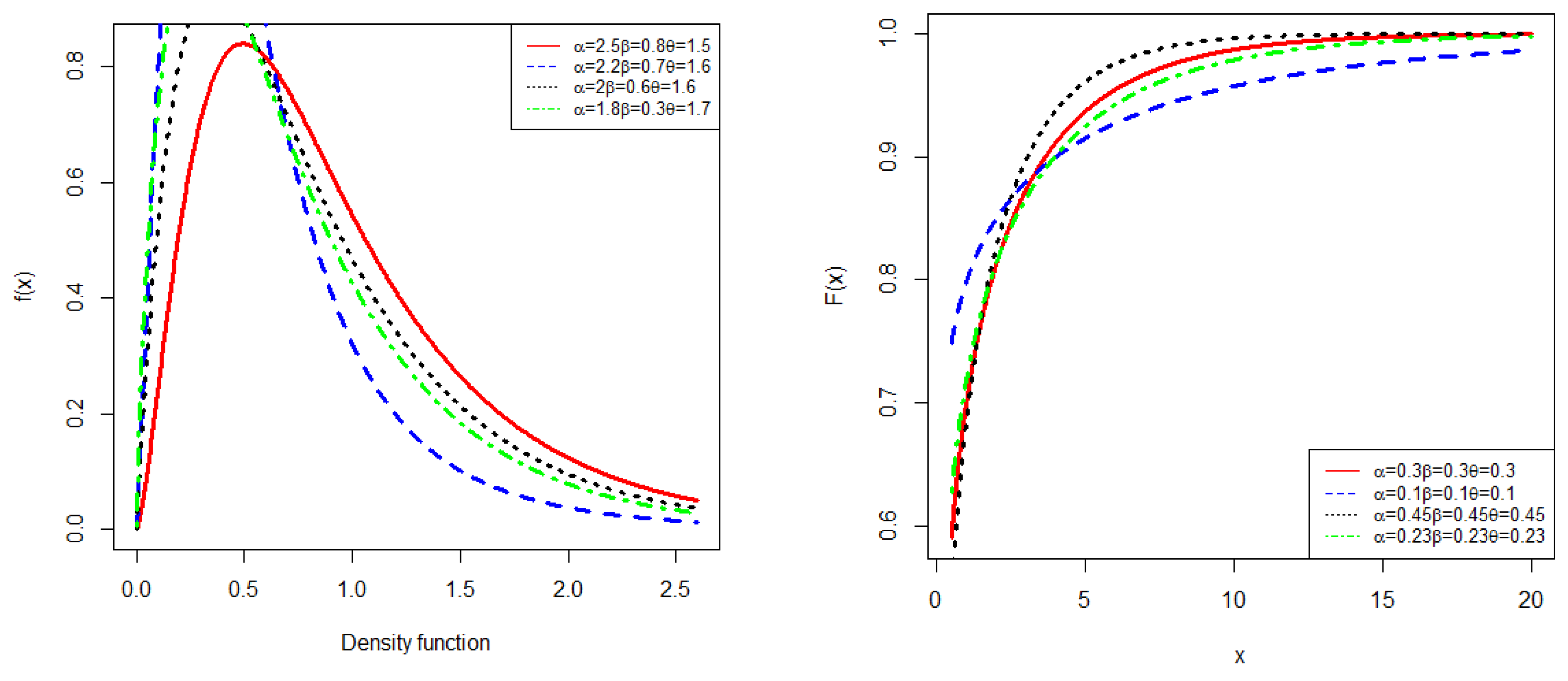
Figure 2.
Hazard rate of Exponent Beta Exponential Distribution.
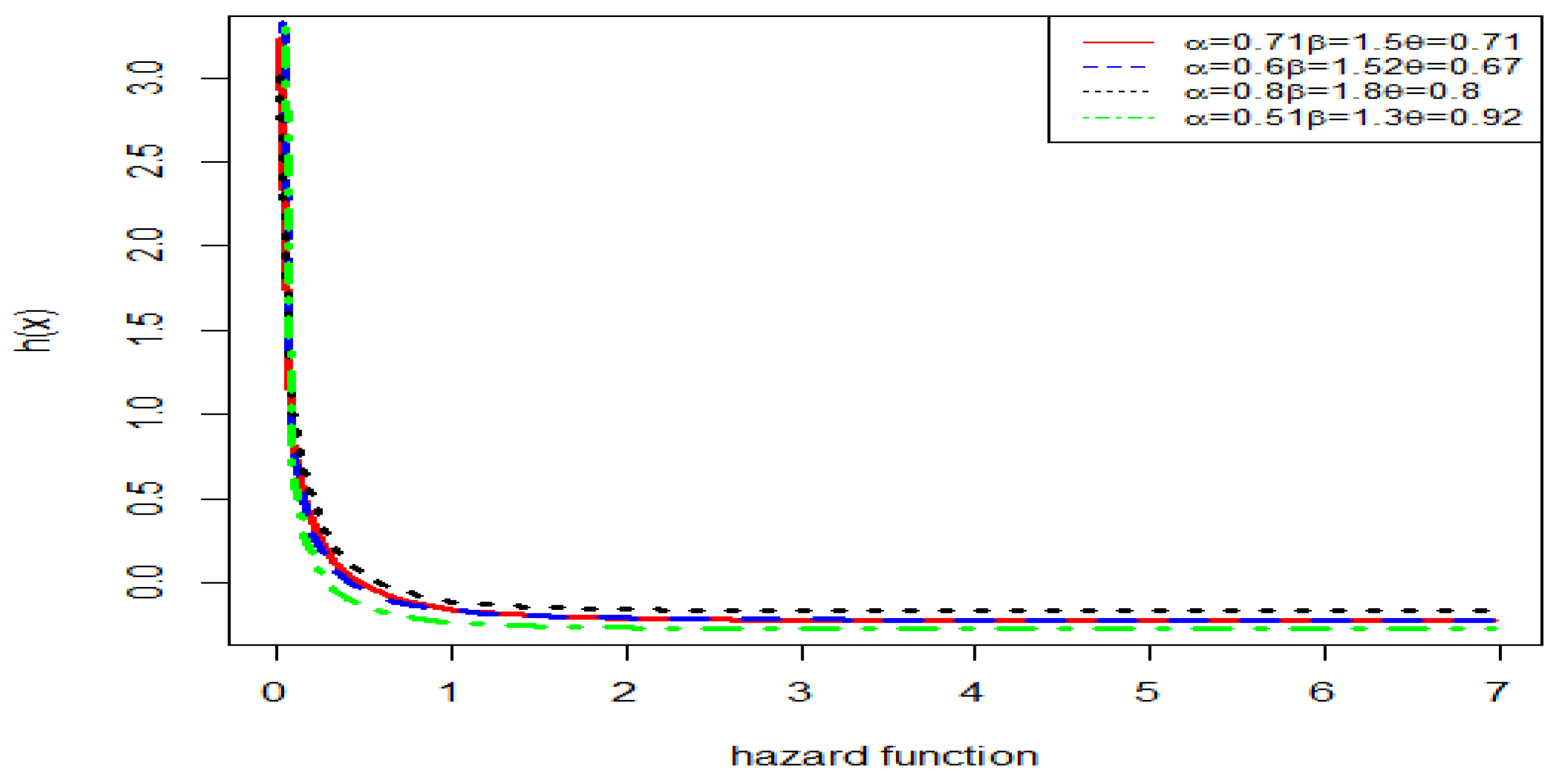
Figure 3.
QQ-plot and PP-plot for data set 1.
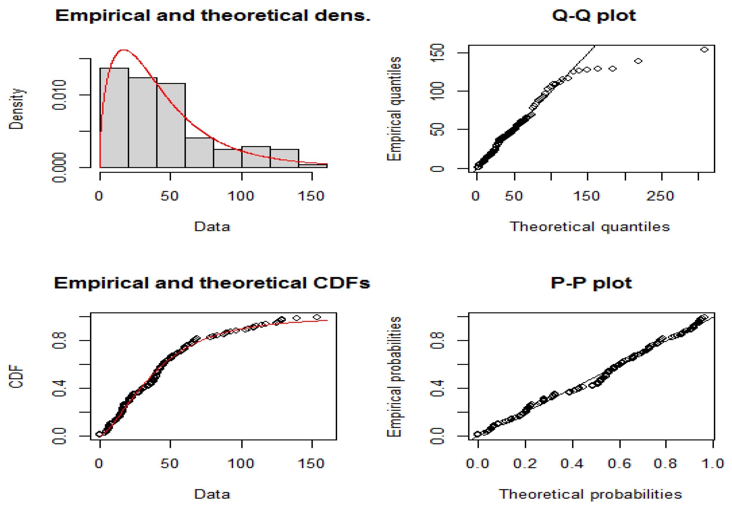
Figure 4.
Comparison of EBE Distribution with other competitive models for data set 1.
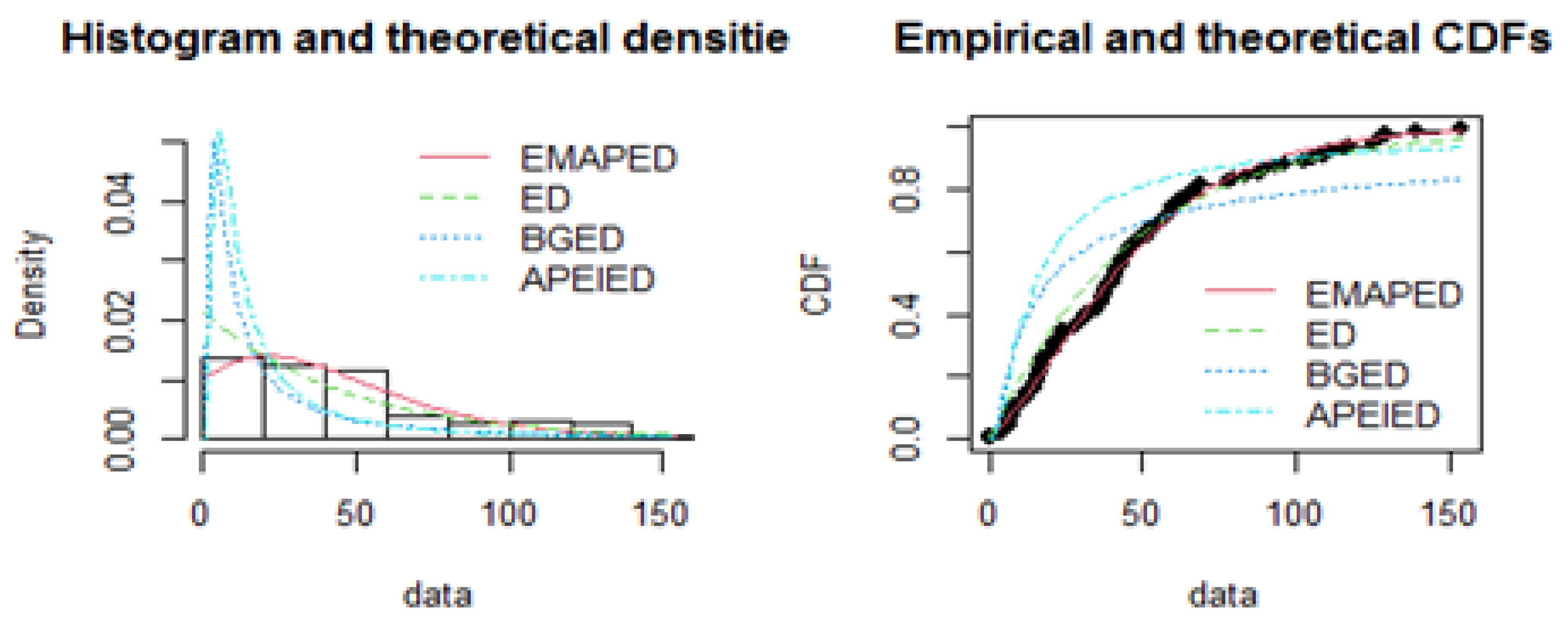
Figure 5.
QQ-plot and PP-plot for data set 2.
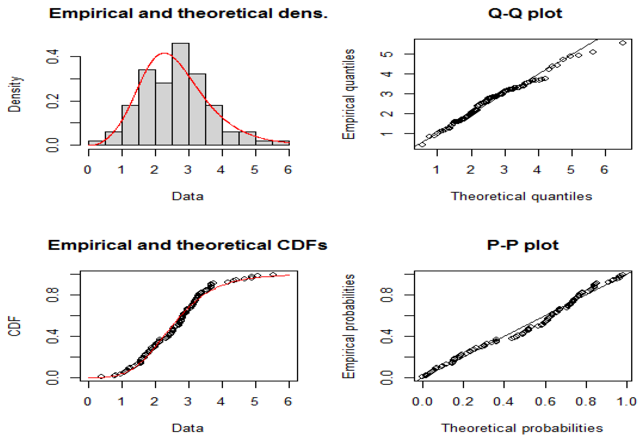

Table 1.
Bias and MSE of EBE Distribution.
| Parameters | N | MSE0 | MSE1 | MSE2 | BIAS0 | BIAS1 | BIAS2 |
|---|---|---|---|---|---|---|---|
|
|
60 | 0.25942 | 9.90072 | 7.8970 | 0.03388 | -0.83549 | 1.49541 |
| 150 | 0.08497 | 4.96927 | 3.9120 | 0.03255 | -0.41015 | 0.75848 | |
| 230 | 0.05041 | 3.70697 | 2.9987 | 0.00723 | -0.08396 | 0.50724 | |
|
|
40 | 0.22716 | 15.6961 | 7.0710 | 0.11502 | -0.66054 | 1.48416 |
| 130 | 0.08807 | 8.56222 | 4.6855 | 0.02997 | -0.05309 | 0.81565 | |
| 210 | 0.03797 | 3.81034 | 2.4992 | -0.02088 | -0.04777 | 0.44718 | |
|
|
120 | 0.07721 | 5.25017 | 4.3567 | 0.10494 | -0.79556 | 1.18455 |
| 220 | 0.03589 | 2.01053 | 2.0358 | 0.03613 | -0.07332 | 0.38506 | |
| 380 | 0.03043 | 2.32888 | 2.0092 | -0.0011 | -0.02987 | 0.37981 |
Table 2.
Model Diagnostics for Data Set 1.
| Distribution | MLE | AIC | CAIC | BIC | HQIC | P-value | ||
| EBE | 1.454518 | 0.205884 | 0.025538 | 1166.945 | 1167.15 | 1175.333 | 1170.352 | 0.3501 |
| ED | 0.021593 | 1172.256 | 1172.28 | 1175.051 | 1173.391 | 0.05971 | ||
| BGED | 0.560161 | 6.3926366 | 1332.248 | 1332.35 | 1337.84 | 1334.519 | 1.141e-08 | |
| APEIED | 3.587380 | 24.433696 | 1.533854 | 1264.878 | 1265.083 | 1273.266 | 1268.285 | 2.2e-16 |
Table 3.
Model Diagnostics for Data Set 2.
| Distribution | MLE | AIC | CAIC | BIC | HQIC | P-value | ||
| EBE | 4.724535 | -3.409094 | 1.244129 | 291.6781 | 291.9281 | 299.4936 | 294.8412 | 0.4091 |
| ED | 0.3814557 | 394.7417 | 394.7825 | 397.3469 | 395.7961 | 2.369e-09 | ||
| BGED | 9.060031 | 6.196268 | 306.4821 | 306.6058 | 311.6924 | 308.5908 | 0.06698 | |
| APEIED | 1.057584 | 2.023400 | 402.7912 | 402.9149 | 408.0015 | 404.8999 | 2.315e-11 | |
Disclaimer/Publisher’s Note: The statements, opinions and data contained in all publications are solely those of the individual author(s) and contributor(s) and not of MDPI and/or the editor(s). MDPI and/or the editor(s) disclaim responsibility for any injury to people or property resulting from any ideas, methods, instructions or products referred to in the content. |
© 2025 by the authors. Licensee MDPI, Basel, Switzerland. This article is an open access article distributed under the terms and conditions of the Creative Commons Attribution (CC BY) license (http://creativecommons.org/licenses/by/4.0/).
Copyright: This open access article is published under a Creative Commons CC BY 4.0 license, which permit the free download, distribution, and reuse, provided that the author and preprint are cited in any reuse.


