
Submitted:
17 April 2024
Posted:
18 April 2024
You are already at the latest version
Abstract
The fitting and modeling of skewed, complex, symmetric, and asymmetric datasets is an exciting research topic in many fields of applied sciences, notably lifetime, medical, and financial sciences. The Heavy tailed Nadarajah Haghighi model is introduced by compounding the heavy tailed family and Nadarajah Haghighi distribution in this paper. The so obtained model has three parameters accounting for the scale and shape of the distribution. The proposed distribution's fundamental characteristics such as probability density, cumulative distribution, hazard rate, and survival functions are provided, and several key statistical properties are established, and several entropy information measures are proposed. The estimation of model parameter is performed via the ML procedure. Further, different simulation experiments are conducted to demonstrate the performance of proposed estimator’s using some measure, like the average estimate, the average bias, and associated mean square error. Finally, we are applied our proposed model to analyze three different real datasets. In our illustration, we are compared the practicality of the recommended model with several well-known competing models.
Keywords:
Asymmetric dataset
; Heavy tailed
; MLE procedure
; Nadarajah Haghighi
; Simulation experiments
; Survival function
; Symmetric dataset
1. Introduction
In the last few decades, the classical distributions have typically been found to lack fit in many areas of studies, such as economic, actuarial science, engineering, environmental science, lifetime, medical science, and a number of others. For this, the authors have elaborated seriously to establish several of distinctive models adapted for specific datasets. This flexibility may be achieved by adding new factors to the classic distribution, including adding one or more parameters, or made several transformation to the baseline distribution, increasing its ability to handle complicated scenarios. In this context, numerous class of distributions have been obtained by applying different procedures to reinforce the adaptability of models, thereby creating a more versatile and potent distribution for dataset modeling, for example, see the studies of Madhavi and Kundu [18], Marshall and Olkin [19], Meraou and Raqab [23], Meraou el al. [24], Amal S. Hassan et al. [6], Cordeiro et al. [13], Bourguignon et al [10], Meraou et al. [22], Zagrofos and Balakrishana [30], Eugene et al. [14], Alzaatreh et al. [5], Afify et al. [2], and Meraou et al. [21].
Recently, a novel class of distributions was provided by Ahmed et al. [3] called as the heavy-tailed (HT) class of distributions. This new extension is an appropriate model for modeling the HT, symmetric, complex, and skewed datasets, and it is a powerful method for generating new models to analyze datasets underlying patterns better. The HT class of distributions is capable of portraying several real-realistic application studies in many areas, notably hydrology, biology, agriculture, production, survival, and finance. The cdf and pdf of the HT family of distributions can be expressed, respectively, as follows:
and
where and represent respectively the cdf and pdf of the baseline distribution with vector parameter . The survival function (sf) and associated hazard rate function (hrf) of the proposed HT class of distribution are expressed, respectively, as
and
It is worth mentioning that the Nadarajah Haghighi (NH) distribution is widely used in statistical modeling. It is innovative extension of the exponential distribution to serve as an alternative model to the gamma and Exponentiated-exponential distribution. The NH distribution is introduced firstly by Nadarajah and Haghighi [25], which can be applied to fit several kind of datasets notably the skewed, complex and heavy tailed, as well as it can be used in different fields of application, particularly in reliability and engineering. It is well documented that the NH model can be extensively investigated in many study domains. Noteworthy studies involving this model include Almetwally and Meraou [4], Korkmaz et al. [16], Tahir et al. [28], Lone et al. [17], and Anum Shafiq et al. [8]. The cdf and pdf of ME distribution are formulated respectively as
and
This research aims to enhance the NH distribution by adding one additional parameter, resulting in a generalized distribution termed the Heavy Tailed Nadarajah Haghighi model (HTNH). These supplementary parameter has great potential in modeling the tail behaviour of the specified probability function. The pdf of the proposed model can be increasing and skewed, and a sub model can be obtained as a special case. The estimation of the model’s parameters is performed via the maximum likelihood estimator (MLE) technique. Further, we introduced the confidence interval (CI) for model parameters using the asymptotic distribution of MLE procedure, and various entropy information measures have been introduced.
The following factors have been involved in the design of this paper. In Section 2, we defined our HTNH model and established its distributional properties. Many mathematical properties of our proposed model are provided in Section 3. The final expressions of six proposed entropy information measures for the HTNH model are formulated in Section 4. Section 5 demonstrates the estimation of model parameters via MLE technique as well as the CIs of unknown parameters for our HTNH model are constructed also in this Section. In Section 6, a Monte Carlo (MC) simulation analysis are illustrated to show the consistency and unbiased of recommended estimator, and three real datasets are utilized for selecting the best fitting models in Section 7. In the last section, closing remarks are devoted.
2. The HTNH Model and Its Distributional Properties
In this part of the work, weconsider certain distributional properties of the proposed HTNH model, including cdf, pdf, and corresponding reliability functions like survival function (sf), hazard rate function (hrf), cumulative hazard rate function (chrf), and reverse hazard function(rhrf). Let T be a random variable following the HTNH model with parameters , , and ( HTNH). According to the Eqs. (5) and (1), the cdf and pdf of T are obtained, and they are expressed, respectively, as follows:
and
Under Eq. (7), the HT exponential (HTE) can be obtained as special case when =1. Figure (Figure 1) depicts a few of the most likely contours of the pdf using several parameter values of HTNH distribution. In tha all situation, the pdf of the suggested HTNH model is decreasing and positively skewed.
Next, the sf and hrf of T are structured, respectively, by
and
The cdf and sf plots of the proposed HTNH model are drown in Figure (Figure 2), and Figure (Figure 3) demonstrates the graphs of the hrfs curves of the proposed HTNH model. From the Figue (Figure 3), The hrf of the HTNH model has a variety of shapes. It is increasing, decreasing and J-shaped functions. Consequently,it can be deduced that our HTNH model is important in modeling various kinds of datasets.
The chrf and rhrf of the HTNH model are written, respectively, as
and
3. Statistical Properties of HTNH Model
In this part of the study, we established several mathematical properties properties of the proposed HTNH model. In this subsection, let us consider .
3.1. Quantile Function
The quantile function of T is defined as
Bu using the above equation, a random sample from our suggested HTNH model may be generated with follows a uniform random number (0,1), which will be useful for further development.
The coefficients for skewness () and the kurtosis () of Y can be formulated, respectively, as
and
3.2. Useful Expansion
For simplicity, let us consider the following series
By replacing the above equation in Eq. (8), the pdf of HTNH model is reformulated by
The associated cdf is rewritten as
3.3. Moment and Related measures
The corresponding -moment of T can be expressed by
where .
Furthermore The variance and index of dispersion for T are
and
The moment generating function (mgf) and characteristic function (cf) of T are presented, respectively, as follows :
and
Tables (Table 1) and (Table 2) represent several suggested statistical properties of the HTNH model, likely , variance, ID, , and , which also displayed in Figures (Figure 4) and (Figure 5). All these numerical values and plots confirm that the suggested HTNH model is an efficient distribution for fitting several types of datasets.
3.4. Residual and Reverse Residual Life
Let T be a random variable follows the HTNH model. The residual reliability function of Y, abbreviated as , can be defined as
Similarly, the reverse residual reliability function of Y, abbreviated as , is
3.5. pdf and cdf of order Statistics of HTNH Model
Assume that is random sample taken from the HTNH distribution, and represents its order statistics. Further, the pdf of is
The corresponding jth cdf of can be provided as
Hence, the pdf of the minimum and maximum order statistics, defined respectively by and are written as
and
4. Certain Entropy Measures
In this subsection, numerous information entropy’s notably Rényi, Shannon, Havrda and Charvat, Tsallis, Arimoto, and Mathai–Haubold are considered. First, we start by defined the Rényi [26] ) entropy of our HTNH model. It is formulated by
with, .
The Shannon entropy is another uncertainty information measure, and it is defined by
Next, we consider a novel Havrda and Charvat entropy [15] () of the proposed HTNH distribution in this work. It is presented as
The Tsallis entropy [29] of HTNH model is
Further, we expressed the Arimoto entropy [9] () of the HTNH model. It can be examined by
At the end, a new flexible entropy measure called the Mathai–Haubold entropy [20] () is established. It can be defined as follows:
5. Statistical Inference
In this section, we introduce different estimator’s techniques for determining the estimate parameters of our proposed model.
5.1. Maximum Likelihood Estimator
Assume that is a random sample drawn from our HTNH model of size n. With denote the parameter vector,tThe log-likelihood function of our model can be written as follows:
The Eqs (12), (13) and (14) describe non-linear equations that are tricky to write concisely, rendering it difficult to solve them directly for the vector parameter . Iterative approaches, notably fixed point, secant and Newton-Raphson methods are employed. The aforementioned methods enable it to be quicker to determine the MLE of .
5.2. Approximate Confidence Interval
Now, for constructing the confidence intervals (CIs) of the parameters. We use the asymptotic distribution of MLE of . Precisely,
where is the MLE of and is the inverse of the observed information matrix of , which has a size of 3 by 3, and it is presented as
Finally, with , , and . The lower confidence limit (LCL) and upper confidence limit (UCL) of CI of are
and
where is upper quantile of the standard normal distribution, .
6. Simulation Experiments
We performed a Monte Carlo (MC) simulation experiments in this subsection to demonstrate the potential of the MLE method of tour suggested HTNH model using several sample sizes , and different parameter case values of () including Case1=, Case2=, Case3=, and Case4-). By Utilizing the Eq (9), random numbers were generated applying the following expression:
- (1)
- Generate from Uniforme(0,1).
- (2)
- Generate t as
Consequently, with 1000 times repetition of the process, we calculated certain measures including the average estimate (AE), the average biases (AB), and average mean square errors (MSEs). These findings are summarized in Table 5, Table 6, Table 7 and Table 8. A noteworthy trend emerges from the values of Table 5, Table 6, Table 7 and Table 8 as the sample size grows: the AEs tend to the actual values of parameters, and the ABs and MSEs exhibit a reduction for all parameter sets. This observation underscores the consistent and unbiased of the MLE technique in accurately estimating parameters within the HTNH model. Further, for the CIs of the HTNH parameters, it appears from Tables (Table 5)-(Table 8) that the ALs constructed under MLE decline as n tends to be grow.
7. Dataset Analysis
This segment focuses on appraising the effectiveness of the proposed HTNH distribution using three real datasets.
7.1. First dataset
This considered dataset defined the remission times of bladder cancer patients, and it is previously studied by Abouelmagd et al. [1] and Cordeiro et al. [12]. The values of dataset are reported as follows:

Table 9.
The remission times of bladder cancer patients.
| 17.36 | 17.14 | 17.12 | 16.62 | 15.96 | 14.83 | 14.77 | 14.76 | 14.24 | 13.80 | 13.29 | 13.11 | 12.63 |
| 12.07 | 12.03 | 12.02 | 11.98 | 11.79 | 11.64 | 11.25 | 10.75 | 10.66 | 10.34 | 10.06 | 9.74 | 9.47 |
| 9.22 | 9.02 | 8.66 | 8.65 | 8.53 | 8.37 | 8.26 | 7.93 | 7.87 | 7.66 | 7.63 | 7.62 | 7.59 |
| 7.39 | 7.32 | 7.28 | 7.26 | 7.09 | 6.97 | 6.94 | 6.93 | 6.76 | 6.54 | 6.25 | 5.85 | 5.71 |
| 5.62 | 5.49 | 5.41 | 5.41 | 5.34 | 5.32 | 5.32 | 5.17 | 5.09 | 5.06 | 4.98 | 4.87 | 4.51 |
| 4.50 | 3.02 | 4.40 | 4.34 | 4.33 | 4.26 | 4.23 | 4.18 | 3.88 | 3.82 | 3.70 | 3.64 | 3.57 |
| 3.52 | 3.48 | 3.36 | 3.36 | 3.31 | 3.25 | 2.87 | 2.83 | 2.75 | 2.69 | 2.69 | 2.64 | 2.62 |
| 2.54 | 2.46 | 2.26 | 2.23 | 2.09 | 2.07 | 2.02 | 2.02 | 1.76 | 1.46 | 1.40 | 1.35 | 1.26 |
| 1.19 | 1.05 | 0.90 | 0.81 | 0.51 | 0.50 | 0.40 | 0.20 | 0.08 |
7.2. Second dataset
This considered dataset defined the Kevlar 373/epoxywas subjected to a continuous 90% stress level until all fatigue fractures failed, and its available in Andrews and Herzberg [7]. The values of proposed dataset were given as
Table 10.
The values of second dataset.
| 0.0251 | 0.0886 | 0.0891 | 0.2501 | 0.3113 | 0.3451 | 0.4763 | 0.5650 | 0.5671 | 0.6566 | 0.6748 | 0.6751 |
| 0.6753 | 0.7696 | 0.8375 | 0.8391 | 0.8425 | 0.8645 | 0.8851 | 0.9113 | 0.9120 | 0.9836 | 1.0483 | 1.0596 |
| 1.0773 | 1.1733 | 1.2570 | 1.2766 | 1.2985 | 1.3211 | 1.3503 | 1.3551 | 1.4595 | 1.4880 | 1.5728 | 1.5733 |
| 1.7083 | 1.7263 | 1.7460 | 1.7630 | 1.7746 | 1.8475 | 1.8375 | 1.8503 | 1.8808 | 1.8878 | 1.8881 | 1.9316 |
| 1.9558 | 2.0048 | 2.0408 | 2.0903 | 2.1093 | 2.1330 | 2.2100 | 2.2460 | 2.2878 | 2.3203 | 2.3470 | 2.3513 |
| 2.4951 | 2.5260 | 2.9911 | 3.0256 | 3.2678 | 3.4045 | 3.4846 | 3.7433 | 3.7455 | 3.9143 | 4.8073 | 5.4005 |
| 5.4435 | 5.5295 |
7.3. Third Dataset
This considered dataset defined the infant mortality rate per 1000 live births for a few chosen nations in 2021, as reported by a https://data.worldbank.org/indicator/SP.DYN.IMRT.IN, and it is studied by Chinedu rt al. [11]. The values of this dataset were written as
Table 11.
The values of third dataset.
| 56 | 10 | 22 | 3 | 69 | 6 | 7 | 11 | 4 |
| 4 | 19 | 13 | 7 | 27 | 12 | 3 | 4 | 11 |
| 84 | 27 | 25 | 6 | 35 | 14 | 11 | 12 | 6 |
Table (Table 12) represents the description statistics of suggested three datasets, and the kernel density, TTT, and box plots for the observed datasets are drawn, respectively, in Figure (Figure 8).
Furthermore, to enable comparisons, the HTNH model was fitted against several alternative models. These models include Burr power inverse Nadarajah Haghighi (PINH), Nadarajah Haghighi(NH), Heavy tailed exponential (HTE), Sin Nadarajah Haghighi (SNH), and alpha power transformed exponential (APTE) models.
Table (Table 13) displayed the results of the estimated parameter values with corresponding log likelihood function (. Now, in the evaluation process, specific metrics are employed to ascertain the most robust model among the contenders. This involves utilizing well-established criteria, notably Akaike Information Criterion (), Bayesian Information Criterion (), and Kolmogorov-Smirnov () statistics with its associated -values. Among the competing models, the one exhibiting the lowest values for these indicators along with the highest p-value is regarded as the most suitable choice, As a result, according to the values of Table (Table 13) we can be concluded that the HTNH model is more appropriate for modelling the three considered datasets. Figures (Figure 9), (Figure 10), and (Figure 11) discuss the fitted density and cdf curves of fitting proposed distributions. All these Figures demonstrate that our HTNH model fits the considered three datasets well.
8. Concluding Remarks
This research delves into a novel generating employing the heavy-tailed function and then applied it to the Nadarajah Haghighi distribution. The new and adaptable model named the Heavy Tailed Nadarajah Haghighi model, designated as HTNH. The proposed technique is very efficient and having attractive characterizations. The focus lies in establishing several mathematical properties associated with this model. The estimation of model parameters is facilitated through the employment of the MLE procedure, and for simulation analysis, we conducted some simulation experiment studies to demonstrate the performance of the proposed MLE method. Finally, three real dataset are performed for checking the applicability our proposed model. This comprehensive exploration signifies that the HTNH model offers an improved fit for the three suggested datasets, as illustrated by the collected empirical results in the simulation part.
Acknowledgments
Princess Nourah bint Abdulrahman University Researchers Supporting Project number (PNURSP2024R735), Princess Nourah bint Abdulrahman University, Riyadh, Saudi Arabia.
References
- Abouelmagd, T. H. M, Al-mualim, S, Afify, A. Z, Munir, A, Al-Mofleh, H. The odd Lindley Burr XII distribution with applications, Pakistan Journal of Statistics, 34, 15–32, 2018.
- Afify, A.Z.; Gemeay, A.M.; Ibrahim, N.A. The Heavy-Tailed Exponential Distribution: Risk Measures, Estimation, and Application to Actuarial Data. Mathematics 2020, 8, 1276, . [CrossRef]
- Ahmad, Z.; Mahmoudi, E.; Dey, S. A new family of heavy tailed distributions with an application to the heavy tailed insurance loss data. Commun. Stat. - Simul. Comput. 2020, 51, 4372–4395, . [CrossRef]
- Almetwally, E.M.; Meraou, M.A. Application of Environmental Data with New Extension of Nadarajah-Haghighi Distribution. Comput. J. Math. Stat. Sci. 2022, 1, 26–41, . [CrossRef]
- Alzaatreh, A.; Lee, C.; Famoye, F. A new method for generating families of continuous distributions. METRON 2013, 71, 63–79, . [CrossRef]
- Amal, H, Said, G. N. The inverse Weibull-G familiy, Journal of data science, 723-742, 2018.
- Andrews, D.F, Herzberg, A.M. Stress-rupture life of kevlar 49/epoxy spherical pressure vessels. Data 1985, 181–186.
- Anum Shafiq, S. A, Lone, T. N, Sindhu, Q. M, Al-Mdallal, Muhammad, T. A New Modified Kies Fréchet Distribution: Applications of Mortality Rate of Covid-19, Results in Physics, 28, 104638, 2022.
- Arimoto, S. Information-theoretical considerations on estimation problems. Inf. Control. 1971, 19, 181–194, . [CrossRef]
- Bourguingnon, M, Silva, R. B, Corderio, G. M. The Weibull-G family of probability distributions, Journal of data science, 12, 53-68, 2014.
- Chinedu, E.Q.; Chukwudum, Q.C.; Alsadat, N.; Obulezi, O.J.; Almetwally, E.M.; Tolba, A.H. New Lifetime Distribution with Applications to Single Acceptance Sampling Plan and Scenarios of Increasing Hazard Rates. Symmetry 2023, 15, 1881, . [CrossRef]
- Cordeiro, G. M, Afify, A. Z, Yousof, H. M, Pescim, R. R, Aryal, G. R. The exponentiatedWeibull-H family of distributions: theory and applications, Mediterranean Journal of Mathematics, 14, 1–22, 2017.
- Corderio, R, Pulcini, G. A new family of generalized distributions, Journal of statistical computation and simulation, 81, 883-893, 2011.
- Eugene,N, Lee, C, Famoye, F. Beta-normal distribution and its applications, Communication in statistics- theory and methods, 31, 497-512, 2002. [CrossRef]
- Havrda, J, and Charvat, F.S. Quantification method of classification processes: concept of structural-entropy, Kybernetika, 3, 30–35, 1967.
- Korkmaz, M. C, Yousof, H. M, Hamedani, G. G. Topp-Leone Nadrajah-Haghighi distribution mathematical properties and applications, Statistical Actuarial Sci, 2, 119-128, 2017.
- Lone, S.A.; Anwar, S.; Sindhu, T.N.; Jarad, F. Some estimation methods for mixture of extreme value distributions with simulation and application in medicine. Results Phys. 2022, 37, . [CrossRef]
- Mahdavi, A.; Kundu, D. A new method for generating distributions with an application to exponential distribution. Commun. Stat. - Theory Methods 2016, 46, 6543–6557, . [CrossRef]
- Marshall, A.W, and Olkin, I. A new method for adding a parameter to a family of distributions with application to the exponential andWeibull families. Biometrika, 84(3), 641-652, 1997.
- Mathai, A.; Haubold, H. On generalized distributions and pathways. Phys. Lett. A 2008, 372, 2109–2113, . [CrossRef]
- Meraou, M.A.; Raqab, M.Z.; Kundu, D.; Alqallaf, F.A. Inference for compound truncated Poisson log-normal model with application to maximum precipitation data. Commun. Stat. - Simul. Comput. 2024, 1–22, . [CrossRef]
- Meraou, M.A.; Raqab, M.Z. Statistical Properties and Different Estimation Procedures of Poisson–Lindley Distribution. J. Stat. Theory Appl. 2021, 20, 33–45, . [CrossRef]
- Meraou, M.A.; Al-Kandari, N.M.; Raqab, M.Z.; Kundu, D. Analysis of skewed data by using compound Poisson exponential distribution with applications to insurance claims. J. Stat. Comput. Simul. 2021, 92, 928–956, . [CrossRef]
- Meraou, M.A. Al-Kandari, N. Raqab, M.Z. Univariate and bivariate compound models based on random sum of variates with application to the insurance losses data. Journal of Statistical Theory and Practice, 16(4), 1–30, 2022.
- Nadarajah, S, Haghighi, F. An extention of the exponential distribution, A journal of theoritical and applied statistics, 45(6), 543-558, 2011.
- Rényi. A. On measures of entropy and information, in Proc.4th Berkeley Symposium on Mathematical Statistics and Probability, 547–561, University of California Press, 1960.
- Shannon. C.E. A mathematical theory of communication, Bell Syst. Tech. J., 27, 379–423, 1948.
- Tahir M.H, Gauss M, Cordeiro, Sajid A, Sanku D and Aroosa M (2018). The inverted Nadrajah-Haghighi distribution estimation methodes and applications. Journal of statistical computation and simulation,88(14), 2775-2798.
- Tsallis, C. Possible generalization of Boltzmann-Gibbs statistics. J. Stat. Phys. 1988, 52, 479–487, . [CrossRef]
- Zografos, K.; Balakrishnan, N. On families of beta- and generalized gamma-generated distributions and associated inference. Stat. Methodol. 2009, 6, 344–362, . [CrossRef]
Figure 1.
pdf plots of the HTNH model using different parameter values of .
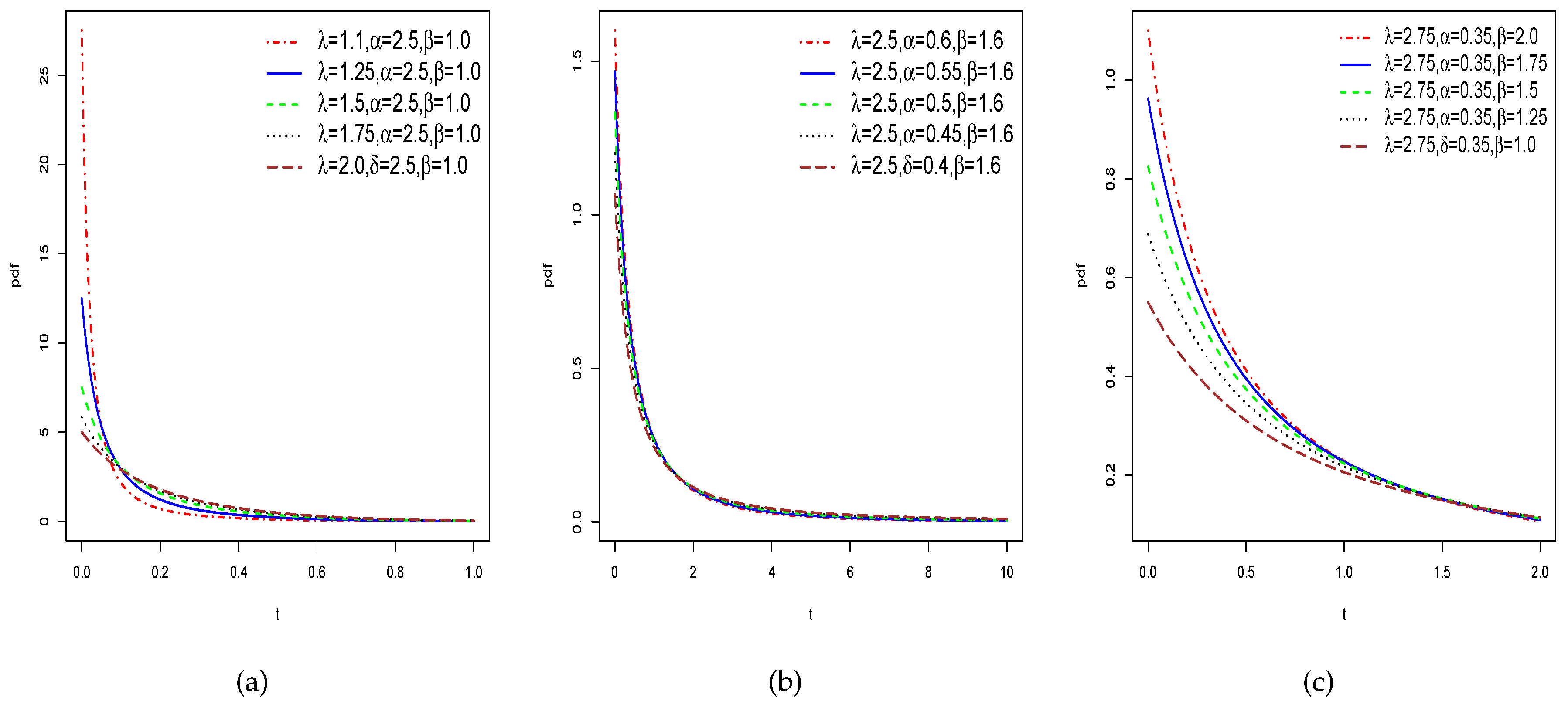
Figure 2.
cdf and sf plots of the HTNH model using different parameter values of .
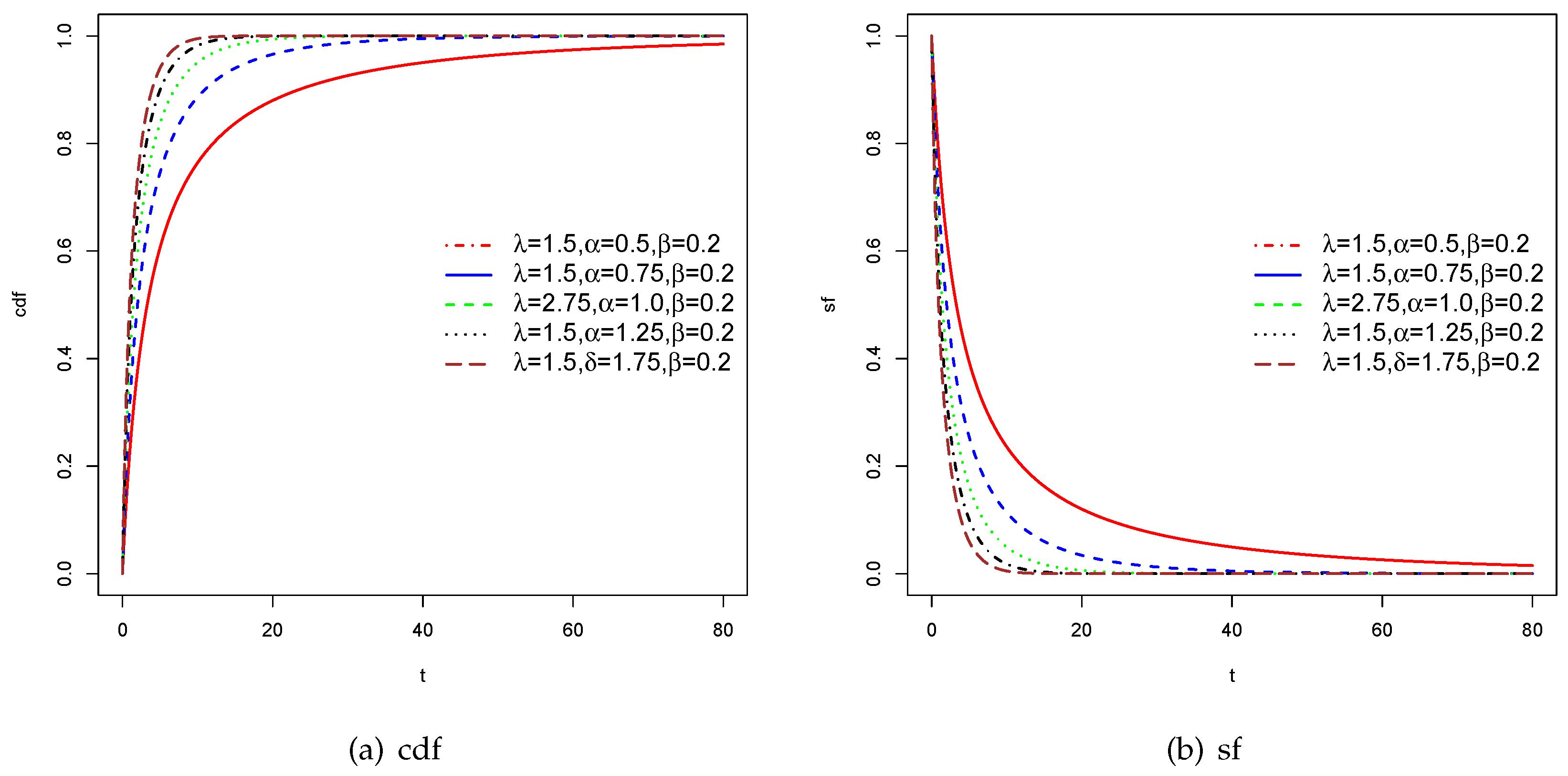
Figure 3.
hrf plots of the HTNH model using different parameter values of .
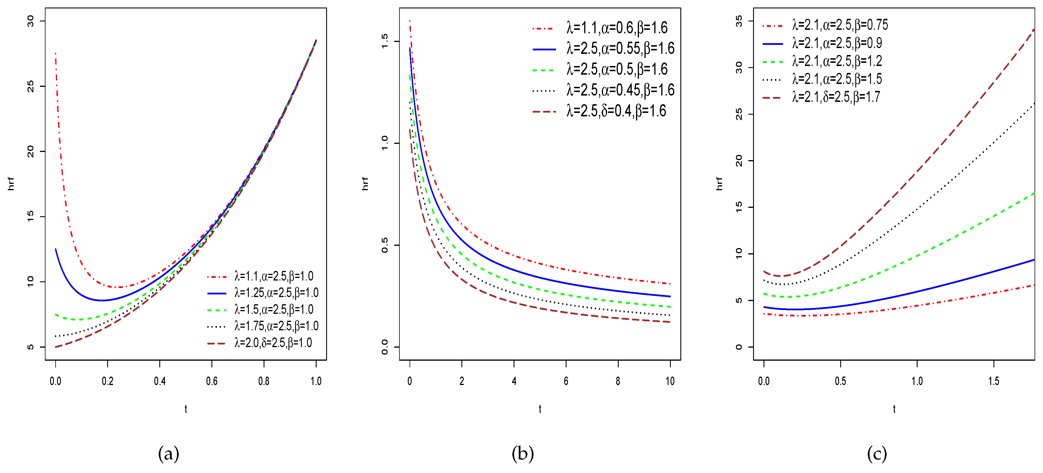
Figure 4.
3D curves for the proposed statistical properties of HTNH model at .
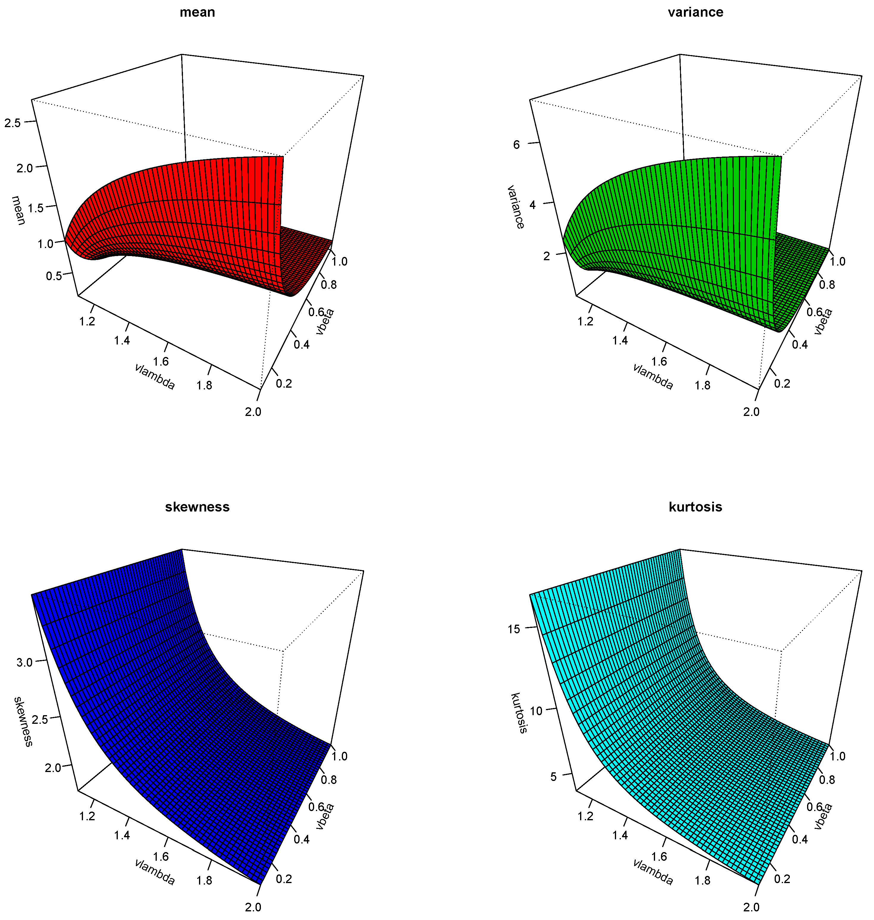
Figure 5.
3D curves for the proposed statistical properties of HTNH model at .
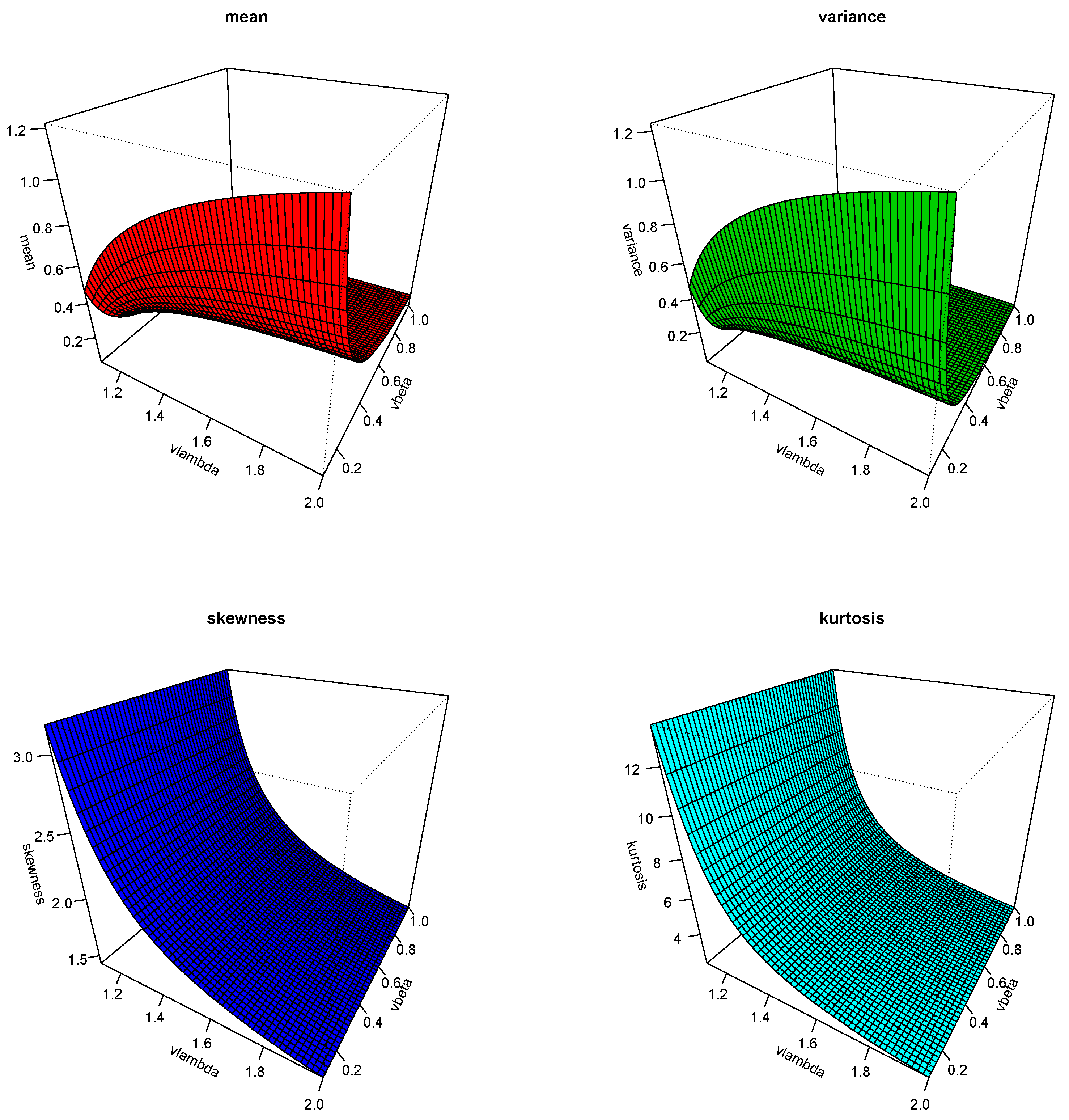
Figure 6.
3D curves of proposed entropy measures at and .
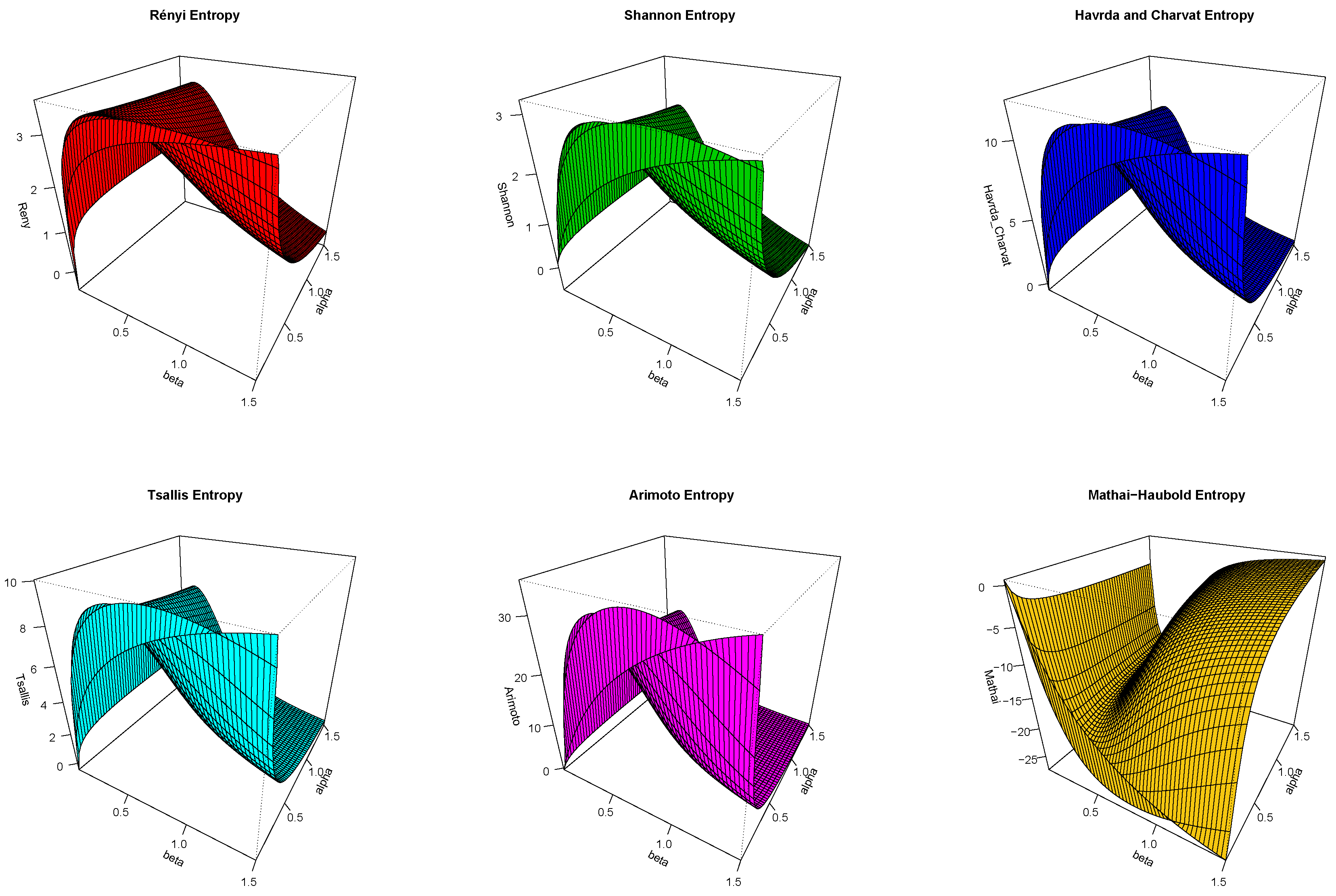
Figure 7.
3D curves of proposed entropy measures at and .
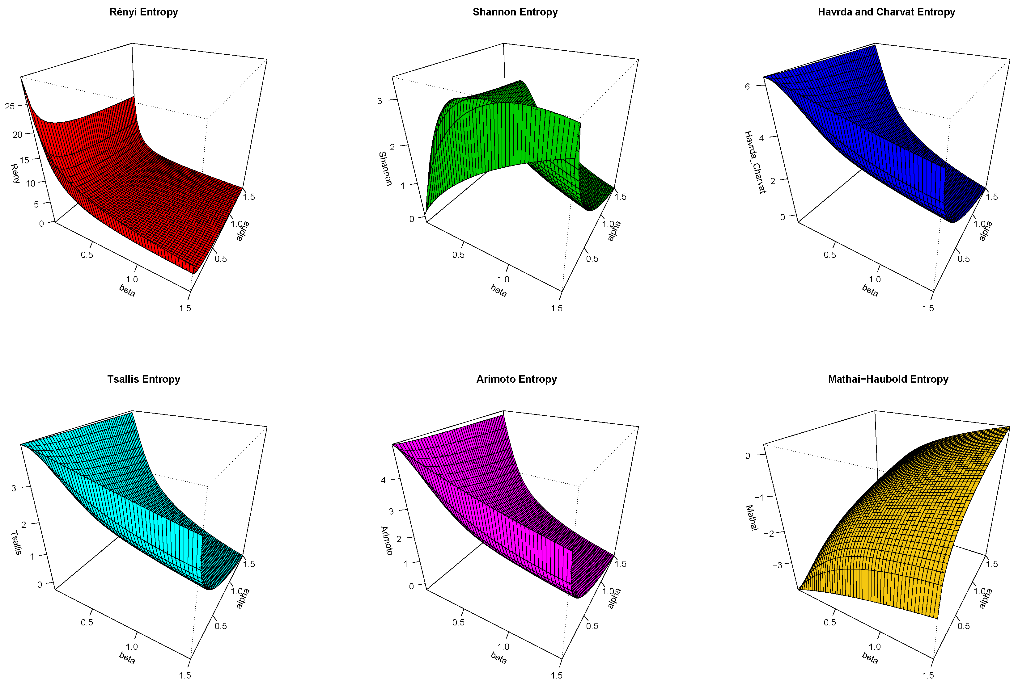
Figure 8.
Kernel density, TTT and box plots of the proposed three datasets.
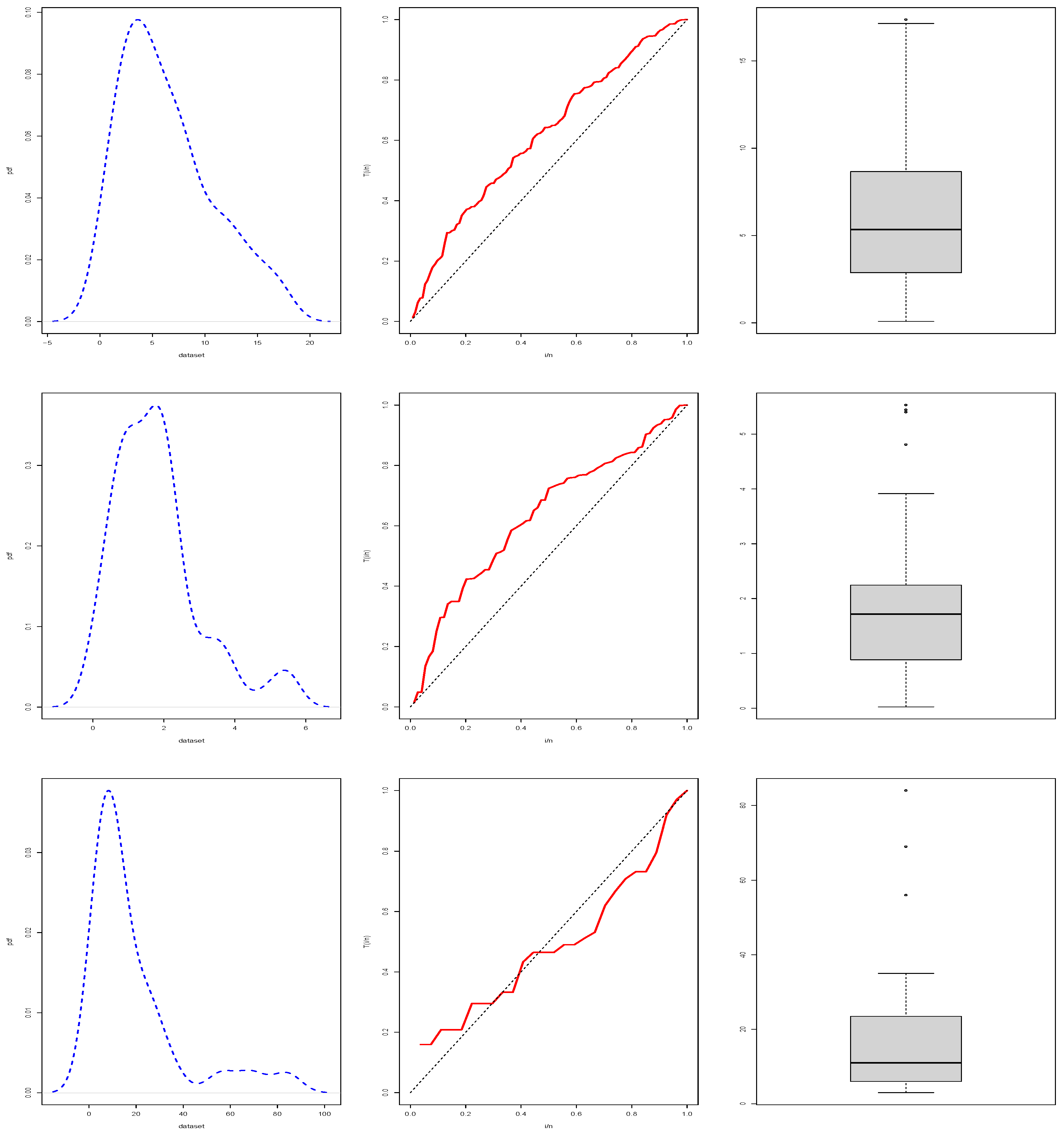
Figure 9.
Estimation plots of pdf and cdf of the fitting distributions using first dataset.
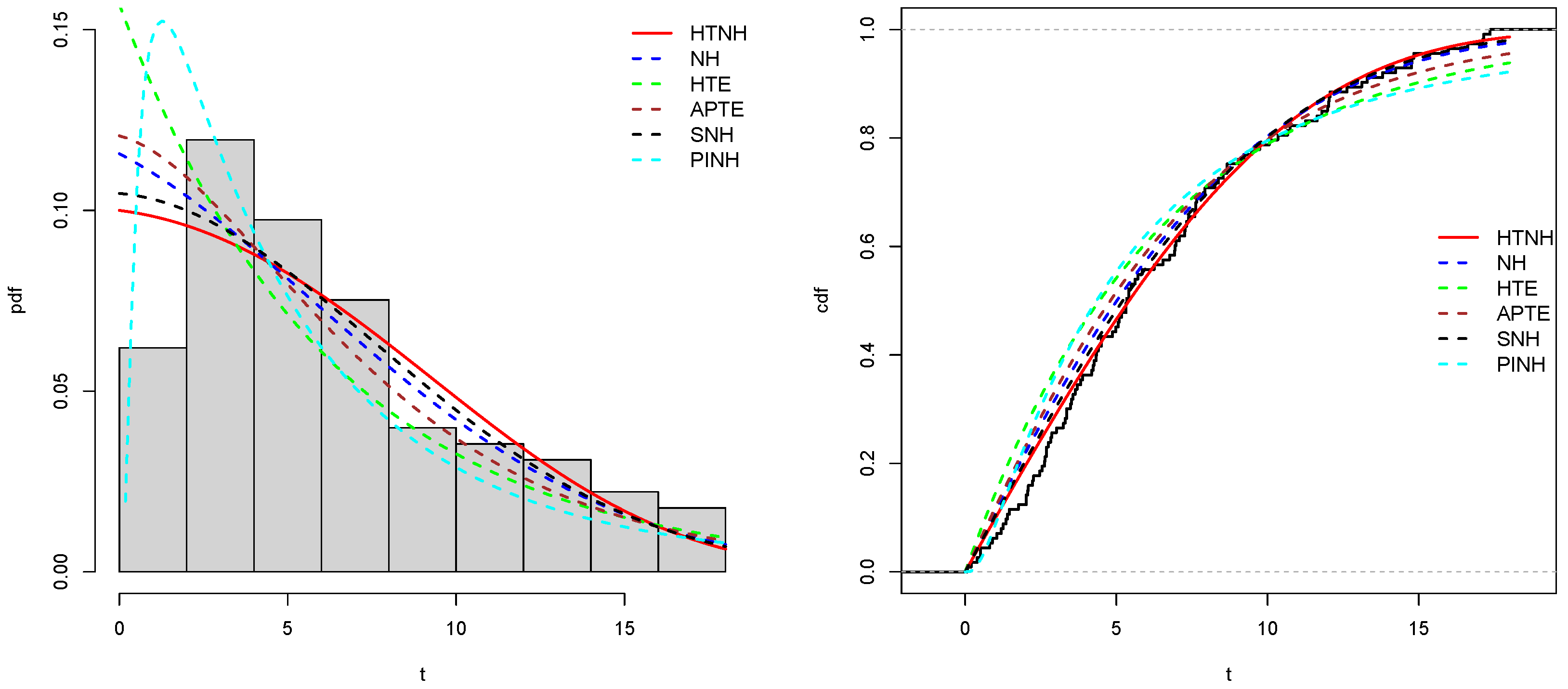
Figure 10.
Estimation plots of pdf and cdf of the fitting distributions using second dataset.
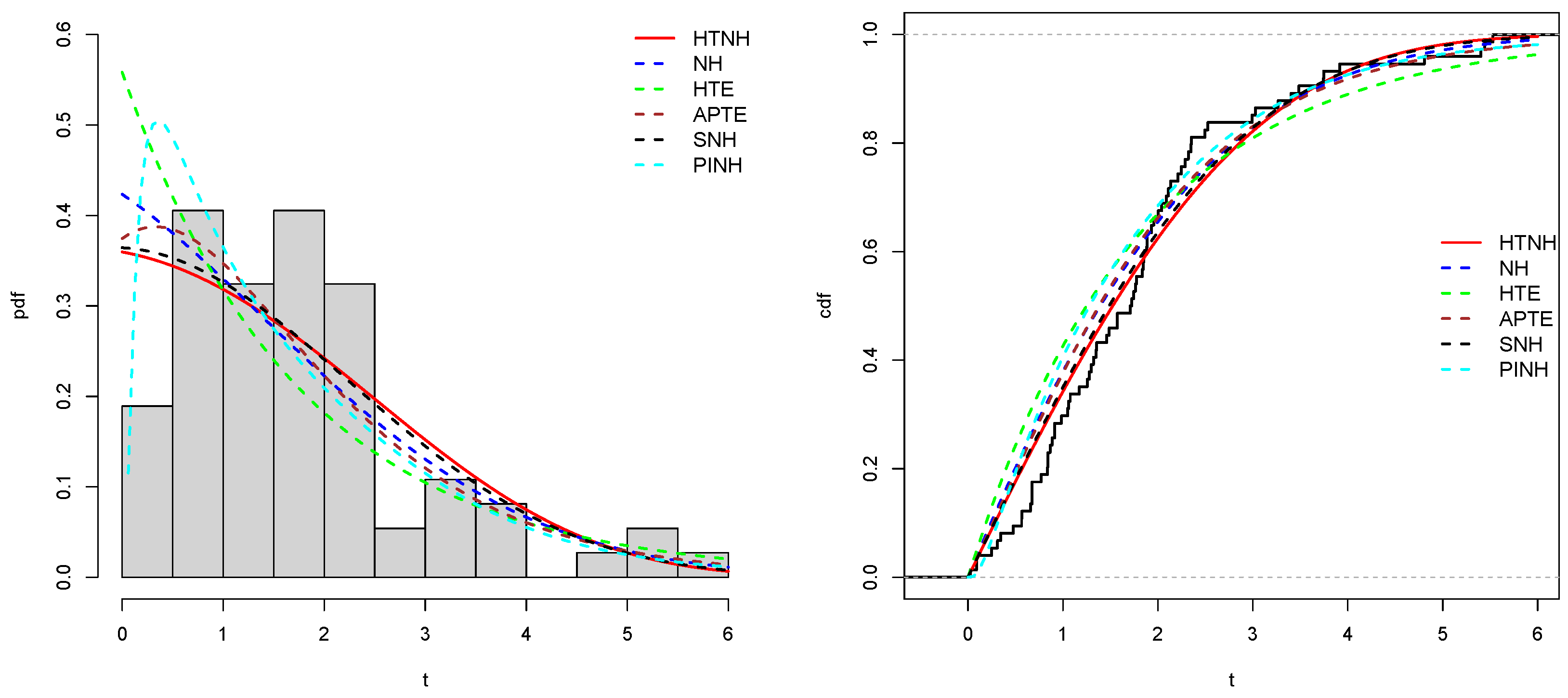
Figure 11.
Estimation plots of pdf and cdf of the fitting distributions using third dataset.
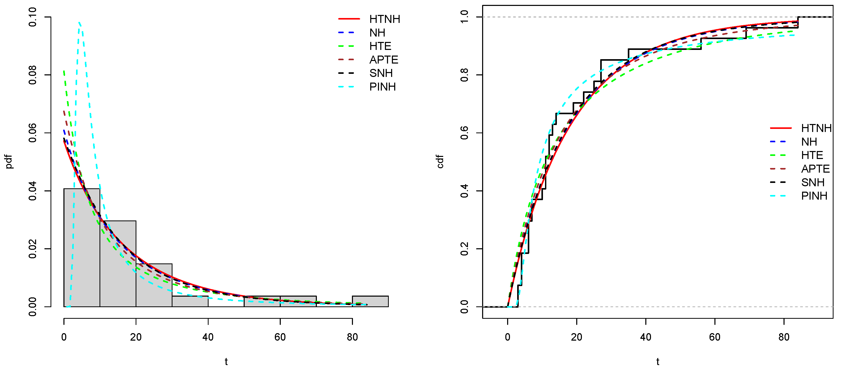
Table 1.
Numerous statistical measures for the HTNH model at .
| ID | |||||
| =2 0.2 | 1.3647 | 1.8501 | 1.3557 | 1.7282 | 3.6433 |
| 0.4 | 0.6823 | 0.4625 | 0.6778 | 1.7282 | 3.6433 |
| 0.6 | 0.4549 | 0.2056 | 0.4519 | 1.7282 | 3.6433 |
| 0.8 | 0.3412 | 0.1156 | 0.3389 | 1.7282 | 3.6433 |
| =3 0.2 | 1.5724 | 2.1078 | 1.3405 | 1.5172 | 2.7109 |
| 0.4 | 0.7862 | 0.5270 | 0.6703 | 1.5172 | 2.7109 |
| 0.6 | 0.5241 | 0.2342 | 0.4468 | 1.5172 | 2.7109 |
| 0.8 | 0.3931 | 0.1317 | 0.3351 | 1.5172 | 2.7109 |
| =4 0.2 | 1.6627 | 2.2149 | 1.3321 | 1.4361 | 2.3869 |
| 0.4 | 0.8314 | 0.5537 | 0.6661 | 1.4361 | 2.3869 |
| 0.6 | 0.5542 | 0.2461 | 0.4440 | 1.4361 | 2.3869 |
| 0.8 | 0.4157 | 0.1384 | 0.3330 | 1.4361 | 2.3869 |
Table 2.
Numerous statistical measures for the HTNH model at .
| ID | |||||
| =2 0.2 | 0.6127 | 0.3156 | 0.5151 | 1.4198 | 2.1529 |
| 0.4 | 0.3063 | 0.0789 | 0.2576 | 1.4198 | 2.1529 |
| 0.6 | 0.2042 | 0.0351 | 0.1717 | 1.4198 | 2.1529 |
| 0.8 | 0.1532 | 0.0197 | 0.1288 | 1.4198 | 2.1529 |
| =3 0.2 | 0.7014 | 0.3564 | 0.5082 | 1.2194 | 1.3991 |
| 0.4 | 0.3507 | 0.0891 | 0.2541 | 1.2194 | 1.3991 |
| 0.6 | 0.2338 | 0.0396 | 0.1694 | 1.2194 | 1.3991 |
| 0.8 | 0.1753 | 0.0223 | 0.1271 | 1.2194 | 1.3991 |
| =4 0.2 | 0.7395 | 0.3718 | 0.5028 | 1.1427 | 1.1605 |
| 0.4 | 0.3697 | 0.0929 | 0.2514 | 1.1427 | 1.1605 |
| 0.6 | 0.2465 | 0.0413 | 0.1676 | 1.1427 | 1.1605 |
| 0.8 | 0.1849 | 0.0232 | 0.1257 | 1.1427 | 1.1605 |
Table 3.
Different numerical records of proposed entropy measures at and .
| =1 0.2 | 3.0866 | 2.2944 | 8.8843 | 7.3600 | 20.9023 | -18.2487 |
| 0.4 | 2.7092 | 1.7463 | 6.9416 | 5.7506 | 14.0179 | -13.2577 |
| 0.6 | 1.9997 | 1.1071 | 4.1473 | 3.4358 | 6.3869 | -6.9614 |
| 0.8 | 1.3829 | 0.6686 | 2.4060 | 1.9932 | 2.9864 | -3.6424 |
| =2 0.2 | 2.9204 | 1.9489 | 7.9834 | 6.6136 | 17.5486 | -15.8757 |
| 0.4 | 2.2667 | 1.1079 | 5.0845 | 4.2121 | 8.6477 | -8.9483 |
| 0.6 | 1.3250 | 0.4178 | 2.2685 | 1.8793 | 2.7622 | -3.4027 |
| 0.8 | 0.6882 | -0.0192 | 0.9916 | 0.8215 | 0.9902 | -1.3512 |
| =3 0.2 | 2.8067 | 1.7044 | 7.4088 | 6.1376 | 15.5552 | -14.4146 |
| 0.4 | 1.9620 | 0.7159 | 4.0248 | 3.3342 | 6.1135 | -6.7115 |
| 0.6 | 0.9200 | 0.0168 | 1.4100 | 1.1681 | 1.5092 | -1.9874 |
| 0.8 | 0.2812 | -0.4180 | 0.3645 | 0.3019 | 0.3247 | -0.4696 |
Table 4.
Different numerical records of proposed entropy measures at and .
| =1 0.2 | 4.0285 | 2.5078 | 3.9894 | 2.5389 | 2.7661 | -2.1206 |
| 0.4 | 2.1733 | 2.3272 | 2.6347 | 1.6768 | 1.7626 | -1.3387 |
| 0.6 | 1.4374 | 1.6300 | 1.8973 | 1.2075 | 1.2493 | -0.9450 |
| 0.8 | 0.9841 | 1.1330 | 1.3707 | 0.8724 | 0.8933 | -0.6740 |
| =2 0.2 | 3.1994 | 2.3623 | 3.4607 | 2.2024 | 2.3632 | -1.8045 |
| 0.4 | 1.4736 | 1.7315 | 1.9368 | 1.2326 | 1.2763 | -0.9656 |
| 0.6 | 0.7493 | 0.9386 | 1.0736 | 0.6833 | 0.6958 | -0.5243 |
| 0.8 | 0.2973 | 0.4418 | 0.4503 | 0.2865 | 0.2887 | -0.2169 |
| =3 0.2 | 2.7427 | 2.2202 | 3.1191 | 1.9850 | 2.1111 | -1.6082 |
| 0.4 | 1.0705 | 1.3473 | 1.4758 | 0.9392 | 0.9637 | -0.7274 |
| 0.6 | 0.3488 | 0.5347 | 0.5249 | 0.3340 | 0.3369 | -0.2532 |
| 0.8 | -0.1017 | 0.0388 | -0.1619 | -0.1030 | -0.1028 | 0.0770 |
Table 5.
The AEs, ABs, and MSEs of the HTNH model using Case1.
| Simple size | Est. | ||||
| 300 | AE | 1.1693 | 0.2578 | 0.3750 | |
| AB | 0.0693 | 0.0078 | 0.1250 | ||
| MSE | 0.0406 | 0.0015 | 0.0961 | ||
| LCL | 1.0160 | 0.1850 | 0.0348 | ||
| UCL | 1.49699 | 0.34430 | 0.8798 | ||
| AL | 0.48096 | 0.1592 | 0.8450 | ||
| 500 | AE | 1.1185 | 0.2540 | 0.2754 | |
| AB | 0.0185 | 0.0040 | 0.0254 | ||
| MSE | 0.0091 | 0.0009 | 0.0303 | ||
| LCL | 1.0329 | 0.2034 | 0.0749 | ||
| UCL | 1.3272 | 0.3122 | 0.7323 | ||
| AL | 0.2942 | 0.1087 | 0.6573 | ||
| 700 | AE | 1.1066 | 0.2490 | 0.2671 | |
| AB | 0.0066 | 0.0009 | 0.0171 | ||
| MSE | 0.0032 | 0.0004 | 0.0193 | ||
| LCL | 1.0255 | 0.2096 | 0.0609 | ||
| UCL | 1.2568 | 0.2918 | 0.5987 | ||
| AL | 0.2312 | 0.0821 | 0.5378 | ||
| 1000 | AE | 1.1140 | 0.2521 | 0.2768 | |
| AB | 0.0140 | 0.0021 | 0.0268 | ||
| MSE | 0.0028 | 0.0004 | 0.0118 | ||
| LCL | 1.0385 | 0.2189 | 0.0778 | ||
| UCL | 1.2872 | 0.2932 | 0.5797 | ||
| AL | 0.2486 | 0.0743 | 0.5018 |
Table 6.
The AEs, ABs, and MSEs of the HTNH model using Case2.
| Simple size | Est. | ||||
| 300 | AE | 1.3907 | 0.2564 | 0.7021 | |
| AB | 0.1907 | 0.0064 | 0.2021 | ||
| MSE | 0.4052 | 0.0008 | 0.3405 | ||
| LCL | 1.0382 | 0.2130 | 0.0958 | ||
| UCL | 2.7006 | 0.3201 | 2.4076 | ||
| AL | 1.6623 | 0.1071 | 2.3118 | ||
| 500 | AE | 1.2729 | 0.2526 | 0.5977 | |
| AB | 0.0729 | 0.0026 | 0.0977 | ||
| MSE | 0.0502 | 0.0004 | 0.1159 | ||
| LCL | 1.0664 | 0.2183 | 0.1743 | ||
| UCL | 1.9156 | 0.2925 | 1.4563 | ||
| AL | 0.8491 | 0.0742 | 1.2819 | ||
| 700 | AE | 1.2412 | 0.2500 | 0.5632 | |
| AB | 0.0412 | 0.0009 | 0.0632 | ||
| MSE | 0.0357 | 0.0003 | 0.0990 | ||
| LCL | 1.0809 | 0.2173 | 0.2124 | ||
| UCL | 1.7205 | 0.2906 | 1.2128 | ||
| AL | 0.6396 | 0.0732 | 1.0003 | ||
| 1000 | AE | 1.2234 | 0.2485 | 0.5482 | |
| AB | 0.0234 | 0.0014 | 0.0482 | ||
| MSE | 0.0112 | 0.0001 | 0.0499 | ||
| LCL | 1.0876 | 0.2229 | 0.2304 | ||
| UCL | 1.5196 | 0.2730 | 1.1347 | ||
| AL | 0.4319 | 0.0501 | 0.9043 |
Table 7.
The AEs, ABs, and MSEs of the HTNH model using model using Case3.
| Simple size | Est. | ||||
| 300 | AE | 1.5444 | 0.1998 | 0.8704 | |
| AB | 0.1444 | 0.0001 | 0.1204 | ||
| MSE | 0.2738 | 0.0004 | 0.2116 | ||
| LCL | 1.1726 | 0.1767 | 0.3458 | ||
| UCL | 2.9200 | 0.2257 | 2.0828 | ||
| AL | 1.7474 | 0.0490 | 1.7360 | ||
| 500 | AE | 1.48077 | 0.2042 | 0.7789 | |
| AB | 0.0807 | 0.0042 | 0.0289 | ||
| MSE | 0.1231 | 0.0003 | 0.1334 | ||
| LCL | 1.1843 | 0.18292 | 0.3564 | ||
| UCL | 2.1959 | 0.2296 | 1.5652 | ||
| AL | 1.0115 | 0.0466 | 1.2088 | ||
| 700 | AE | 1.4606 | 0.2006 | 0.8202 | |
| AB | 0.0606 | 0.0006 | 0.0702 | ||
| MSE | 0.0493 | 0.0002 | 0.0981 | ||
| LCL | 1.2300 | 0.1848 | 0.4369 | ||
| UCL | 1.9319 | 0.2190 | 1.4832 | ||
| AL | 0.7019 | 0.0342 | 1.0462 | ||
| 1000 | AE | 1.4503 | 0.2002 | 0.8179 | |
| AB | 0.0503 | 0.0002 | 0.0679 | ||
| MSE | 0.0332 | 0.0001 | 0.0744 | ||
| LCL | 1.2239 | 0.1861 | 0.4696 | ||
| UCL | 1.8541 | 0.2163 | 1.4488 | ||
| AL | 0.6308 | 0.0302 | 0.9792 |
Table 8.
The AEs, ABs, and MSEs of the HTNH model using Case4.
| Simple size | Est. | ||||
| 300 | AE | 1.7282 | 0.2018 | 1.1295 | |
| AB | 0.1282 | 0.0018 | 0.1295 | ||
| MSE | 0.2834 | 0.0006 | 0.2045 | ||
| LCL | 1.2100 | 0.1708 | 0.3726 | ||
| UCL | 3.2956 | 0.2301 | 2.0673 | ||
| AL | 2.0856 | 0.0593 | 1.6947 | ||
| 500 | AE | 1.7273 | 0.2003 | 1.1062 | |
| AB | 0.1273 | 0.0003 | 0.1062 | ||
| MSE | 0.2051 | 0.0004 | 0.1678 | ||
| LCL | 1.2528 | 0.1829 | 0.5263 | ||
| UCL | 2.7325 | 0.2278 | 2.0077 | ||
| AL | 1.4797 | 0.0449 | 1.4814 | ||
| 700 | AE | 1.6982 | 0.1999 | 1.0477 | |
| AB | 0.0982 | 0.0001 | 0.0477 | ||
| MSE | 0.2316 | 0.0002 | 0.1696 | ||
| LCL | 1.2841 | 0.1843 | 0.4820 | ||
| UCL | 2.7068 | 0.2185 | 1.9236 | ||
| AL | 1.4227 | 0.0342 | 1.4615 | ||
| 1000 | AE | 1.6350 | 0.1991 | 1.0195 | |
| AB | 0.0350 | 0.0008 | 0.0195 | ||
| MSE | 0.0829 | 0.0001 | 0.0921 | ||
| LCL | 1.3273 | 0.18282 | 0.6125 | ||
| UCL | 2.4934 | 0.2126 | 1.7508 | ||
| AL | 1.1661 | 0.0297 | 1.1383 |
Table 12.
Summary statistic measures for the three considered datasets.
| Dataset | Median | Mean | ID | ||||
| 1 | 2.870 | 5.340 | 6.408 | 8.660 | 3.012 | 0.738 | -0.312 |
| 2 | 0.891 | 1.717 | 1.801 | 2.237 | 0.851 | 1.196 | 1.3517 |
| 3 | 6.000 | 11.000 | 18.810 | 23.500 | 22.355 | 1.846 | 2.610 |
Table 13.
Parameter estimations with various statistic comparison measures for the two considered datasets.
Table 13.
Parameter estimations with various statistic comparison measures for the two considered datasets.
| Dataset | Model | -value | |||||||
|---|---|---|---|---|---|---|---|---|---|
| HTNH | 32.327 | 17.255 | 0.0056 | 0.0743 | 0.5596 | -312.774 | 631.549 | 639.732 | |
| PINH | 0.2289 | 218.607 | 2.1747 | 0.1273 | 0.0512 | -328.966 | 663.932 | 672.114 | |
| NH | 2.7633 | 0.0418 | 0.0983 | 0.2239 | -318.406 | 640.825 | 646.280 | ||
| I | HTE | 53.497 | 0.1540 | 0.1472 | 0.0149 | -323.134 | 650.268 | 650.377 | |
| SNH | 1.1934 | 0.0702 | 0.1212 | 0.0723 | -318.628 | 641.272 | 646.727 | ||
| APTE | 0.1955 | 2.4602 | 0.1100 | 0.1297 | -319.784 | 642.918 | 648.372 | ||
| HTNH | 37.658 | 9.2309 | 0.0379 | 0.1081 | 0.3289 | -111.694 | 229.388 | 236.300 | |
| PINH | 0.1176 | 235.45 | 4.0355 | 0.1544 | 0.0524 | -116.978 | 239.956 | 246.868 | |
| NH | 2.3901 | 0.1771 | 0.1381 | 0.1077 | -114.485 | 232.970 | 237.578 | ||
| II | HTE | 50.236 | 0.5470 | 0.1844 | 0.0112 | -117.712 | 239.424 | 244.032 | |
| SNH | 1.5596 | 0.1815 | 0.1493 | 0.0661 | -115.357 | 234.714 | 239.322 | ||
| APTE | 0.7621 | 3.6160 | 0.1302 | 0.1488 | -114.203 | 232.406 | 237.014 | ||
| HTNH | 13.359 | 0.9402 | 0.0562 | 0.1561 | 0.5257 | -106.209 | 218.418 | 222.306 | |
| PINH | 51.976 | 0.0899 | 0.9757 | 0.1605 | 0.4897 | -106.214 | 218.428 | 222.315 | |
| NH | 0.8113 | 0.0750 | 0.1640 | 0.4620 | -111.238 | 226.476 | 229.067 | ||
| III | HTE | 1.3786 | 0.0223 | 0.2013 | 0.2235 | -113.421 | 230.842 | 233.433 | |
| SNH | 0.6403 | 0.0577 | 0.1598 | 0.4853 | -108.696 | 221.392 | 223.983 | ||
| APTE | 0.0297 | 0.1434 | 0.1784 | 0.3565 | -112.401 | 228.802 | 231.393 |
Disclaimer/Publisher’s Note: The statements, opinions and data contained in all publications are solely those of the individual author(s) and contributor(s) and not of MDPI and/or the editor(s). MDPI and/or the editor(s) disclaim responsibility for any injury to people or property resulting from any ideas, methods, instructions or products referred to in the content. |
© 2024 by the authors. Licensee MDPI, Basel, Switzerland. This article is an open access article distributed under the terms and conditions of the Creative Commons Attribution (CC BY) license (http://creativecommons.org/licenses/by/4.0/).
Copyright: This open access article is published under a Creative Commons CC BY 4.0 license, which permit the free download, distribution, and reuse, provided that the author and preprint are cited in any reuse.


