Submitted:
30 June 2025
Posted:
02 July 2025
You are already at the latest version
Abstract
This study employs advanced geospatial analysis and information-theoretic modeling to evaluate the relationship between multi-scale vegetation patterns, temporal change, and wildfire size over 19 ecoregions in the western United States. More specifically, the study quantifies and extends established understanding about the relationship between vegetation patterns and fire behavior while demonstrating how information-theoretic modeling and GIS data can provide quantitative insights into complex spatiotemporal relationships. Using a custom-developed concentric ring buffer aggregation approach, we extracted vegetation characteristics from National Land Cover Database (NLCD) rasters at three nested spatial scales around the 2015 to 2020 wildfire ignition points: an inner ring (0-90m from ignition), middle ring (90-150m from ignition), and outer ring (150-210m from ignition) at the 30m resolution of the NLCD data. The entire yearly land cover raster catalog from 1985 to 2020 was sampled using this algorithm in five year increments. This results in a 30-year record for each fire, consisting of the most common land cover in each ring, for each 5 year increment, for a total of 7 time samples per fire. Categorical data from these spatiotemporal lags were analyzed using Variable-Based Reconstructability Analysis (VB-RA), an information-theoretic modeling framework that identifies statistically significant structural relationships among categorical variables. Our analysis reveals that vegetation that has developed for 15 to 30 years is a strong predictor of larger fires, as measured by the overall size of final destruction, not by other metrics such as destruction of buildings or severity. Grassland and shrubland dominance, particularly older, well-established vegetation, were consistently associated with large fires, The temporal consistency of vegetation patterns from 15 to 30 years appears particularly important, suggesting that stable grassland and shrubland configurations are highly predictive of large-sized fire events.
Keywords:
geospatial modeling
; categorical data analysis
; information theory
; reconstructability analysis
; wildfire behavior
; land cover classification
; multi-scale spatial analysis
; vegetation dynamics
; ring buffer analysis
; GIS raster analysis
; fire ignition modeling
; entropy
; spatial neighborhood patterns
; landscape metrics
; NLCD classification
1. Introduction
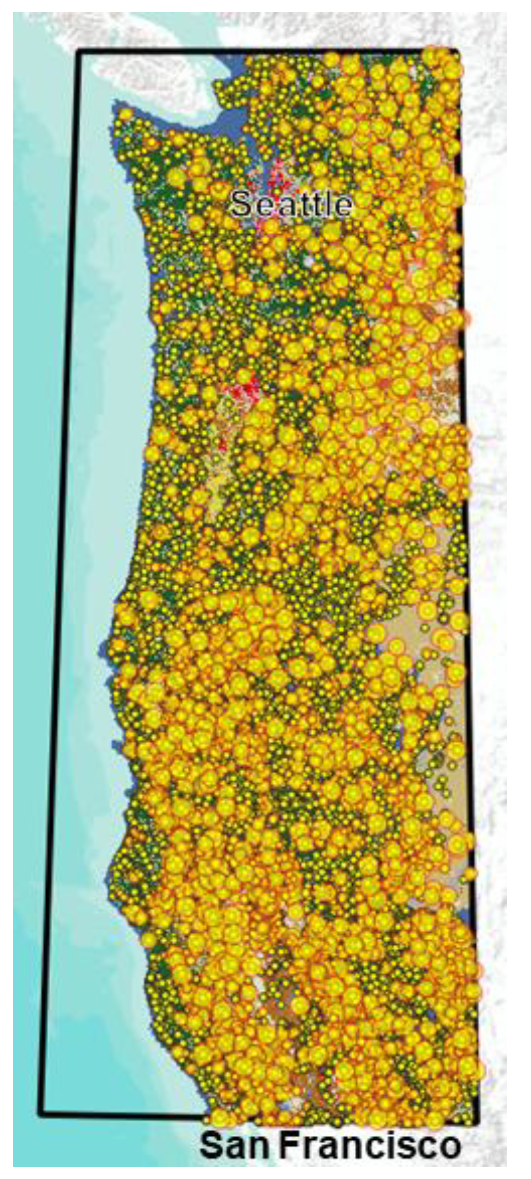
Wildfires have become an increasingly dominant force shaping landscapes across the western United States. In recent decades, the size, intensity, and frequency of large wildfire events have surged (Abatzoglou and Williams, 2016; Westerling, 2016), creating urgent challenges for land management agencies, policymakers, and ecological conservation efforts. While climatic trends (Abatzoglou and Williams, 2016) and topographic features are well-established drivers of fire behavior, a critical yet understudied factor is the role of local vegetation structure immediately surrounding ignition points. How vegetation patterns, both current and historical, influence whether an ignition grows into a large, destructive wildfire remain vital and actionable research questions. GIS data that provide a historical record of land use can help answer these questions, and machine learning can find the patterns. This paper will show that Reconstructability Analysis, a categorical data machine learning methodology based in information theory, can identify and quantify the factors that predict large as opposed to small wildfires. Additionally, we introduce a spatial aggregation technique using concentric ring buffers. We will also identify some places that meet criteria for extreme risk, as predicted by our models. The study area, shown in Figure 1, is a swath of the West Coast of the USA encompassing the researchers’ home, and prone to large wildfires. It consists of 19 ecoregions referred to as “pyromes” in the fire science literature.
Reconstructability Analysis
Reconstructability Analysis (RA) is a powerful modeling paradigm that offers a transparent, information-theoretic framework for uncovering structural patterns among categorical variables (Zwick, 2004). Unlike conventional approaches, RA naturally accommodates categorical data while producing highly interpretable models organized in a systematic lattice structure. See Methods section 2.4.1 for RA details.
Study Objectives
This study addresses a knowledge gap by investigating the predictive power of surrounding land cover in determining eventual wildfire size. Specifically, we leverage a categorical, ring-buffer-based analysis of ignition points using land cover classifications (Figure 2) from the National Land Cover Database (NLCD) and ignition records from the Fire Program Analysis Fire Occurrence Database (FPA FOD). Fires ignited between 2015 & 2020 were classified into “small” (Classes A and B, <10 acres) and “large” (Classes C through G, ≥10 acres) categories, providing a binary framework for predictive (classifier) modeling. Figure 3 shows the spatial distribution of large & small fires, while Figure 6 shows the fire size distribution.
Figure 2.
National Land Cover codes & descriptions used in NLCD database, colors are used throughout this paper. Codes 11, 12, 21 – 24, 31, 90, & 95 are grouped in this study, leaving an 8 class set of NLCD classifications to analyze.
Figure 2.
National Land Cover codes & descriptions used in NLCD database, colors are used throughout this paper. Codes 11, 12, 21 – 24, 31, 90, & 95 are grouped in this study, leaving an 8 class set of NLCD classifications to analyze.
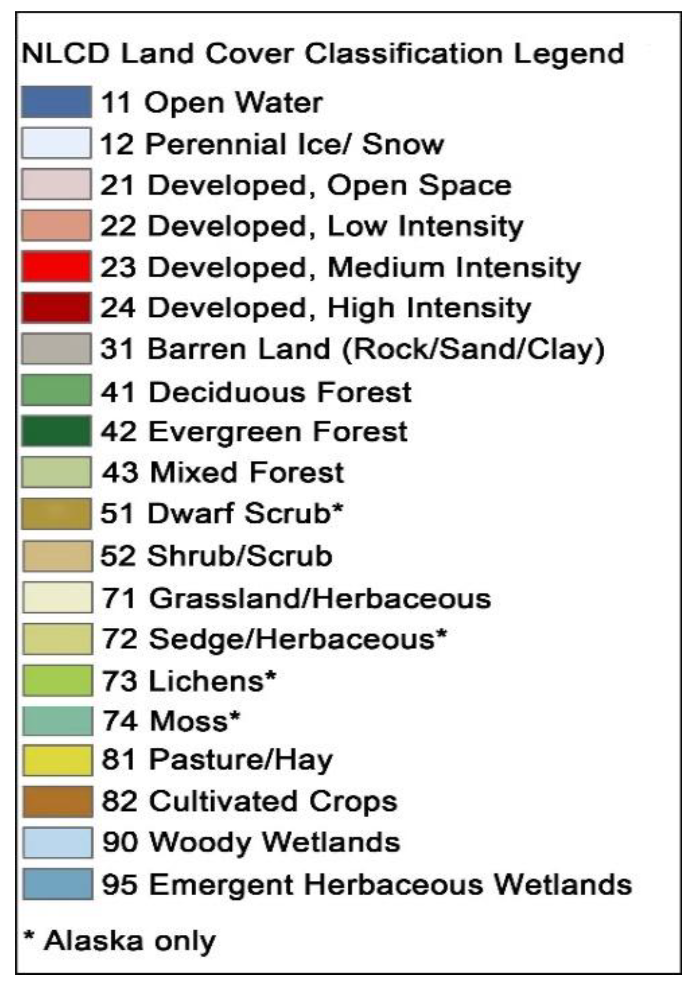
Our approach synthesizes medium resolution spatial analysis with categorical multivariate modeling. We extract dominant vegetation types within concentric rings around each ignition point at seven temporal layers (1985 through 2020), enabling us to capture both contemporary vegetation conditions and long-term landscape legacy effects. Employing Variable-Based Reconstructability Analysis (VB-RA) allows us to model complex categorical interactions with high interpretability and minimal risk of overfitting. Our primary objective is to discern whether the age of certain vegetation patterns—specifically, the highly flammable types like grasslands and shrublands (Balch et al., 2013)—are systematically associated with a greater likelihood of fire escalation to large areas and, if so, how.
Through this analysis, we aim to quantify well-established relationships between vegetation patterns and fire behavior using a novel analytical approach. We are not here claiming to discover new wildfire causes; rather, our contribution lies in the application of information-theoretic methods to confirm and quantify relationships already partially understood by fire scientists, while providing a transparent and interpretable modeling framework. In a context where large wildfires have devastating ecological, economic, and social consequences (Stephens et al., 2014), identifying simple, spatially explicit predictors of fire escalation could play a critical role in prioritizing early response efforts and mitigating future fire risk.
2. Methods
This study conducts a detailed spatial and categorical modeling analysis focused on predicting the size of wildfires at wildfire ignition points from the 2015 to 2020 fire seasons. All geospatial preprocessing, feature extraction, and model construction steps are performed using open-source tools, such as QGIS for the desktop work and Rasterio for raster extraction, to ensure transparency and reproducibility. Tools developed in Python for this project are available on our Occam Github site (https://github.com/occam-ra/occam).
Figure 3.
Wildfires from 2015 -2020 symbolized by size with classes A & B shown as small yellow points, while large fires (C, D, E, F, &G) are large yellow circles with red outlines.
Figure 3.
Wildfires from 2015 -2020 symbolized by size with classes A & B shown as small yellow points, while large fires (C, D, E, F, &G) are large yellow circles with red outlines.
As noted earlier, the primary novelty of this work lies in the application of information-theoretic modeling to wildfire size prediction using historical data, not in discovering previously unknown fire causes. Reconstructability Analysis offers several advantages for this domain: (1) it naturally accommodates categorical data without transformation, (2) it produces highly interpretable models with explicit variable relationships, and (3) it quantifies information content and uncertainty (Shannon entropy) reduction in a statistically rigorous framework. These methodological strengths complement existing process-based and empirical wildfire models while offering a transparent alternative to ‘black box’ machine learning approaches.
2.1. GIS Data Preparation and Multi-Scale Spatial Processing
The geospatial analysis framework developed for this study required coordination of multi-temporal raster datasets with point-based ignition records across varied spatial and temporal scales. We designed and implemented a multi-scale spatial neighborhood analysis centered on wildfire ignition points from the 2015 to 2020 fire seasons, extracted from the Fire Program Analysis Fire Occurrence Database (FPA FOD). These points were used as the center of the raster extraction kernel that processed the data from the entire yearly stack of NLCD data (1985 to 2020), using a temporal kernel that samples every five years. All geospatial processing utilized the Albers Equal Area Conic projection (EPSG:5070) with North American Datum 1983 (NAD83) to ensure consistent coordinates across the western United States study region.
The cornerstone of our GIS methodology was the development of a hierarchical concentric ring buffer algorithm (Figure 4) that extracts land cover information at three distinct spatial scales around each ignition point. By “rings” at different spatial scales we mean nested squares of GIS raster data. This approach builds on our previous work applying information-theoretic neighborhood analysis to NLCD data (Percy and Zwick, 2024) but extends it to a multi-ring design centered on ignition points:
Figure 4.
- NLCD data overlaid with raster extraction “rings”. Colors correspond to standard NLCD legend of Figure 2. Large red dot represents the fire currently being processed. Cells are 30m, so the inner ring is 30 – 60m, middle ring is 90 – 120m, and outer is 150 – 180m.
Figure 4.
- NLCD data overlaid with raster extraction “rings”. Colors correspond to standard NLCD legend of Figure 2. Large red dot represents the fire currently being processed. Cells are 30m, so the inner ring is 30 – 60m, middle ring is 90 – 120m, and outer is 150 – 180m.
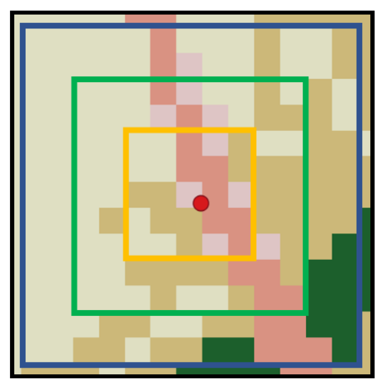
- Inner Ring: 3×3 and 5×5 pixel neighborhoods (30 – 60m), capturing immediate fuel conditions at the ignition site (Finney et al., 2005)
- Middle Ring: 7×7 and 9×9 pixel neighborhoods (90 – 120m), representing the zone where initial fire establishment typically occurs (Balch et al., 2013)
- Outer Ring: 11×11 and 13×13 pixel neighborhoods (150 – 180m), encompassing potential ember spotting distances and broader landscape context (Dillon et al., 2011; Westerling, 2016)
Within each ring, we identified both dominant and subdominant land cover classes based on raster cell frequency from seven NLCD land cover rasters at seven different times (T, T - 5, T - 10, T - 15, T - 20, T - 25, & T - 30), enabling us to capture both contemporary vegetation conditions and long-term landscape legacy effects (Bradley et al., 2018). Figure 5 illustrates the raster stack. The implementation for extracting a record of data for each fire is to encode the most common NLCD class for each ring in the current layer T (layer 0), and then do the same in five-year increments going back 30 years. Computing the most common (dominant) NLCD class will never result in a tie, since all of the rings have uneven numbers of cells (25 for the inner ring, 81 for the middle, and 169 for the outer). The second-most common class is called the sub-dominant, and in the case where the entire ring is occupied by all the same NLCD class we populate the sub-dominant field with the same dominant value to avoid holes in the database.
Figure 5.
Sample stack of National Landcover data from 1985 to 2015. Time 0 is the year of the fire being extracted; numbers associated with other times (years) are lags. For example, a fire from 2017 gets 3 ring data from years 2017 (T), 2012 (T-5), 2007 (T-10), 2002 (T-15), 1997 (T-20), 1992 (T-25), & 1987 (T-30).
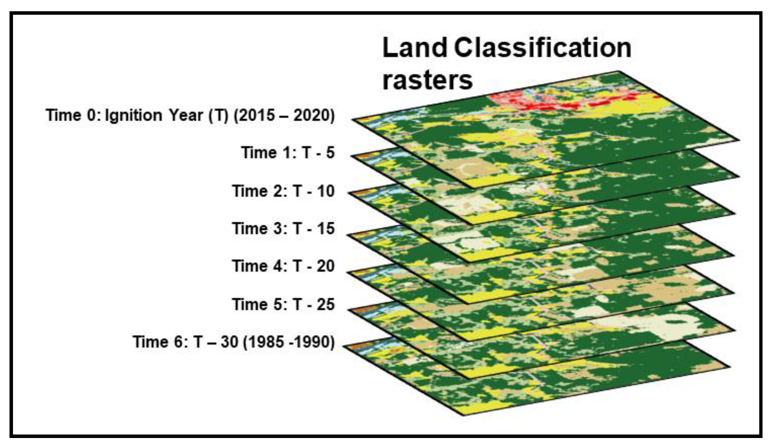
Multi-temporal Raster Processing and Standardization As seen in Figure 5, yearly NLCD land cover rasters (1985 through 2020) were acquired from the USGS MRLC site. After organizing into a local database, they were clipped to the study area and reprojected to the CRS used for the project (Albers Equal Area). At this point they were ready to be extracted. Extraction with our custom kernel produces a set of independent variables (IVs) that are in this form:
[Center_X, Center_X, Fire_ID, In_0_Dom, In_0_Sub, Mid_0_Dom, Mid_0_Sub, Out_0_dom, Out_0_sub, In_1_dom, In_1,_sub, Mid_1_dom, Mid_1_sub, Out_1_dom, Out_1_sub, etc,…Out_6_sub]
A total of 42 extracted NLCD codes for each fire were then joined to other data such as elevation and fires size based on the shared Fire_ID. Table 1 shows a complete listing of the variables extracted using the multi-ring extractor.

Table 1.
Extracted variables (IVs for our model) from the multi-ring extraction algorithm. Each fire from 2015 to 2020 had its location plotted on a continuous stack of NLCD data from 1985 to 2020, which was then sampled every five years for a total of 7 layers of data per fire. Within each layer, the inner, middle, and outer rings were sampled as shown in Figure 4, resulting in 42 NLCD codes per fire ignition.
| Time layer | Inner Ring Dominant & SubDominant | Middle Ring Dominant & SubDominant | Outer Ring Dominant & SubDominant |
| T- 0 (time of ignition) | In_0_Dom, In_0_Sub | Mid_0_Dom, Mid_0_Sub | Out_0_Dom, Out_0_Sub |
| T – 1 (5 year lag) | In_1_Dom, In_1_Sub | Mid_1_Dom, Mid_1_Sub | Out_1_Dom, Out_1_Sub |
| T – 2 (10 year lag | In_2_Dom, In_2_Sub | Mid_2_Dom, Mid_2_Sub | Out_2_Dom, Out_2_Sub |
| T – 3 (15 year lag) | In_3_Dom, In_3_Sub | Mid_3_Dom, Mid_3_Sub | Out_3_Dom, Out_3_Sub |
| T – 4 (20 year lag) | In_4_Dom, In_4_Sub | Mid_4_Dom, Mid_4_Sub | Out_4_Dom, Out_4_Sub |
| T – 5 (25 year lag) | In_5_Dom, In_5_Sub | Mid_5_Dom, Mid_5_Sub | Out_5_Dom, Out_5_Sub |
| T – 6 (30 year lag) | In_6_Dom, In_6_Sub | Mid_6_Dom, Mid_6_Sub | Out_6_Dom, Out_6_Sub |
Elevation, Ignition Cause, and Season Variables
In addition to the 42 ring extracted independent variables shown in Table 1 (two IVs for each cell in columns 2-4), elevation, ignition cause, and season were also used as IVs, Elevation values for fire ignition points were obtained from the FOD FPA. Elevation bins were subsequently defined based on these values to support categorical modeling within the Occam framework. The bins were chosen to maximize the maximize the information gain relative to predicting our target variable, and are [0-1500, 1500-2000, 2000-2500, 2500-3500, > 3500 meters]. Season was derived from the date of fire ignition, binned into Winter, Spring, Summer, and Fall. Unsurprisingly, the majority of large fires occur in the Summer. Ignition Cause was also added as an IV to the database from the FOD FPA, based on the NWCG general cause classifications.
2.2. Dependent Variable Construction
Wildfire size in this study is a binary DV with values “small” and “large.” Wildfire size classes are determined based on the final size recorded in the FPA FOD. As shown in Table 2 (and Figure 6), most fires were small. Fires less than 10 acres (Classes A and B) were classified as “small” in alignment with National Wildfire Coordinating Group (NWCG) operational standards (NWCG, 2020), while fires 10 acres or larger (Classes C-G) were classified as “large” (Finney et al., 2005; Stephens et al., 2014).
Table 2.
Number of Fires by Fire Class (2015 Ignitions).
| Fire Class | Size Range (Acres) | Number of Fires |
| A | 0–0.25 | 4,692 |
| B | 0.26–9.9 | 1,825 |
| C | 10–99 | 230 |
| D | 100–299 | 70 |
| E | 300–999 | 32 |
| F | 1,000–4,999 | 0 |
| G | ≥5,000 | 0 |
The binary classification of fire sizes provides a clear, operationally relevant dependent variable for our analysis. The threshold of 10 acres corresponds to a significant transition in fire management response, with larger fires typically requiring more extensive resources and often exhibiting qualitatively different fire behavior. This binarization also allows a balanced approach to the highly skewed distribution of fire sizes, which follows a classic power-law distribution as seen in many natural phenomena. Specifically, we balance the data set by randomly sampling an equal number of small fires to match the available number of large fires.
2.3. Pyrome Grouping
The study area consists of 19 different ecoregions that are known as pyromes in the fire science literature. This high cardinality (number of classes) is difficult to work with in information theoretic modelling, and needs to be grouped meaningfully. We employed a clustering technique on the pyromes by using the signatures from the 21-variable string of dominant NLCD codes. First, we binned the 15 NLCD classes down to 7 vegetation types, plus one class for all of the other developed, water, and barren codes, resulting in an 8-class model. Then, each of the 19 pyromes had a representative signature generated by calculating the mode (most frequent value) of each of the 21 binned NLCD values. These 19 signatures were then evaluated using a Hamming distance space (a sequence comparison algorithm), and clustered based on similarities. The silhouette plots showed that a five-cluster result was optimal, so the
pyromes were clustered into 5 groups as shown in Figure 7. Other groupings were attempted based on available ecosystem characteristics, such as precipitation, and predominant vegetation. Good reduction of uncertainty results were obtained from several other of these pyrome groupings, suggesting that the “signal” from the data with regard to predicting large fires is robust. The final choice to use this particular signature grouping mechanism, based on clustering, was due to the overall goodness of the reduction of uncertainty, %dH. As mentioned in section 2.2, we sampled the small fires to create a set that matches the number of large fires to balance the data for each pyrome group, so that each pyrome has an equal number of small and large fires.
Figure 6.
– Kernel Density illustration of fire size distribution. The bold line at 10 on the logarithmic X axis is the cutoff for small vs large fires in this study.
Figure 6.
– Kernel Density illustration of fire size distribution. The bold line at 10 on the logarithmic X axis is the cutoff for small vs large fires in this study.
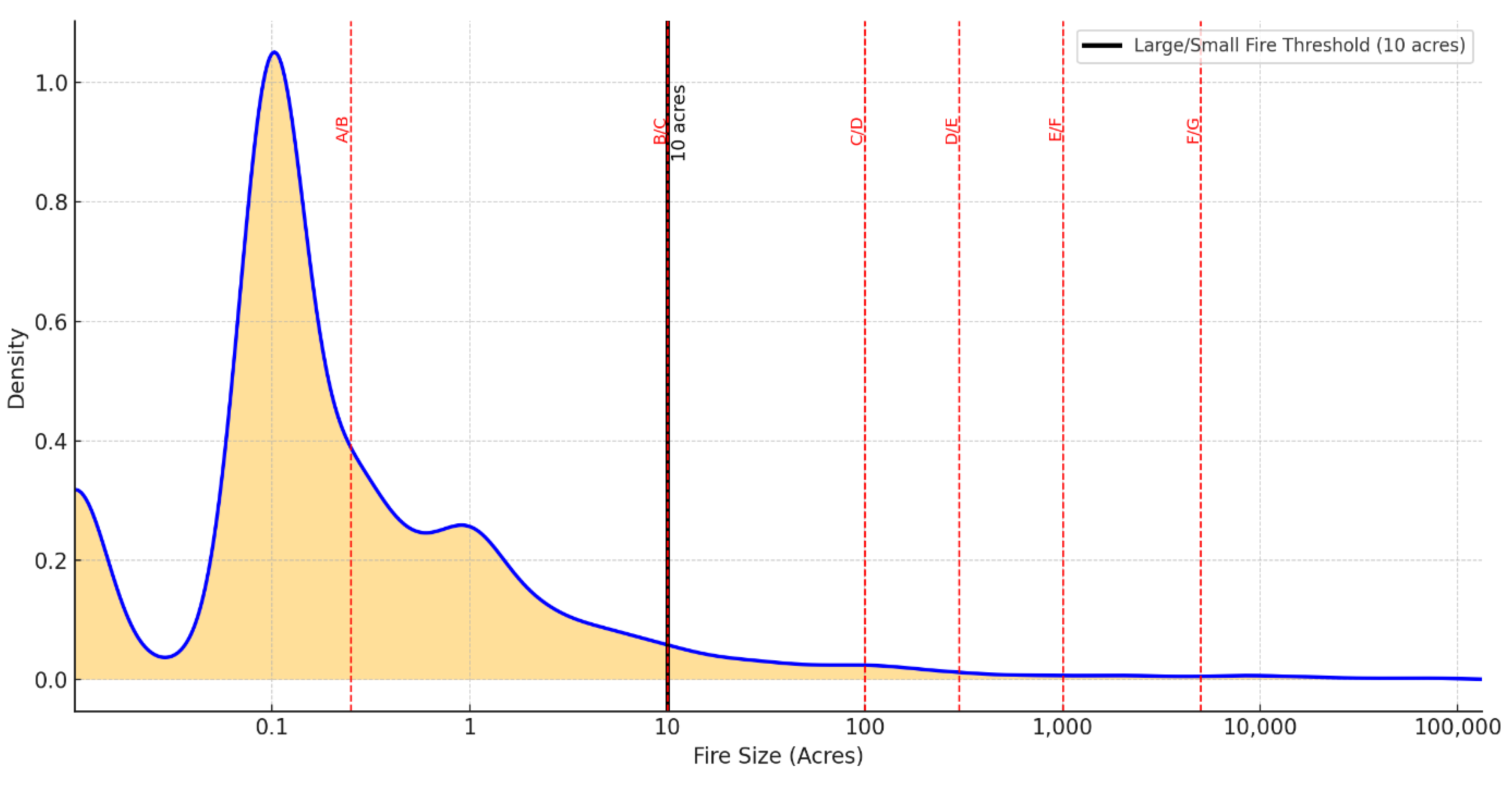
Figure 7.
Pyrome Groups: pyrome outlines are shown in gray, five signature groups are designated by color and labeled by letter. Pyrome signatures are generated by calculating the most common set of attribute values for each pyrome, and then clustering is based on these signatures.
Figure 7.
Pyrome Groups: pyrome outlines are shown in gray, five signature groups are designated by color and labeled by letter. Pyrome signatures are generated by calculating the most common set of attribute values for each pyrome, and then clustering is based on these signatures.
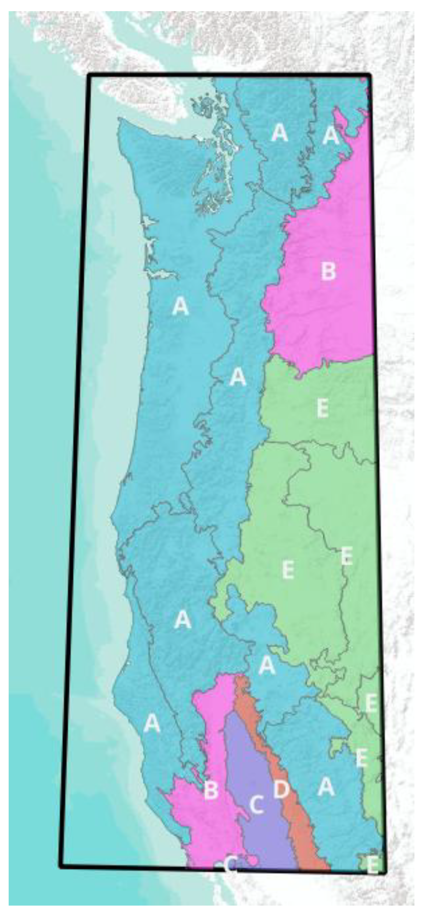
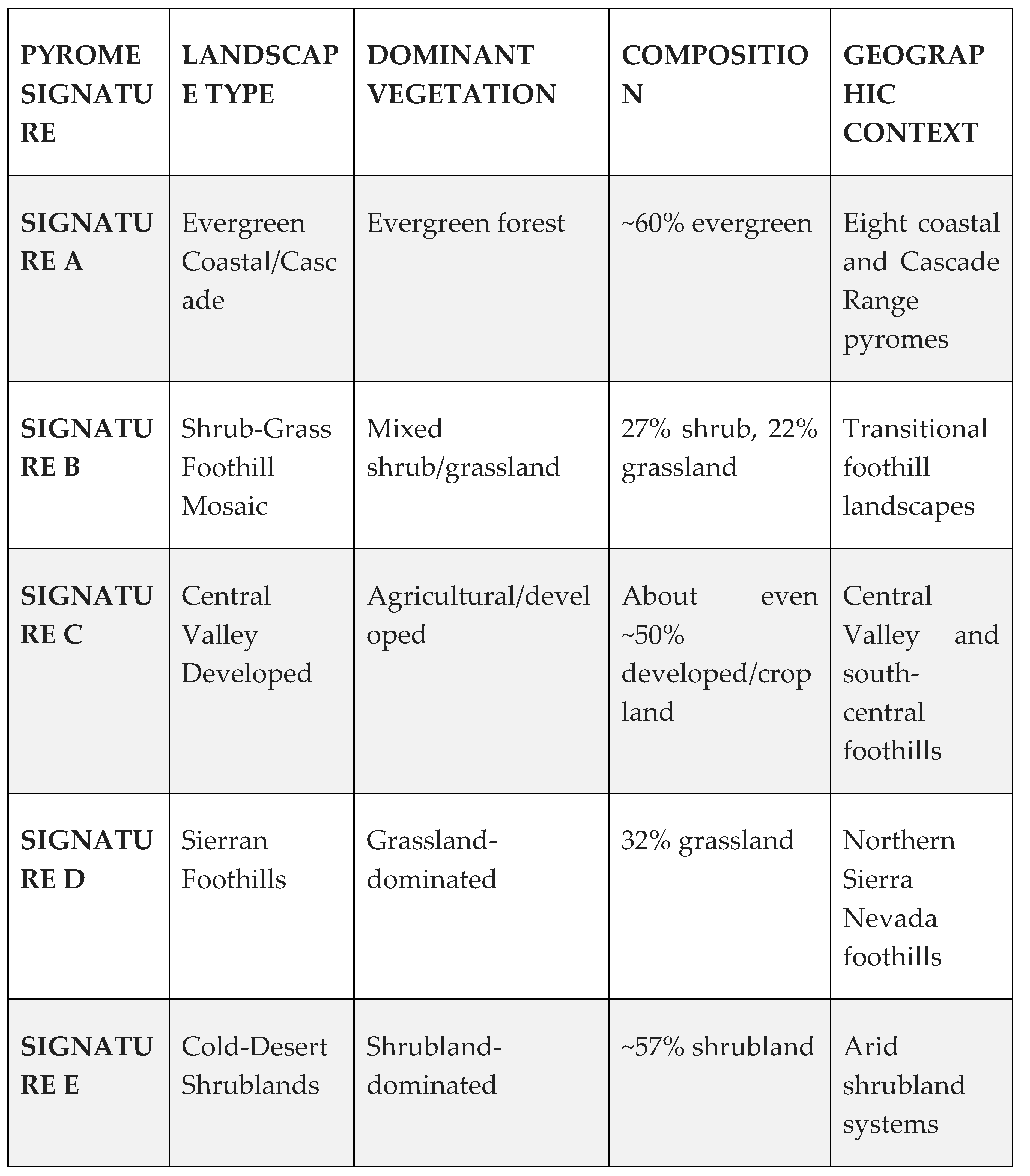
Table 3.
Pyrome characteristics of the final grouping of 19 initial pyromes. Grouping is based on the characteristic signature for each pyrome, which is based on the most common IV attributes for the variables shown in Table 1.
Table 3.
Pyrome characteristics of the final grouping of 19 initial pyromes. Grouping is based on the characteristic signature for each pyrome, which is based on the most common IV attributes for the variables shown in Table 1.
 |
2.4. Reconstructability Analysis Framework and Implementation
2.4.1. Fundamentals of Reconstructability Analysis
Reconstructability Analysis (RA) is introduced in this study to the wider GIS community as a technique for modeling categorical data that quantifies relationships between variables using information theory. While traditional statistical approaches often impose assumptions of linearity or normal distributions—assumptions frequently violated in environmental data—RA directly works with categorical variables (and/or continuous variables that have been discretized) to reveal structural patterns of dependency.
In the Variable-Based Reconstructability Analysis (VB-RA) approach employed in this study, models are represented as sets of relations between variables, where each relation captures a specific pattern of constraint in the data. These relationships are systematically organized in a lattice of structures, with the independence model at the bottom and the full data at the top. The Occam software (Zwick, 2004), developed at Portland State University, implements sophisticated algorithms to navigate this lattice efficiently, even for problems where this lattice is extremely large.
For those familiar with Bayesian Networks, RA shares the fundamental goal of using graph structures to model probabilistic relationships between categorical variables, but differs in several key aspects that make it particularly suitable for exploratory analysis (Zwick, 2004). While Bayesian Networks employ directed acyclic graphs (DAGs) to represent causal relationships and support probabilistic inference, RA uses undirected hypergraphs that can contain loops, allowing it to capture higher-order interactions among multiple variables simultaneously without requiring prior assumptions about causal direction (Zwick, 2004). This structural flexibility enables RA to discover unexpected high-ordinality and nonlinear interactions through systematic exploratory modeling, whereas Bayesian Networks typically require prior knowledge of causal structure and focus on confirmatory inference tasks. The hypergraph representation in RA can model some independence structures that are impossible in Bayesian Networks due to the acyclicity constraint, making RA particularly valuable for revealing complex interdependencies in systems where causal relationships are unknown or multidirectional (Harris and Zwick, 2021).
RA is rooted in Shannon’s Information Theory (Shannon, 1948) and Ashby’s Constraint Analysis (Ashby, 1956), with contributions from Klir, Krippendorff, and others who added graphical modeling approaches (Klir, 1985; Krippendorff, 1986). The methodology calculates the amount of information “transmitted” between discrete variables, resulting in a quantification of their relationships. For our wildfire research, we employ a directed system approach, where models are assessed by how much their independent variables (IVs) reduce the Shannon entropy (uncertainty) of a dependent variable (DV)—in our case, fire size classification (small or large).
The mathematical foundation is straightforward: Let p(DV) be the observed probability distribution of fire size; let pmodel(DV|IV) be the calculated model conditional probability distribution of fire size given the set of predicting IVs. Then:
and
H(DV) = −∑i p(DVi) log2 p(DVi)
Hmodel(DV|IV) = −∑ p(IVj) ∑i pmodel(DVi)|IVj) log2 pmodel(DVi)|IVj)
These two values represent the Shannon entropy (uncertainty) of fire size in the data (first equation) and the Shannon entropy of fire size in the RA model of the data (second equation). The latter entropy represents a reduction in the former entropy, with the difference between the original and reduced entropy serving as our information theoretic measure of predictive efficacy. Dividing this entropy reduction by H(DV) gives the fractional entropy reduction, expressed as a percentage, which is reported in Occam. This measure is specific to RA and other probabilistic machine learning methods. It is supplemented in Occam with generic metrics of predictive efficacy such as %Correct which are applicable to all machine learning methods.
2.4.2. Loop Versus Loopless Models in RA
Let Z be the DV, and A, B, C … be the IVs. A critical distinction in RA is between loopless models and models with loops. In our directed system with multiple independent variables (IVs) predicting a single dependent variable (fire size class), a loopless model contains only a single predicting component for the DV. For example, a loopless model like IV:ABCZ has only one predicting component (ABCZ), indicating that variables A, B, and C jointly predict Z. The “IV” component in this model is shorthand for ABC…. Every directed systems model includes a component that is a relation of all the independent variables (not only the predicting IVs). This is to assure that the directed systems models are hierarchically nested, which is desirable for statistical comparisons.
In contrast, a model with loops like IV:AZ:BZ:CZ has multiple predicting components (AZ, BZ, CZ) separated by colons, suggesting that variables A, B, and C quasi-independently contribute to Z prediction. (These IVs predict Z more independently than they do in IV:ABCZ, but the maximum entropy nature of RA methodology generates a kind of interaction effect among these IVs; see the discussion of different types of epistasis in (Zwick, 2011).) This model contains loops because every variable occurs in more than one relation. Loopless models offer computational advantages: they can be calculated algebraically without iterative procedures, and they represent a smaller model search space. Models with loops employ Iterative Proportional Fitting (IPF) which is substantially more computationally intensive, and thus better to run on a smaller subset of variables.
In our initial data exploration, we used loopless searches for feature selection, systematically evaluating all 45 original variables (dominant and subdominant vegetation classes across three rings and seven time periods, plus elevation, season, & ignition cause) to identify the most predictive features. This preliminary screening eliminated subdominant vegetation variables, which showed consistently low information content, allowing us to focus on dominant vegetation patterns in our subsequent analysis with models containing loops. This reduced the number of NLCD variables from 42 to 21, and also eliminated ignition cause.
2.4.3. Model Structure and Representation
In Reconstructability Analysis, models are hypergraphs whose components are relations between variables. These models form a structured lattice with the independence model (bottom), IV:DV, having the DV not related to any of the IVs, and the saturated model (top) having all variables related. This lattice provides a formalized model search space for identifying models that optimally balance parsimony with explanatory power.
For our analysis of multiple variables predicting fire size (Z), model notation follows the format:
IV:I0Z:M3Z:O6Z:SeasonZ:ElevZ
This model has five predictive components (relations), each involving one predicting IV, whose name is a string of letters that begins with a capital letter, and Z, the predicted DV. This notation indicates that the inner ring vegetation from T0 (I0), middle ring vegetation from T-15 (M3), outer ring vegetation from T- 30 (O6), month group (Monthgrp), and elevation (Elev) each independently predict fire size (Z). The first component (IV) represents all independent variables in their joint distribution, while each subsequent component following the colon represents a specific predictive relationship.
The search process navigates the lattice of structures from the independence model (IV:Z) through some number of increasingly complex levels, evaluating many models and retaining at each level some number of models specified in the configuration of the model run. This approach identifies the best models for a particular data set, and suggests models on which to run the Fit process which allows one to examine a particular model in full detail.
2.4.4. Search Strategy and Implementation
To identify optimal models within this vast lattice, we employ a bottom-up beam search strategy using the Occam3 software developed at Portland State University. This approach begins with the independence model (no predictive relationships) and systematically adds components that maximize information gain while maintaining statistical significance.
Our search configuration included:
- Search direction: Bottom-up
- Search width: 3 (number of models retained at each level)
- Search levels: 7 (maximum number of complexity levels explored)
- Search criteria to retain models at all levels: dBIC (delta Bayesian Information Criterion)
- Alpha threshold: 0.05 (statistical significance threshold)
This approach efficiently searches an extremely large space of possible directed models for the 23 IVs and one DV in our dataset without exhaustively enumerating all possible structures.
2.4.5. Model Evaluation Metrics
Models were evaluated using multiple information-theoretic criteria including:
- Information content, Inf: Proportion of system constraint captured, scaled from 0 (independence model) to 1 (data)
- Percent reduction in uncertainty, %dH(DV): Direct measure of how much the model reduces uncertainty about fire size, often the most useful metric. Because uncertainty has a logarithm in its mathematical expression even seemingly small values such as 8% can represent a large effect size such as a shift from 2:1 odds to 1:2 odds (Zwick, 2004).
- dBIC (ΔBIC): Bayesian Information Criterion difference (from a reference model), a conservative metric balancing accuracy and complexity
- dAIC (ΔAIC): Akaike Information Criterion difference (from a reference model), offering a less conservative alternative complexity-adjusted measure
- Classification accuracy: Percentage of correctly classified instances (small vs. large fires) (This is a general machine learning metric, not an information theoretic metric.)
While dBIC & dAIC measures were closely tracked, our primary criterion for model selection is a balance of %dH and %Cover, as these metrics tend to move in opposite directions. An increase in reduction of uncertainty is typically accompanied by reduction in the %Cover. The incremental alpha criterion picks the most complex model that is statically significant relative to the independence model reference and for which there’s a path from the reference to the model where every increment of complexity is also significant. All of the pyrome signature models that were evaluated using Fit for this study have a significant Incremental Alpha.
Table 2.
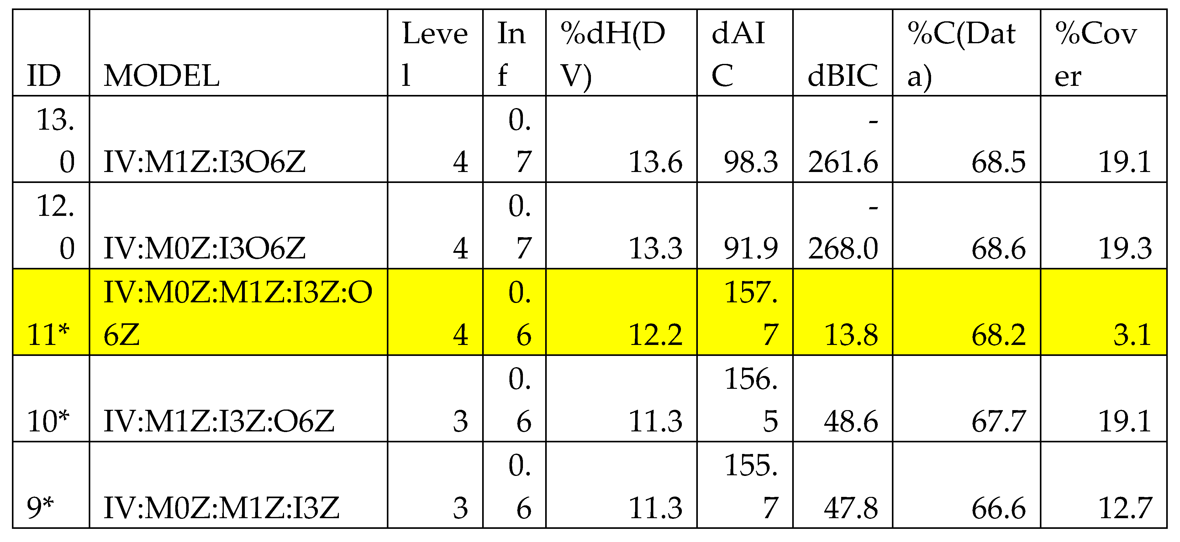
– Search output for pyrome signature B. A * in the ID column indicates a statistically significant model. Model structure is discussed in section 2.4.3. For this run, at each level only 3 models are retained, one extra relation is added per level. Metrics are discussed in section 2.4.5, and are in the next 4 columns. These are followed by %Correct, and finally %cover, the percent of the multivariate states of the predicting IVs that are actually present in the data.
Table 2.
– Search output for pyrome signature B. A * in the ID column indicates a statistically significant model. Model structure is discussed in section 2.4.3. For this run, at each level only 3 models are retained, one extra relation is added per level. Metrics are discussed in section 2.4.5, and are in the next 4 columns. These are followed by %Correct, and finally %cover, the percent of the multivariate states of the predicting IVs that are actually present in the data.
 |
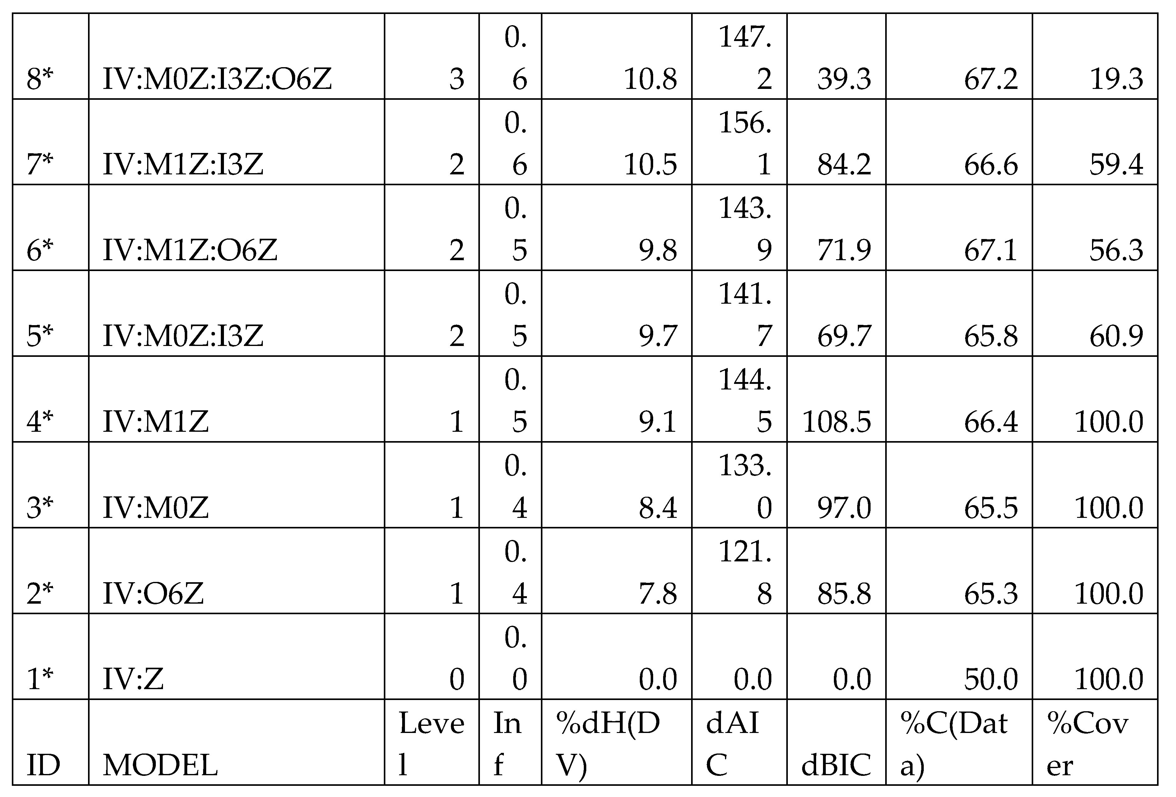 |
The output from a Search “run” is shown in Table 2, this is the actual output for signature group B (Mixed shrub–grass foothill mosaic). The highlighted row in the table indicates the model that was chosen for Fit processing. The %Cover, while low, is acceptable given the ecological constraints of the pyrome group. Not all NLCD classes will be present, for example evergreen forest would be rare or absent in a desert ecoregion.
2.4.6. Fit Analysis and Interpretation
After identifying candidate models through Occam’s Search function, we conducted detailed Fit analysis to examine exactly how vegetation patterns influence fire outcomes. The Occam Fit function calculated:
- Tables of conditional probabilities (given in %) of the two DV states given every combination of the states of the predictive IVs, classification rules for fire size prediction, and p-values for the statistical significance of the prediction rules (the probability of a Type 1 error in rejecting the hypothesis that the model conditional probabilities are the same as the DV margins of (50%, 50%).
- Performance metrics including sensitivity, specificity, and F1 score
- Tables of conditional DV probabilities, prediction rules, and p-values for each component relation
This detailed output enabled not just identification of which variables predict fire size, but specific understanding of the configurations most associated with large fire occurrence.
Table 3.
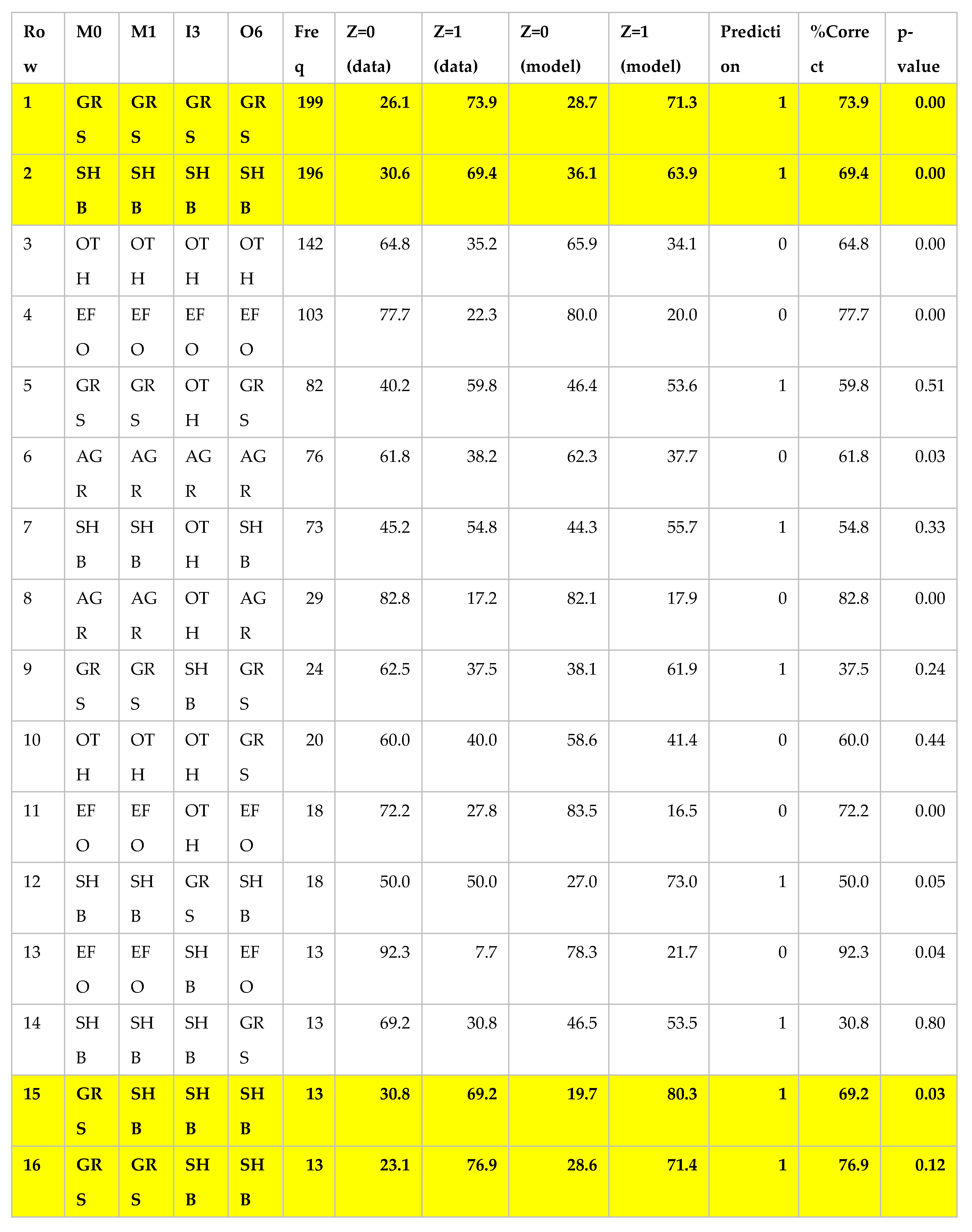
Example Fit output for model IV:M0Z:M1Z:I3Z:O6Z chosen as the best model by AIC and highlighted in Table 2. First four columns are the IVs in this model: Middle ring of layers 0 (T) and 1 (T-5), Inner ring of layer 4 (T-20), and Outer ring of layer 6 (T-30). Table is sorted on frequency. The next four columns are the conditional probability distribution, p(Z|IV) of the data for this each IV state, and the model’s predicted conditional distribution, pmodel(Z|IV). The prediction column states the Z value predicted by this model for this particular IV state. %Correct is the accuracy of the model prediction for this IV state, p-value is reported last. GRS is Grassland, SHB is Shrub/Scrub, EFO is Evergreen Forest, AGR is Cultivated Crops, & OTH is our bin for the “non-vegetated” classes). Yellow bold draws attention to the rows with high probability of large fire predicted by this model for this configuration of NLCD values.
Table 3.
Example Fit output for model IV:M0Z:M1Z:I3Z:O6Z chosen as the best model by AIC and highlighted in Table 2. First four columns are the IVs in this model: Middle ring of layers 0 (T) and 1 (T-5), Inner ring of layer 4 (T-20), and Outer ring of layer 6 (T-30). Table is sorted on frequency. The next four columns are the conditional probability distribution, p(Z|IV) of the data for this each IV state, and the model’s predicted conditional distribution, pmodel(Z|IV). The prediction column states the Z value predicted by this model for this particular IV state. %Correct is the accuracy of the model prediction for this IV state, p-value is reported last. GRS is Grassland, SHB is Shrub/Scrub, EFO is Evergreen Forest, AGR is Cultivated Crops, & OTH is our bin for the “non-vegetated” classes). Yellow bold draws attention to the rows with high probability of large fire predicted by this model for this configuration of NLCD values.
 |
 |
The Fit output is quite voluminous when the model is complex. Table 3 shows a medium complexity example with four IVs each having 8 possible states. This is the model chosen from Table 3 as the best representative for signature group B, and in its entirety shows every possible combination in this data set (126 rows for these data). Here we show just the top section of the table, sorted in reverse order by frequency of occurrence of this specific combination of IV states in this data set. The data columns (Z=0 & Z=1) are showing the distribution of 1’s and 0’s in this data set, for this each combination of IV values. Note that when the model is correct, the % correct is the probability of the predicted state (either Z=0 or Z-=1) in the data itself. The model is correct for all IV states (rows) except for rows 9 and 14. In this table the p-values vary widely, but in the rows that are most important (high frequency, and correct prediction) they are significant. (In the two rows where the prediction is incorrect, the p-values are very far from significant.) In this table we see combinations of all GRS (Grassland) are the highest frequency combination, and also nearly the most fire-prone (71.3%), only exceeded by rows 15 & 17 which are mixtures of shrubs & grasses. Row 2 is all Shrub/Scrub and has a high probability of large fires according to the data and our model. This model includes layer 6 (06), which is from 30 years prior, as a significant predictor of the DV. If we wanted to drill down and see the direct effect of IV O6 on the model, there are sub-tables that show the direct contribution of each element of the model.
Table 4.
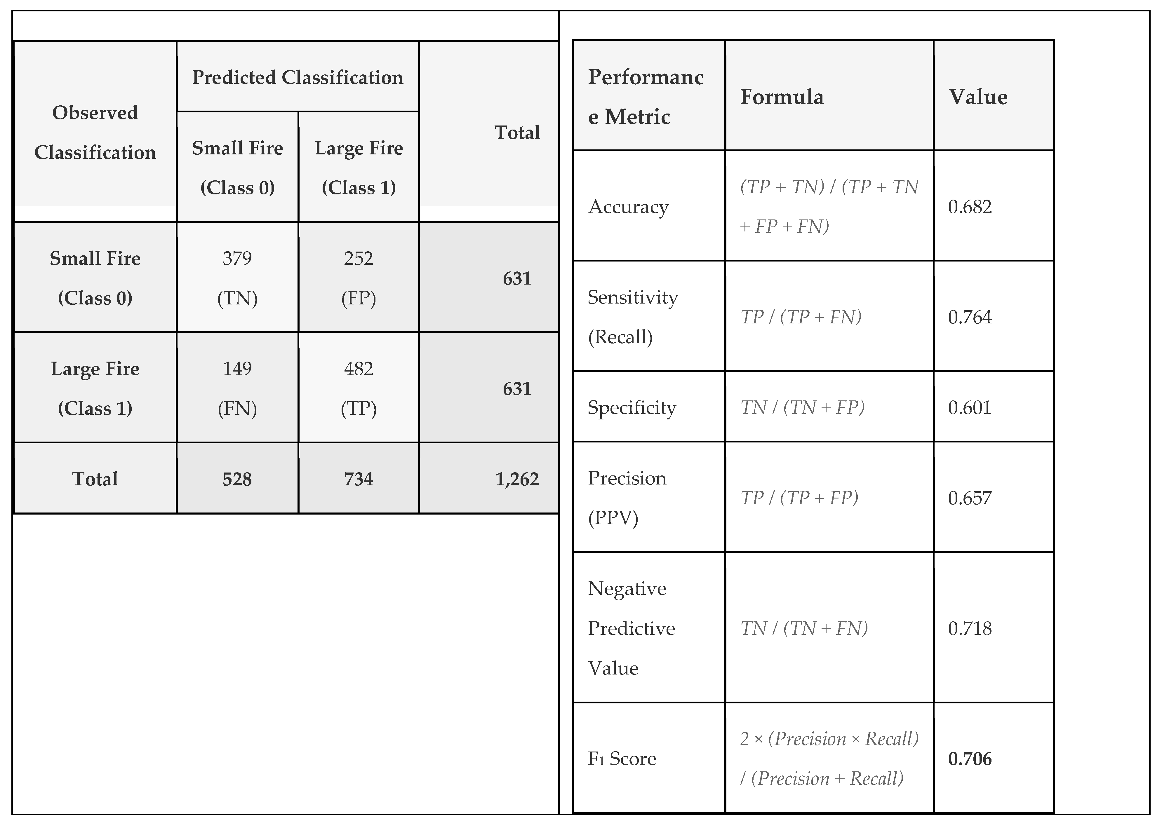
A & B – A (left) Confusion matrix for pyrome Signature B model IV:M0Z:M1Z:I3Z:O6Z. TN is True Negative, FN is False Negative, FP is False Positive, & TP is True Positive. The marginals are the total row and column counts. B (right) performance metrics for this model.
Table 4.
A & B – A (left) Confusion matrix for pyrome Signature B model IV:M0Z:M1Z:I3Z:O6Z. TN is True Negative, FN is False Negative, FP is False Positive, & TP is True Positive. The marginals are the total row and column counts. B (right) performance metrics for this model.
 |
2.4.7. Validation Approach
We implemented a rigorous validation strategy to ensure model reliability. This included a holdout approach with 20% of wildfire data reserved for testing. The %Correct on the test and train data corresponded well enough to confirm that the models were robust, so final Fit models were run on the entire pyrome data set without holding out any test data.
Additionally, we performed five-fold cross-validation using different random seeds (11, 22, 33, 42, 55) for sampling the small fires, which greatly outnumber large fires in the natural distribution (Figure 6). Results remained consistent across all sampling seeds, confirming the robustness of our findings, with the final analysis using seed 55.
3. Results
3.1. Multi-Scale Predictive Patterns Across Temporal Scales
Reconstructability analysis of wildfire behavior across five distinct pyrome signatures reveals fundamental differences in how landscape patterns at multiple temporal scales influence fire size outcomes. Each pyrome exhibits unique temporal-spatial “memory” signatures that reflect their underlying ecological characteristics and fire behavior patterns, and grouping them by signature leads to classification accuracies of 69.1% to 73.2% and uncertainty reduction ranging from 6.1% to 18.0% depending on landscape characteristics. Recall that it was noted earlier that an uncertainty reduction as low as 8% can represent a large effect size.
Each pyrome signature group has a distinct pattern of model that Occam produced, except that C & D have identical structures (different Fit results, however). We see that older vegetation is statistically significant in most of the models. Throughout all model configurations, grassland and shrubland dominance were consistently associated with higher probabilities of large fires, while areas dominated by evergreen forest or developed land showed lower probabilities for this outcome. The outer rings proved to be quite predictive in many of the models, as we will see in the detailed sections that follow.
3.2. Analysis of Occam Search and Fit Results by Pyrome
The primary groupings within the data set are the pyrome signature groups (Figure 7), the construction of which is discussed in the Methods section. Here we take the five final groupings and summarize the results of our extensive analysis of the Search and Fit results for each. The model structures all have the DV in the relation, so a model element will read M3Z, meaning that the Middle ring of layer 4 (T- 20) has an influence on the fire size target variable. Figure 8 summarizes the temporal and spatial components of all five pyrome models.
Evergreen Coastal (Signature A) achieved 69.1% classification accuracy with 6.1% uncertainty reduction using the three-variable model IV:M0Z:I3Z:ElevZ. This model incorporates current middle ring conditions (M0Z), inner ring patterns from T-15 (I3Z), and elevation (ElevZ). Signature A was the only pyrome where elevation emerged as a significant predictor. This pyrome signature produced the worst %dH of any of our modeling.
Shrub-Grass Foothill Mosaic (Signature B) achieved 70.0% accuracy and 11.7% uncertainty reduction using the four-variable model IV:M0Z:M1Z:I3Z:O6Z. This model incorporates current middle ring conditions (M0Z), middle ring patterns from T-5 (M1Z), inner ring patterns from T-15 (I3Z), and outer ring patterns from T-30 (O6Z). This signature covers a large portion of our study area, and has highly predictive results.
Central Valley Developed/Agricultural (Signature C) achieved the highest predictive performance with 73.2% classification accuracy and 18.0% uncertainty reduction using model IV:I0Z:O1Z:O6Z. This three-variable model incorporates current inner ring conditions (I0Z), outer ring patterns from T-5 (O1Z), and outer ring patterns from T-30 (O6Z). This very small part of our study area has the best results.
Northern Sierran Foothills (Signature D) employed an identical model structure to Signature C (IV:I0Z:O1Z:O6Z) achieving 69.2% accuracy and 8.4% uncertainty reduction. The model incorporates current inner ring conditions (I0Z), outer ring patterns from T-5 (O1Z), and outer ring patterns from T-30 (O6Z). This small portion of the study area also had quite good results.
Desert Shrublands (Signature E) achieved 70.3% accuracy and 8.0% uncertainty reduction using the four-variable model IV:I0Z:O0Z:O1Z:O3Z. This model incorporates current inner ring conditions (I0Z), current outer ring conditions (O0Z), outer ring patterns from T-5 (O1Z), and outer ring patterns from T-15 (O3Z). This is the largest signature group by area and has predictive and useful results.
Cross-Pyrome Temporal Patterns
Analysis across all pyromes revealed systematic patterns in temporal-spatial variable usage:
Immediate Risk Indicators (T-0): Inner ring dominance (I0Z) was significant in Signatures C, D, and E. Middle ring patterns (M0Z) were significant in Signatures A and B. Current outer ring conditions (O0Z) were significant only in Signature E.
Historical Memory Effects: T-30 outer ring patterns (O6Z) were significant in Signatures B, C, and D. T-15 inner ring patterns (I3Z) were significant only in Signatures A and B. T-5 middle ring patterns (M1Z) were significant only in Signature B.
Temporal Complexity: Models ranged from three-variable structures (Signatures A, C, D) to four-variable structures (Signatures B, E), all including multiple time variables.
Vegetation Risk Assessment
Grassland ignitions consistently showed 75-85% large fire probability across all pyromes. Desert shrubland persistence patterns showed 68-70% risk, while shrub-grass mosaics ranged from 69-77% risk. Developed/agricultural areas showed 21-36% large fire probability, dense evergreen forest showed 43-55% risk, and evergreen patches within shrub-dominated landscapes showed 22% large fire probability. Figure 9 summarizes the vegetation across all five pyromes.
4. Discussion
4.1. Multi-Scale Vegetation Patterns as Predictors of Fire Size
Old Vegetation Plays a Role
When we built this model using 30 years of NLCD data, we could have easily not seen a signal from the old vegetation layers. We could have found models that only produced significance from the most current layers of data. The fact that we see a strong signal from old vegetation, in specific pyromes, makes this a strong argument for using these data for wildfire planning. While we see in pyrome signature A that there is just a signal coming from more recent layers (T-15), in signatures B, C, & D the T-30 outer ring is a strong predictor. All of the models use at least one layer that is 15 years or older. Ignition cause does not significantly discriminate between large and small fires, so it was dropped from subsequent analysis. Time of year (season) was also not particularly useful, since most of the fires occur in the Summer, so this variable was dropped during further analysis. Elevation was only significant in the Evergreen dominated signature A.
Interpretation of Pyrome-Specific Patterns
The distinct temporal-spatial modeling requirements of each pyrome reflect fundamental differences in landscape fire behavior.
- Signature A’s (IV:M0Z:I3Z:ElevZ) elevation dependency perhaps reflects the importance of topographic moisture gradients in evergreen-dominated landscapes, while its lower uncertainty reduction reflects that we are likely missing important variables. Pyrome signature A’s results are poor enough that we could easily state that we have nothing useful to say about this signature. Since this pyrome has an extensive footprint in the study area this is unfortunate.
- Signature B’s (IV:M0Z:M1Z:I3Z:O6Z) temporal complexity reflects perhaps the interplay between grasses and shrubs, requiring a multi-temporal model to capture fire behavior patterns. The four-variable model spanning T-0 to T-30 suggests when these landscapes lead to large fires it is often due to older vegetation. In this pyrome, evergreen forests appear to be protective against large fires.
- Signature C’s (IV:I0Z:O1Z:O6Z) exceptional performance reflects the stark contrasts between extreme grassland fire risk (85% large fire probability) and moderate developed areas (23-36% risk), creating clear predictive patterns in this human-modified landscape. The reliance on both immediate and historical conditions is consistent with the other pyromes, in this smallest of the signature groups.
- Signature D’s (IV:I0Z:O1Z:O6Z) structural similarity to Signature C but lower uncertainty reduction suggests more heterogeneous fire behavior patterns in this grassland-dominated landscape. The grasses and shrubs in this ecoregion have high risk in our model with 79%, and 67%, respectively. While this pyrome is the smallest of our groupings, it has a unique fire behavior. This pyrome group contrasts with signature B, evergreen forests here have a moderate risk (52%) of large fires. Grasses and shrubs have high large fire risk, similar to all of the other pyromes.
- Signature E’s (IV:I0Z:O0Z:O1Z:O3Z) unique multi-temporal outer ring model suggests fire behavior depends heavily on a broad spread of shrubs maintained across a shorter period of time (T-15), rather than the T-30 patterns important in some other pyromes. The patterns of shrub and grassland leading to large fires is prevalent, while the damping effect of evergreen forests is similar to signature B.
Cross-Pyrome Temporal Pattern Interpretation
The systematic patterns in temporal-spatial variable usage likely reveal fundamental ecological processes. Immediate Risk Indicators (T-0) show that inner ring dominance is critical for immediate fire behavior in human-modified landscapes (Signatures C, D, E), while middle ring patterns are more important in evergreen and mixed systems (Signatures A, B). Current outer ring conditions are significant only in desert shrublands, perhaps reflecting slow growth of this vegetation in these conditions.
Historical memory effects demonstrate that most landscapes retain 30-year structural memory that influences contemporary fire behavior, as evidenced by the widespread importance of T-30 outer ring patterns. However, T-15 inner ring patterns are significant only in forested landscapes (A, B), indicating development cycles specific to these systems.
Vegetation Risk Pattern Interpretation
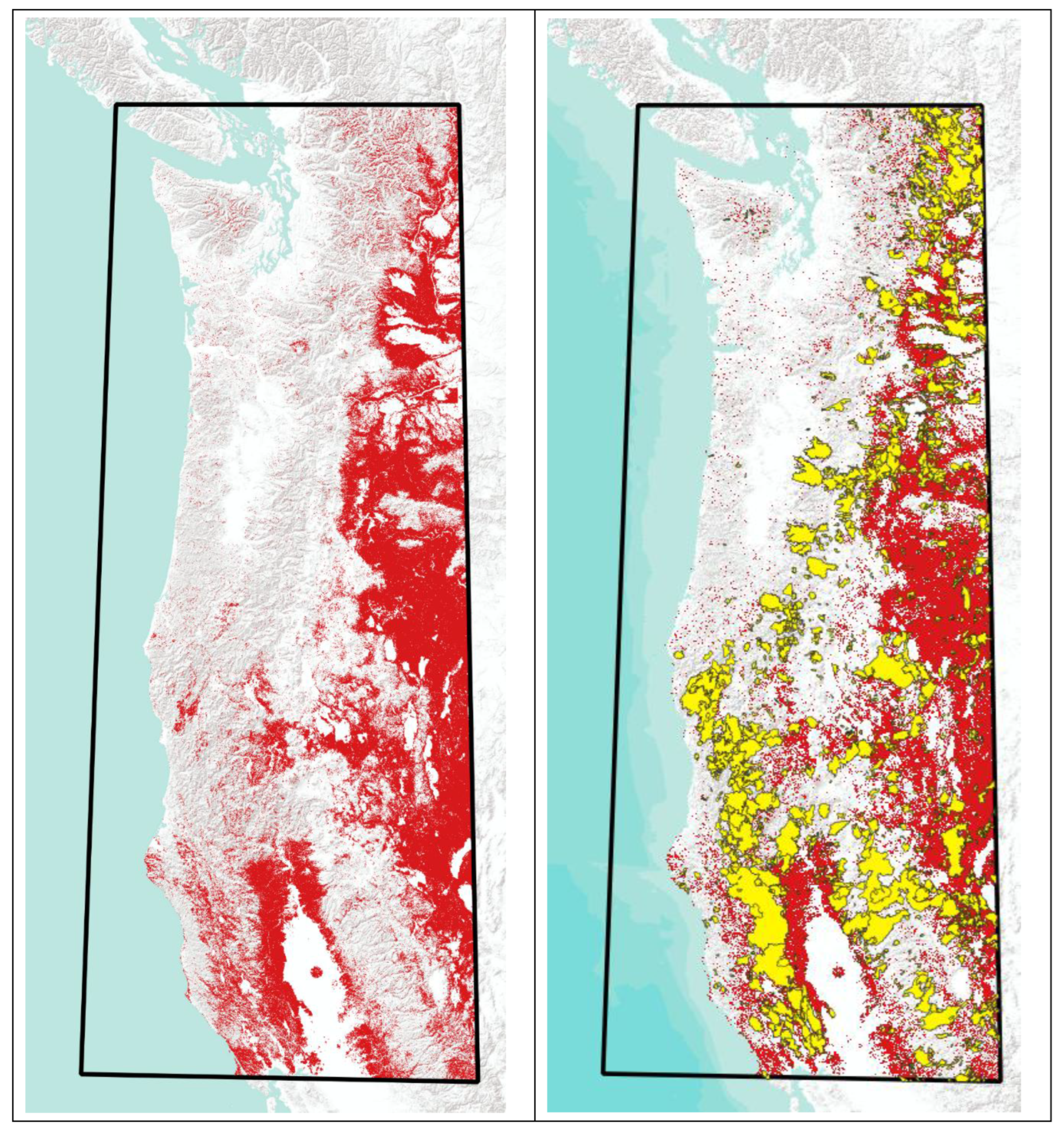
The quantified vegetation risk patterns confirm and extend established understanding of fuel-fire relationships. The consistently high risk associated with grassland ignitions (75-85%) reflects the rapid flame spread characteristics and low moisture content of herbaceous fuels. The moderate risk in developed/agricultural areas (21-36%) demonstrates their function as effective fuel breaks, while the protective effect of dense evergreen forest (43-55%) reflects moisture retention capacity and reduced flame spread rates. The particularly strong protective effect of evergreen patches within shrub-dominated landscapes (22%) suggests that under certain conditions trees act as a fire buffer. For most of the study area long-term established grasses and shrubs indicate an enhanced risk of large fires. To assess the impact of this finding, Figure 10 shows a spatial query of the NLCD layers where the 1985 shrubs and grasses are also present in the same cells in 2020. No queries were done to determine if anything occurred during that 35-year interval. The second graphic shows the same data overlaid with the fire perimeter data for the same time period, extended to 2024. There are clearly large areas where shrubs and grasses have persisted that have not burned yet, but are likely to have large fires, if they ignite. We also attempted an overlay of wind speed, but the results were limited, and require more investigation.
Methodological Contributions
This study demonstrates several methodological advances in wildfire risk assessment:
Multi-scale Temporal Analysis: The systematic evaluation of vegetation patterns across T-0 to T-30 time periods revealed that different landscape types have fundamentally different temporal memory requirements, resulting in differing recommendations for mitigation of large fires through local planning and intervention.
Information-Theoretic Quantification: Reconstructability analysis provides transparent, interpretable models with explicit uncertainty reduction measures. The range from 6.1% to 18.0% uncertainty reduction represents substantial predictive improvements over baseline conditions, with practical implications for fire management decision-making.
Pyrome-Specific Modeling: Rather than assuming uniform fire behavior patterns across landscape types, our approach identified distinct “temporal memory signatures” for each pyrome, with performance optimization requiring landscape-specific variable combinations. Different pyrome clustering approaches yield varied results, which could be useful in further studies.
Categorical Data Integration: The dominance-based ring buffer approach successfully converted complex spatial patterns into categorical predictors suitable for Reconstructability Analysis, avoiding the limitations of variable transformations like one-hot encoding, while retaining ecological interpretability.
4.5. Methodological Contributions of Geospatial RA
This study demonstrates a novel integration of multi-scale GIS analysis with information-theoretic modeling that extends both fields. The dominance-based concentric ring buffer approach represents a significant advancement over conventional point-based or uniform buffer analyses common in wildfire studies. By extracting dominant and subdominant vegetation classes at three distinct spatial scales, we developed categorical predictors that retain high interpretability while avoiding the sparsity issues that plague many categorical data analyses. This GIS methodology could be readily adapted to other point-based environmental phenomena where surrounding landscape context is theoretically important.
The application of Variable-Based Reconstructability Analysis to this geospatial dataset showcases the unique capabilities of information-theoretic modeling for categorical spatial data. Unlike traditional statistical models that impose linearity assumptions or machine learning approaches that sacrifice interpretability, RA provides:
- Structural transparency: The model notation (e.g., M0Z:M1Z:I3Z:O6Z ) directly expresses the detected relationships between variables, making the models immediately interpretable to domain experts (Klir, 1985; Zwick, 2004).
- Optimal model selection: The information-theoretic criteria (dBIC, dAIC) provide rigorous mathematical tools for navigating the trade-off between model complexity and fidelity to the data (Burnham and Anderson, 2002).
- Multi-scale integration: By systematically exploring combinations of predictors from different spatial and temporal scales, RA effectively identifies cross-scale interactions that might be difficult to detect with conventional methods.
- Categorical data efficiency: RA naturally accommodates nominal data without requiring dummy variables or other transformations that can inflate dimensionality and degrade model performance.
The entire analytical pipeline—from the custom GIS extraction functions to the Occam-based RA modeling—exemplifies how spatial data science can bridge the gap between theoretical understanding and practical prediction. This approach offers particular promise for complex spatial systems where predictive variables are often categorical, spatial dependencies span multiple scales, and interpretability is crucial for operational implementation.
Research has established that non-forest lands have more area burned, increased fire cycles, and larger fire sizes than forested areas (Crist, 2023). Our contribution is not in discovering these relationships, but rather in applying a novel information-theoretic methodology that quantifies their relative importance and interactions across spatial and temporal scales, providing a complementary approach to extend existing fire behavior models.
5. Methodological Comparison
To contextualize our Reconstructability Analysis approach within the broader landscape of fire prediction modeling, we conducted a comparative assessment against alternative methodologies. This comparison helps illuminate the relative strengths and limitations of the RA approach for categorical spatial data analysis.
5.1. Comparison with other Machine Learning approaches
Contemporary wildfire prediction often employs machine learning techniques such as random forests, support vector machines, and neural networks (Jain et al., 2020; Nadeem et al., 2020). While these approaches can achieve high predictive accuracy, they typically function as “black box” models, obscuring the specific variable interactions driving predictions (Molnar, 2020). This opacity can limit their utility in operational contexts where decision justification and interpretability are essential for management applications (Coffield et al., 2019).
As outlined in Section 4.5, RA’s structural transparency and categorical data efficiency contrast sharply with these limitations. For example, the model for signature group B, M0Z:M1Z:I3Z:O6Z, explicitly indicates that the inner ring vegetation from T-20, along with middle ring vegetation from T-0 & T-5, and outer ring vegetation from T-30 quasi-independently influence fire size classification. The model is broken down in the Fit output so that the predictions of individual IVs, such as the Outer Ring at 30 years lag, and predictions of the states of multiple IVs can be examined in detail.
Machine learning approaches also frequently struggle with categorical variables, often requiring one-hot encoding that exponentially increases dimensionality or ordinal encoding that imposes an artificial ordering on nominal categories. In contrast, RA naturally accommodates categorical data without transformation, preserving the fundamental categorical nature of vegetation classifications.
5.2. Comparison with Traditional Statistical Methods
Traditional statistical approaches for categorical data analysis include logistic regression, log-linear models, and chi-square tests. While these methods offer statistical rigor and established inference procedures, they face limitations when modeling complex multivariate relationships in spatial data.
Logistic regression, often used for binary outcomes like our fire size classification, requires assumptions about linearity in the logit scale and typically struggles with high-dimensional categorical predictors. The 42 categorical variables in our analysis would require extensive dummy coding and interaction terms, making model selection and interpretation challenging.
RA effectively functions as an automated, information-theoretic approach to log-linear modeling, with the advantage of systematic model search and selection procedures. Rather than manually specifying and testing interactions, RA algorithmically identifies the most informative variable relationships within the lattice of possible models.
Additionally, traditional statistical approaches often focus on hypothesis testing rather than prediction. Our RA methodology bridges this gap, providing both theoretical model fit metrics (%ΔH, ΔBIC) and practical predictive performance measures (%Correct). Occam can be used for both exploratory and confirmatory modeling.
6. Conclusions
This study demonstrates that simple, interpretable variables extracted from vegetation structure and topography surrounding ignition points can significantly aid in predicting wildfire size outcomes. Dominant vegetation within the immediate vicinity of an ignition site, particularly shrublands and grasslands, emerged as consistent predictors of fire escalation. Furthermore, the historical persistence of these vegetation types, as revealed through the temporal ring buffer analysis, added additional explanatory power, underscoring the importance of landscape history in influencing fire behavior.
Using RA model structures with loops revealed complex interactions between spatial and temporal variables, particularly the synergy between outer-ring and inner-ring vegetation patterns. These findings suggest that the risk of a small ignition growing into a large wildfire is due to current conditions that reflect the consequences of historical vegetation dynamics over a broader spatial context.
Importantly, the use of Variable-Based Reconstructability Analysis (VB-RA) provided a transparent and readily interpretable alternative to black-box machine learning models. By emphasizing parsimony and interpretability, VB-RA enables us to identify minimal yet powerful combinations of predictors without overfitting, aligning with practical needs for real-world wildfire management.
The results obtained in this study are likely dependent on the grouping and binning that were applied to the data. Different vegetation bins would certainly produce different results, and clearly different pyrome groupings will affect the output. A different sampling approach to the three-ring buffer sizes would produce different inputs, and a different temporal sampling strategy would also have an effect. Despite these underlying choices, we feel confident that the results obtained do reflect what is actually affecting the size of wildfires. Figure 10 shows in red the areas that are predicted to be susceptible to large wildfires.
Future work should expand this analysis by integrating climatic variables, soil moisture indices, and finer-grained topographic derivatives such as aspect and ruggedness. Wind modeling will play an important role in operationalizing the results from our study, particularly in the grasses and shrub dominated areas. Better granularity in the vegetation layer would be useful. Lastly, linking ignition causes to eventual burn severity could offer a more comprehensive understanding of wildfire impacts beyond simple size classifications.
Overall, this study quantifies the well-established relationships between vegetation patterns and wildfire behavior using information-theoretic methods. While fire scientists and managers may already recognize the importance of these factors (Stephens et al., 2014; Westerling, 2016), our approach offers a transparent and interpretable framework for measuring their relative contributions to fire risk. Especially with regard to the age of the vegetation. Research has established that non-forest lands have more area burned, increased fire cycles, and larger fire sizes than forested areas (Crist, 2023). Our contribution is not in discovering these relationships, but rather in applying a novel information-theoretic methodology that quantifies their relative importance and interactions across spatial and temporal scales, providing a complementary perspective to existing fire behavior models.
References
- Abatzoglou, J.T. and Williams, A.P. (2016) ‘Impact of anthropogenic climate change on wildfire across western US forests’, Proceedings of the National Academy of Sciences, 113(42), pp. 11770–11775.
- Ashby, W.R. (1956) An introduction to cybernetics. Chapman & Hall.
- Balch, J.K. et al. (2013) ‘Introduced annual grass increases regional fire activity across the arid western USA (1980–2009’, Global Change Biology, 19(1), pp. 173–183.
- Bradley, B.A. et al. (2018) ‘Disentangling the abundance–impact relationship for invasive species’, Proceedings of the National Academy of Sciences, 116(20), pp. 9919–9924.
- Burnham, K.P. and Anderson, D.R. (2002) Model selection and multimodel inference: A practical information-theoretic approach. 2nd edn. Springer.
- Coffield, S.R. et al. (2019) ‘Machine learning to predict final fire size at the time of ignition’, International Journal of Wildland Fire, 28(11), pp. 861–873.
- Crist, M.R. (2023) ‘Rethinking the focus on forest fires in federal wildland fire management: Landscape patterns and trends of non-forest and forest burned area’, Journal of Environmental Management, 327, p. 116718. Available at: . [CrossRef]
- Dillon, G.K. et al. (2011) ‘Both topography and climate affected forest and woodland burn severity in two regions of the western US, 1984 to 2006’, Ecosphere, 2(12), pp. 1–33.
- Finney, M.A. et al. (2005) ‘On the need for a theory of wildland fire spread’, International Journal of Wildland Fire, 14(4), pp. 347–356.
- Jain, P. et al. (2020) ‘A review of machine learning applications in wildfire science and management’, Environmental Reviews, 28(4), pp. 478–505.
- Klir, G.J. (1985) Architecture of systems problem solving. Plenum Press.
- Krippendorff, K. (1986) Information theory: Structural models for qualitative data. Sage Publications.
- Molnar, C. (2020) Interpretable machine learning: A guide for making black box models explainable. Lulu Press.
- Nadeem, K. et al. (2020) ‘Mesoscale spatiotemporal predictive models of daily human-and lightning-caused wildland fire occurrence in British Columbia’, International Journal of Wildland Fire, 29(1), pp. 11–27.
- NWCG (2020) Glossary of wildland fire terminology. NWCG.
- Percy, D. and Zwick, M. (2024) ‘Information-Theoretic Modeling of Categorical Spatiotemporal GIS Data’, Entropy, 26(9), p. 784.
- Shannon, C.E. (1948) ‘A mathematical theory of communication’, The Bell System Technical Journal, 27(3), pp. 379–423.
- Stephens, S.L. et al. (2014) ‘Managing forests and fire in changing climates’, Science, 342(6154), pp. 41–42.
- Westerling, A.L. (2016) ‘Increasing western US forest wildfire activity: sensitivity to changes in the timing of spring’, Philosophical Transactions of the Royal Society B: Biological Sciences, 371(1696), p. 20150178.
- Zwick, M. (2004) ‘An overview of reconstructability analysis’, Kybernetes, 33(5/6), pp. 877–905.
Figure 1.
Location of study, located on the West coast of the USA between the Canadian border and just North of San Francisco, extending inland to acquire a variety of vegetation patterns. Colors represent land classification from National Land Cover Database (NLCD) as shown in Figure 2.
Figure 1.
Location of study, located on the West coast of the USA between the Canadian border and just North of San Francisco, extending inland to acquire a variety of vegetation patterns. Colors represent land classification from National Land Cover Database (NLCD) as shown in Figure 2.
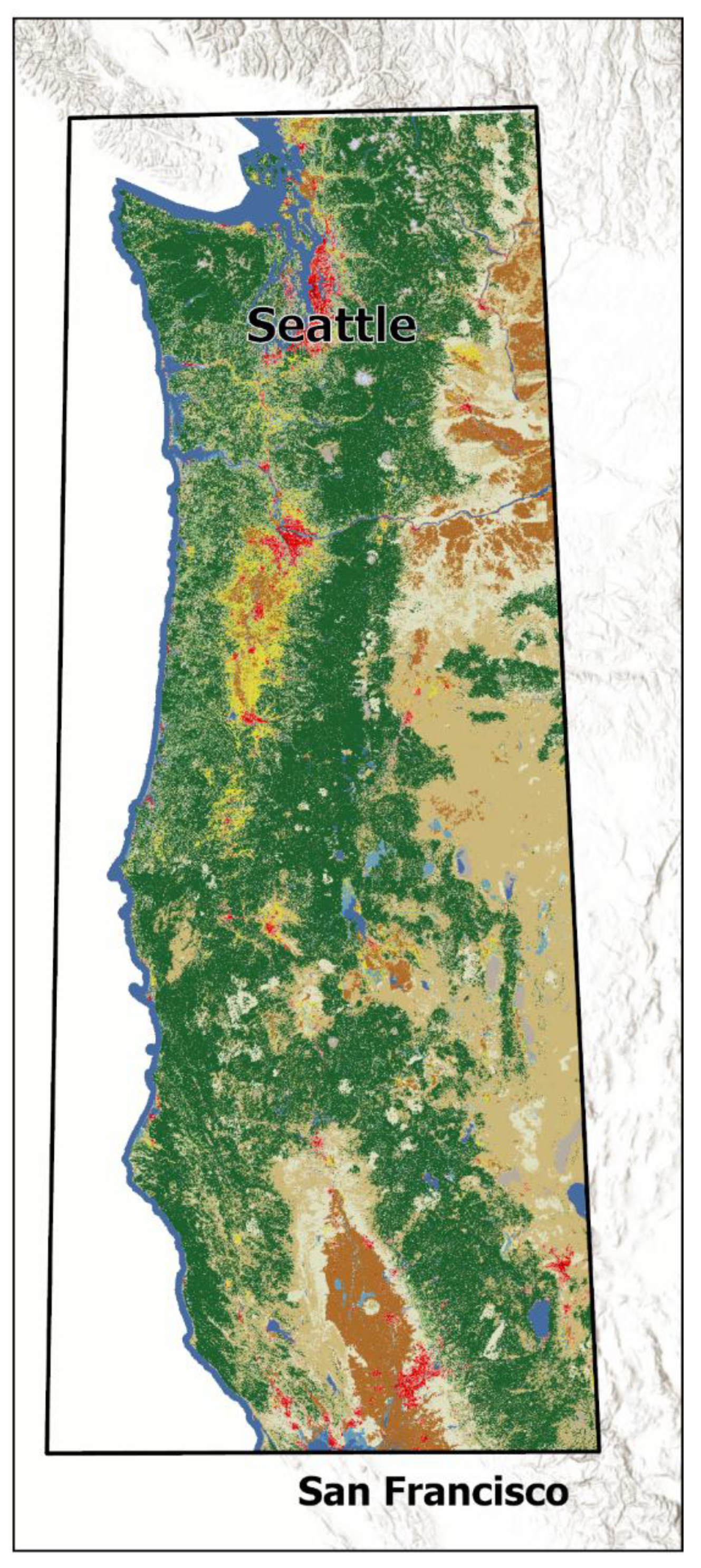
Figure 8.
Cross Pyrome variable comparison. Times with no variables are not included, so T-10, T-20, and T-25 are missing. Elevation was only significant in Pyrome A, dominated by forests. Immediate conditions (I0) are not significant in Pyromes A & B, while relying on the middle ring for a signal. The oldest and farthest ring, O6 is significant in Pyromes B, C, & D. Reduction of uncertainty is the %dH column, Evergreen dominated signature A is our worst result with only 6.1 % reduction. The other pyrome models perform much better, with the best results from C (18% reduction of uncertainty).
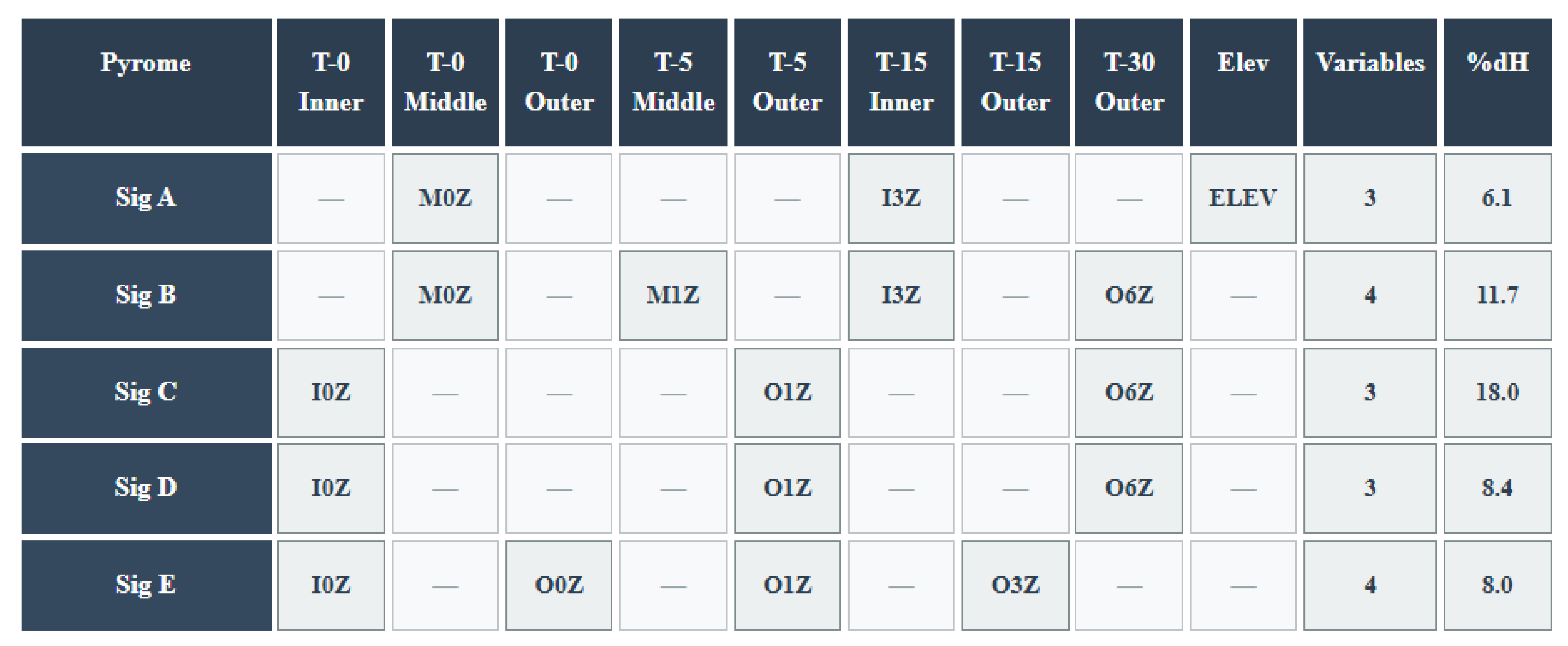
Figure 9.
Grid showing each pyrome with its vegetation patterns and relative risk for large fire. These are summarized from the individual Fit tables from Occam.
Figure 9.
Grid showing each pyrome with its vegetation patterns and relative risk for large fire. These are summarized from the individual Fit tables from Occam.
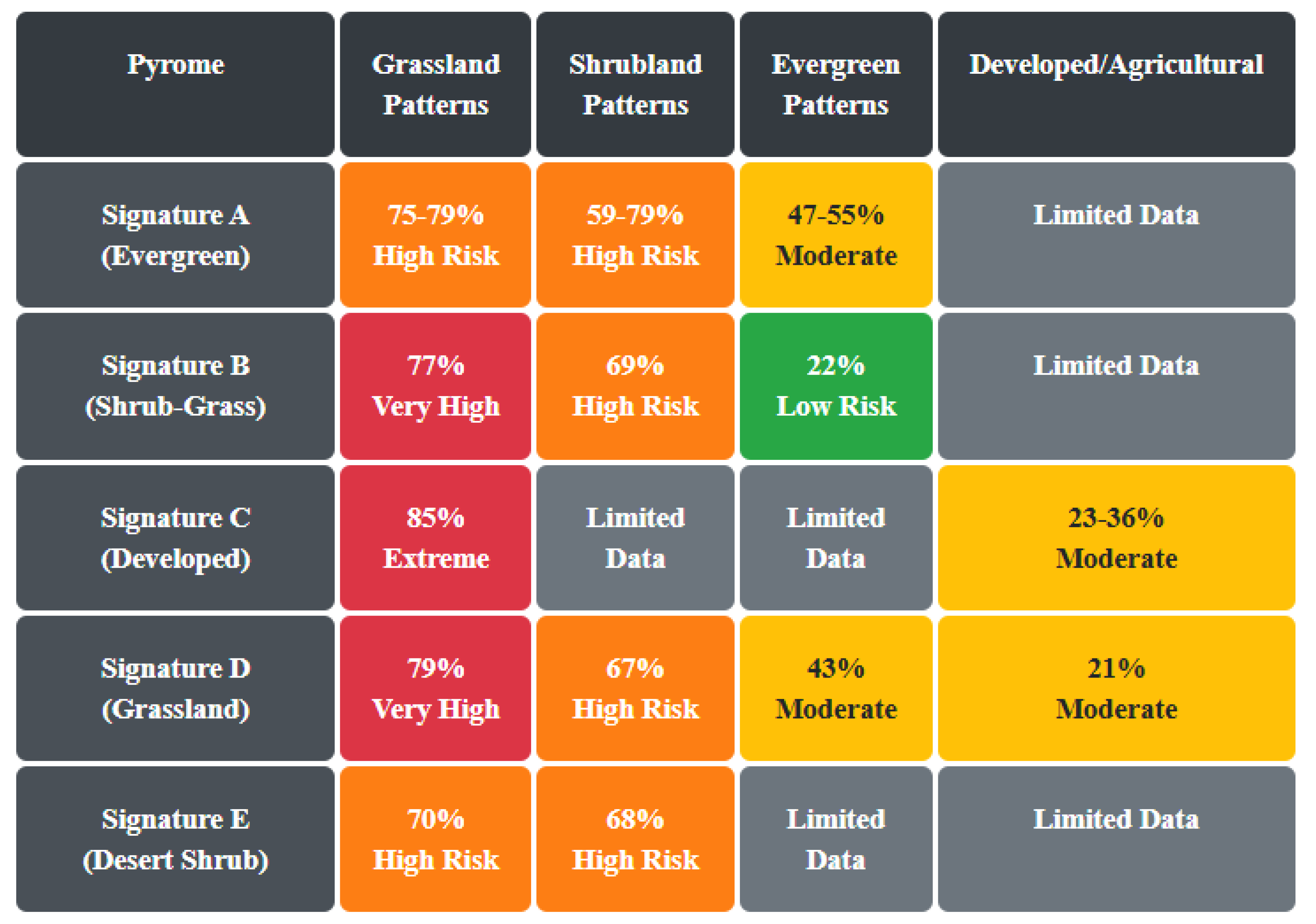
Figure 10.
Persistent shrubs and grasses. Study area locations where (left) red indicates Grassland or Shrub/Scrub have persisted from 1985 to 2020, indicating a higher probability of large fires, based on our model. On the right is an overlay of the burn perimeters in yellow from 1985 to 2024.
Figure 10.
Persistent shrubs and grasses. Study area locations where (left) red indicates Grassland or Shrub/Scrub have persisted from 1985 to 2020, indicating a higher probability of large fires, based on our model. On the right is an overlay of the burn perimeters in yellow from 1985 to 2024.
Disclaimer/Publisher’s Note: The statements, opinions and data contained in all publications are solely those of the individual author(s) and contributor(s) and not of MDPI and/or the editor(s). MDPI and/or the editor(s) disclaim responsibility for any injury to people or property resulting from any ideas, methods, instructions or products referred to in the content. |
© 2025 by the authors. Licensee MDPI, Basel, Switzerland. This article is an open access article distributed under the terms and conditions of the Creative Commons Attribution (CC BY) license (http://creativecommons.org/licenses/by/4.0/).
Copyright: This open access article is published under a Creative Commons CC BY 4.0 license, which permit the free download, distribution, and reuse, provided that the author and preprint are cited in any reuse.


