
Submitted:
27 June 2025
Posted:
01 July 2025
You are already at the latest version
Abstract
To improve the inversion accuracy of Electrical Resistivity Tomography (ERT) and overcome the limitations of traditional linear methods, this paper proposes an im-proved Shuffled frog leaping algorithm (SFLA). Firstly, a balanced grouping strategy is designed to balance the contribution weights of each sub-group to the global optimum solution, thereby suppressing the local optimum traps caused by the dominance of high-quality groups. Secondly, an adaptive moving operator is constructed to dynam-ically adjust the search step size, enhancing the guidance effect of the optimal solution. Synthetic data tests of three typical geoelectric models (including 5% random noise) show that, compared to the least squares method (LS) and standard SFLA, the im-proved algorithm increases the accuracy of anomaly boundary recognition by ap-proximately 2.3 times and reduces the root mean square error by 57%. In the engi-neering validation at the Baota Mountain mining area in Jurong, the improved SFLA inversion clearly reveals the undulating bedrock morphology. At 55m along the survey line, the bedrock depth is 14.05m (ZK3 verification value 12.0m, error 17%), and at 96m, the depth is 6.9m (ZK2 verification value 6.7m, error 3.0%). The bedrock depth, which is deeper in the south and shallower in the north, is highly consistent with the terrain and drilling data (RMS = 1.053). This algorithm provides reliable technical support for the fine detection of ERT in complex geological structures.
Keywords:
Electrical Resistivity Tomography
; Shuffled Frog Leaping Algorithm
; Balanced Grouping
; Adaptive Moving Step Size
; Baota Mountain Mining Area
1. Introduction
In the field of geophysical electrical exploration, high-precision resistivity data offers vital insights for the in-depth analysis of underground geological structures and the characteristics of geological bodies. A precise understanding of the resistivity distribution across various underground formations aids in comprehending the occurrence and behavior of groundwater, the distribution of aquifers, and the flow paths of groundwater. This, in turn, provides scientific support for the rational development and conservation of water resources [1,2,3,4,5]; in the field of engineering geology, it can effectively identify potential geological hazards, such as faults and karst caves [6,7,8,9,10,11], ensuring the safety and stability of construction projects. It is evident that high-precision resistivity data is the cornerstone of refined detection in electrical exploration, and its importance cannot be overstated.
Direct Current Electrical Resistivity Tomography (ERT) is widely popular in near-surface exploration due to its cost-effectiveness and strong resistance to interference. However, with the development of exploration demands toward greater precision, its shortcomings in inversion accuracy have gradually become more apparent [12,13,14,15,16,17]. ERT inversion is essentially a nonlinear problem, and traditional linear inversion methods, represented by the LS, linearize it. While this simplifies the computational process to some extent, it severely compromises the accuracy of the inversion results. Nonlinear inversion methods, represented by Genetic Algorithm (GA) and Particle Swarm Optimization (PSO) [18,19,20,21,22,23], although theoretically capable of handling nonlinear problems, often encounter the issue of getting trapped in local optima in practical applications. In addition, deep learning methods have made rapid progress in recent years, but they mainly suffer from the problem of poor generalization [24,25,26,27,28]. Given the complex and variable geological conditions, the significant differences in geological conditions across different regions often lead to the existing deep learning models being unable to adapt well to these variations, resulting in a significant reduction in the reliability and accuracy of the inversion results.
In recent years, iterative inversion methods based on random search or heuristic random search have been introduced into ERT inversion. However, extensive inversion studies using real data have also revealed their shortcomings, such as slow convergence speed and the tendency to get stuck in local extrema [29,30,31,32,33]. In light of this, some scholars have proposed a novel heuristic optimization algorithm based on the foraging behavior of frogs — the SFLA [34,35,36,37,38,39]. This algorithm combines the advantages of two population-based intelligent optimization algorithms, MA (Memetic Algorithm) and PSO (Particle Swarm Optimization). It is characterized by a simple concept, few adjustable parameters, fast computational speed, strong global search capability, good robustness, and ease of implementation. It has achieved excellent results in pattern recognition, function optimization, and signal processing, and has also seen preliminary applications in the field of geophysical inversion [40,41,42,43,44].
The overall goal of this paper is to address the shortcomings of the SFLA, particularly the decline in population diversity in the later stages of the algorithm and its tendency to get stuck in local optima. This is achieved by introducing an equilibrium grouping strategy during the local search phase, which balances the contribution weights of each subgroup to the global optimal solution and suppresses local optimum traps caused by high-quality groups dominating. Additionally, to overcome the issue of the algorithm’s single-step movement rule, which leads to local optima in later stages, an adaptive adjustment operator for the movement step is designed. This dynamically adjusts the search step size, thereby improving the overall performance of the algorithm. Furthermore, the improved SFLA is applied to real-world engineering cases to verify its reliability and guiding value.
2. Shuffled Frog Leaping Algorithm Basic Principle
The SFLA simulates the foraging behavior of frog populations, integrating the local evolution capability of the meme algorithm with the social learning mechanism of the particle swarm algorithm. The process begins with the random generation of an initial population consisting of P individuals, where each individual's position vector represents a candidate solution in the solution space. The population is then divided into m subgroups (memeplexes) based on descending fitness values, ensuring that high-quality solutions are evenly distributed. A local search is performed within each subgroup: the worst individual is guided by the best individual in the group and the global best individual to update its position. If the update fails, a random solution is introduced to maintain diversity. This process is repeated Ni times to achieve deep development.
After completing the local search, the algorithm initiates a global information exchange: all individuals from the subgroups are mixed and re-grouped, breaking the isolation between subgroups and facilitating the transfer of global knowledge. This alternating mechanism of "local development - global exploration" continues iterating until the convergence conditions are met, such as reaching the maximum number of iterations K or when the fitness change rate drops below a threshold ε. The core advantage of this approach is the dynamic balance it achieves between exploitation and exploration through population mixing (Shuffling). Additionally, the injection of random solutions effectively prevents premature convergence, allowing the algorithm to combine the efficient guidance of particle swarm optimization with the deep search capabilities of meme algorithms. Figure 1 illustrates the implementation process.
2. Inversion of ERT Based on Shuffled Frog Leaping Algorithm
In the inverse framework of the SFLA, the fitness function directly represents the evaluation criterion of the solution's quality, which essentially is the objective function to be optimized (typically the root means square error (RMS) or residual norm). The algorithm's search process is fitness-driven: during each iteration, individual position updates are guided by both the subgroup-best and global-best solutions, whose selection is entirely determined by fitness ranking (solutions with optimal goodness-of-fit dictate the search direction). Specifically, the fitness function or inversion objective function is constructed as:
In the equation, represents the observed value of the -th block, represents the forward calculated value of the -th block, is the total number of measurement points, is the regularization term, and is the weight coefficient (typically taken as 0.001 based on empirical values), is the second-order smoothness constraint applied to the model parameters, and represents the L2 norm. Additionally, to avoid negative values for apparent resistivity and resistivity due to the large range of resistivity variations in the inversion process, the natural logarithm of the model resistivity is taken, i.e., , which reduces the resistivity range and improves the inversion stability.
For the division of subgroups, to maintain the diversity of frogs within each subgroup, the frogs are sorted by their fitness values from best to worst. As per Equation (2), the sorting is done such that the first frog enters the first group, the second frog enters the second group, and so on. The -th frog enters the -th group, and the -th frog goes back to the first group, continuing in this manner. Thus, the total number of frogs, M×N, is divided into M subgroups, each containing N frogs.
In addition, during the renewal of frog individuals, the position of the block represented by the frog individual remains unchanged, and its resistivity value is updated. Within each sub - group, let and represent the frog individuals with the best and worst fitness values in the current sub - group, respectively, and represents the frog individual with the best fitness value in the entire population. During evolution, the frog individual with the worst fitness, , jumps towards the frog individual with the best fitness in the sub - group, .
In the above equation, represents a random number between 0 and 1, represents the jump step (random weight), and , where is the maximum allowed step size. In the above procedure, if the fitness of the new solution is better than that of the old solution, the new solution replaces the old solution. If no improvement is made to , then the population's global best solution is used to replace and recompute, i.e., Equation (4) replaces Equation (3a).
If the new solution still fails to improve , a new solution is randomly generated to replace . At this point, after completing the local search within each subgroup, all individuals from the subgroups are merged back into a complete population. The algorithm then performs global information exchange (global exploration) and re-sorts all individuals based on their fitness values. Additionally, the information of the optimal individual in the entire population is updated. This process continues until the predefined global maximum iteration count is reached, or the objective function value no longer changes or changes very little, at which point the program terminates.
As can be seen, the SFLA dynamically divides the population into multiple meme groups (subgroups), with each group independently performing local search evolution. After the evolution, the groups are recombined. This mechanism combines the local refinement of meme algorithms with the global collaboration of swarm intelligence, effectively avoiding the limitations of a single search strategy; Within the meme group, the local optimal solution is used to guide the improvement of the worst solution . If this fails, the global optimal solution is introduced. This approach enables multi-level optimization and reduces the risk of premature convergence to some extent.
3.1. Improvement of the Grouping Strategy
To address the above issues, this paper improves the grouping strategy based on the following balanced distribution design approach: After sorting the M×N individuals based on fitness, the first M individuals are randomly assigned to each group (one individual per group). The next (M+1) to (2×M) individuals are randomly assigned to each group (one individual per group), and the subsequent allocation follows a similar method, continuing until the ((M−1) × N+1) to M×N individuals are randomly assigned to each group (one individual per group).
3.2. Adaptive Movement Operator
As shown in Equation (3), the leap distance of the frog is determined by the product of the weight coefficient rand and the distance between the best and worst individuals (-). By controlling the size of the weight coefficient rand, the frog leap distance can be adjusted. However, since the weight coefficient rand is a random number, the frog leap distance is updated randomly, making it difficult to fully utilize the guidance of the optimal solution. This can easily cause the algorithm to get stuck in local optima or skip the global optimum. To address this issue, this paper introduces an adaptive movement operator strategy in the research process to improve the algorithm's optimization accuracy and accelerate convergence.
The basic concept behind the adaptive movement factor is that, in the early stages of the algorithm, the frog should take relatively large steps to facilitate a broad search for the global optimum and effectively avoid getting trapped in local optima. As the number of iterations increases, the algorithm narrows the search space around the global optimum, enabling the frog to make smaller, more precise movements to fine-tune the solution. This adaptive strategy enhances the algorithm's ability to balance exploration and exploitation, improving both its optimization accuracy and convergence speed. Consequently, in the later stages of the algorithm, the movement step size is reduced, allowing for a more refined search within the current search space and ensuring that the global optimum is not overlooked. This gradual reduction in step size helps the algorithm focus on fine-tuning the solution and achieving better convergence, while still retaining the ability to explore larger areas during the earlier stages.
After multiple experiments, this paper adopts an exponential function to design the adaptive step-size movement operator. The adaptive movement operator used in the design is:
Where represents the current iteration number within the subpopulation, ii represents the current iteration number of the population, and is set to 0.5. By introducing the adaptive movement operator, equations (3a) and (4) are replaced by:
In the early stages of the algorithm, the population iteration counts ii is small, resulting in a larger search step size. This allows the algorithm to perform a large-scale search for the global optimum in the solution space, helping to avoid getting trapped in a local optimum. As the iteration count ii increases, the algorithm narrows down the search space where the global optimum is located. In the later stages of the algorithm, the step size decreases, enabling the algorithm to perform a refined search within the current range, which helps to prevent missing the global optimum.
4. Numerical Simulation
To verify the accuracy and reliability of the improved SFLA for inversion in two-dimensional resistivity tomography data, three typical electrical models are established for inversion analysis. These models include a double rectangular high-resistivity anomaly body, a normal fault, and a reverse fault.
4.1. Forward Modeling Calculation
As is well known, in direct current (DC) resistivity exploration, the forward modeling calculation of apparent resistivity simulates the potential response generated at the surface by the subsurface electrical structure using numerical methods. The Finite Difference Method (FDM), due to its simplicity in implementation and computational efficiency, is widely used to solve this problem, providing a theoretical data foundation for inversion interpretation. For comparative research, the resistivity of the anomaly body is uniformly set to 1000 Ω·m, while the resistivity of the surrounding rock is assumed to be 100 Ω·m. Figure 2 presents the apparent resistivity cross-sections obtained from the finite difference forward modeling calculations for three different models. The red areas represent high-resistivity anomaly bodies, and the distribution of these anomalies closely matches the actual model's high-resistivity anomaly distribution (indicated by the black dashed line, as used throughout). The central positions of the anomalies and the locations of the actual model anomalies are very similar, confirming the accuracy of the forward modeling results.
4.2. Inversion Results
The LS method has become the most widely used linear inversion technique in ERT due to its theoretical completeness and flexibility in regularization. Therefore, in this study, LS is selected as the comparison method for inversion. To simulate the noise encountered in field data collection, 5% random noise was added to the data obtained from the model forward calculation. These noisy data were then used as the observed data for the inversion process. To prevent negative apparent resistivity values due to large variations in resistivity, the natural logarithm of the model resistivity was applied. This transformation reduces the resistivity range and enhances the stability of the inversion process. In the inversion procedure, the parameters were set as follows: a total of 3600 frogs, divided into 60 groups, with 60 frogs in each subgroup, and a maximum of 800 iterations. The improved SFLA was then employed for data inversion. The inversion results were compared with those obtained using LS and the standard SFLA to validate the reliability of the proposed method.
In the inversion process using the improved SFLA, the resistivity value range is set from 2 to 1100 Ω·m. After applying the natural logarithm, this range is transformed to 0.693 to 7.003. The fitness value variation curve throughout the inversion process using the improved SFLA is shown in Figure 3. As depicted in the figure, following the inversion with the improved SFLA, the fitness curves of the three models initially exhibit a substantial decrease. After 20 iterations, the rate of decrease in the fitness value slows, indicating that the search step size is decreasing as iterations progress, allowing for a more refined search for the global optimum. Upon reaching 400 iterations, the fitness values of the three models show only minimal changes, suggesting that the optimization process has nearly converged to the global optimal solution.
In addition, to study the inversion performance of the SFLA, this paper uses the Root Mean Square Error (RMS) to measure the fit between the inversion model and the actual measured data. The smaller the RMS value, the smaller the difference between the predicted values of the model and the actual observed values, which provides a good measure of the inversion accuracy. The calculation formula is as follows:
In the formula, represents the number of measurement points, is the total number of measurement points, is the actual observed value at the -th measurement point, and is the forward calculated value at the -th measurement point.
Figure 4 compares the performance of three inversion algorithms in a typical geological model. In Model_A (uniform anomaly body model) (Figure 4a1-a3), although the LS inversion captures the general spatial distribution trend of the anomaly body, it exhibits significant shortcomings. The diffusion of the inversion interface results in blurred boundaries, and the convergence process displays considerable oscillations, ultimately yielding an RMS value of 1.92. The standard SFLA produces an edge localization error of 5 grid units for the anomaly body (RMS = 1.63). In contrast, the improved SFLA, by incorporating adaptive step-size control and a population diversity maintenance mechanism, greatly improves convergence stability. The boundary error of the anomaly body is generally confined to within 2 grid units (RMS = 0.91), and the volume effect is notably reduced.
Model_B (normal fault structure model) (Figure 4b1-b3) illustrates the differences in structural identification capabilities. The LS inversion results in excessive smoothing, making it difficult to identify the resistivity transition zone between the hanging wall and footwall of the fault (RMS = 2.18), and it completely loses the characteristic normal dip of the fault displacement. The standard SFLA inversion exhibits local distortions, with the fault plane dip angle error reaching 12° (RMS = 1.63). In contrast, the improved SFLA successfully reconstructs the fault's geometric elements, achieving a dip angle error of less than 5%, and clearly defining the boundary between the hanging wall and footwall (RMS = 0.94).
Model_C (reverse fault structure model) (Figure 4c1-c3) further demonstrates the robustness of the algorithm. The LS inversion fails to capture the fault morphology, resulting in an RMS value of 2.06. The standard SFLA only captures the high-resistance characteristics of the hanging wall (RMS = 1.93). In contrast, the improved SFLA effectively characterizes the reverse fault elements, achieving a reasonable reconstruction of the dip angle. The morphology of both the hanging wall and footwall is generally clear, with no oscillatory artifacts, and the RMS is reduced to 0.87. A comprehensive quantitative analysis (Table 1) reveals that the improved SFLA achieves an RMS < 1.0 in all three models, marking a 57.3±2.1% reduction compared to the LS method and a 43.7±1.8% reduction compared to the standard SFLA.
Comprehensive quantitative analysis (Table 1) shows that the improved SFLA achieves RMS < 1.0 in all three models, which is a 57.3±2.1% reduction compared to the LS method and a 43.7±1.8% reduction compared to the standard SFLA. Its advantage lies in the balanced grouping strategy, which balances the subgroup contribution weights. Additionally, the introduction of the adaptive step-size control mechanism effectively suppresses local optimal traps. This algorithm provides a new technical approach for the fine characterization of electrical structures in complex tectonic areas.
5. The Practical Application of the Improved Hybrid Frog Leaping Algorithm
The study area is located 5 km northeast of Dongchang Street, Biancheng Town, Jurong City, Jiangsu Province (Figure 5). The survey line E1 crosses borehole ZK2 (with a bedrock depth of 6.7m) and ZK3 (with a bedrock depth of 12.0m). The bedrock is limestone (resistivity theoretical value: 10²~10⁴ Ω·m), with overlying plain fill soil (50~500 Ω·m). The stratigraphic sequence revealed by the borehole lithological logs is shown in Figure 6 and Figure 7. In the improved hybrid frog leaping algorithm inversion, the total number of frogs is set to 6400 (divided into 80 groups, with 80 frogs per group). The algorithm is run for 1000 iterations, with a resistivity constraint range of 2 to 10⁴ Ω·m (after natural logarithmic transformation, this corresponds to a range of 0.693 to 9.210). The fitness variation curve in Figure 8 shows that: at iteration 9, the fitness value decreases from 4.237 to 0.612; at iteration 400, it further decreases to 0.277; and after iteration 733, it stabilizes and converges to 0.189. This reflects that the algorithm has both fast global search capabilities and fine local optimization abilities.
The inversion results comparison in Figure 9 shows that: although the LS inversion (Figure 9a) can identify the trend of bedrock burial depth (indicated by the black dashed line in the figure), the bedrock interface is blurred, and the root mean square error (RMS) reaches 2.920. The improved SFLA inversion (Figure 9b) shows a significant enhancement in boundary clarity (indicated by the black dashed line in the figure): At a horizontal distance of 55m (corresponding to ZK3 location), the inversion depth is 14.05m (measured 12.0m, error 17%); at a horizontal distance of 96m (corresponding to ZK2 location), the inversion depth is 6.9m (measured 6.7m, error 3.0%); the inversion resistivity of the limestone layer is 8.2×10³ Ω·m, which aligns with the expected geological range; the root mean square error is reduced to 1.053 (a decrease of 64%). The algorithm accurately captures the undulating morphology of the bedrock— in the horizontal distance range of 20-58m, a continuous downward trend is observed; between 58-78m, a rising feature appears; from 78-136m, a descending trend is observed, followed by a gradual uplift. This aligns with the depth variations revealed by the boreholes, indicating the accuracy and reliability of the inversion results.
6. Discussion and Analysis
The performance of the SFLA essentially depends on the synergy between parameter configuration and the evolutionary mechanism. The population size (P) directly determines the breadth of the solution space: when P is too small, the population struggles to cover key regions of the high-dimensional parameter space, leading to the omission of the global optimum; when P is too large, redundant individuals significantly increase computational costs without linearly improving the convergence probability. This contradiction requires determining the P value based on the nonlinearity of the inversion problem, which is generally positively correlated with the degrees of freedom of the model parameters.
The essence of the grouping strategy is the key link in balancing local development and global exploration. If the number of groups (m) is too small, it will weaken the independence of subpopulations, leading to homogenization of information between groups, causing the algorithm to degrade into a single population optimization; whereas if m is too large, the subpopulation size (n) will become too small, and there will be insufficient diversity within the group to support deep search. The core contradiction lies in the fact that standard grouping assigns individuals based on fitness in descending order, causing high-quality subgroups (with lower group numbers) to monopolize the update rights of the global optimum . When these subgroups fall into local optima, low-quality subgroups (with higher group numbers) lose the ability to escape because their evolutionary direction is dominated by —this is the root cause of premature convergence. This paper breaks this limitation through a balanced grouping strategy, forcing equal contribution weights to across all subgroups, thereby ensuring population diversity from a mechanistic perspective.
The number of iterations within a group (Ni) regulates the 'exploitation-exploration' transition frequency. A small Ni will interrupt local deep search, forcing the algorithm to frequently perform inefficient global jumps; whereas a large Ni will cause the subpopulation to overly focus on local areas, losing the global perspective. Ideally, Ni should decay adaptively with the iteration process: allowing sufficient local search in the early stages, and gradually decreasing in later stages to accelerate global information integration.
The physical meaning of the maximum step size (Rmax) is the search radius of the solution space. The standard SFLA uses a uniform random step size factor in the range [0,1], whose constant variance characteristic contradicts the entropy reduction law of the search process. The piecewise adaptive step size designed in this paper maintains a large step size in the early iterations to promote exploration, and then exponentially decays to a fine-tuning mode in the later stages. This mechanism significantly improves the convergence speed of the algorithm.
The global number of iterations (K) needs to match the problem complexity. For high-dimensional non-convex problems like ERT inversion, K must at least satisfy: where ε is the convergence threshold, and δ is the improvement probability per iteration. Empirical evidence shows that when the model parameters exceed 100, K<500K<500 increases the risk of under-convergence by more than 60%.
Additionally, it is important to note that the computational efficiency of this improved algorithm still has a bottleneck: when the population size is 6400, on a conventional Intel Core i7-10700/32GB RAM setup, a single inversion takes about 10 hours. This is primarily due to the high complexity of the adaptive step size calculation and subpopulation collaborative optimization. The next phase of research will focus on three main directions: (1) designing a GPU-based parallel population evolution architecture to accelerate fitness evaluation and step size updates using CUDA cores; (2) developing a premature convergence prediction mechanism to dynamically prune ineffective iterations; and (3) integrating transfer learning to create a parameter initialization strategy, thereby reducing the number of iterations required for convergence. Through the above optimizations, the goal is to improve computational efficiency while maintaining accuracy.
7. Conclusion
The improved SFLA proposed in this paper employs a balanced grouping strategy to optimize subgroup contributions and integrates an adaptive step size control mechanism, effectively preventing local optimum traps. Experimental results under 5% noise conditions demonstrate that the enhanced algorithm outperforms both the LS method and standard SFLA in detecting anomalous body boundaries, achieving significantly lower root mean square error (RMS) and substantially reduced volumetric artifacts.
In field validation at Baota Mountain mining area, the improved SFLA's inversion results strongly align with borehole data: along the 55m line, inverted bedrock depth is 14.05m (measured: 12.0m, 17% error); at 96m, depth is 6.9m (measured: 6.7m, 3.0% error). The algorithm accurately resolves the southward-deepening bedrock trend. Compared to the LS method (RMS=2.920), it achieves 64% higher accuracy (RMS=1.053).
The improved algorithm demonstrates marked superiority in boundary resolution and noise resistance, confirming its strong suitability for fine-scale ERT inversion in complex geological settings. This further establishes its engineering value for detailed detection of complex structures, providing a practical tool for precision exploration.
Author Contributions
Conceptualization, R.H.; methodology, F.J.; software, L.G.; validation, H.D.; formal analysis, J.N.; investigation, X.X.; resources, R.H.; data curation, F.J.; writing—original draft preparation, R.H.; writing—review and editing, R.H.; visualization, Y.L.; supervision, H.C.; project administration, S.Z.; funding acquisition, F.J. All authors have read and agreed to the published version of the manuscript.
Funding
This work was supported by the National Key Research and Development Program of China (Grant No. 2021YFC3000103), the National Natural Science Foundation of China (Grant No. 41504081).
Institutional Review Board Statement
Not applicable.
Informed Consent Statement
Not applicable.
Data Availability Statement
The data presented in this study are available on request from the corresponding author due to various file formats.
Conflicts of Interest
The authors declare no conflicts of interest.
References
- Elshenawy, A. Application of time domain induced polarization technique to study perched groundwater at the northwestern coast of Egypt: A case study of Fuka basin. Journal of African Earth Sciences 2025, 228. [Google Scholar] [CrossRef]
- Siemon, B.; Arroyo, O.C.; Janetz, S.; Nixdorf, E. Benefits of an Airborne Electromagnetic Survey of Former Opencast Lignite Mining Areas in Lusatia, Germany. Water 2025, 17. [Google Scholar] [CrossRef]
- Maurya, S.; Pradhan, R.M.; Singh, A. Characterization of structurally complex granitic basement rocks using multi-geophysical data: Insights into subsurface weathered bedrock zones and groundwater exploration. Near Surface Geophysics 2025. [Google Scholar] [CrossRef]
- Wang, P.; Li, F.; Lu, K.; Huang, W. Detection of water-rich areas and seepage channels via the transient electromagnetic method, electrical resistivity tomography, and self-potential method. Scientific Reports 2025, 15. [Google Scholar] [CrossRef] [PubMed]
- Bi, X.; Guo, X.; Sun, J.; Guo, E. Fine characterization and quantitative analysis of leakage pollution plumes in oil storage areas of gas stations based on three-dimensional cross well resistivity tomography technology. Progress in Geophysiscs 2025, 40, 398–408. [Google Scholar]
- Su, C.; Liu, C.; Ma, G.; Gao, X.; Zhang, B.; Li, P.; Zhao, P.; Ke, Z.; Liu, Y. Constraints on Water-Rich Areas in Huangling Coal Mine Using High-Resolution Semi-Airborne Electromagnetic Imaging. Ieee Transactions on Geoscience and Remote Sensing 2025, 63. [Google Scholar] [CrossRef]
- Jia, Z.; Ma, P.; Jiang, R.; Lu, Q.; Meng, Z.; Huang, W.; Zhuang, J.; Zhu, X.; Leng, Y.; Wang, F.; et al. Erosion and potential geological hazards chain in the East African Rift System controlled by volcanic sediments properties and geological structure. Geomorphology 2025, 480. [Google Scholar] [CrossRef]
- Liu, X.; Liu, H.; Meng, X.; Lin, C.; Wang, Y.; Hu, H.; Du, Y. Exploring karst caves in an urban area using surface and borehole geophysical methods. Bulletin of Engineering Geology and the Environment 2025, 84. [Google Scholar] [CrossRef]
- Dong, M. Geological-engineering integrated reconnaissance survey technology for skylights as a hidden disaster-causing factor. Coal Geology & Exploration 2025, 53, 22–32. [Google Scholar]
- Chen, T.; Xu, G.; Hiraishi, T. New Understandings of the Shaziba Landslide-Debris Flow in Hubei Province, China. Journal of Earth Science 2025. [Google Scholar] [CrossRef]
- Zhu, D.; Yang, Y.; Wen, L. Three-Dimensional Inversion of the Time-Lapse Resistivity Method on the MPI Parallel Algorithm. Applied Sciences-Basel 2025, 15. [Google Scholar] [CrossRef]
- Karam, W.; Lecieux, Y.; Chevreuil, M.; Schoefs, F. A benchmark experiment to assess the performance of electrical resistivity tomography data inversion algorithms in the framework of nondestructive evaluation. Nondestructive Testing and Evaluation 2025. [Google Scholar] [CrossRef]
- Deng, Z.; Nie, L.; Li, Z.-Q.; Xu, X.; Du, Y.; Mei, Z.; Yang, H. Electrical resistivity tomography data inversion using prior information for tunnel prospecting: A case study from southwestern China. Near Surface Geophysics 2025, 23, 20–29. [Google Scholar] [CrossRef]
- Dai, Q.; Duan, D.; Wu, Y.; Xiong, Z.; Guo, L. The Joint Bayesian Inversion of CSAMT and DC Data for the Jinba Gold Mine in Xinjiang Using Physical Property Priors. Minerals 2025, 15. [Google Scholar] [CrossRef]
- Li, A.; Parsekian, A.D.; Grana, D.; Carr, B.J. Quantification of measurement uncertainty in electrical resistivity tomography data and its effect on the inverted resistivity model. Geophysics 2025, 90, WA275–WA291. [Google Scholar] [CrossRef]
- Mongabadi, A.D.; Shirvanehdeh, A.Z.; Nasseri, A.; Pourmirzaee, R. Structural based joint inversion of magnetometry and DC resistivity data through cross gradient constraint. Acta Geodaetica Et Geophysica 2025, 60, 1–14. [Google Scholar] [CrossRef]
- Hu, Y.; Su, Y.; Wu, X.; Huang, Y.; Chen, J. Successive Deep Perceptual Constraints for Multiphysics Joint Inversion. Ieee Transactions on Geoscience and Remote Sensing 2025, 63. [Google Scholar] [CrossRef]
- Pace, F.; Raftogianni, A.; Godio, A. A Comparative Analysis of Three Computational-Intelligence Metaheuristic Methods for the Optimization of TDEM Data. Pure and Applied Geophysics 2022, 179, 3727–3749. [Google Scholar] [CrossRef]
- Alel, M.N.A.; Upom, M.R.A.; Abdullah, R.A.; Abidin, M.H.Z.; Iop. Estimating SPT-N Value Based on Soil Resistivity using Hybrid ANN-PSO Algorithm. In Proceedings of the International Seminar on Mathematics and Physics in Sciences and Technology (ISMAP), Malaysia, 2018 Oct 28-29, 2017.
- Smolka, M.; Gajda-Zagorska, E.; Schaefer, R.; Paszynski, M.; Pardo, D. A hybrid method for inversion of 3D AC resistivity logging measurements. Applied Soft Computing 2015, 36, 442–456. [Google Scholar] [CrossRef]
- Boo, C.-J.; Kim, H.-C.; Kang, M.-J.; Lee, K.Y. Stochastic Optimization Approaches to Image Reconstruction in Electrical Impedance Tomography. In Proceedings of the International Conference on Computational Science and Its Applications, Fukuoka, JAPAN, 2010 Mar 20-28, 2010; pp. 99–109.
- Wang, Y.; Li, Y.; Li, H.; Dang, W.; Zheng, A. Study on the correlation between soil resistivity and multiple influencing factors using the entropy weight method and genetic algorithm. Electric Power Systems Research 2025, 246. [Google Scholar] [CrossRef]
- Li, M.; Cheng, J.; Wang, P.; Xiao, Y.; Yao, W.; Su, C.; Cheng, S.; Guo, J.; Yu, X. Transient electromagnetic 1D inversion based on the PSO-DLS combination algorithm. Exploration Geophysics 2019, 50, 472–480. [Google Scholar] [CrossRef]
- Kim, H.C.; Jae, K.M. Deep learning classifier for the number of layers in the subsurface structure. The International Journal of Advanced Smart Convergence 2021, 10, 51–58. [Google Scholar] [CrossRef]
- Zamanian, M.; Asfaw, N.; Chavda, P.; Shahandashti, M. Deep Learning for Exploring the Relationship Between Geotechnical Properties and Electrical Resistivities. Transportation Research Record 2024, 2678, 659–672. [Google Scholar] [CrossRef]
- Guo, Q.; Liu, B.; Wang, Y.; He, D. A Deep Learning Inversion Method for 3-D Electrical Resistivity Tomography Based on Neighborhood Feature Extraction. Ieee Sensors Journal 2023, 23, 18550–18558. [Google Scholar] [CrossRef]
- Liu, B.; Guo, Q.; Li, S.; Liu, B.; Ren, Y.; Pang, Y.; Guo, X.; Liu, L.; Jiang, P. Deep Learning Inversion of Electrical Resistivity Data. Ieee Transactions on Geoscience and Remote Sensing 2020, 58, 5715–5728. [Google Scholar] [CrossRef]
- Liu, B.; Jiang, P.; Guo, Q.; Wang, C. Deep Learning Inversion of Electrical Resistivity Data by One-Sided Mapping. Ieee Signal Processing Letters 2022, 29, 2248–2252. [Google Scholar] [CrossRef]
- Wilson, B.; Singh, A.; Sethi, A. Appraisal of Resistivity Inversion Models With Convolutional Variational Encoder–Decoder Network. IEEE Transactions on Geoscience and Remote Sensing 2022, 60, 1–10. [Google Scholar] [CrossRef]
- Jamil, A.; Rucker, D.F.; Lu, D.; Brooks, S.C.; Tartakovsky, A.M.; Cao, H.; Carroll, K.C. Comparison of machine learning and electrical resistivity arrays to inverse modeling for locating and characterizing subsurface targets. Journal of Applied Geophysics 2024, 229. [Google Scholar] [CrossRef]
- Vu, M.T.; Jardani, A. Convolutional neural networks with SegNet architecture applied to three-dimensional tomography of subsurface electrical resistivity: CNN-3D-ERT. Geophysical Journal International 2021, 225, 1319–1331. [Google Scholar] [CrossRef]
- Liu, B.; Guo, Q.; Tang, Y.; Jiang, P. Deep learning inversion method of tunnel resistivity synthetic data based on modelling data. Near Surface Geophysics 2023, 21, 249–260. [Google Scholar] [CrossRef]
- Hung, Y.-C.; Zhao, Y.-X.; Hung, W.-C. Development of an Underground Tunnels Detection Algorithm for Electrical Resistivity Tomography Based on Deep Learning. Applied Sciences 2022, 12. [Google Scholar] [CrossRef]
- Yin, H.; Cheng, F.; Zhou, C. An Efficient SFL-Based Classification Rule Mining Algorithm. In Proceedings of the IEEE International Symposium on IT in Medicine and Education, Xiamen, PEOPLES R CHINA, 2008 Dec 12-14, 2008; pp. 969–+.
- Wang, Z.; Sun, X. Image Watermarking Scheme Based on Shuffled Frog Leaping Algorithm. In Proceedings of the International Symposium on Knowledge Acquisition and Modeling, Wuhan, PEOPLES R CHINA, 2008 Dec 21-22, 2008; pp. 239–242.
- Huynh, T.-H.; Ieee. A Modified Shuffled Frog Leaping Algorithm for Optimal Tuning of Multivariable PID Controllers. In Proceedings of the IEEE International Conference on Industrial Technology, Chengdu, PEOPLES R CHINA, 2008 Apr 21-24, 2008; pp. 693–698.
- Eusuff, M.M.; Lansey, K.E. Optimization of water distribution network design using the Shuffled Frog Leaping Algorithm. Journal of Water Resources Planning and Management 2003, 129, 210–225. [Google Scholar] [CrossRef]
- Luo, X.-h.; Yang, Y.; Li, X. Solving TSP with Shuffled Frog-Leaping Algorithm. In Proceedings of the 8th International Conference on Intelligent Systems Design and Applications (ISDA 2008), Kaohsiung, TAIWAN, 2008 Nov 26-28; pp. 228–232. [Google Scholar]
- Sun, X.; Wang, Z.; Zhang, D. A Web Document Classification Method Based on Shuffled Frog Leaping Algorithm. In Proceedings of the 2nd International Conference on Genetic and Evolutionary Computing, Jingzhou, PEOPLES R CHINA, 2008 Sep 25-26; pp. 205–208. [Google Scholar]
- Jiang, F.Y.; Ni, J.; Chen, H.J.; Gao, L.K.; Chen, S.; Wu, X.W.; Su, Z.Q.; Lei, Y.; Dai, M.H.; Han, R.; et al. Resistivity tomography based on multichannel electrodes. APPLIED GEOPHYSICS 2024, 21, 639–649. [Google Scholar] [CrossRef]
- Jia, Z.; Huang, M.; Huo, Z.; Li, Y. Enhanced Electrical Resistivity Tomography With Prior Physical Information. IEEE Geoscience and Remote Sensing Letters 2025, 22, 1–5. [Google Scholar] [CrossRef]
- Liu, Y.; Zou, C.; Chen, Q.; Zhao, J.; Wu, C. Optimization of Critical Parameters of Deep Learning for Electrical Resistivity Tomography to Identifying Hydrate. Energies 2022, 15. [Google Scholar] [CrossRef]
- Ammaiappan, S.; Liang, G.; Tan, C.; Dong, F. A Priority-Based Adaptive Firefly Optimized Conv-BiLSTM Algorithm for Electrical Resistance Image Reconstruction. IEEE Sensors Journal 2024, 24, 624–634. [Google Scholar] [CrossRef]
- Aleardi, M.; Vinciguerra, A.; Stucchi, E.; Hojat, A. Probabilistic inversions of electrical resistivity tomography data with a machine learning-based forward operator. Geophysical Prospecting 2022, 70, 938–957. [Google Scholar] [CrossRef]
Figure 1.
Flowchart of Shuffled Frog Leaping Algorithm.
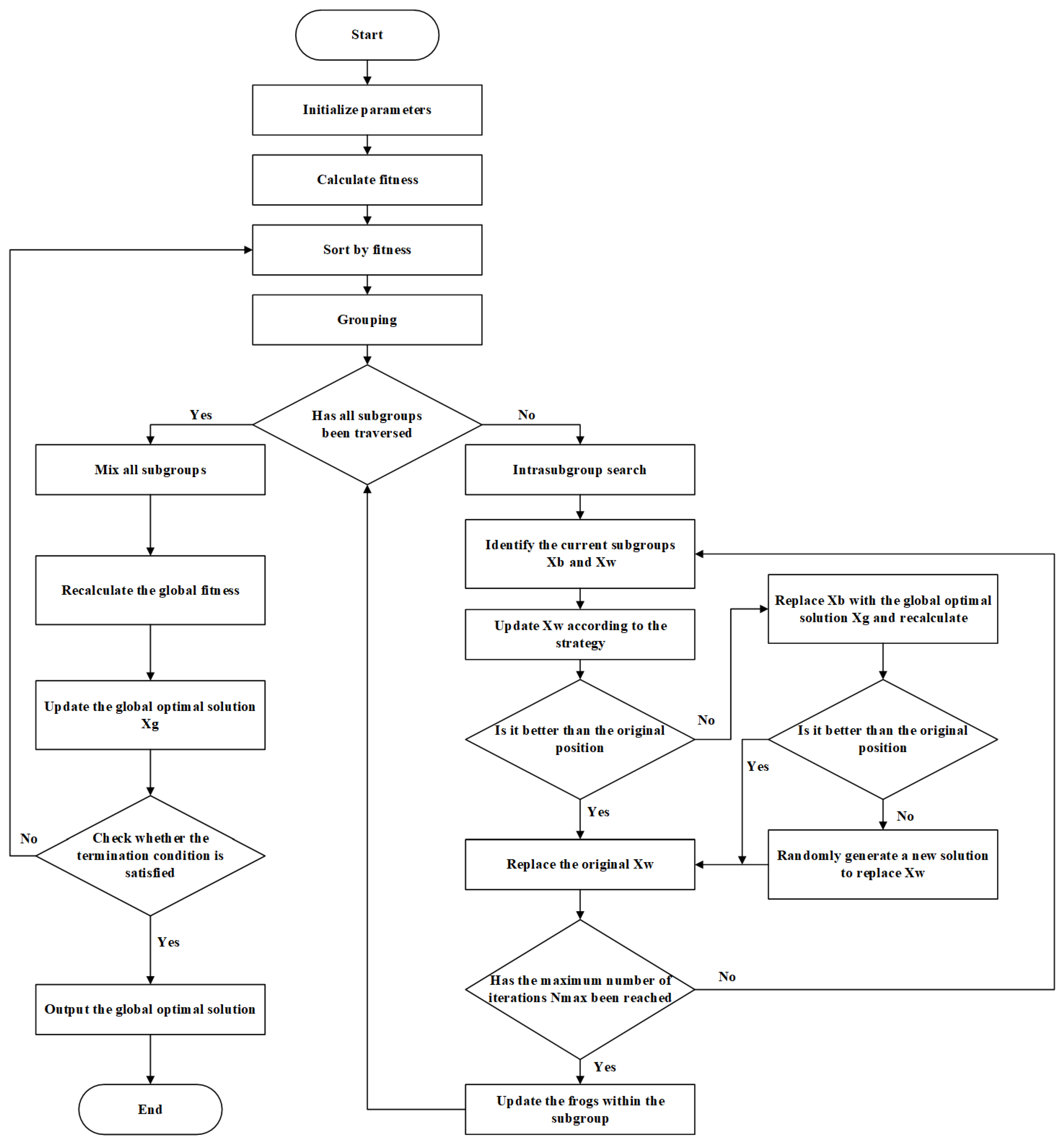
Figure 2.
Three different geoelectric models and their forward modeling results (a1~c1 are schematic diagrams of the models, a2~c2 are the forward modeling results).
Figure 2.
Three different geoelectric models and their forward modeling results (a1~c1 are schematic diagrams of the models, a2~c2 are the forward modeling results).
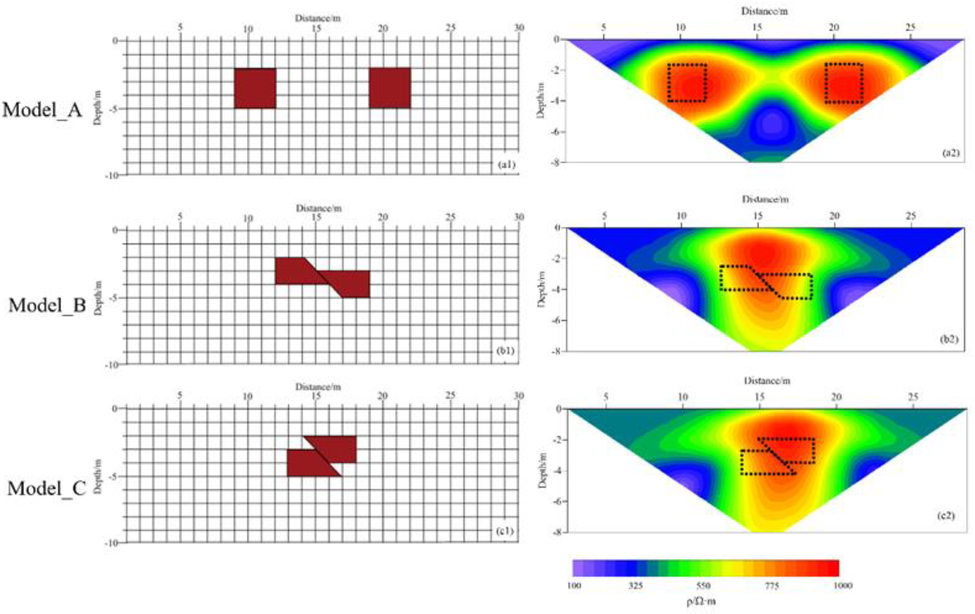
Figure 3.
Fitness Value Variation Curve of the Improved SFLA Inversion.
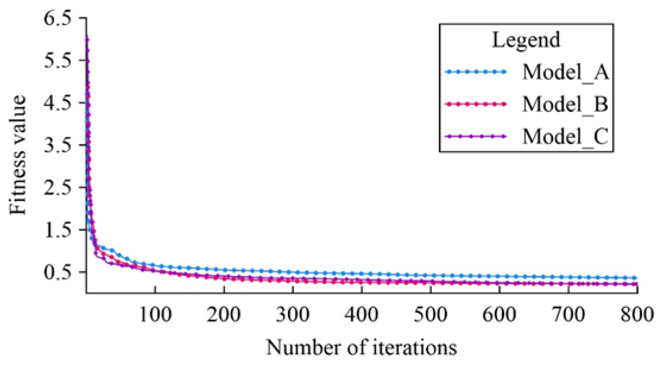
Figure 4.
Inversion results of different algorithms for three models.
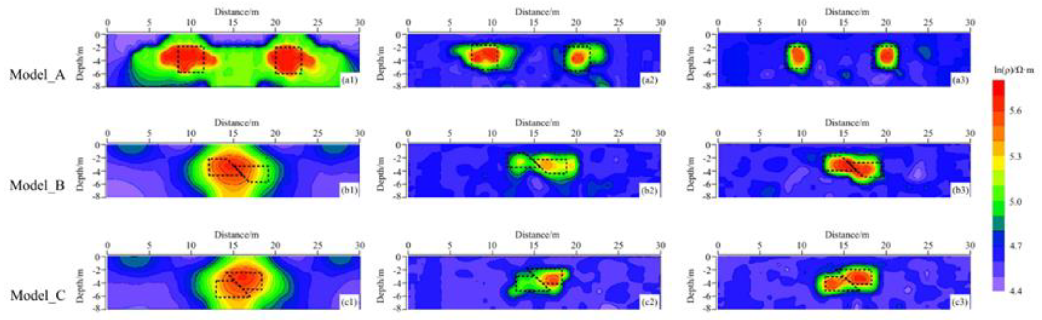
Figure 5.
Location of the study area and layout of the measurement lines.
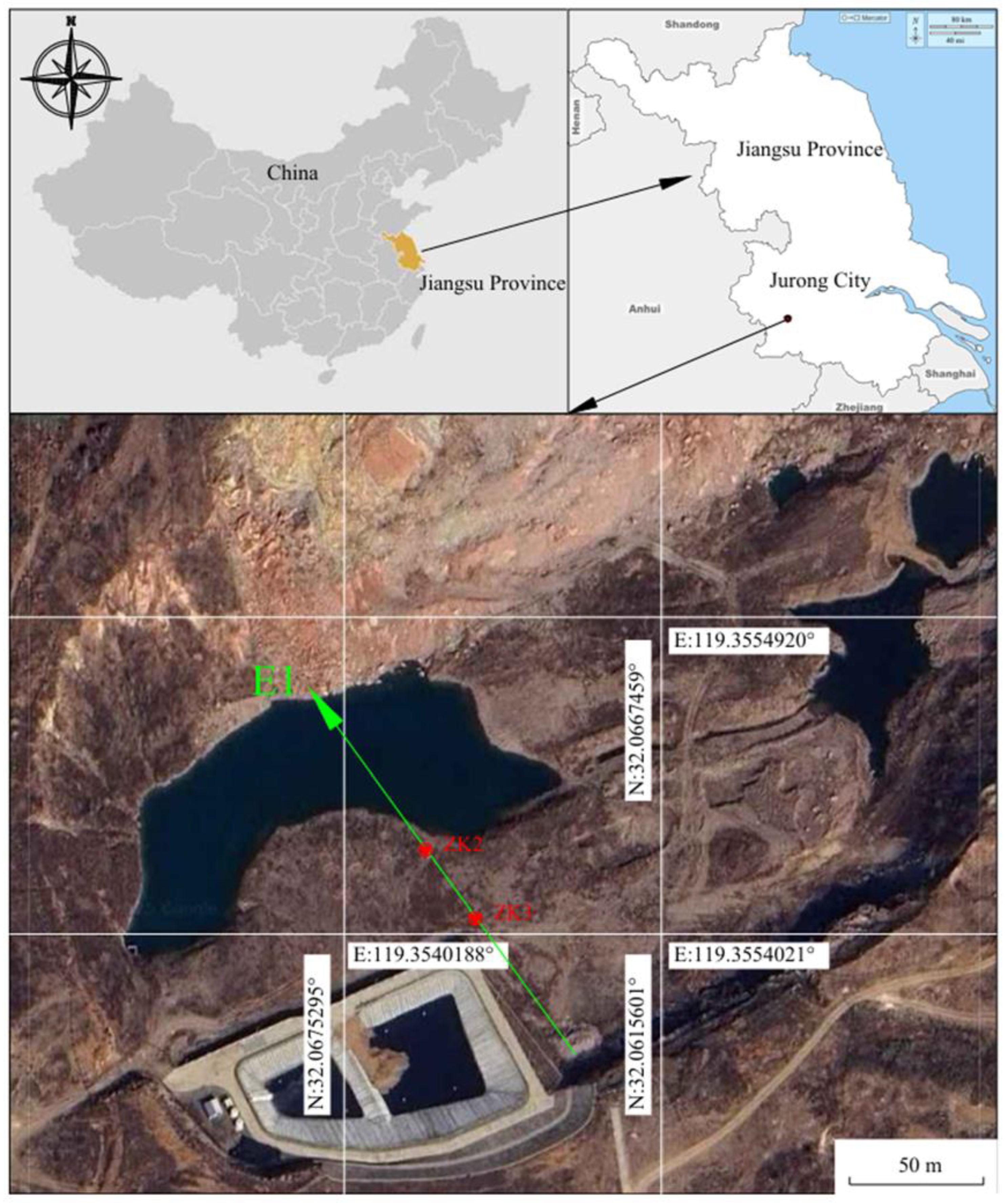
Figure 6.
Borehole ZK2 Lithological Log.
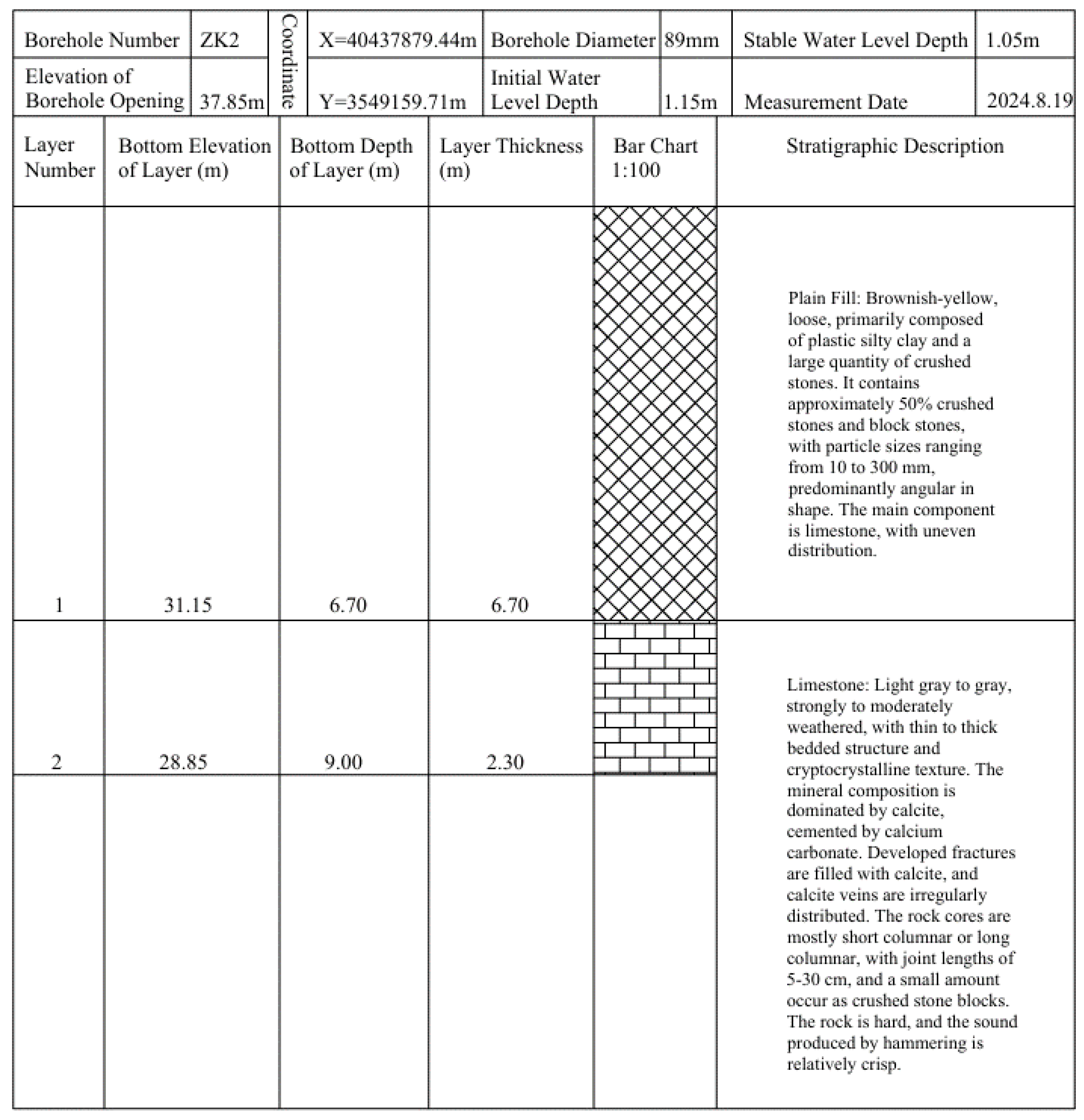
Figure 7.
Borehole ZK3 Lithological Log.
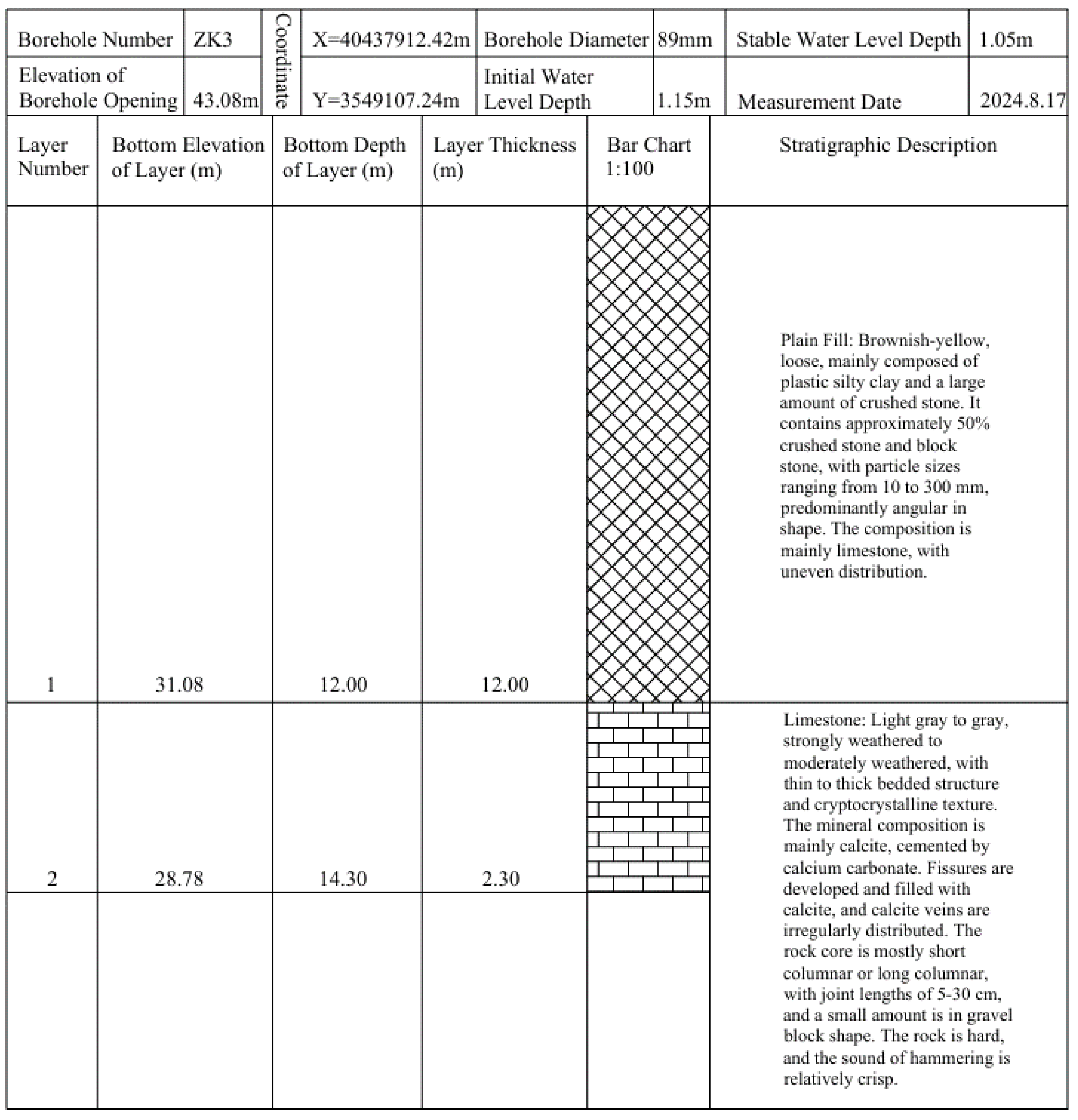
Figure 8.
Improved SFLA Inversion Fitness Variation Curve.

Figure 9.
Inversion Results of Different Algorithms for Profile E1 (a, res2dinv; b, Improved SFLA).
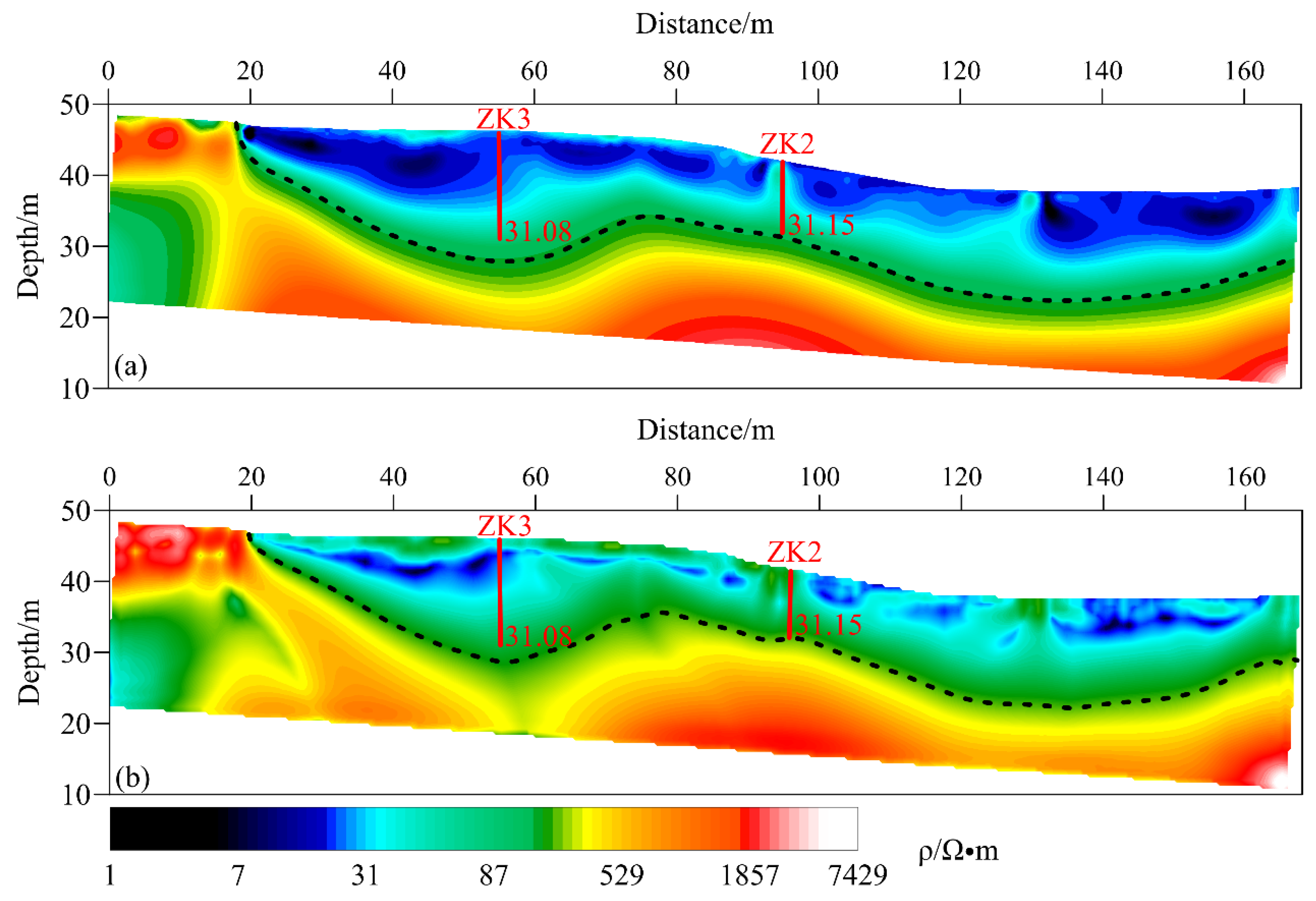

Table 1.
RMS comparison of different inversion algorithms for three models.
| Inversion algorithm | Model_A | Model_B | Model_C |
|---|---|---|---|
| The LS | 1.920 | 2.058 | 2.179 |
| The standard SFLA | 1.632 | 1.927 | 1.682 |
| The improved SFLA | 0.913 | 0.867 | 0.942 |
Disclaimer/Publisher’s Note: The statements, opinions and data contained in all publications are solely those of the individual author(s) and contributor(s) and not of MDPI and/or the editor(s). MDPI and/or the editor(s) disclaim responsibility for any injury to people or property resulting from any ideas, methods, instructions or products referred to in the content. |
© 2025 by the authors. Licensee MDPI, Basel, Switzerland. This article is an open access article distributed under the terms and conditions of the Creative Commons Attribution (CC BY) license (http://creativecommons.org/licenses/by/4.0/).
Copyright: This open access article is published under a Creative Commons CC BY 4.0 license, which permit the free download, distribution, and reuse, provided that the author and preprint are cited in any reuse.


