
Submitted:
10 February 2025
Posted:
13 February 2025
You are already at the latest version
Abstract
Subsurface geological formations are vital for validating deep engineering design assumptions, particularly in weathered terrains where unstable ground conditions pose risks. Geophysical investigations often face challenges due to inverse problem uncertainties and inadequate subsurface data. While resistivity and seismic P-wave velocity (Vp) imaging offer valuable insights, subsurface complexity necessitates integrated approaches for reliable characterization. This study introduces a machine learning-assisted geophysical–geotechnical framework combining electrical resistivity tomography, seismic refraction tomography, and borehole-based standard penetration tests (SPT-N). ML optimization metrics, including k-means clustering, PCA, Silhouette, elbow, and supervised linear regression, enhance analytical precision. A field survey over an 800 m segment in Kabota-Tawau, Sabah, Malaysia, utilized 490 collocated resistivity–Vp datasets to optimize cluster identification and interpretation accuracy. The analysis delineated four lithological units based on resistivity and Vp variations correlating with surface-subsurface properties. Clustering demonstrated strong performance, with an R² value approaching 1, a Silhouette score of 0.78, and an 88% reduction in the sum of square errors. Vulnerable zones, including weathered layers, fractures, and faults, were identified as critical for geotechnical consideration. In contrast, relatively weathered bedrock with hard-to-very-hard properties was deemed optimal for deep structural foundations requiring minimal reinforcement. This non-invasive approach enhances subsurface characterization, offering a reliable framework for construction site suitability and groundwater resource identification. It provides significant value for sedimentary regions with similar geological settings, advancing geotechnical and environmental planning.
Keywords:
Introduction
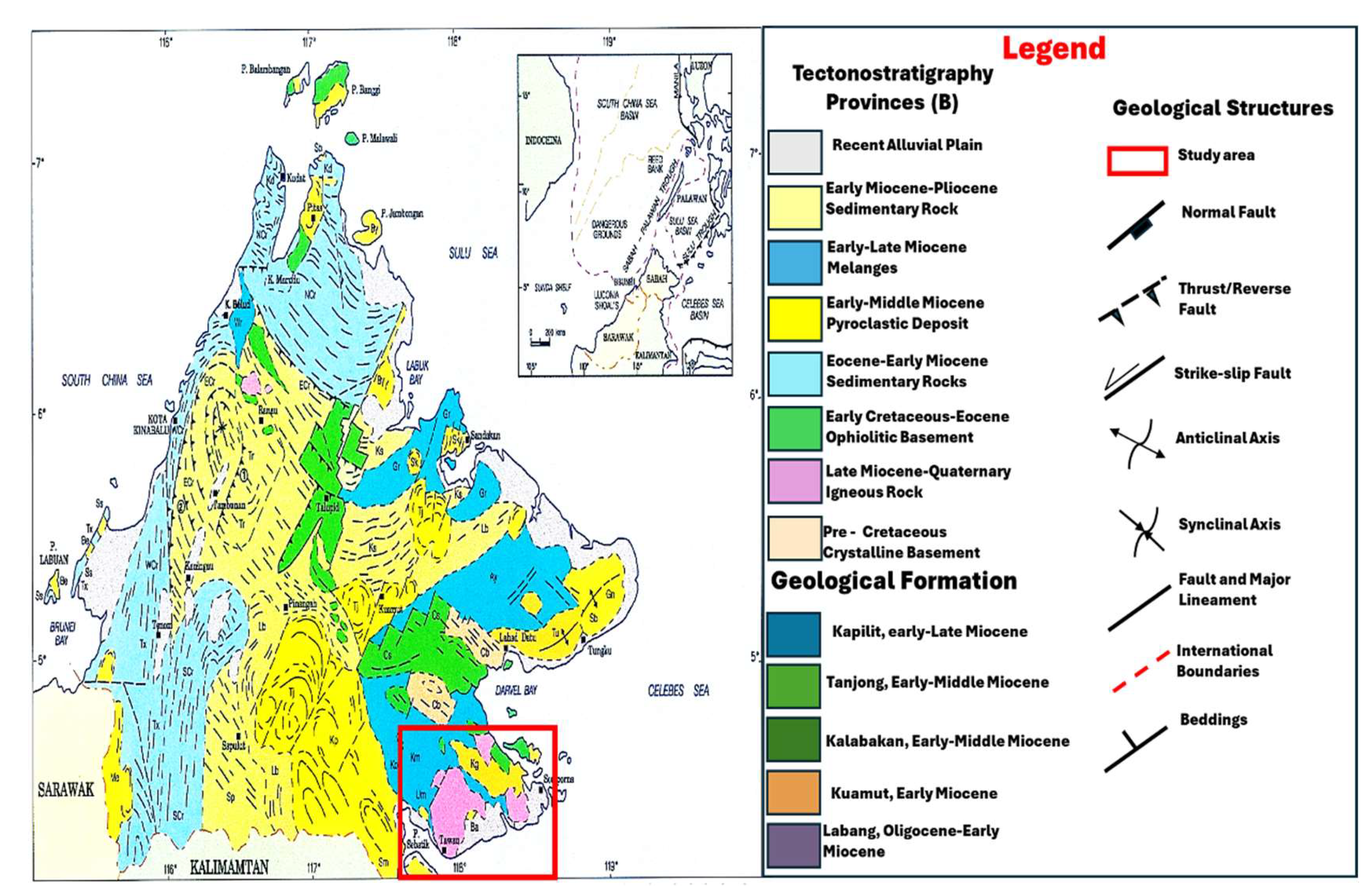
Location and Geology of the Study Area
Methodology
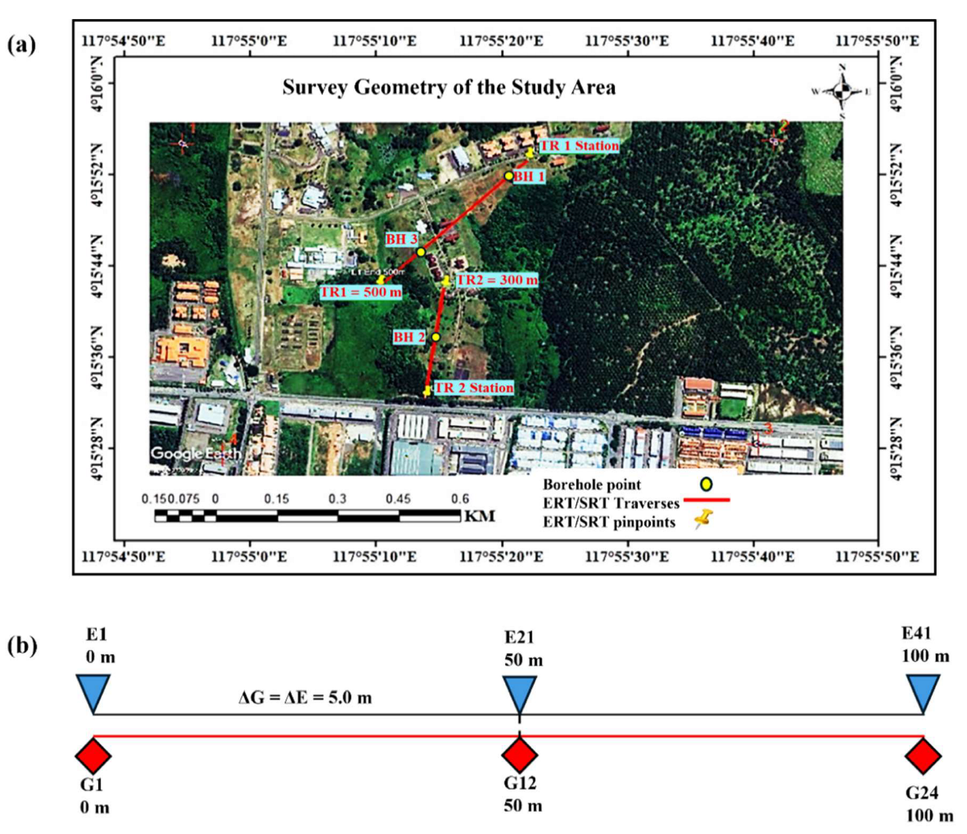
ERT and SRT Field Data Acquisition
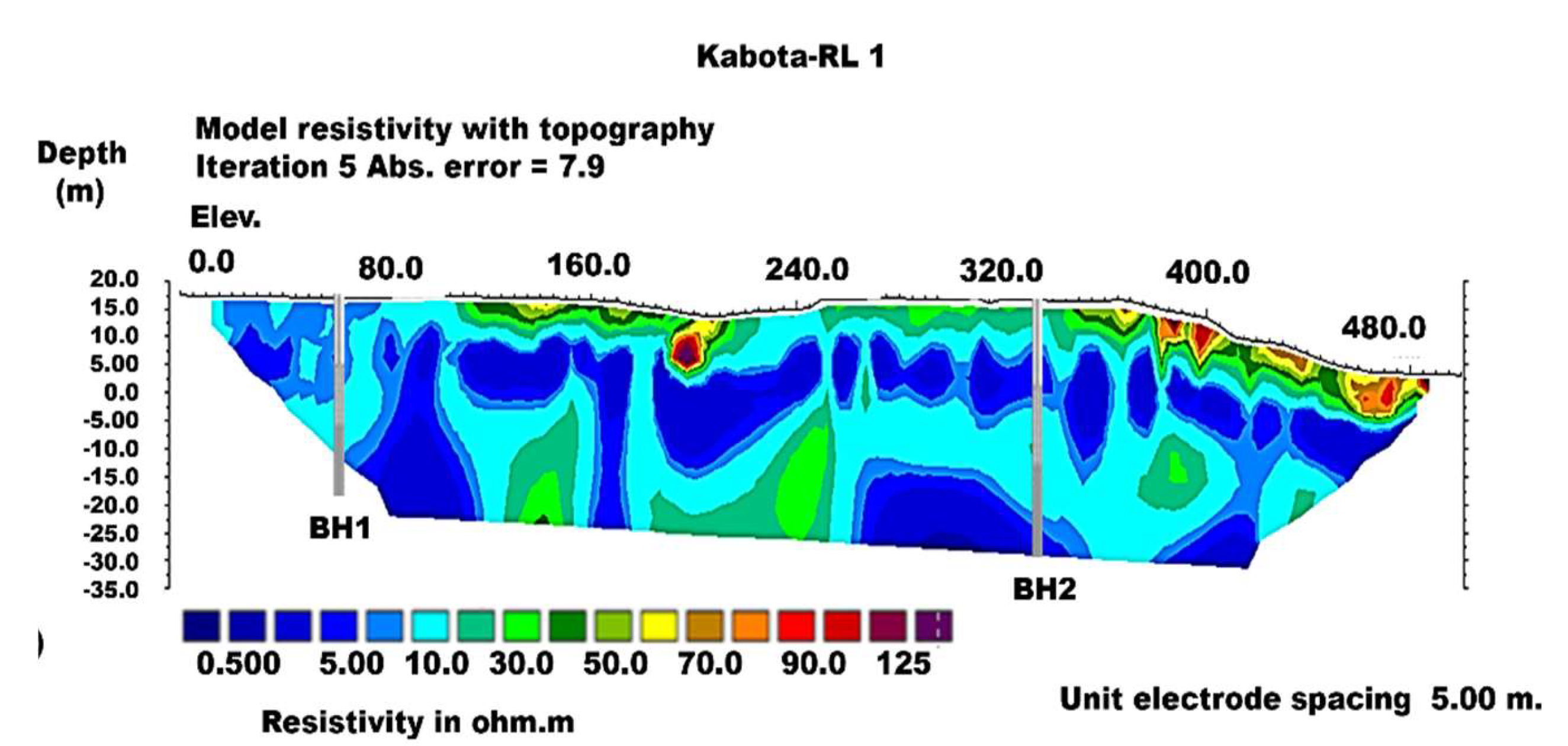
Field Data Modeling and Processing for ERT
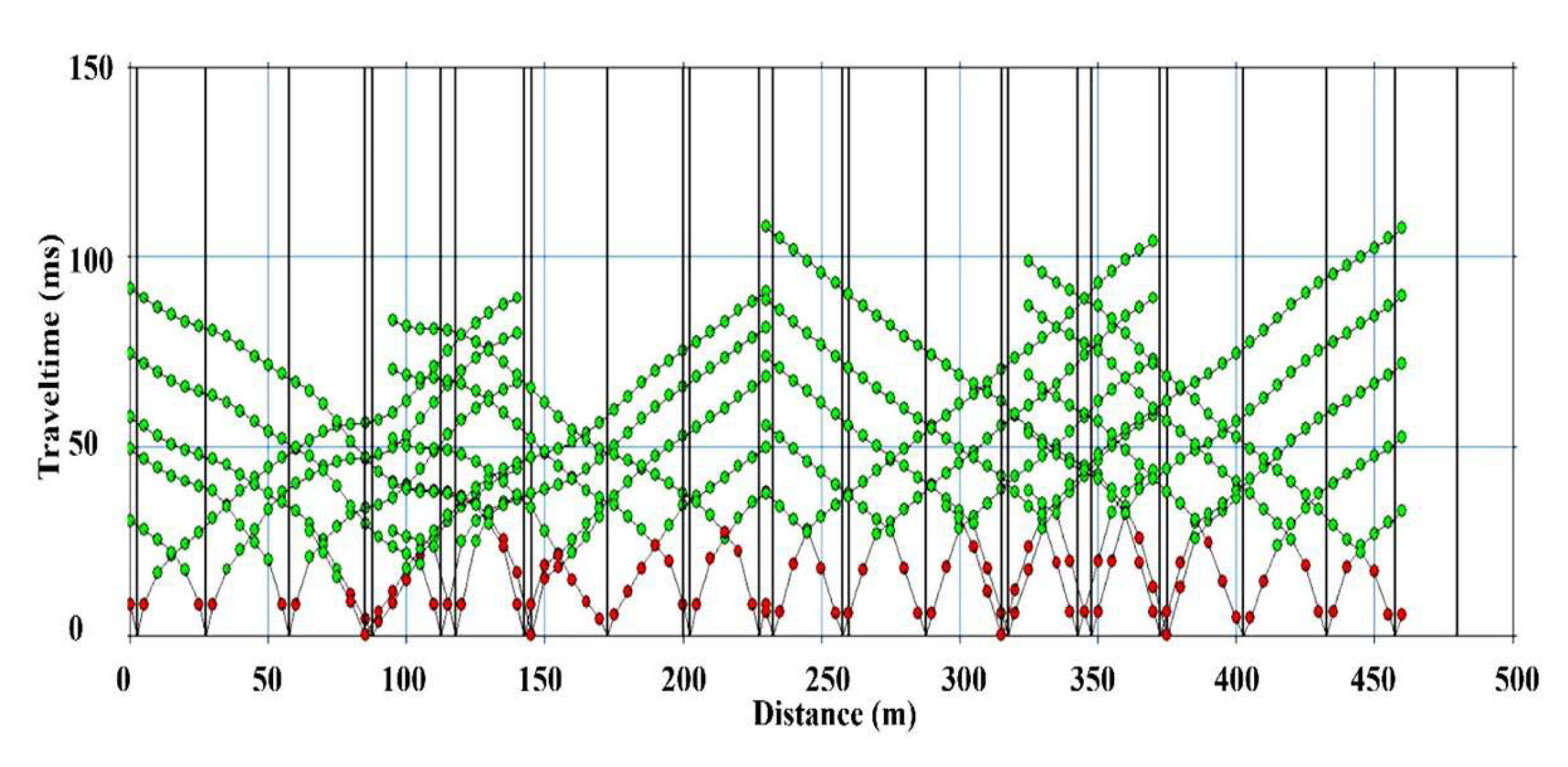
Field Data Modeling and Processing for SRT
Results
Lithological Profiles for the Assessed Boreholes
Discussion
Integrated Application of Geotomographic Analysis and k-Means Clustering
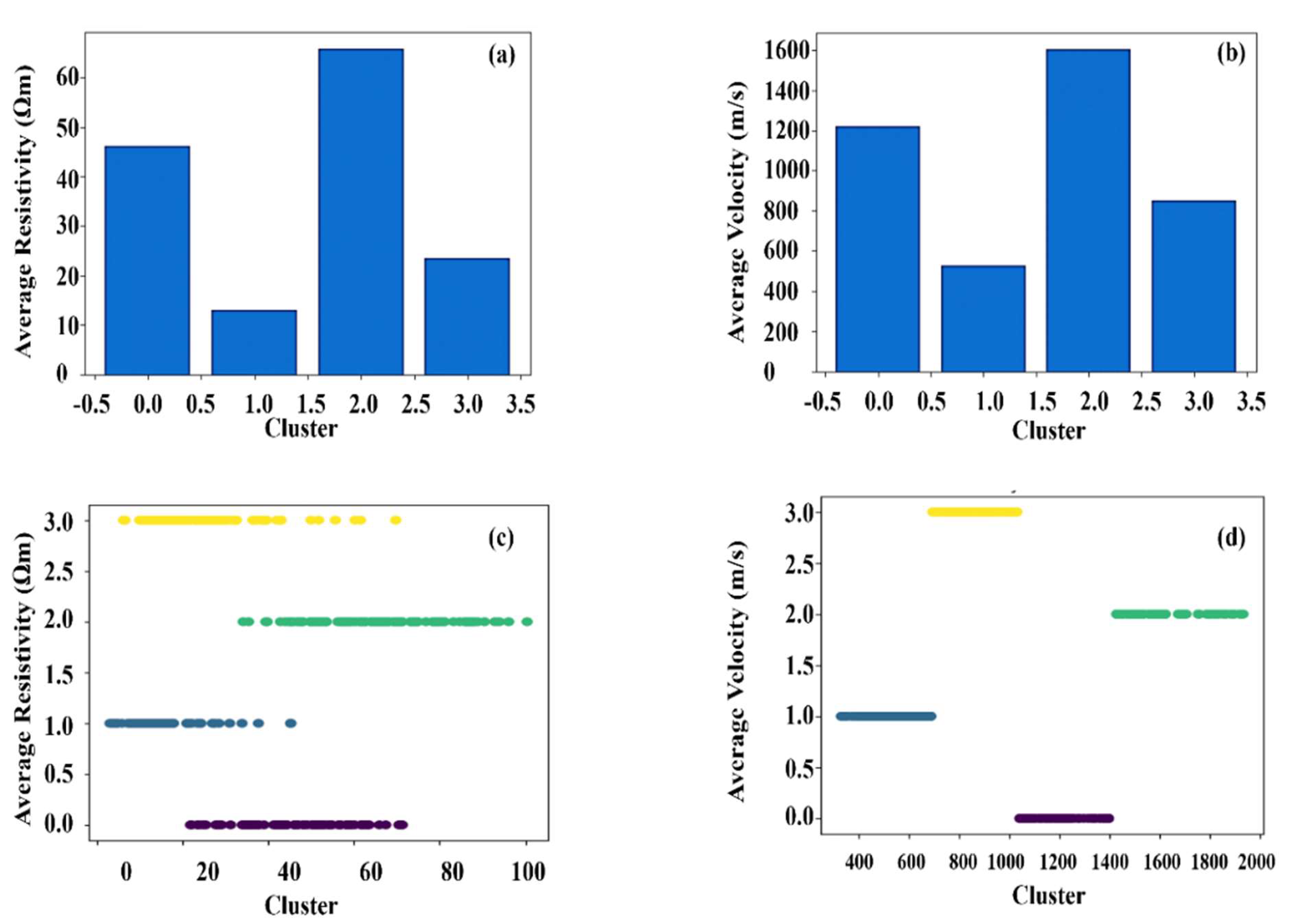
K-Mean Clustering with Validity Index
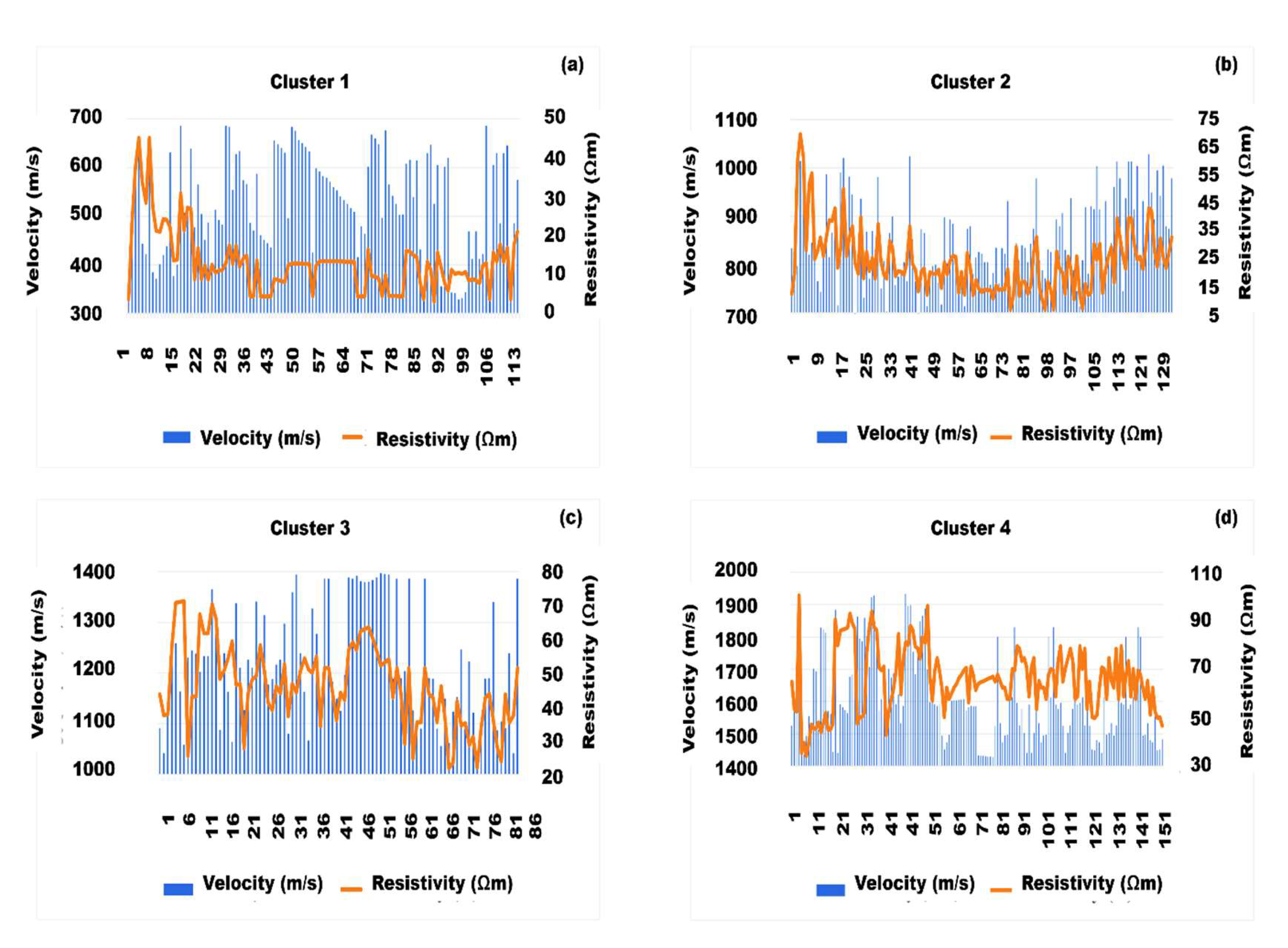
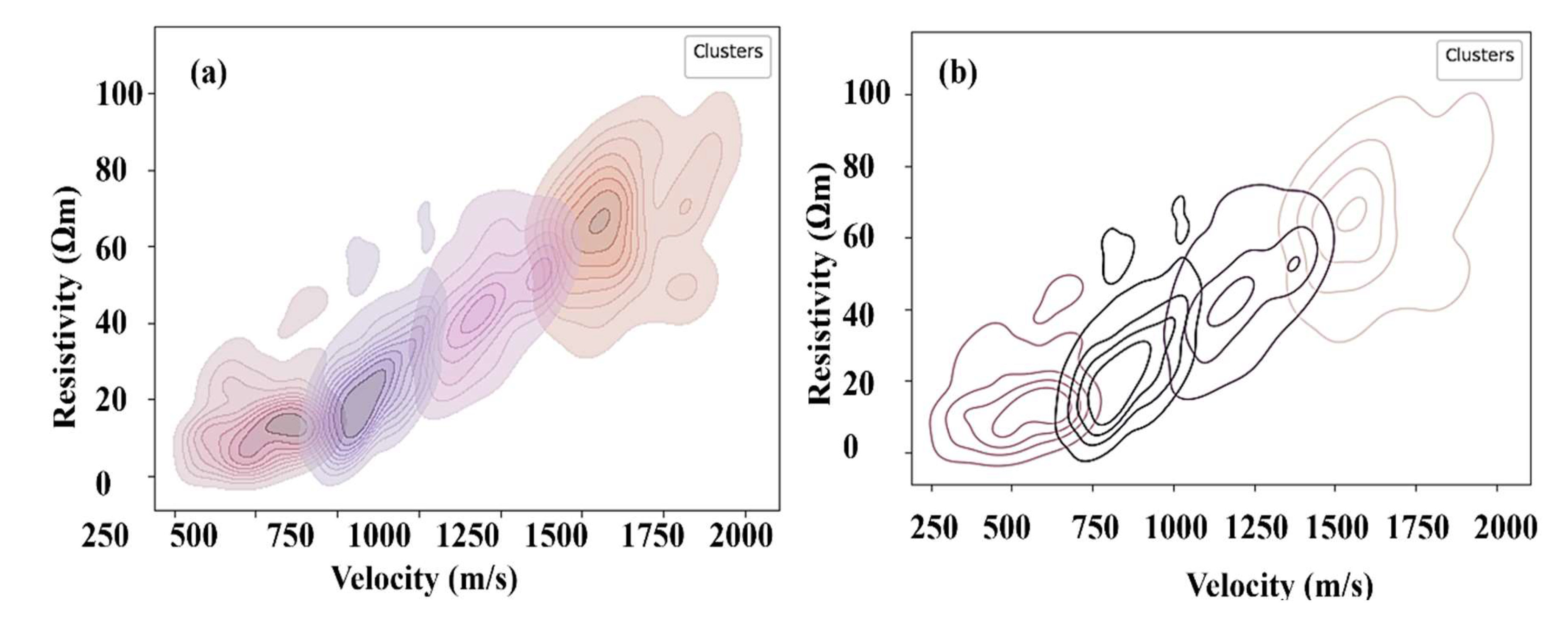
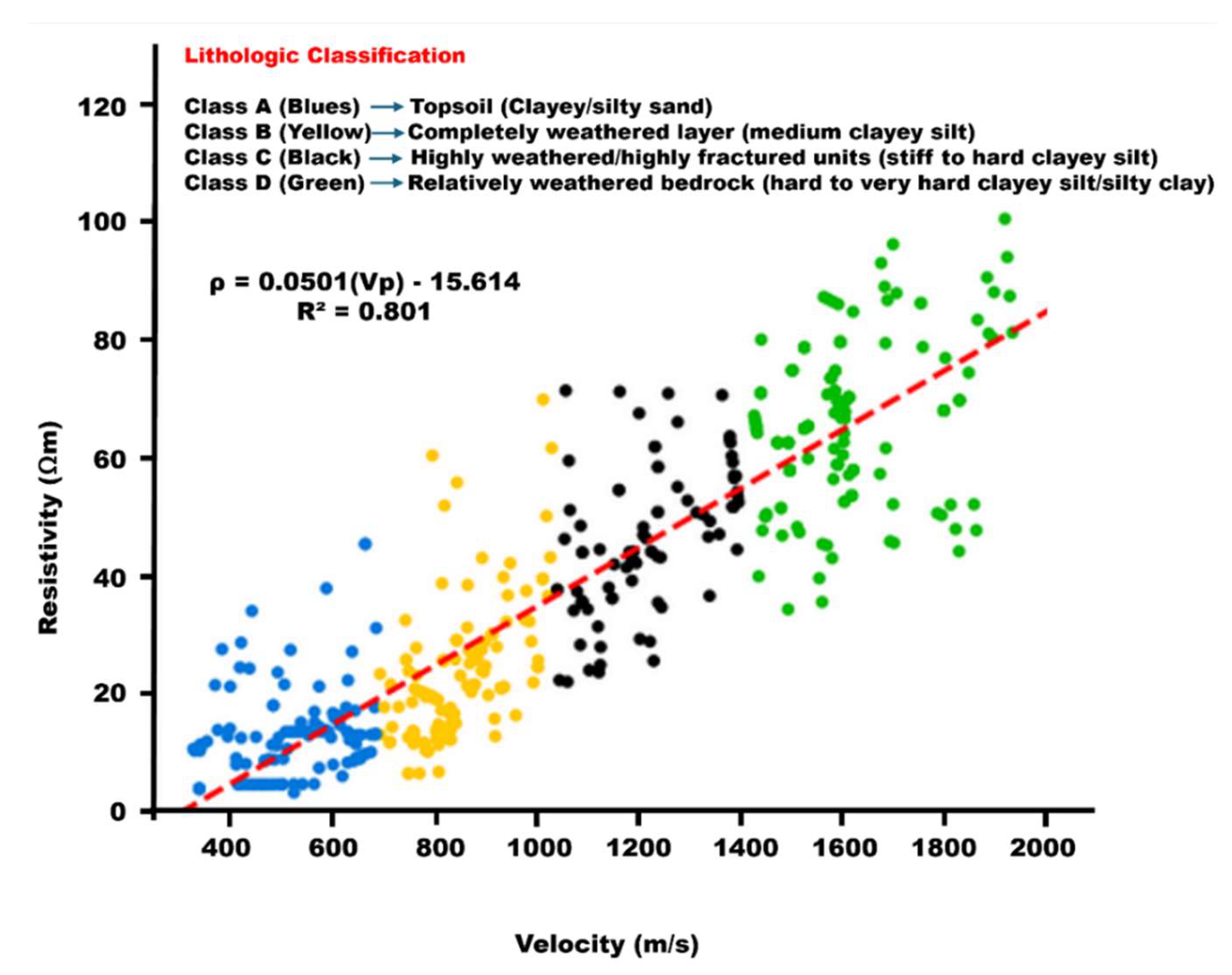
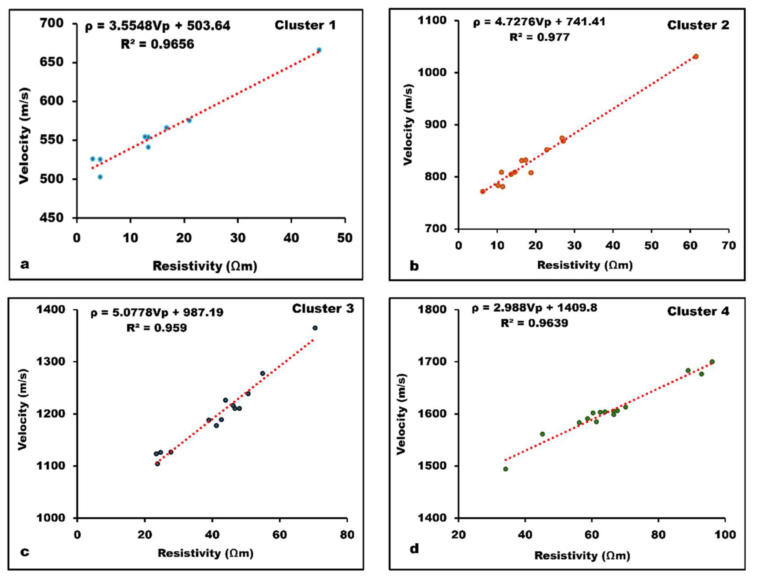
Resistivity-Vp Correlations for Identified Lithologic Units
Data availability
Author Contributions
Funding
Acknowledgments
Competing Interest
Ethical Approval
Consent to Participate
Consent to Publish
Financial interests
References
- M. U. Aka, O. E. M. U. Aka, O. E. Agbasi, O. Nsidibe Ndaraka, and O. A. Derikuma, “Assessment of Geologic Effect of Road Submergence Depths on Soil Subgrade Strength in Eket, South-South Nigeria,” Int. J. Sci. Res. Manag., vol. 10, no. 06, pp. 09–21, Jun. 2022. [Google Scholar] [CrossRef]
- A. N. Salleh et al., “Journal of Asian Earth Sciences Application of geophysical methods to evaluate soil dynamic properties in Penang Island, Malaysia,” J. Asian Earth Sci., vol. 207, no. 20, p. 104659, Mar. 20 July 2021. [CrossRef]
- A. Karpatne, I. A. Karpatne, I. Ebert-Uphoff, S. Ravela, H. A. Babaie, and V. Kumar, “Machine Learning for the Geosciences: Challenges and Opportunities,” IEEE Trans. Knowl. Data Eng., vol. 31, no. 8, pp. 1544–1554, Aug. 2019. [Google Scholar] [CrossRef]
- A. Latrach, M. L. A. Latrach, M. L. Malki, M. Morales, M. Mehana, and M. 2023. [Google Scholar] [CrossRef]
- S. Bernardinetti and P. P. G. Bruno, “The Hydrothermal System of Solfatara Crater (Campi Flegrei, Italy) Inferred From Machine Learning Algorithms,” Front. Earth Sci., vol. 7, Nov. 2019. [CrossRef]
- O. Ali and C. Sheng-Chang, “Characterization of well logs using K-mean cluster analysis,” J. Pet. Explor. Prod. Technol., vol. 10, no. 6, pp. 2245– 2256, 2020. [CrossRef]
- A. Arbelaitz, I. A. Arbelaitz, I. Gurrutxaga, J. Muguerza, J. M. Pérez, and I. Perona, “An extensive comparative study of cluster validity indices,” Pattern Recognit., vol. 46, no. 1, pp. 2013. [Google Scholar] [CrossRef]
- A. S. Akingboye, A. A. A. S. Akingboye, A. A. Bery, M. B. Aminu, M. D. Dick, G. A. Bala, and T. O. Ale, “Surface–subsurface characterization via interfaced geophysical–geotechnical and optimized regression modeling,” Model. Earth Syst. Environ., vol. 10, no. 4, pp. 5121–5143, Aug. 2024. [Google Scholar]
- B. Benjumea et al., “Undercover karst imaging using a Fuzzy c-means data clustering approach (Costa Brava, NE Spain),” Eng. Geol., vol. 293, no. 2021. [CrossRef]
- J. S. Whiteley, J. E. J. S. Whiteley, J. E. Chambers, S. Uhlemann, P. B. Wilkinson, and J. M. Kendall, “Geophysical Monitoring of Moisture-Induced Landslides: A Review,” Rev. Geophys., vol. 57, no. 1, pp. 2019. [Google Scholar] [CrossRef]
- R. Zavqiddin, Y. R. Zavqiddin, Y. Oʻgʻli, and E. Z. Abdaaliyevna, “3D Technological System of Management of Geological Exploration Processes of Mining Enterprises,” vol. 5, no. 11, pp. 254–261, 2022.
- K. Hellman, M. K. Hellman, M. Ronczka, T. Günther, M. Wennermark, C. Rücker, and T. Dahlin, “Structurally coupled inversion of ERT and refraction seismic data combined with cluster-based model integration,” J. Appl. Geophys., vol. 143, pp. 169–181, Aug. 2017. [Google Scholar] [CrossRef]
- C. V. A. LE, N. N. K. C. V. A. LE, N. N. K. NGUYEN, and T. Van NGUYEN, “Zastosowanie metody klastrowania w różnych parametrach geofizycznych do badania środowiska podpowierzchniowego,” Inżynieria Miner., vol. 1, no. 2, pp. 39–47, Jan. 2023. [Google Scholar] [CrossRef]
- M. H. Loke, J. E. M. H. Loke, J. E. Chambers, D. F. Rucker, O. Kuras, and P. B. Wilkinson, “Recent developments in the direct-current geoelectrical imaging method,” J. Appl. Geophys., vol. 95, pp. 135–156, Aug. 2013. [Google Scholar] [CrossRef]
- Z. Zeng, L. Kong, M. Wang, and H. M. Sayem, “Assessment of engineering behaviour of an intensely weathered swelling mudstone under full range of seasonal variation and the relationships among measured parameters,” Can. Geotech. J., vol. 55, no. 12, pp. 1837– 1849, 2018. [CrossRef]
- M. Hasan and Y. Shang, “Investigating the groundwater resources of weathered bedrock using an integrated geophysical approach,” Environ. Earth Sci., vol. 82, no. 9, p. 20 May; 23. [CrossRef]
- A. S. Akingboye and A. A. Bery, “Development of novel velocity–resistivity relationships for granitic terrains based on complex collocated geotomographic modeling and supervised statistical analysis,” Acta Geophys., vol. 71, no. 6, pp. 2675–2698, Mar. 2023. [CrossRef]
- E. Piegari, G. E. Piegari, G. De Donno, D. Melegari, and V. Paoletti, “A machine learning-based approach for mapping leachate contamination using geoelectrical methods,” Waste Manag., vol. 157, no. 22, pp. 121–129, Feb. 20 November 2023. [Google Scholar] [CrossRef]
- N. Zamri et al., “A comparison of unsupervised and supervised machine learning algorithms to predict water pollutions,” Procedia Comput. Sci., vol. 204, no. 2021, pp. 2022. [CrossRef]
- M. Ronczka, K. M. Ronczka, K. Hellman, T. Günther, R. Wisén, and T. Dahlin, “Electric resistivity and seismic refraction tomography: a challenging joint underwater survey at Äspö Hard Rock Laboratory,” Solid Earth, vol. 8, no. 3, pp. 671–682, Jun. 2017. [Google Scholar] [CrossRef]
- M. D. Dick, A. A. M. D. Dick, A. A. Bery, A. S. Akingboye, K. R. Ekanem, and E. Moses, “Subsurface lithological characterization via machine learning-assisted electrical resistivity and SPT-N modeling: A case study from Sabah, Malaysia,” Earth Syst. Environ. 2024. [Google Scholar]
- M. D. Dick, A. A. M. D. Dick, A. A. Bery, N. N. Okonna, K. R. Ekanem, Y. Bashir, and A. S. Akingboye, “A novel machine learning approach for interpolating seismic velocity and electrical resistivity models for early-stage soil-rock assessment,” Earth Sci. Informatics, Apr. 2024. [Google Scholar] [CrossRef]
- F. A. F. Da, C. G. Böhm, and S. P. M. Giorgi, “Petro - physical Characterization of the Shallow Sediments in a Coastal Area in NE Italy from the Integration of Active Seismic and Resistivity Data,” Surv. Geophys., no. 012345 6789, 2023. [CrossRef]
- E. James, A. A. E. James, A. A. Ghani, O. O. Akinola, and J. Asis, “Petrology and Geochemical Features of Semporna Volcanic Rocks, South-east Sabah, Malaysia,” Sains Malaysiana, vol. 50, no. 1, pp. 2021; 21. [Google Scholar] [CrossRef]
- S. Tahir, B. S. Tahir, B. Musta, and I. A. Rahim, “Geological heritage features of Tawau volcanic sequence, Sabah,” Bull. Geol. Soc. Malaysia, vol. 56, no. 56, pp. 2010; 85. [Google Scholar] [CrossRef]
- K. M. Leong, “Geological Setting of Sabah,” Petroleum Geology and Resources of Malaysia. pp. 475–497, 1999.
- C. S. Hutchison, “The North-West Borneo Trough,” Mar. Geol., vol. 271, no. 1–2, pp. 2010; 43. [CrossRef]
- R. J. Morley et al., “Sequence biostratigraphic framework for the Oligocene to Pliocene of Malaysia: High-frequency depositional cycles driven by polar glaciation,” Palaeogeogr. Palaeoclimatol. Palaeoecol., vol. 561, no. 20, p. 110058, Jan. 20 October 2021. [CrossRef]
- R. Hall, “Contraction and extension in northern Borneo driven by subduction rollback,” J. Asian Earth Sci., vol. 76, pp. 2013. [CrossRef]
- M. Madon, C. L. M. Madon, C. L. Kim, and R. Wong, “The structure and stratigraphy of deepwater Sarawak, Malaysia: Implications for tectonic evolution,” J. Asian Earth Sci., vol. 76, pp. 2013. [Google Scholar] [CrossRef]
- A. S. Akingboye and A. C. Ogunyele, “INSIGHT INTO SEISMIC REFRACTION AND ELECTRICAL RESISTIVITY TOMOGRAPHY TECHNIQUES IN SUBSURFACE INVESTIGATIONS,” Rud. Zb., vol. 34, no. 1, pp. 93–111, Feb. 2019. [CrossRef]
- M. H. Loke, “Rapid 2D resistivity forward modelling using the finite-difference and finite-element methods,” 2002.
- D. H. Griffiths and R. D. Barker, “Electrical Imaging in Archaeology,” J. Archaeol. Sci., vol. 21, no. 2, pp. 153–158, Mar. 1994. [CrossRef]
- M. H. Loke and J. W. Lane, Jr, “Inversion of Data from Electrical Resistivity Imaging Surveys in Water-Covered Areas,” Explor. Geophys., vol. 35, no. 4, pp. 266–271, Dec. 2004. [CrossRef]
- P. Kearey and M. Brooks, An introduction to geophysical exploration. 2nd edition. 1991.
- Geometrics, “SeisImager/SW TM Manual Windows Software for Analysis of Surface Waves Pickwin TM v. 4.0.1.5 WaveEq TM v. 2 Including explanation of surface wave data acquisition using Geometrics Seismodule Controller Software for ES-3000, SmartSeis ST, Geode, and Strata,” vol. 50, no. m, 2009.
- G. Software, “Golden Software (2021) Surfer User’s Guide. Golden Software, LLC. 1431 p. www.GoldenSoftware.com”.
- K. Bauer et al., “Exploring the Groß Schönebeck (Germany) geothermal site using a statistical joint interpretation of magnetotelluric and seismic tomography models,” Geothermics, vol. 39, no. 1, pp. 35–45, Mar. 2010. [CrossRef]
- S. W. Colombo D, Cogan M, Hallinan S, Mantovani M, Virgilio M, “Near-surface P-velocity modelling by integrated seismic, EM, and gravity data: examples from the middle East. 2008.
- R. D. Agustina, H. R. D. Agustina, H. Pazha, and H. Sugilar, “Identification of subsurface basement rock using geoelectrical resistivity method in development area (campus 2 UIN Sunan Gunung Djati Bandung),” IOP Conf. Ser. Mater. Sci. Eng., vol. 434, no. 2018; 1. [Google Scholar] [CrossRef]
- S. N. M. Akip Tan et al., “Correlation of Resistivity Value with Geotechnical N-Value of Sedimentary Area in Nusajaya, Johor, Malaysia,” J. Phys. Conf. Ser., vol. 995, no. 2018; 1. [CrossRef]
- C. C. Tsai, T. Kishida, and C. H. Kuo, “Unified correlation between SPT–N and shear wave velocity for a wide range of soil types considering strain-dependent behavior,” Soil Dyn. Earthq. Eng., vol. 126, no. June, p. 10 5783, 2019. [CrossRef]
- J. A. Díaz-Rodríguez, “Characterization and engineering properties of Mexico City lacustrine soils,” Proc. Int. Work. Characterisation Eng. Prop. Nat. Soils, no. February, pp. 725–755, 2003, [Online]. Available: https://s3.amazonaws.com/academia.edu.documents/40141579/Characterisation_and_engineering_propert20151118-18961-1mjkv31.pdf? 1538.
- F. Schnaid, Geocharacterisation and properties of natural soils by insitu tests, vol. 38, no. 9. 2005. [CrossRef]
- A. Burton-Johnson, C. G. A. Burton-Johnson, C. G. Macpherson, and R. Hall, “Internal structure and emplacement mechanism of composite plutons: Evidence from Mt Kinabalu, Borneo,” J. Geol. Soc. London., vol. 174, no. 1, pp. 2017. [Google Scholar] [CrossRef]
- M. N. A. Anuar, M. H. Arifin, H. Baioumy, and M. Nawawi, “A geochemical comparison between volcanic and non-volcanic hot springs from East Malaysia: Implications for their origin and geothermometry,” J. Asian Earth Sci., vol. 217, no. May, p. 10 4843, 2021. [CrossRef]
- M. G. Di Giuseppe, A. M. G. Di Giuseppe, A. Troiano, C. Troise, and G. De Natale, “k-Means clustering as tool for multivariate geophysical data analysis. An application to shallow fault zone imaging,” J. Appl. Geophys., vol. 101, pp. 108–115, Feb. 2014. [Google Scholar] [CrossRef]
- A. K. Jain, “Data clustering: 50 years beyond K-means,” Pattern Recognit. Lett., vol. 31, no. 8, pp. 651–666, Jun. 2010. [CrossRef]
- K. Sumiran, “An Overview of Data Mining Techniques and Their Application in Industrial Engineering,” Asian J. Appl. Sci. Technol., vol. 2, no. 2, pp. 947–953, 2018, [Online]. Available: www.ajast.
- S. P. Lloyd, “Least Squares Quantization in PCM,” IEEE Trans. Inf. Theory, vol. 28, no. 2, pp. 1982. [CrossRef]
- MacQueen, James and others, “Some methods for classification and analysis of multivariate observations,” Proc. fifth Berkeley Symp. Math. Stat. Probab., vol. 1, no. 14, pp. 281–297, 1967, [Online]. Available: http://books.google.de/books?
- A. Fujita, D. Y. A. Fujita, D. Y. Takahashi, and A. G. Patriota, “A non-parametric method to estimate the number of clusters,” Comput. Stat. Data Anal., vol. 73, pp. 2014; 39. [Google Scholar] [CrossRef]
- F. Batool and C. Hennig, “Clustering with the Average Silhouette Width,” Comput. Stat. Data Anal., vol. 158, p. 10 7190, 2021. [CrossRef]
- J. Singh, S. P. J. Singh, S. P. Mohanty, and D. K. Pradhan, “Introduction to SRAM,” in Robust SRAM Designs and Analysis, New York, NY: Springer New York, 2013, pp. 1–29. [CrossRef]
- A. Likas, N. A. Likas, N. Vlassis, and J. J. Verbeek, “The global k-means clustering algorithm,” Pattern Recognit., vol. 36, no. 2, pp. 2003. [Google Scholar] [CrossRef]
- A. Rajabi, M. Eskandari, M. J. Ghadi, L. Li, J. Zhang, and P. Siano, “A comparative study of clustering techniques for electrical load pattern segmentation,” Renew. Sustain. Energy Rev., vol. 120, no. November 2019, 2020. [CrossRef]
- P. Fränti and S. Sieranoja, “How much can k-means be improved by using better initialization and repeats?,” Pattern Recognit., vol. 93, pp. 2019. [CrossRef]
- R. C. De Amorim and C. Hennig, “Recovering the number of clusters in data sets with noise features using feature rescaling factors,” Inf. Sci. (Ny)., vol. 324, pp. 2015. [CrossRef]
- M. L. Lee, Y. L. M. L. Lee, Y. L. Lee, S. L. Goh, C. H. Koo, S. H. Lau, and S. Y. Chong, “Case Studies and Challenges of Implementing Geotechnical Building Information Modelling in Malaysia,” Infrastructures, vol. 6, no. 10, p. 145, Oct. 2021. [Google Scholar] [CrossRef]
- S. Sardari, M. S. Sardari, M. Eftekhari, and F. Afsari, “Hesitant fuzzy decision tree approach for highly imbalanced data classification,” Appl. Soft Comput. J., vol. 61, pp. 2017. [Google Scholar] [CrossRef]
- K. Husain, M.R.; Ishak, A.M., Redzuan, N., Kalken, T.V., Eds.; Brown, “Malaysian national water balance system (NAWABS) for improved river basin management: Case study in the Muda River basin.,” in In Proceedings of the 37th IAHR World Congress, Kuala Lumpur, Malaysia, 1, 2017. [Google Scholar]
- M. Ramze Rezaee, B. P. F. M. Ramze Rezaee, B. P. F. Lelieveldt, and J. H. C. Reiber, “A new cluster validity index for the fuzzy c-mean,” Pattern Recognit. Lett., vol. 19, no. 3–4, pp. 1998. [Google Scholar] [CrossRef]
- T. Bohlin, “Validation techniques,” in Interactive System Identification: Prospects and Pitfalls, Berlin, Heidelberg: Springer Berlin Heidelberg, 1991, pp. 220–243. [CrossRef]
- J. Saha and J. Mukherjee, “CNAK: Cluster number assisted K-means,” Pattern Recognit., vol. 110, p. 10 7625, 2021. [CrossRef]
- P. Govender and V. Sivakumar, “Application of k-means and hierarchical clustering techniques for analysis of air pollution: A review (1980–2019),” Atmos. Pollut. Res., vol. 11, no. 1, pp. 2020; 56. [CrossRef]
- M. Halkidi, M. M. Halkidi, M. Vazirgiannis, and Y. Batistakis, “Quality Scheme Assessment in the Clustering Process,” in Lecture Notes in Computer Science (including subseries Lecture Notes in Artificial Intelligence and Lecture Notes in Bioinformatics), 2000, pp. 265–276. [CrossRef]
- R. Ünlü and P. Xanthopoulos, “Estimating the number of clusters in a dataset via consensus clustering,” Expert Syst. Appl., vol. 125, pp. 2019; 39. [CrossRef]
- Y. Liu, Z. Y. Liu, Z. Li, H. Xiong, X. Gao, and J. Wu, “Understanding of internal clustering validation measures,” Proc. - IEEE Int. Conf. Data Mining, ICDM, pp. 2010. [Google Scholar] [CrossRef]
- E. Rendón, I. E. Rendón, I. Abundez, A. Arizmendi, and E. M. Quiroz, “Internal versus External cluster validation indexes,” Int. J. Comput. Commun., vol. 5, no. 1, pp. 27--34, 2011, [Online]. Available: http://w.naun.org/multimedia/UPress/cc/20-463.
- P. J. Rousseeuw, “Silhouettes: A graphical aid to the interpretation and validation of cluster analysis,” J. Comput. Appl. Math., vol. 20, no. C, pp. 1987; 65. [CrossRef]
- L. Ge et al., “Current Trends and Perspectives of Detection and Location for Buried Non-Metallic Pipelines,” Chinese J. Mech. Eng. (English Ed., vol. 34, no. 2021; 1. [CrossRef]
- A. Pérez-López, M. A. Pérez-López, M. García-López, and M. González-Gil, “Integrated Interpretation of Electrical Resistivity Tomography for Evaporite Rock Exploration: A Case Study of the Messinian Gypsum in the Sorbas Basin (Almería, Spain),” Minerals, vol. 13, no. 2023; 2. [Google Scholar] [CrossRef]
- A. Hegde and A. Anand, “Resistivity Correlations with SPT-N and Shear Wave Velocity for Patna Soil in India,” Indian Geotech. J., vol. 52, no. 1, pp. 2022. [CrossRef]
- M. Hasan and Y. Shang, “Geophysical evaluation of geological model uncertainty for infrastructure design and groundwater assessments,” Eng. Geol., vol. 299, p. 106560, Mar. 2022. [CrossRef]
- B. Balarabe and A. A. Bery, “Modeling of soil shear strength using multiple linear regression (MLR) at Penang, Malaysia,” J. Eng. Res., vol. 9, no. 3A, pp. 40–51, Sep. 2021. [CrossRef]
- D. Colombo and T. Keho, “The non-seismic data and joint inversion strategy for the near surface solution in Saudi Arabia,” in SEG Technical Program Expanded Abstracts 2010, Society of Exploration Geophysicists, Jan. 2010, pp. 1934–1938. [CrossRef]
- G. M. Deynoux, M. G. M. Deynoux, M., Miller, J. M. G., Domack, E. W., Eyles, N., Fairchild, I. J., & Young, “Earth’s glacial record,” in Glaciers, Cambridge University Press, 2004, pp. 303–334. [CrossRef]
- K. A. Hatta and S. B. A. Syed Osman, “Correlation of Electrical Resistivity and SPT-N Value from Standard Penetration Test (SPT) of Sandy Soil,” Appl. Mech. Mater., vol. 785, pp. 702–706, Aug. 2015. [CrossRef]
- J. T. D. Gonçalves, M. A. B. J. T. D. Gonçalves, M. A. B. Botelho, S. L. Machado, and L. G. Netto, “Correlation between field electrical resistivity and geotechnical SPT blow counts at tropical soils in Brazil,” Environ. Challenges, vol. 5, no. 2021. [Google Scholar] [CrossRef]
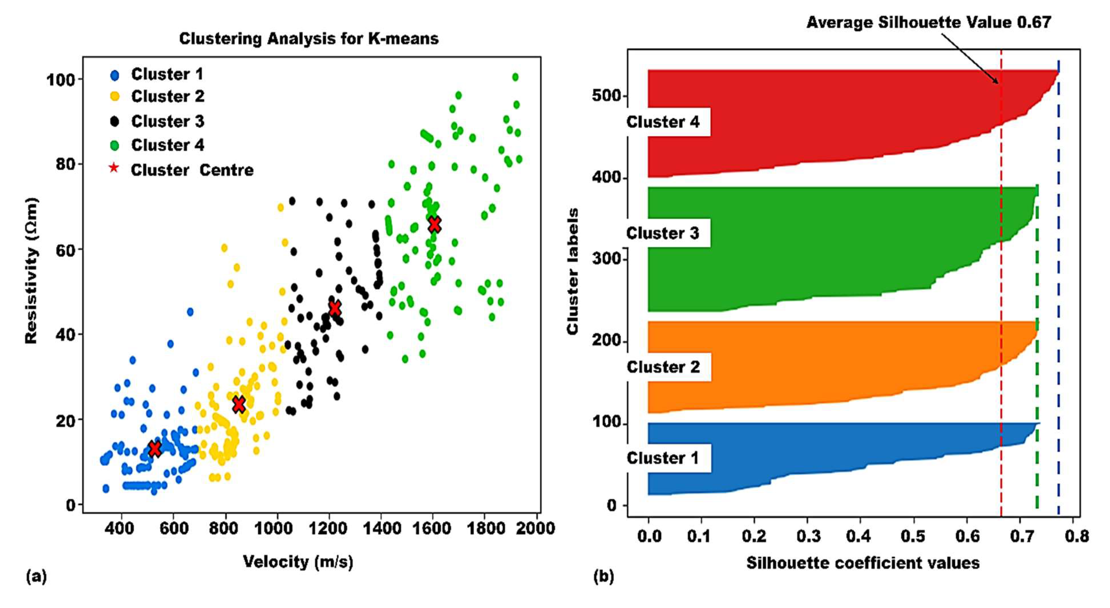

| Number of clusters (k) | Vp Centroids (m/s) | Resistivity Centroids (Ωm) | Silhouette value for each cluster |
|---|---|---|---|
| 1 (Blue) | 529.02 | 13.13 | 0.74 |
| 2 (Yellow) | 851.86 | 23.58 | 0.75 |
| 3 (Black) | 1221.50 | 46.11 | 0.74 |
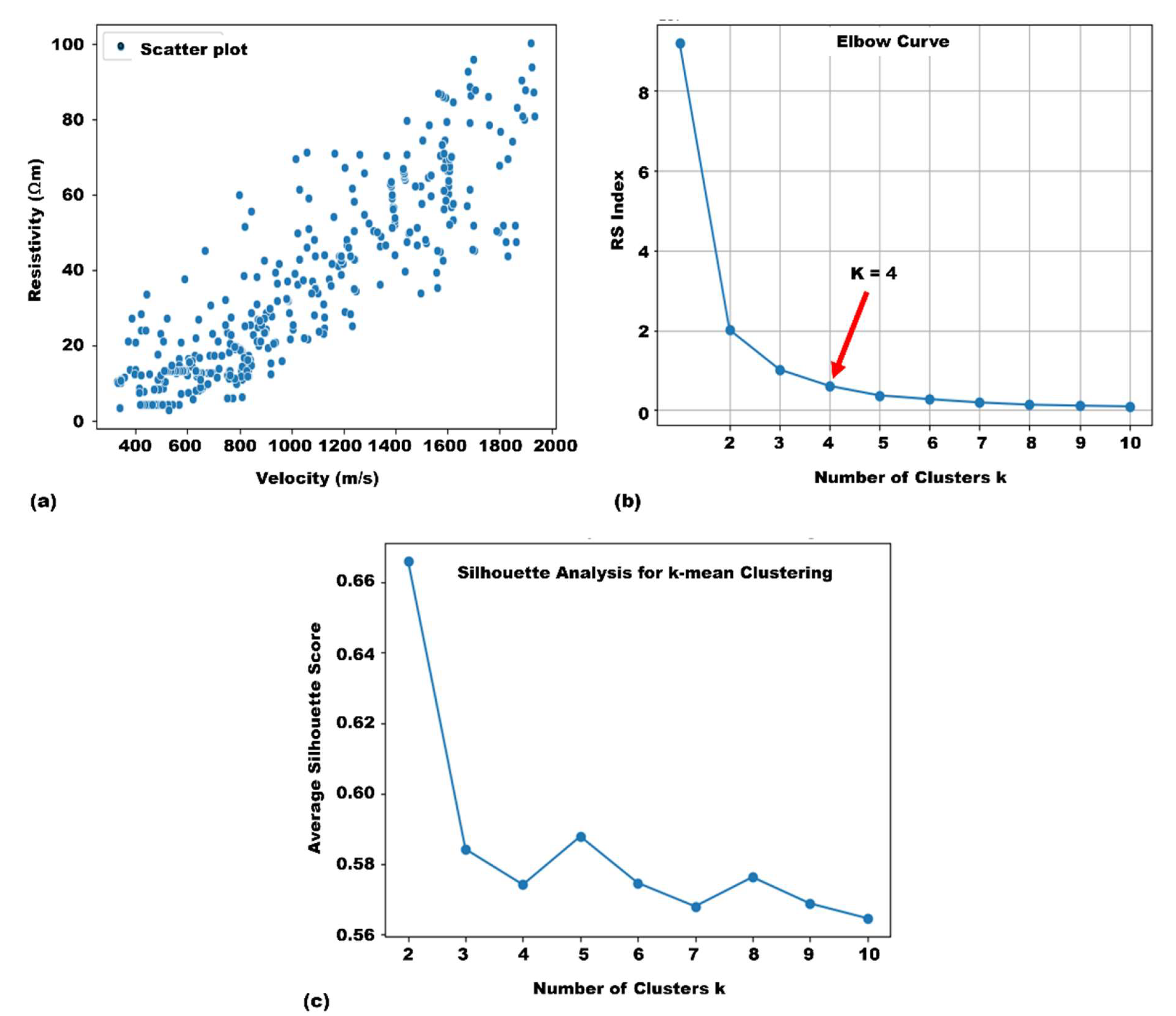
| 4 (Green) | 1604.95 | 65.89 | 0.78 |
| Silhouette score for k | Average Silhouette score for k | WCSS (or SSE)x107 | %change of SSE |
|---|---|---|---|
| 2 | 0.58 | 2.01 | --- |
| 3 | 0.57 | 102 | 98.01 |
| 4 | 0.67 | 9.21 | 88.96 |
| 5 | 0.59 | 6.05 | 1420.69 |
| 6 | 0.58 | 3.68 | 64.33 |
| Cluster | Vp centroids | Resistivity centroids | Range of ρvalues (Ωm) | Range of Vpvalues (m/s) | Lithological units |
|---|---|---|---|---|---|
| 1 | 529.02 | 13.13 | 0.5–20 | <100–700 | topsoil (clayey silt) |
| 2 | 851.86 | 23.58 | 5–30 | 700–1100 | completely weathered soil unit (medium-stiff clayey silt) |
| 3 | 1221.50 | 46.11 | 30–50 | 1100–1400 | highly weathered/fractured units (very stiff to hard clayey silt) |
| 4 | 1604.95 | 65.89 | 50 to >125 | 1400 to >1900 | relatively weathered/fractured units (hard to very hard clayey silt) |
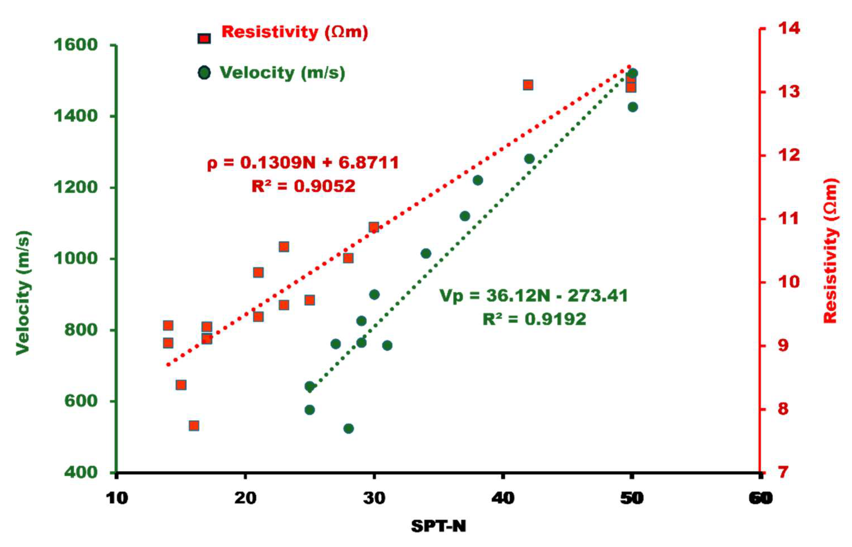
| S/N | Velocity (Vp) (m/s) | Resistivity (Ωm) | ||||||
|---|---|---|---|---|---|---|---|---|
| SPT (N) | Obs. Vp (m/s) | Pred. Vp (m/s) | Percentage Matching | SPT (N) | Observed Resistivity (Ωm) | Predicted Resistivity (Ωm) | Percentage Matching (%) | |
| 1 | 30 | 899.55 | 810.19 | 90.07 | 14 | 9.3154 | 8.7037 | 93.4335 |
| 2 | 29 | 825.58 | 774.07 | 93.76 | 17 | 9.1196 | 9.0964 | 99.7456 |
| 3 | 50 | 1520.34 | 1532.59 | 100.81 | 17 | 9.1056 | 9.0964 | 99.8990 |
| 4 | 27 | 760.86 | 701.83 | 92.24 | 30 | 10.8702 | 10.7981 | 99.3367 |
| 5 | 25 | 641.99 | 629.59 | 98.07 | 42 | 13.1114 | 12.3689 | 94.3369 |
| Lithologic units/Clusters | Range of Vp values (m/s) | Range of ρ values (Ωm) | R2 values | Engineering Implication |
|---|---|---|---|---|
| Cluster 1: Topsoil (Clayey/silty sand) | <100–700 | 0–20 | 0.9656 | Unconsolidated lithology which is unsuitable for engineering structures |
| Cluster 2: Completely weathered layer (medium clayey silt) | 700–1100 | 5– 30 | 0.9770 | Not ideal for extensive construction projects; moderate compaction is recommended for lighter structures with enhanced reinforcement. |
| Cluster 3: Highly weathered/highly fractured units (stiff to hard clayey silt) | 1100–1400 | 30–50 | 0.9590 | Moderate compaction is needed, along with excavation of loose soils and sealing water paths, to strengthen the load-bearing capacity. |
| Cluster 4: Relatively weathered bedrock (hard to very hard clayey silt/silty clay) | 1400 to >1900 | 50 to >125 | 0.9639 | Well-compacted, making the layer more reliable for supporting heavy loads, complex, and stable structures. Sealing continuous water sections further improves load-bearing capacity. |
Disclaimer/Publisher’s Note: The statements, opinions and data contained in all publications are solely those of the individual author(s) and contributor(s) and not of MDPI and/or the editor(s). MDPI and/or the editor(s) disclaim responsibility for any injury to people or property resulting from any ideas, methods, instructions or products referred to in the content. |
© 2025 by the authors. Licensee MDPI, Basel, Switzerland. This article is an open access article distributed under the terms and conditions of the Creative Commons Attribution (CC BY) license (http://creativecommons.org/licenses/by/4.0/).


