
Submitted:
12 May 2025
Posted:
13 May 2025
You are already at the latest version
Abstract
Detecting underground cavities using gravity measurements is a challenging inverse problem characterized by non-uniqueness, instability, and sensitivity to noise. Classical inversion approaches based on domain discretization often lead to highly underdetermined problems that require strong regularization. In this work, we propose a model reduction strategy that represents subsurface cavities as prolate ellipsoids embedded in a homogeneous background, significantly reducing the number of free parameters and improving computational efficiency. The inverse problem is solved using Particle Swarm Optimization (PSO), which allows both optimization and thorough exploration of the parameter space, enabling direct uncertainty quantification without the need for explicit regularization. Synthetic experiments with added Gaussian noise demonstrate that the method accurately recovers the location, size, orientation, and density contrast of anomalies, while capturing the anisotropic nature of model uncertainty. A synthetic case study simulating water-filled karstic cavities is also presented to illustrate the method’s potential for realistic scenarios. The results underscore the advantages of combining geometric model reduction with swarm-based global optimization in gravity inversion, particularly when model simplicity, computational efficiency, and uncertainty assessment are critical.
Keywords:
Gravity inversion
; uncertainty quantification
; model reduction
; ellipsoidal parameterization
; Particle Swarm Optimization
; anomaly detection
1. Introduction
Inverse problems in gravimetry aim to infer the geometry and physical properties of subsurface structures from gravity measurements collected at the surface. These problems are inherently ill-posed in the sense of Hadamard [1], often exhibiting non-uniqueness, instability, and sensitivity to noise due to the smoothing nature of gravity data [2,3]. As multiple models can equally explain the observations, the inversion process is typically ambiguous and requires additional constraints to stabilize the solutions [4].
Classical inversion techniques address these challenges by incorporating regularization strategies, typically following the frameworks established by Tikhonov and further formalized by Menke [5] and Aster et al. [6]. However, the choice of regularization parameters and reference models can significantly influence the final solution, potentially introducing biases or masking important geological features [7,8]. Furthermore, the topography of the misfit functional in both linear and nonlinear inverse problems is often characterized by multiple minima and complex structures [4,8], making the inversion process even more delicate.
Probabilistic approaches, particularly those grounded in Bayesian inference [8], have been proposed to better capture the inherent uncertainties of inverse problems. Techniques such as Monte Carlo sampling [9,10] and transdimensional methods [8,11] allow for a more rigorous exploration of the solution space but at the cost of increased computational demands. Parsimonious approaches to Bayesian inversion have also been explored to balance complexity and tractability [9].
In gravity inversion, model reduction strategies have emerged as an effective alternative to full-space discretizations. Instead of parameterizing the subsurface with finely meshed grids, model reduction uses simple geometric bodies, such as prisms, spheres, cylinders, or ellipsoids, to describe anomalies with a small number of parameters [7,12]. These methods reduce the dimensionality of the problem and mitigate the curse of dimensionality effects [13], while often preserving key geological realism. Among model reduction strategies, ellipsoidal parameterization provides an advantageous balance between simplicity and flexibility. By representing subsurface cavities or density anomalies as ellipsoids, it is possible to capture variations in depth, orientation, and elongation, while maintaining analytical or semi-analytical expressions for forward modeling [12,14].
Global optimization algorithms, particularly Particle Swarm Optimization (PSO) [15,16], have proven highly effective for solving inverse problems characterized by complex, multimodal objective functions. PSO-based approaches allow not only the search for optimal solutions but also the sampling of plausible models, facilitating uncertainty quantification without relying on explicit regularization [17,18,19]. Applications of PSO to gravity inversion problems have been successfully demonstrated in various geological contexts [17,20,21,22]. Additionally, recent advances have explored the integration of PSO with Bayesian ideas for model space exploration [8], transdimensional approaches [11], and hybrid strategies to improve the robustness of inversion results in noisy environments [23].
In this study, we address the detection and characterization of anomalous bodies by representing them as prolate ellipsoids embedded in a homogeneous background. Assuming the density contrast is known, the model is defined by seven parameters: the coordinates of the ellipsoid center, the lengths of two semi-axes, the azimuth, and the tilt. We solve the inverse problem using PSO, with an emphasis on simultaneously achieving optimization and uncertainty quantification. We try also to introduce the density contrast as an additional parameter to estimate.
The proposed methodology is validated through synthetic experiments contaminated with Gaussian noise. The results demonstrate that ellipsoidal model reduction combined with swarm-based global optimization provides an efficient, robust, and interpretable framework for gravity inversion problems where the assessment of uncertainty is critical.
The rest of this article is structured as follows: Section 2 introduces the mathematical and computational framework. Sections 3 and 4 presents inversion results from synthetic noisy datasets. Section 5 discusses the implications and performance of the method. Section 6 offers conclusions and future research directions.
2. Materials and Methods
We consider the forward problem of computing the gravity anomaly produced by an ellipsoidal body with known density contrast embedded in a homogeneous background. The corresponding inverse problem consists of estimating the model parameters—position, size, orientation, and density contrast—from a finite set of surface gravity measurements. Due to the fact that gravity derives from a potential field, the limited number of observations, and the presence of measurement noise, the problem is ill-posed: its solution is generally non-unique and unstable [1,3]. The objective function associated with this inverse problem exhibits a highly irregular, non-convex landscape characterized by multiple local minima and flat regions. Even simple gravimetric configurations can produce highly complex misfit surfaces, as demonstrated by [4], which limits the effectiveness of local gradient-based optimization methods. To address these challenges, we adopt a model reduction strategy by parameterizing each anomaly as a prolate ellipsoid. The model vector includes eight parameters per body: center coordinates , semi-major and semi-minor axis lengths , azimuth , tilt angle , and density contrast . This results in a compact parameterization of dimension , where denotes the number of anomalous bodies. The gravitational response of each ellipsoid is computed analytically using the formulation of MacMillan [24], ensuring both accuracy and computational efficiency in the forward modeling.
Given the limitations of deterministic and full Bayesian approaches in high-dimensional nonlinear problems, we use Particle Swarm Optimization (PSO), a population-based global optimizer that does not require gradient information [15,16]. Its stochastic nature and swarm dynamics make it well-suited for rugged misfit landscapes and allow direct uncertainty estimation via particle dispersion. Compared to methods such as Markov Chain Monte Carlo (MCMC) technique [9,10], PSO offers a more tractable trade-off between sampling depth and computational cost. Techniques like Transitional MCMC or Simulated Tempering [11,25,26] share similar goals but are more complex to implement. We employ a resilient variant of PSO (CP-PSO), designed to balance convergence and diversity, enabling robust sampling of the posterior distribution without additional regularization [15].
Rather than relying on post hoc resampling or linearized error analysis, uncertainty is estimated directly from the final distribution of particle positions. This approach allows for the identification of anisotropic uncertainty structures in parameter space, consistent with physical resolution limits of gravity data [8,27]. Confidence intervals and plausible model ensembles are computed without assuming Gaussianity or linearity.
2.1. Gravity Inversion and Model Reduction
In a three-dimensional domain, the forward problem is given by
where G is the gravitational constant, the observation point, and the density distribution in the volume V that produces the signal. This equation follows from Newton’s law of universal gravitation [23].
The inverse problem seeks from measured , typically expressed as:
with kernel:
2.2. Model Reduction in 2D Using Elliptical Bodies
An effective strategy to reduce the indeterminacy of inverse problems is dimensionality reduction through model reparameterization, in which anomalous bodies are represented as ellipses rather than discretizing the domain into a large number of cells. This approach substantially decreases the number of model parameters, although it introduces nonlinearity, as the forward model depends nonlinearly on the parameters that define the shape, position, and orientation of the anomalous body. In a homogeneous medium, a simple parameterization of an elliptical anomaly involves the set , where is the background density, the anomaly density, and are the horizontal and vertical bounds of the elliptical region. Solving the inverse problem in this setting typically requires a 2D grid with and cells along the x- and z-axes, respectively. The reparameterized model reduces the dimensionality from to , where five parameters describe each of the anomalies, and one parameter is used for the background density. The forward response is computed using either the Barbosa and Silva formulation for gridded solutions or Talwani’s method for polygonal bodies, both yielding comparable results; the latter is preferred due to its computational efficiency. This methodology was successfully applied by Muñiz et al. [19].
2.3. Model Reduction in 3D Using Ellipsoidal Bodies
In 3D environments, an alternative to classical discretization the anomalous bodies can be represented by prolate ellipsoids of revolution, significantly reducing the number of model parameters and, consequently, the dimensionality of the inverse problem. While this parameterization introduces nonlinearity, since the forward model becomes a nonlinear function of the geometric parameters, it retains sufficient flexibility to capture essential features of subsurface anomalies.
Each ellipsoid is described by a set of eight parameters: the coordinates of its center , the lengths of the semi-major and semi-minor (assuming a prolate geometry, i.e. ), the azimuth and tilt angles defining its orientation in space, and the density contrast relative to the surrounding medium. This compact representation enables a substantial reduction in the number of degrees of freedom, from in cell-based models to , where is the number of ellipsoidal bodies.
2.3.1. Gravitational Attraction of a Homogeneous Prolate Ellipsoid
We consider a homogeneous ellipsoid with constant density , and aim to compute the vertical component of the gravitational attraction at a point located along its axis of symmetry (the z-axis), i.e., at , with . The vertical gravitational attraction at such a point is given by:
where G is the gravitational constant and e is the eccentricity defined by
This exact analytical expression results from solving the gravitational potential integral for a prolate spheroid (an axially symmetric ellipsoid) along its symmetry axis, followed by differentiation to obtain the gravitational field [24]. It offers computational efficiency for forward modeling due to its closed-form nature.
The formula assumes that the observation point lies directly above the ellipsoid along its symmetry axis. If the ellipsoid is inclined or rotated (i.e., has a non-zero inclination or azimuth), the coordinates of the observation point must be transformed into the ellipsoid’s local reference frame. After applying the formula in that frame, the resulting gravitational vector must then be rotated back into the global coordinate system.
The gravitational attraction decreases with increasing distance z, and its dependence on the eccentricity e illustrates how the body’s shape influences the gravitational field: more elongated ellipsoids (higher e) concentrate mass closer to the center, thereby altering the field observed at external points.
The associated inverse problem involves estimating the set of ellipsoidal parameters that best fit the observed gravity data. By reducing the dimensionality of the parameter space and leveraging the geometric compactness of ellipsoidal shapes, this modeling strategy enhances computational tractability while preserving physical interpretability and structural coherence.
2.4. Noise and Uncertainty
Although it may seem counterintuitive, the uncertainty analysis is performed within an error region that is broader than the error associated with the best-fit model. This is because, in the presence of noise, the inverted model is affected by the noise in the data and becomes the only model that cannot exactly reproduce the synthetic observations. In contrast, the true model—if it were known—would actually have a larger misfit than the best-fit model and would lie within the equivalence region.
To illustrate this concept, consider a linear regression problem of the form . Given a true parameter vector , we generate observed data points as:
This is a purely overdetermined linear inverse problem, and the least-squares solution is given by:
where
The effect of noise in both linear and nonlinear inverse problems has been thoroughly studied by Fernández Martínez et al. [29,30]. One of the main conclusions of that analysis is that noise distorts the solution obtained not only by linear and nonlinear optimization methods but also by sampling techniques. In fact, noise can act as a form of implicit regularization, altering the topology of the uncertainty region.
Figure 1 illustrates the core motivation for uncertainty quantification in inverse problems. Even in this simple linear regression example, the presence of noise causes the least-squares solution to deviate from the true model, emphasizing the importance of exploring a family of plausible models instead of relying solely on a single estimate.
The figure presents the results of sampling the uncertainty region using a bagging algorithm. The least-squares solution (in green), which lies at the center of the sampling hypercube, clearly deviates from the true model (in black), which has a larger misfit than the least-squares solution. This justifies performing the uncertainty analysis within a relaxed error region:
where is the prediction from a sampled model.
In high-dimensional nonlinear problems, uncertainty analysis becomes even more challenging due to the curse of dimensionality [13] and the complex topology of the objective function, which often results in non-Gaussian posterior distributions with multiple low-error basins that may be disconnected in parameter space. For this reason, in this work, we employ members of the Particle Swarm Optimization (PSO) family as a sampling technique to explore the posterior distribution of the model parameters.
Uncertainty is quantified directly from the ensemble of particle positions during the PSO search. For each parameter , a confidence interval is computed using:
where is the q-th percentile of sampled values. This approach does not assume Gaussianity or linearity, and maps of parameter uncertainty provide insight into model resolution.
2.5. Model Inversion Via the PSO Family
Particle Swarm Optimization (PSO) was introduced into geophysical inversion more than a decade ago [12,31,32], and has since demonstrated strong performance in gravity inversion problems involving complex geological structures, such as faults with variable density contrasts [33,34,35]. In particular, PSO has been widely applied in gravity inversion studies [21,22,36,37,38], showing its ability to deal with nonlinearity, discontinuities, and non-uniqueness in the inverse problem.
Although Monte Carlo-based algorithms can also be applied to such problems [39], PSO offers specific advantages for posterior uncertainty analysis, especially its capacity to explore equivalence regions more effectively. Nevertheless, both PSO and other global optimization algorithms share common limitations: they require a large number of forward model evaluations, which becomes computationally expensive when dealing with high-dimensional parameter spaces or forward models with high computational cost.
The PSO family member RR-PSO was used due to its high exploratory and exploitative capacity. PSO consists of various variants, each with distinct behaviors, some exhibit stronger exploratory characteristics, while others are more exploitative. Exploratory behavior means that the search space is sampled more uniformly across iterations, whereas exploitative behavior causes the particle swarm to concentrate in regions with better misfit values as iterations progress. The optimal PSO configuration balances exploration and exploitation to ensure both an accurate estimation of the cost function’s optimum and a well-distributed sampling of the search space. This prevents the algorithm from becoming trapped in local minima and allows for a robust uncertainty analysis.
Particle Swarm Optimization (PSO) offers several advantages in gravimetric inversion, including its simplicity of implementation, low computational cost, and robustness in exploring complex, high-dimensional search spaces ([15]). Unlike gradient-based methods, PSO does not require the computation of derivatives, making it suitable for non-linear and ill-posed inverse problems. Its population-based nature enhances the global search capability, reducing the risk of being trapped in local minima. When configured in its exploratory form, PSO also enables a meaningful uncertainty analysis, despite not being a Bayesian method, providing valuable insights into the stability and resolution of the inferred models. These features have led to its successful application in geophysical inversion problems, particularly in gravity data interpretation [22,36].
Figure 2 provides a schematic overview of the PSO-based inversion workflow. It outlines the key steps involved in the estimation of ellipsoidal model parameters and the quantification of uncertainty, from particle initialization and misfit evaluation to the final extraction of optimal and plausible solutions. This flowchart emphasizes the dual role of PSO in both optimization and probabilistic exploration of the parameter space.
3. Results
This section presents the inversion results of different synthetic data sets generated from a model composed of one, two, or three ellipsoids and contaminated with Gaussian noise. The true model is compared with the inverted model and the average model, along with its dispersion, obtained by sampling the nonlinear uncertainty region. The trade-offs between the model parameters are also analyzed through their sampled posterior distribution.
3.1. Case of one ellipsoid with Gaussian noise
The first case involves a model composed of a single ellipsoid (8 parameters), with data contaminated by Gaussian noise with zero mean and a standard deviation equal to of the average value of the generated anomaly
Table 1 summarizes the performance of the inversion method by comparing the true model (TM), the best-fitting model (BM) with the lowest prediction error (), and the median of models with less than prediction error (MedM), along with uncertainty metrics. The BM closely reproduces the TM parameters, indicating high inversion accuracy, particularly for center position (, , ), shape (A, B), and density (). In contrast, the MedM shows larger deviations, especially in orientation angles (, ), highlighting variability within the uncertainty region. This is further confirmed by the interquartile range (IQR) and its normalized version (IQRn)
which show that orientation parameters are less constrained (), while density and center coordinates are better resolved (). The parameter bounds (Min–Max) encompass the true values, ensuring an adequate search space. Overall, the method yields robust estimates for most parameters, though orientation remains more sensitive and uncertain.
By performing a sensitivity analysis of the model parameters over 500 independent simulations, using the same true model (TM) and identical search limits, the results summarized in Table 2 were obtained:
The coefficient of variation using standard deviation is given by:
where is the standard deviation and is the mean of the accepted models (those with a prediction error below ). This coefficient quantifies the relative variability of each model parameter: lower values indicate more consistent and reliable estimates, whereas higher values reflect greater uncertainty or dispersion in the parameter space.
From Table 2, it is evident that the parameters , , , and show lower variability (with IQRn and cvs values well below 0.6), suggesting stable estimations across the accepted models. In contrast, the geometrical parameters A, B, , and exhibit greater variability, particularly evident in their higher IQRn and cvs values, close to or exceeding , indicating greater sensitivity or ambiguity in their estimation under the given inversion scheme. In this case, the lowest prediction error is .
The figures presented in this subsection further illustrate both the accuracy and robustness of the inversion results. In the synthetic experiments, the recovered ellipsoidal models closely match the true anomalies in location, geometry, and density contrast, even in the presence of synthetic noise.
Uncertainty is explored through both visual inspection of model ensembles and statistical analysis of parameter distributions. The anisotropic nature of the uncertainty is consistent with the known resolution limitations of gravity data, where depth is better constrained than lateral extent or orientation. Figure 3 shows the marginal distributions and pairwise correlations of the model parameters obtained from the inversion of the one-ellipsoid synthetic case. The distributions are generally non-Gaussian, and the parameters appear uncorrelated, supporting the independence assumption in the PSO-based sampling.
Figure 4 displays the true ellipsoidal anomaly and the best-fitting model recovered by the inversion and their spatial positions using plan and elevation views. The strong spatial agreement between the two ellipsoids (true and inverted) confirms that the method accurately reconstructs the anomaly’s geometry and position even in the presence of noise.
Figure 5 illustrates the convergence behavior of the PSO algorithm during the inversion of the single-ellipsoid model. The misfit error stabilizes rapidly (around 100 iterations), reaching a minimum value of , indicating that the algorithm efficiently locates a viable solution in the parameter space.
Finally, Figure 6 compares the observed gravity anomaly with the prediction from the best-fitting model in the 1-body case. The close match between the two confirms the fidelity of the forward model and the effectiveness of the inversion.
These results also highlight the importance of sensitivity analysis when evaluating the robustness of geophysical inversion models. Parameters with low IQRn and cvs values (such as the centroid coordinates and density contrast) can be considered well-constrained by the data, whereas parameters with higher variability (e.g., shape and orientation angles) may require additional regularization, prior information, or refined data acquisition strategies to improve their estimation. This analysis supports more informed model selection and uncertainty quantification, reinforcing the reliability of the inversion outcomes in practical scenarios.
3.2. Case of two ellipsoids with Gaussian noise
This second case involves a model composed of two ellipsoids (16 parameters), with data contaminated by Gaussian noise with zero mean and a standard deviation equal to of the average value of the generated anomaly, as in the one ellipsoid case.
Table 3 presents a comparison between the true model that generated the data and the inversion results: the model with the lowest prediction error (), the median model obtained from the uncertainty region, the interquartile range, the model parameter coefficient of variation, and the maximum and minimum parameter values of the models sampled within that region.
Table 3 and Table 4 present the inversion results for two ellipsoidal bodies, including the true model (TM), the best-fitting model (BM), and the median model (MedM) among those with prediction errors below . These results are complemented with the interquartile range (IQR), the normalized coefficient of variation (IQRn), and the minimum and maximum parameter values within the uncertainty region, providing a comprehensive picture of parameter recovery and associated uncertainty.
For both ellipsoids, the BM closely approximates the TM, with small deviations in most parameters. In Ellipsoid 1, parameters such as , , , and exhibit errors around , while , A, and B show errors between and . The azimuth deviates by approximately . For Ellipsoid 2, the location coordinates, azimuth, and density are recovered with errors below , although errors increase for A (), B (), and ().
The MedM shows larger deviations, particularly in parameters related to geometry and orientation, such as the semi-axes and angular variables, reflecting the non-uniqueness of the inverse solution. This is consistent with the IQR values, which reveal significant dispersion in these parameters, especially for , , A, and B.
The IQRn metric underscores the varying degree of parameter identifiability. The dip angle exhibits the highest IQRn values in both ellipsoids, indicating its strong sensitivity to noise and nonlinearity. In contrast, the density contrast consistently presents the lowest IQRn, suggesting greater stability and data sensitivity. Parameters can be grouped by their IQRn behavior: (i) low variability: ; (ii) moderate variability: and ; and (iii) high variability: , A, B, , and .
The broad ranges between minimum and maximum parameter values further highlight the inherent ambiguity of the inversion process, particularly in geometrical and directional parameters. These findings emphasize the necessity of uncertainty quantification in inversion problems, as even well-fitting models may be accompanied by significant variability in parameter estimates, especially under complex or noisy conditions.
The spatial distribution of the true and recovered ellipsoids demonstrates that the inversion method is capable of capturing the essential features of both anomalies simultaneously. As shown in the plan and front views (Figure 7), the geometry and location of the best-fitting models resemble those of the true bodies, even under significant noise contamination. This highlights the method’s ability to handle increased model complexity without sacrificing resolution.
The convergence behavior of the PSO algorithm in this two-body case further supports its robustness, as it is shown in Figure 8. Although more complex than the single-anomaly scenario, the swarm efficiently reaches a stable region in the parameter space, as indicated by the stepwise reduction in the misfit error. The stabilization of the error curve reflects the successful balance between exploration and exploitation during the optimization process.
The match between the observed gravity anomaly and the prediction from the best-fitting model confirms the validity of the inversion results (see Figure 9). The predicted response effectively reproduces the main features of the observed data, indicating that the model not only fits globally but also honors local anomaly structures.
3.3. Exploratory capability of the PSO algorithm
The performance of Particle Swarm Optimization (PSO) strongly depends on its ability to effectively explore the search space. This exploratory behavior is influenced by both the swarm size and the dynamic evolution of the particle distribution throughout the optimization process. In this subsection, we analyze several aspects that provide insight into how exploration is achieved and maintained.
Figure 10(a) and 10(b) illustrate the internal behavior of the swarm over the course of the iterations. Figure 10(a) shows the percentage of swarm dispersion relative to its center of mass as a function of the number of PSO iterations. A brief initial exploratory phase is observed, during which the dispersion drops from approximately to within the first 10 iterations. Around iteration 30, the dispersion begins to increase again, reaching at approximately 100 iterations, and remains stable at that level through the full 200 iterations. This trend reflects a well-balanced exploration-to-exploitation transition, where initial diversity gives way to convergence, followed by a moderate recovery of diversity to avoid premature stagnation.
Figure 10(b) shows the percentage of particles that remain within the parameter search space over time. This percentage decreases sharply during the first three iterations, likely due to the random initialization of the swarm. However, by iteration 8, over of particles are already within valid bounds, and by iteration 15 this rises to over , remaining steady thereafter. These results confirm that the PSO configuration effectively steers particles toward feasible regions early in the optimization.
In addition to the temporal evolution of swarm dynamics, the effect of swarm size on performance is analyzed. Figure 11(a) shows the dependence of CPU time on swarm size. This relationship is observed to be linear and increasing across most of the domain. Figure 11(b) displays the relative error of the best model as a function of swarm size. It can be seen that with a swarm of around 30 particles, the low-error equivalence region (less than ) is already reached, and with approximately 200 particles, the minimum error (below ) is achieved. This result suggests that it is more efficient to reduce the number of particles (between 100 and 200) and instead increase the number of iterations to more quickly obtain low-error models. However, given the stochastic nature of the algorithm, it is possible that in a specific run (as shown in the figure), the relative error may increase with swarm size.
Together, these results emphasize the importance of tuning both the swarm size and its dynamic behavior throughout the optimization process. Early exploration followed by moderate convergence and stable particle retention within the search region are key elements in ensuring both robust inversion and meaningful uncertainty quantification.
4. Inverse Gravimetric Detection of Water-Filled Cavities Using Ellipsoidal Model Reduction
The detection of subsurface cavities filled with water constitutes a significant inverse problem in applied geophysics, particularly in environmental, hydrogeological, and engineering applications. These cavities typically generate subtle negative gravity anomalies due to the lower density of water relative to the surrounding rock matrix. Accurately resolving such structures requires robust inversion methods capable of handling noisy, sparse, and non-unique data.
In this study, the cavity is modeled as a prolate ellipsoid, offering both analytical simplicity and geometric flexibility to represent realistic voids. The model is defined by a reduced set of parameters: the coordinates of the ellipsoid center, the lengths of the major and minor semi-axes, and its spatial orientation (azimuth and inclination). The density contrast with respect to the surrounding karstic host rock is considered known, as the densities of both water and typical karst limestones are well constrained. This assumption allows us to reduce the number of free parameters from eight to seven, transforming the ill-posed inversion problem into a lower-dimensional nonlinear optimization problem.
To solve the inverse problem, we employ Particle Swarm Optimization (PSO), a global, population-based optimization algorithm particularly suitable for nonlinear and multimodal objective functions. The misfit function is defined as the sum of squared differences between observed gravity values and those predicted by the forward model. Regularization is not explicitly applied, as the dimensionality reduction introduced by ellipsoidal modeling provides an implicit form of model stabilization.
The use of ellipsoidal geometries not only enables an interpretable and compact description of the anomaly but also facilitates the quantification of uncertainty through posterior sampling. Key attributes such as depth, volume, and orientation of the cavity can be reliably estimated, parameters that are critical for groundwater management, tunnel design, and karst risk assessment. Moreover, this modeling framework supports risk evaluation and improves communication with stakeholders in environmental and engineering contexts.
Water-filled karst cavities may vary substantially in shape and depth depending on the geological setting and the degree of karstification. Based on empirical data from geophysical surveys and cave studies, typical dimensions range from 5 to 50 meters in length (semi-axis A), 2 to 20 meters in width (semi-axis B), and 10 to 80 meters in depth to the cavity center (), depending on lithological and hydrogeological conditions. A narrow water-filled cavity typically ranges from 10 to 30 meters in length, 2 to 6 meters in width, and lies at depths between 10 and 60 meters, with estimated volumes commonly between 100 and 800 cubic meters depending on geological conditions. In addition, the ratio between the two semi-axes ranges from to 5.
In our synthetic experiment, we simulate gravity data from a water-filled cavity embedded in a homogeneous karstic medium. The anomaly is modeled as a prolate ellipsoid with known density contrast, leading to a seven-parameter inversion problem. The results of the inversion are summarized in Table 5.
The prediction error is significantly smaller than in the general case of ellipsoids with eight free parameters, as the density contrast is assumed to be known. This simplification reduces the number of estimated parameters from eight to seven, thereby decreasing the dimensionality of the search space and improving inversion stability. Furthermore, when the cavity is thinner than average, it is necessary to constrain the parameter search bounds more tightly around the true values. This ensures that the algorithm can recover an ellipsoid with geometry and location close to the actual one, as illustrated in Table 6.
In the case of a standard-size cavity, the spatial agreement between the true and inverted ellipsoids, as shown in Figure 12, confirms the effectiveness of the reduced-parameter inversion strategy. The recovered geometry closely matches the actual one in both plan and elevation views, despite the presence of noise. These results suggest that assuming a known density contrast enhances the stability and reliability of the inversion, making it especially suitable for practical applications.
The convergence behavior of the algorithm, illustrated in Figure 13, reflects the increased stability introduced by the reduced parameter space. The PSO search rapidly identifies a region of low prediction error, benefiting from the lower dimensionality of the problem. This efficient convergence is particularly advantageous in environmental and engineering contexts, where reliable model estimates are required within limited computational time.
Table 5 and Table 6 summarize the inversion results for two synthetic test cases involving water-filled karstic cavities of different sizes. The statistical metrics reported include the best-fitting model (BM), the median of models with prediction error below (MedM), the mean model (MeanM), the interquartile range (IQR), and the corresponding normalized metrics (IQRn and coefficient of variation, cvs). The results show that the inversion is able to recover the true geometry and position of the cavity with reasonable accuracy and low uncertainty. In particular, the relative error is significantly lower than in full ellipsoidal inversions involving eight parameters, owing to the fact that the density contrast is assumed known in this scenario. This effectively reduces the dimensionality of the parameter space from eight to seven, simplifying the optimization landscape and enhancing the stability of the inversion. Furthermore, as illustrated in Table 6, for small-sized cavities it becomes necessary to define tighter search bounds to ensure convergence towards the true ellipsoidal configuration. These results highlight the advantages of incorporating prior geological knowledge to constrain the inversion and reduce non-uniqueness.
Figure 14 compares the gravity anomaly derived from noisy synthetic observations with the response predicted by the best-fitting model. The excellent agreement between the two graphics confirms the accuracy of the forward modeling and demonstrates the ability of the inversion scheme to reproduce realistic gravitational signatures of water-filled cavities.
In the narrow cavity case, accurate inversion results are achieved only when the parameter search bounds are appropriately tightened. These constraints are essential for guiding the algorithm toward the true solution, as the limited spatial extent of the anomaly makes it more difficult to detect under broad or uninformed priors. As shown in Figure 15, the recovered ellipsoid closely matches the true geometry, confirming the importance of incorporating prior knowledge when targeting small, high-contrast structures.
As shown in Figure 16, the convergence curve indicates that the relative error rapidly reaches a stable minimum, demonstrating the method’s reliability in detecting narrow anomalies, despite the reduced sensitivity of gravity data to such small-scale features.
Figure 17 shows that the predicted gravity response closely reproduces the observed anomaly, even in the presence of noise. This agreement confirms that the inversion method is capable of accurately recovering the gravitational signature of narrow, low-density cavities, provided that appropriate constraints are applied during the optimization process.
5. Discussion
The results presented in this study confirm the viability of the proposed model reduction strategy for gravity inversion, based on ellipsoidal parameterization and global optimization via Particle Swarm Optimization (PSO). By reducing the number of free parameters and leveraging the geometric simplicity of ellipsoids, the method offers a computationally efficient alternative to traditional discretized inversion schemes.
The uncertainty analysis revealed anisotropic confidence intervals, particularly in horizontal location and orientation, consistent with the known limitations of gravimetric sensitivity. In contrast, the estimation of the ellipsoid’s center and the density contrast proved to be more stable, benefiting from the higher resolution of gravity measurements with respect to depth variations near the surface. These results highlight the importance of uncertainty quantification as an integral part of the inversion process.
The application to noisy data further demonstrated the practical utility of the method. Notably, the inversion was performed without the need for explicit regularization, relying instead on the implicit regularizing effect of geometric model reduction and global sampling.
Compared to classical inversion techniques, the proposed approach offers several advantages. First, it eliminates the need for arbitrary discretization and mesh design, which can introduce bias or increase computational costs. Second, the PSO framework enables both optimization and exploration of the solution space, generating a distribution of plausible models rather than a single best-fit solution. This capability is particularly valuable in risk-sensitive applications such as cavity detection. In this paper, we have demonstrated the application to the detection of a water-filled karst cavity using gravimetric methods, considering both the standard case and that of a narrow cavity.
Nonetheless, the method has certain limitations. The use of simple ellipsoidal geometries may lead to an oversimplification of complex subsurface structures, potentially overlooking small-scale heterogeneities. Furthermore, the current implementation assumes a homogeneous background, which may not hold in geologically complex settings. These assumptions should be carefully evaluated when applying the method to new environments.
Future research could address these limitations by incorporating multi-ellipsoid models or extending the approach to heterogeneous backgrounds. Additionally, integrating gravimetric data with complementary geophysical measurements (e.g., seismic or electrical) through joint inversion could further constrain the solution space and enhance interpretability. Finally, embedding this approach within a Bayesian framework could provide a more rigorous statistical treatment of uncertainty while maintaining computational efficiency through PSO-based posterior sampling.
Overall, the results support the use of ellipsoidal model reduction and swarm-based global optimization as a robust and interpretable strategy for gravity inversion problems, particularly in scenarios where model simplicity, efficiency, and uncertainty assessment are critical.
6. Conclusions
This study introduces a reduced-parameter approach to three-dimensional gravity inversion that models subsurface anomalies as ellipsoidal bodies and employs Particle Swarm Optimization (PSO) for parameter estimation. The method significantly reduces the complexity of the inverse problem while providing a practical means of exploring the associated uncertainty. By avoiding traditional regularization and instead relying on the inherent diversity of the particle swarm, the approach yields stable and interpretable models without sacrificing accuracy.
The 3D inversion results from synthetic experiments demonstrate that the method is capable of accurately recovering the position and density contrast of ellipsoidal anomalies, even when the data are contaminated with Gaussian noise. Although parameters related to the shape and orientation of the anomalies, such as the azimuth, dip angle, and semi-axes, exhibit greater variability, this behavior is expected due to the limited resolving power of gravity data in those dimensions.
The analysis also highlights the method’s ability to provide meaningful estimates of parameter uncertainty through the distribution of accepted models within a defined prediction error threshold. This feature allows for the identification of well-constrained parameters and reveals the anisotropic nature of the inversion’s solution space. As such, the methodology offers a compelling alternative to more computationally intensive probabilistic techniques, while still supporting rigorous uncertainty assessment.
Overall, the proposed framework proves effective for detecting and characterizing subsurface gravity anomalies, with direct applications in geotechnical assessment, environmental studies, and mineral exploration. Future research may extend this approach to incorporate joint inversion with complementary datasets or explore adaptive schemes for parameter reduction to enhance model resolution.
Author Contributions
Conceptualization, Z.F.M. and J.L.F.M.; methodology, Z.F.M. and J.L.F.M.; software, R.E.G., Z.F.M. and J.L.F.M.; validation, formal analysis, investigation, resources, data curation, writing original draft preparation, writing review and editing and supervision, R.E.G., Z.F.M., A.B.S. and J.L.F.M.; All authors have read and agreed to the published version of the manuscript.
Conflicts of Interest
The authors declare no conflict of interest.
References
- Hadamard, J. Sur les problèmes aux dérivées partielles et leur signification physique. Princeton University Bulletin 1902, 13, 49–52.
- Snieder, R., Trampert, J. Inverse problems in geophysics. In Wirgin, A. (Ed.), Wavefield Inversion. Springer Verlag, New York, 1999; pp. 119–190.
- Scales, J.A., Snieder, R. The anatomy of inverse problems. Geophysics 2000, 65(6), 1708–1710. [CrossRef]
- Fernández-Martínez, J.L., Fernández-Muñiz, Z., Tompkins, M.J. On the topography of the cost functional in linear and nonlinear inverse problems. Geophysics 2012, 77 (1), W1–W15. [CrossRef]
- Menke, W. Geophysical Data Analysis: Discrete Inverse Theory (3rd ed.). Academic Press. 2012; 330p.
- Aster, R.C., Borchers, B., Thurber, C.H. Parameter Estimation and Inverse Problems. Elsevier Academic Press, 2012; 376p. [CrossRef]
- Fernández-Martínez, J.L., Fernández-Muñiz, Z., Pallero, J.L.G., Pedruelo-González, L.M. From Bayes to Tarantola: new insights to understand uncertainty in inverse problems. J. Appl. Geophys. 2013, 98, 62–72. [CrossRef]
- Tarantola, A. Inverse Problem Theory and Methods for Model Parameter Estimation. SIAM, Philadelphia, PA, 2005. http://doi.org/10.1137/1.9780898717921.
- Malinverno, A. Parsimonious Bayesian Markov chain Monte Carlo inversion in a nonlinear geophysical problem. Geophysical Journal International 2002, 151(3), 675–688. [CrossRef]
- Mosegaard, K., Tarantola, A. (1995). Monte Carlo sampling of solutions to inverse problems. Journal of Geophysical Research: Solid Earth 1995, 100(B7), 12431–12447. [CrossRef]
- Sambridge, M., Gallagher, K., Jackson, A., Rickwood, P. Transdimensional inverse problems, model comparison and the evidence. Geophysical Journal International 2006, 167(2), 528–542. [CrossRef]
- Essa, K.S. A Fast Least-squares Method for Inverse Modeling of Gravity Anomaly Profiles due Simple Geometric-shaped Structures. Near Surface Geoscience 2012 – 18th European Meeting of Environmental and Engineering Geophysics, cp-306-00052. https://10.3997/2214-4609.20143363.
- Fernández-Martínez, J.L, Fernández-Muñiz, Z. The curse of dimensionality in inverse problems. Journal of Computational and Applied Mathematics 2020, 369, 112571. [CrossRef]
- Heincke, B., Jegen, M., Moorkamp, M., Hobbs, R.W., Chen, J. An adaptive coupling strategy for joint inversions that use petrophysical information as constraints. Journal of Applied Geophysics 2017, 136, 279–297. [CrossRef]
- Fernández Martínez, J.L., García Gonzalo, E. The PSO family: Deduction, stochastic analysis and comparison. Swarm Intelligence 2009, 3, 245–273. [CrossRef]
- Clerc, M. Particle Swarm Optimization. ISTE Ltd, 2005. [CrossRef]
- Roshan, R., Singh, U.K. Inversion of residual gravity anomalies using tuned PSO. Geosci. Instrum. Method. Data Syst. 2017, 6, 71–-79. [CrossRef]
- Yuan, S., Wang, S., Tian, N. Swarm intelligence optimization and its application in geophysical data inversion. Applied Geophysics 2009, 6, 166–174. [CrossRef]
- Fernández Muñiz, Z., Pallero, J.L.G., Fernández-Martínez, J.L. Anomaly shape inversion via model reduction and PSO. Computers & Geosciences 2020, 140, 104492. [CrossRef]
- Anand, S., Arkoprovo, B. Application of Global Particle Swarm Optimization for Inversion of Residual Gravity Anomalies Over Geological Bodies with Idealized Geometries. Natural Resources Research 2015, 25(3). [CrossRef]
- Toushmalani, R. Comparison result of inversion of gravity data of a fault by particle swarm optimization and Levenberg-Marquardt methods. SpringerPlus 2013, 2, 462. [CrossRef]
- Pallero, J.L.G., Fernández-Martínez, J.L., Bonvalot, S., Fudym, O. 3D gravity inversion and uncertainty assessment of basement relief via Particle Swarm Optimization. J. Appl. Geophys. 2017, 139, 338–350. [CrossRef]
- Blakely, R.J. Potential Theory in Gravity and Magnetic Applications. Cambridge University Press. United States Geological Survey, California, 1995. [CrossRef]
- MacMillan, W.D. The Theory of the Potential. McGraw-Hill: New York, NY, USA, 1930.
- Ching, J., Chen, Y.C. (2007). Transitional Markov Chain Monte Carlo method for Bayesian model updating, model class selection, and model averaging. Journal of Engineering Mechanics 2007, 133(7), 816–832. [CrossRef]
- Fichtner A.; Zunino A.; Gebraad L. Hamiltonian monte carlo solution of tomographic inverse problems, Geophys. J. Int. 2019, 216(2), 1344–-1363. [CrossRef]
- Zhang, Q., Liao, J., Luo, Z., Zhou, L., Zhang, X. Multi-model stacked structure based on particle swarm optimization for random noise attenuation of seismic data. Geophysical Prospecting 2024, 72(5), 1617–1639. [CrossRef]
- Parker, R.L. Geophysical Inverse Theory. Princeton University Press, New Jersey, 1994.
- Fernández-Martínez, J.L., Pallero, J.L.G., Fernández-Muñiz, Z., Pedruelo-González, L.M. The effect of the noise and Tikhonov’s regularization in inverse problems. Part I: the linear case. J. Appl. Geophys. 2014, 108, 176–-185. [CrossRef]
- Fernández-Martínez, J.L., Pallero, J.L.G., Fernández-Muñiz, Z., Pedruelo-González, L.M. The effect of the noise and Tikhonov’s regularization in inverse problems. Part II: the nonlinear case. J. Appl. Geophys. 2014, 108, 186–-193. [CrossRef]
- Martínez, J.L.F., Gonzalo, E.G., Álvarez, J.P.F., Kuzma, H.A., Pérez, C.O.M. PSO: A powerful algorithm to solve geophysical inverse problems: Application to a 1D-DC resistivity case. Journal of Applied Geophysics 2010, 71(1), 13–25. [CrossRef]
- Singh, K.K.; Singh, U.K. Application of particle swarm optimization for gravity inversion of 2.5-D sedimentary basins using variable density contrast. Geosci. Instrum. Method. Data Syst. 2017, 6, 193–198. [CrossRef]
- Roy, A.; Kumar, T.S. Gravity inversion of 2D fault having variable density contrast using particle swarm optimization. Geophysical Prospecting 2021, 69, 1358–1374. [CrossRef]
- Boulanger, O.; Chouteau, M. Constraints in 3D gravity inversion. Geophys. Prospect. 2001, 49(2), 265–280. [CrossRef]
- Essa, K.S.; Munschy, M. Gravity data interpretation using the particle swarm optimisation method with application to mineral exploration. J Earth Syst. Sci. 2019, 128, 123. [CrossRef]
- Pallero, J.L.G., Fernández-Martínez, J.L., Bonvalot, S., Fudym, O. Gravity inversion and uncertainty assessment of basement relief via Particle Swarm Optimization. J. Appl. Geophys. 2015, 116, 180–191. [CrossRef]
- Pallero, J.L.G.; Fernández-Muñiz, Z.; Fernández-Martínez, J.L.; Bonvalot, S. Posterior analysis of particle swarm optimization results applied to gravity inversion in sedimentary basins. AIMS Mathematics 2024, 9(6), 13927–13943. [CrossRef]
- Camacho, A.G.; Montesinos, F.G.; Vieira, R. A 3-D gravity inversion tool based on exploration of model possibilities. Computers & Geosciences 2000, 28(2), 191–204. [CrossRef]
- Zhdanov, M.S. Geophysical Inverse Theory and Regularization Problems; Elsevier: Amsterdam, The Netherlands, 2002.
Figure 1.
Uncertainty region in a 2D linear regression problem. The black dot marks the true solution, and the green point represents the least-squares estimate under noise. Bootstrap sampling is used.
Figure 1.
Uncertainty region in a 2D linear regression problem. The black dot marks the true solution, and the green point represents the least-squares estimate under noise. Bootstrap sampling is used.
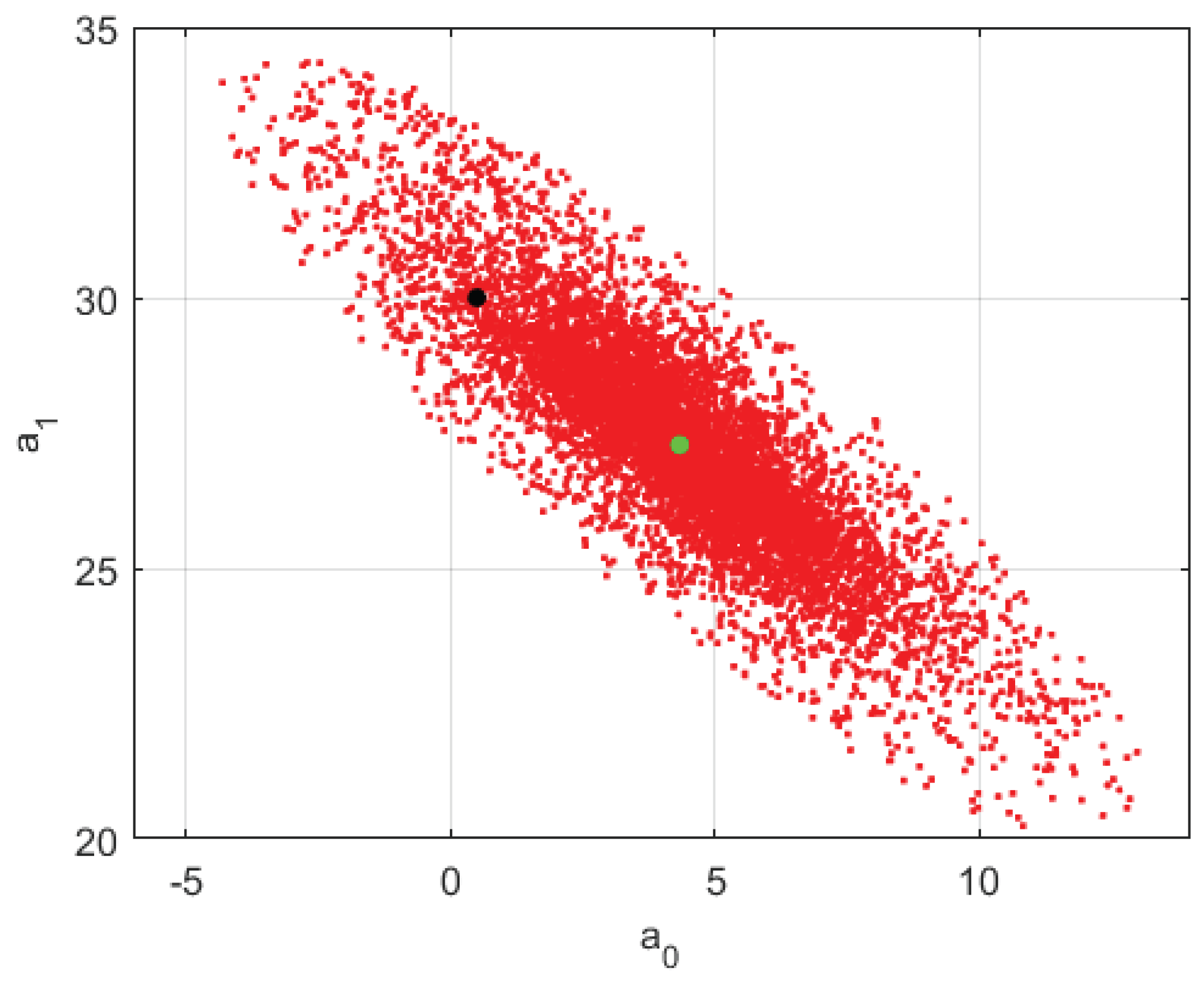
Figure 2.
Flowchart of the PSO-based inversion and uncertainty analysis for gravity anomaly detection.
Figure 2.
Flowchart of the PSO-based inversion and uncertainty analysis for gravity anomaly detection.
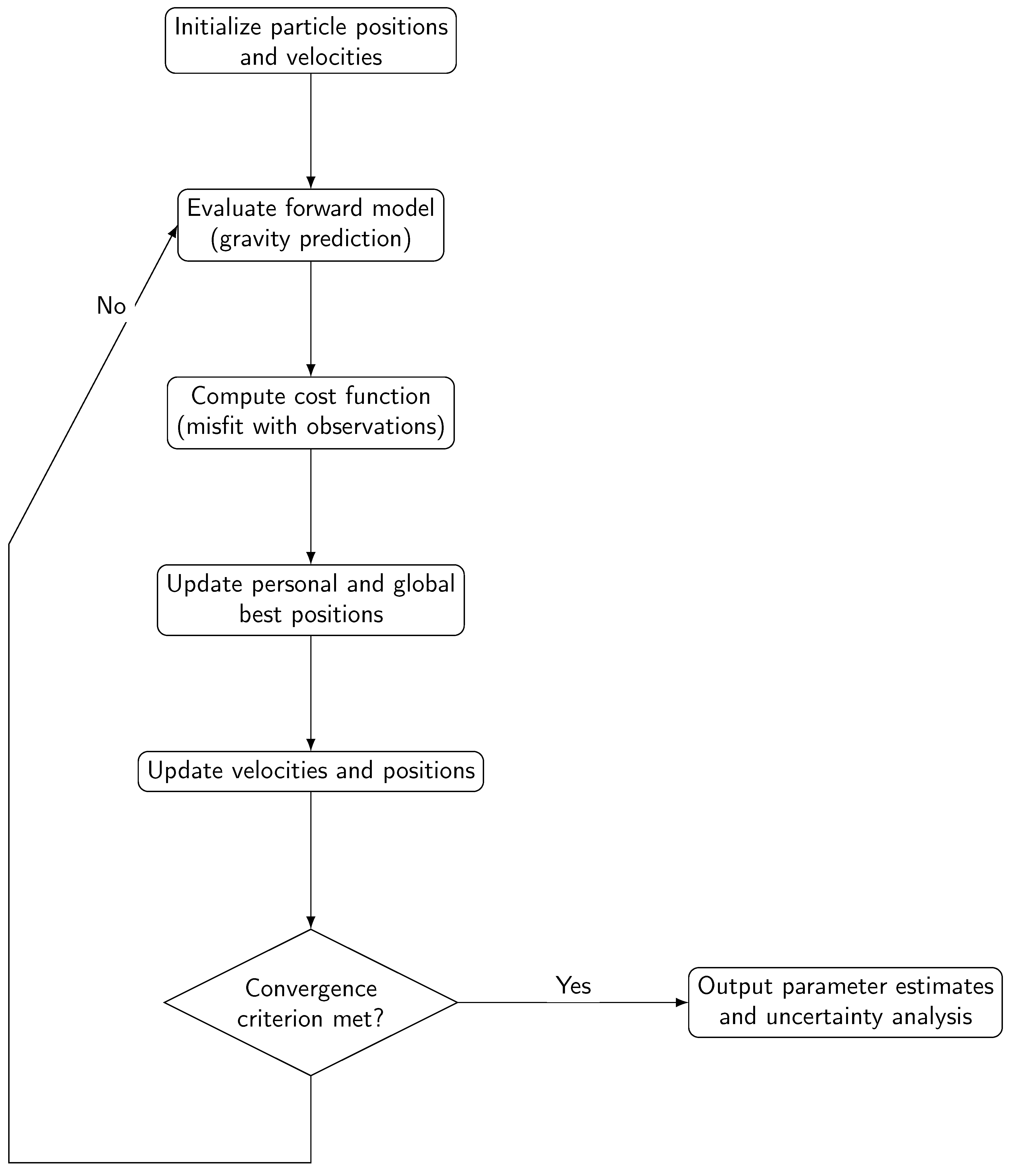
Figure 3.
Marginal histograms and pairwise correlation coefficients for the inverted parameters. Distributions are non-Gaussian and weakly correlated.
Figure 3.
Marginal histograms and pairwise correlation coefficients for the inverted parameters. Distributions are non-Gaussian and weakly correlated.
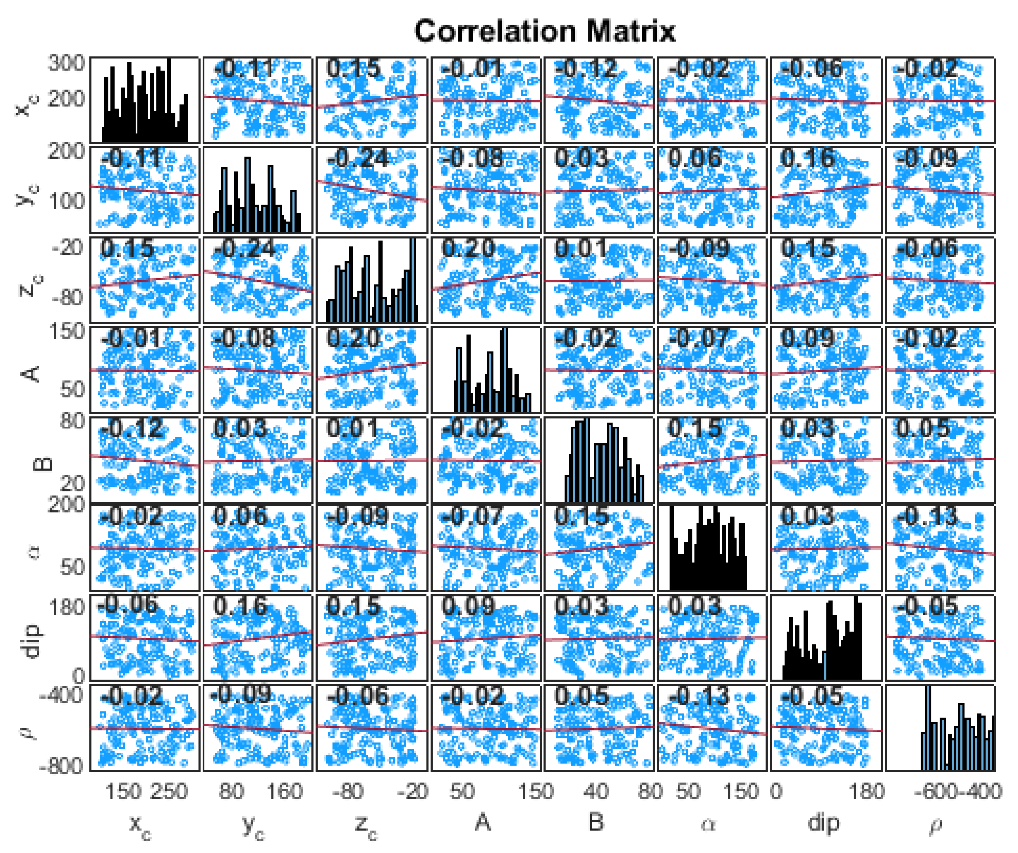
Figure 4.
One anomaly case. True and inverted ellipsoids (lowest misfit) in plan and front views. Good agreement in geometry and position is observed.
Figure 4.
One anomaly case. True and inverted ellipsoids (lowest misfit) in plan and front views. Good agreement in geometry and position is observed.
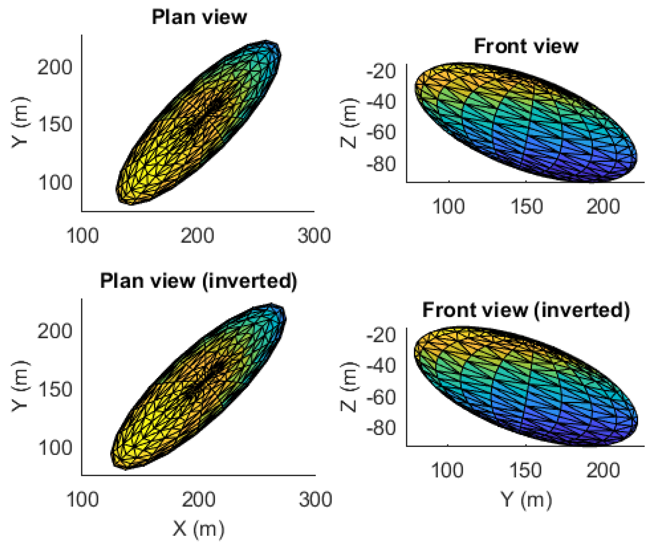
Figure 5.
One-anomaly case. PSO convergence curve showing the relative prediction error versus the number of iterations. Around iteration 120, the swarm converges to a region with a relative error of approximately .
Figure 5.
One-anomaly case. PSO convergence curve showing the relative prediction error versus the number of iterations. Around iteration 120, the swarm converges to a region with a relative error of approximately .
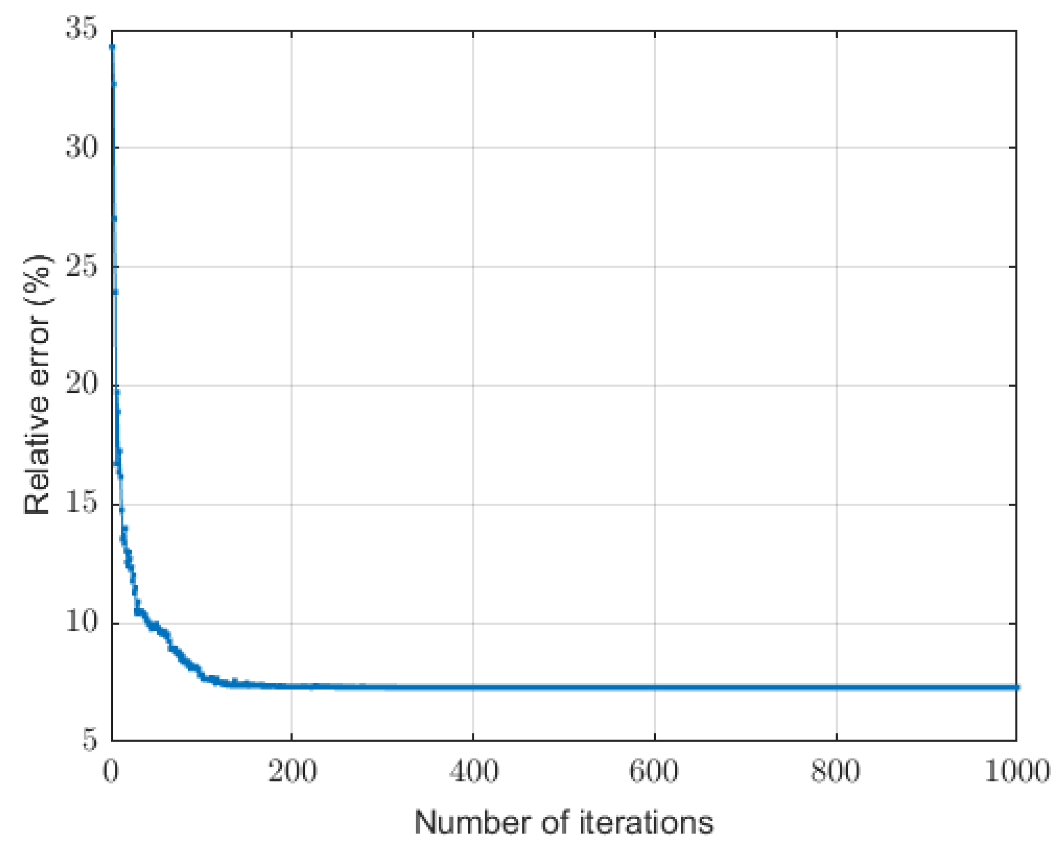
Figure 6.
One anomaly case. (a) Observed gravity anomaly (with noise) and (b) predicted anomaly from the best-fitting model.
Figure 6.
One anomaly case. (a) Observed gravity anomaly (with noise) and (b) predicted anomaly from the best-fitting model.
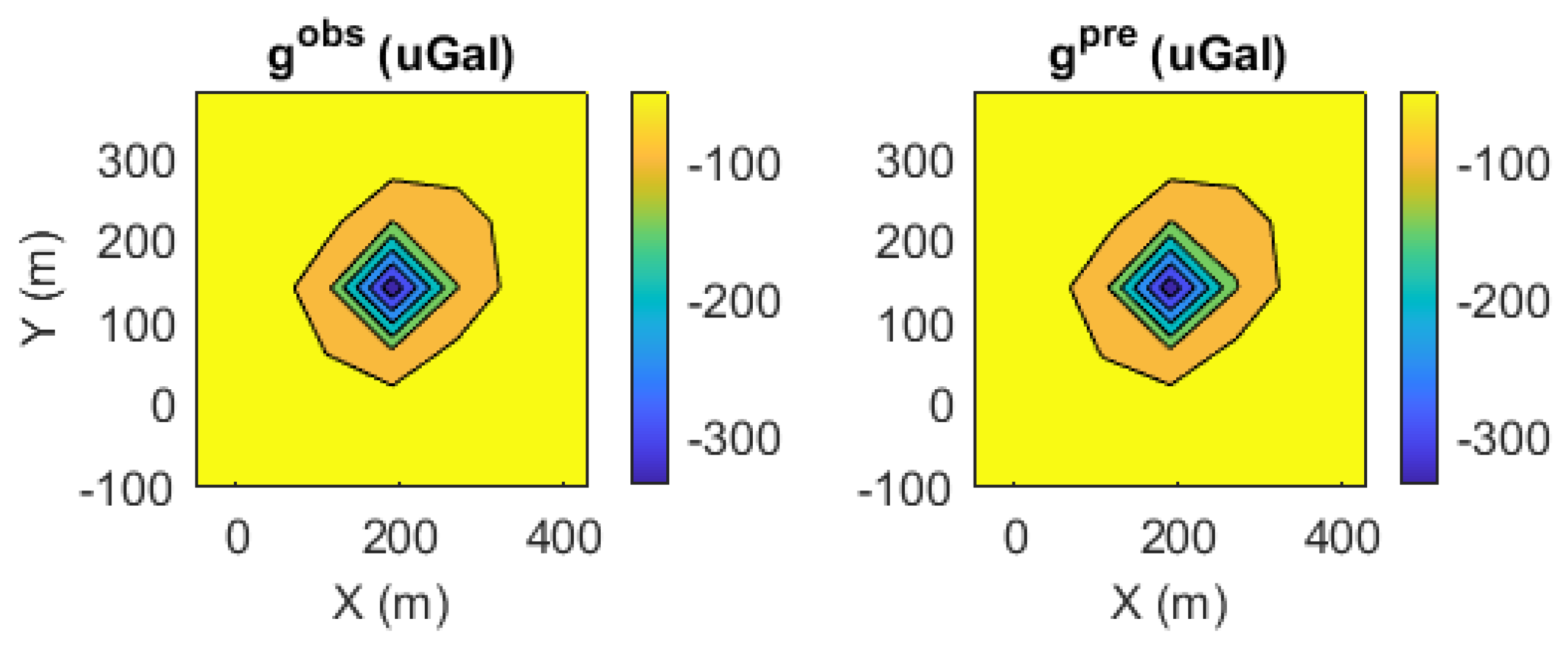
Figure 7.
Second example: true and best-fitting ellipsoids for the two-anomalies case (plan and front views).
Figure 7.
Second example: true and best-fitting ellipsoids for the two-anomalies case (plan and front views).
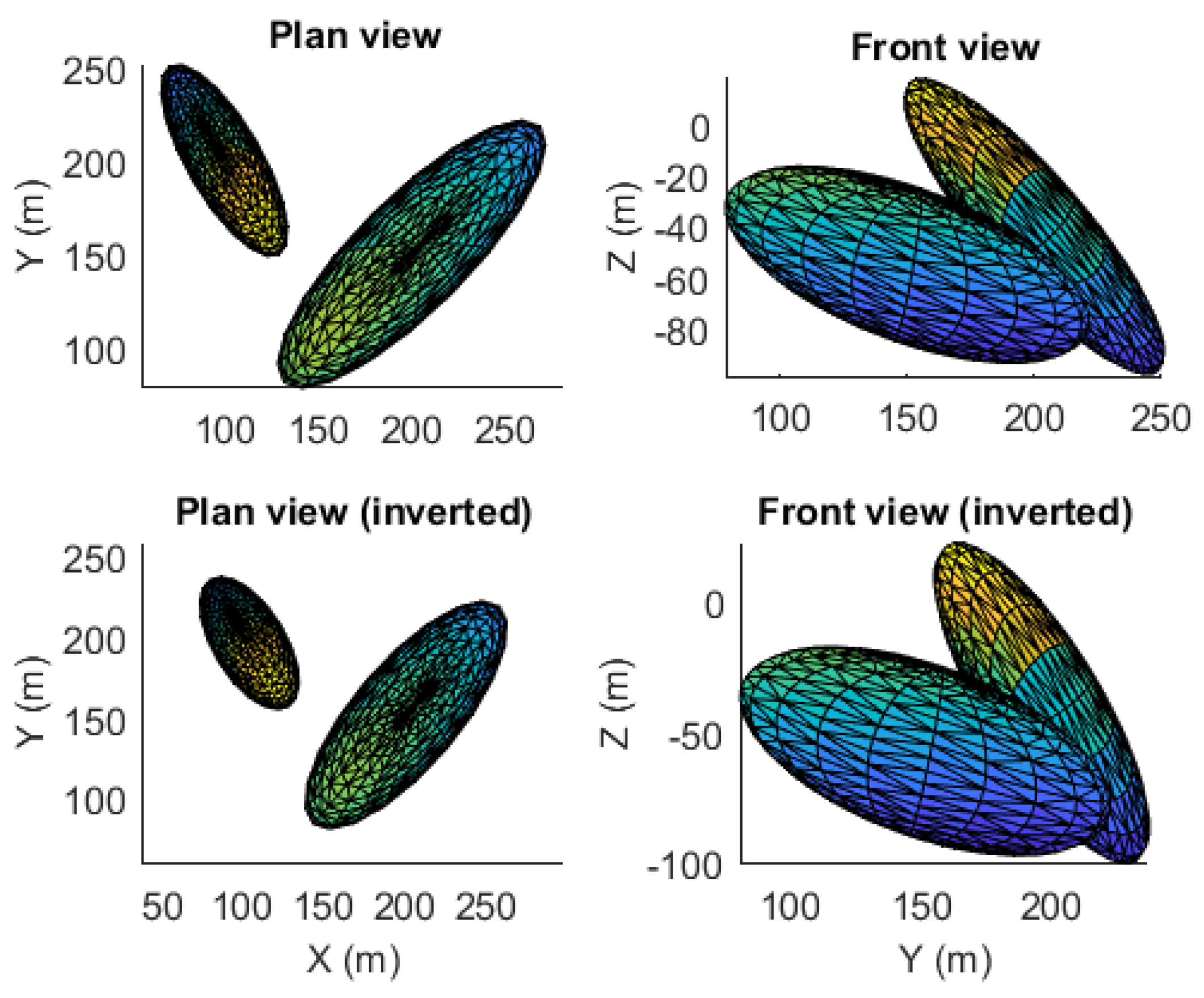
Figure 8.
Two-Anomaly Case: The PSO convergence curve illustrates the relative prediction error as a function of the iteration number. The curve exhibits a stepwise behavior, with the swarm converging to a region around iteration 225, where the relative error stabilizes at approximately .
Figure 8.
Two-Anomaly Case: The PSO convergence curve illustrates the relative prediction error as a function of the iteration number. The curve exhibits a stepwise behavior, with the swarm converging to a region around iteration 225, where the relative error stabilizes at approximately .
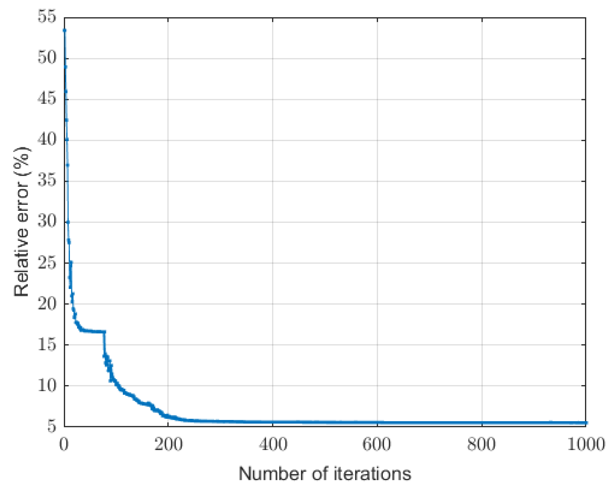
Figure 9.
Two anomalies case. (a) Observed (with noise) and (b) predicted gravity anomaly.
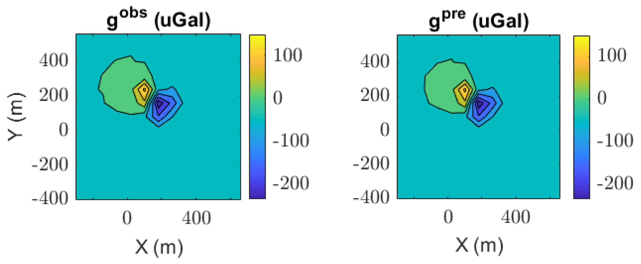
Figure 10.
Illustration of typical PSO behavior: (a) dispersion of the swarm and (b) proportion of particles remaining within the search boundaries over the course of iterations.
Figure 10.
Illustration of typical PSO behavior: (a) dispersion of the swarm and (b) proportion of particles remaining within the search boundaries over the course of iterations.
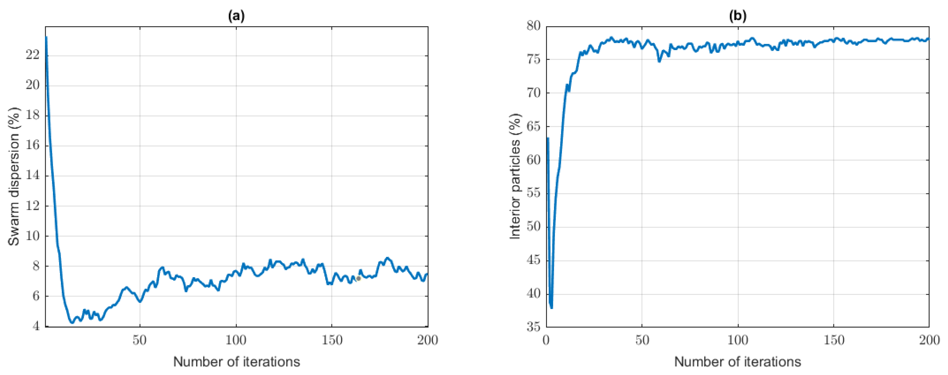
Figure 11.
(a) Total CPU time and (b) final relative error versus the number of swarm particles in the PSO algorithm.
Figure 11.
(a) Total CPU time and (b) final relative error versus the number of swarm particles in the PSO algorithm.
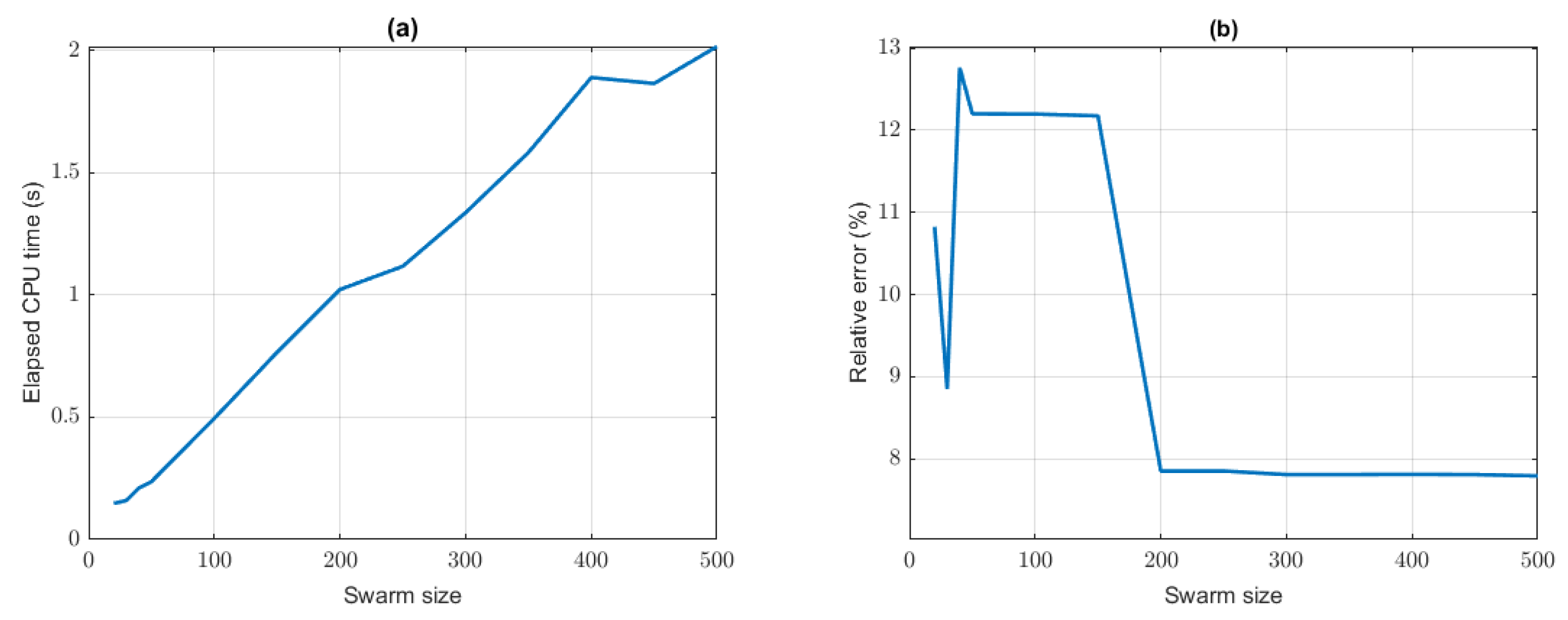
Figure 12.
Standard case. Water-filled karstic cavity: comparison between true and inverted ellipsoids in plan and front views.
Figure 12.
Standard case. Water-filled karstic cavity: comparison between true and inverted ellipsoids in plan and front views.
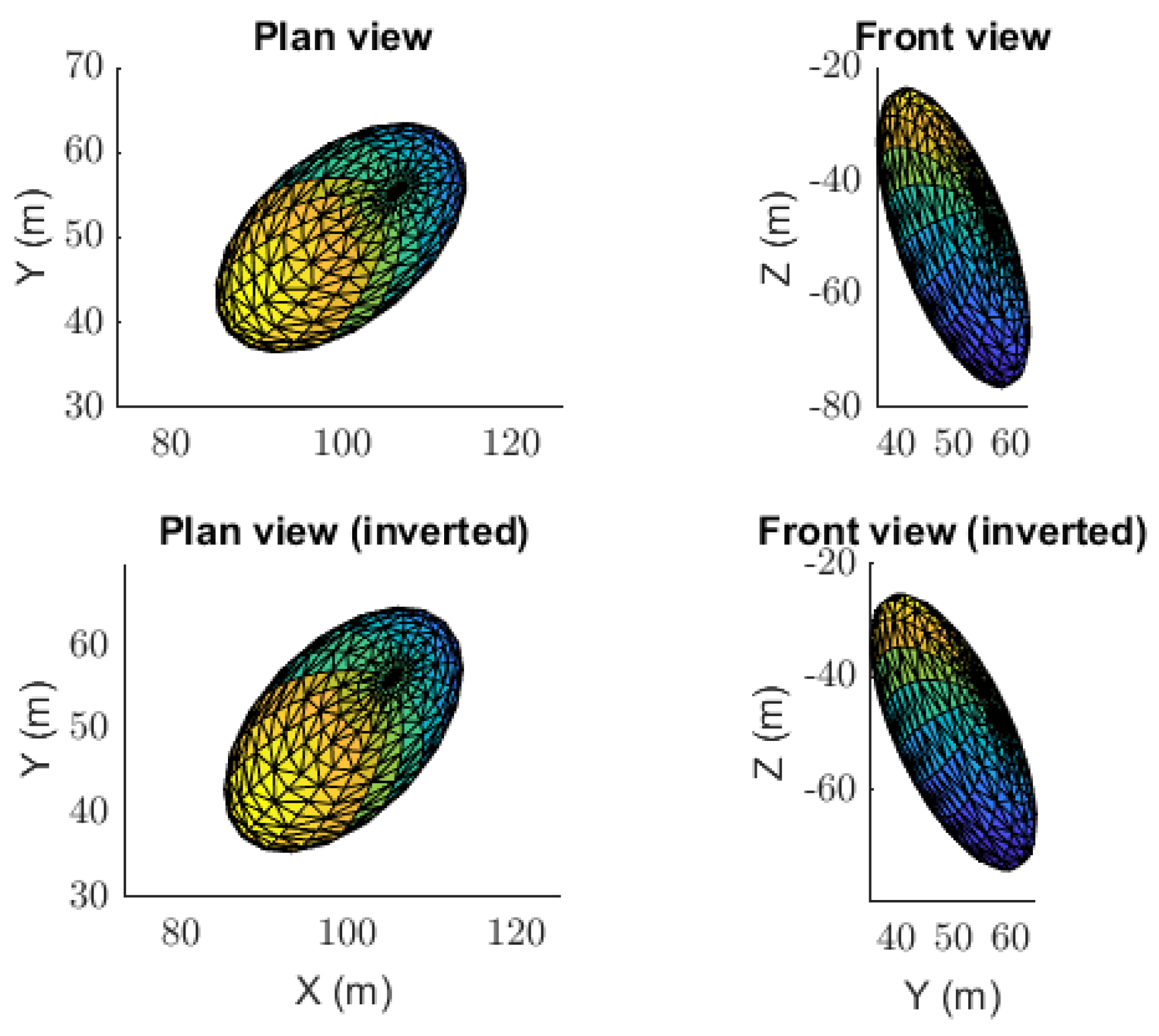
Figure 13.
Standard case. PSO convergence curve for the water-filled cavity inversion, showing relative misfit versus iteration number.
Figure 13.
Standard case. PSO convergence curve for the water-filled cavity inversion, showing relative misfit versus iteration number.
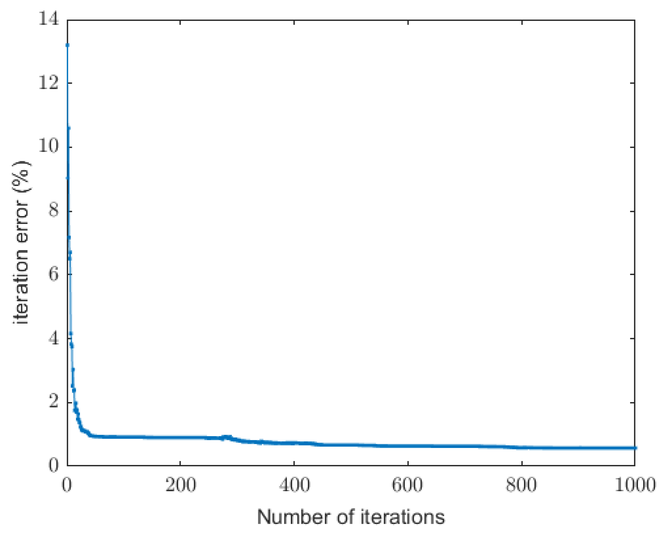
Figure 14.
Standard case. Gravity anomalies in the water-filled cavity model: (a) observed data and (b) predicted response.
Figure 14.
Standard case. Gravity anomalies in the water-filled cavity model: (a) observed data and (b) predicted response.

Figure 15.
Narrow case. Water-filled karstic cavity: comparison between true and inverted models in plan and front views.
Figure 15.
Narrow case. Water-filled karstic cavity: comparison between true and inverted models in plan and front views.
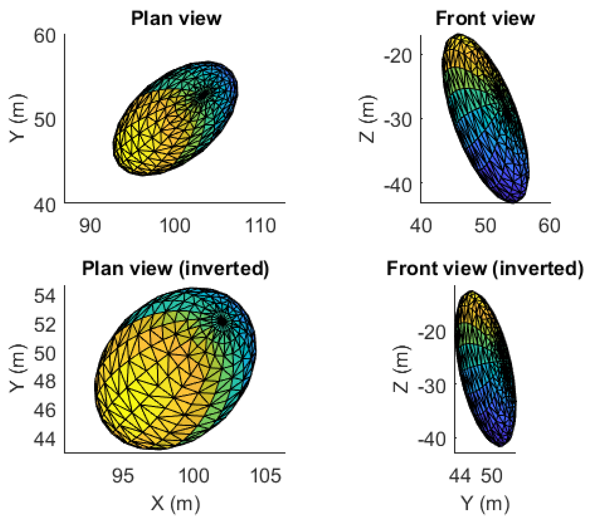
Figure 16.
Narrow case. Convergence curve for the inversion of a water-filled karstic cavity. Relative error versus iteration number.
Figure 16.
Narrow case. Convergence curve for the inversion of a water-filled karstic cavity. Relative error versus iteration number.
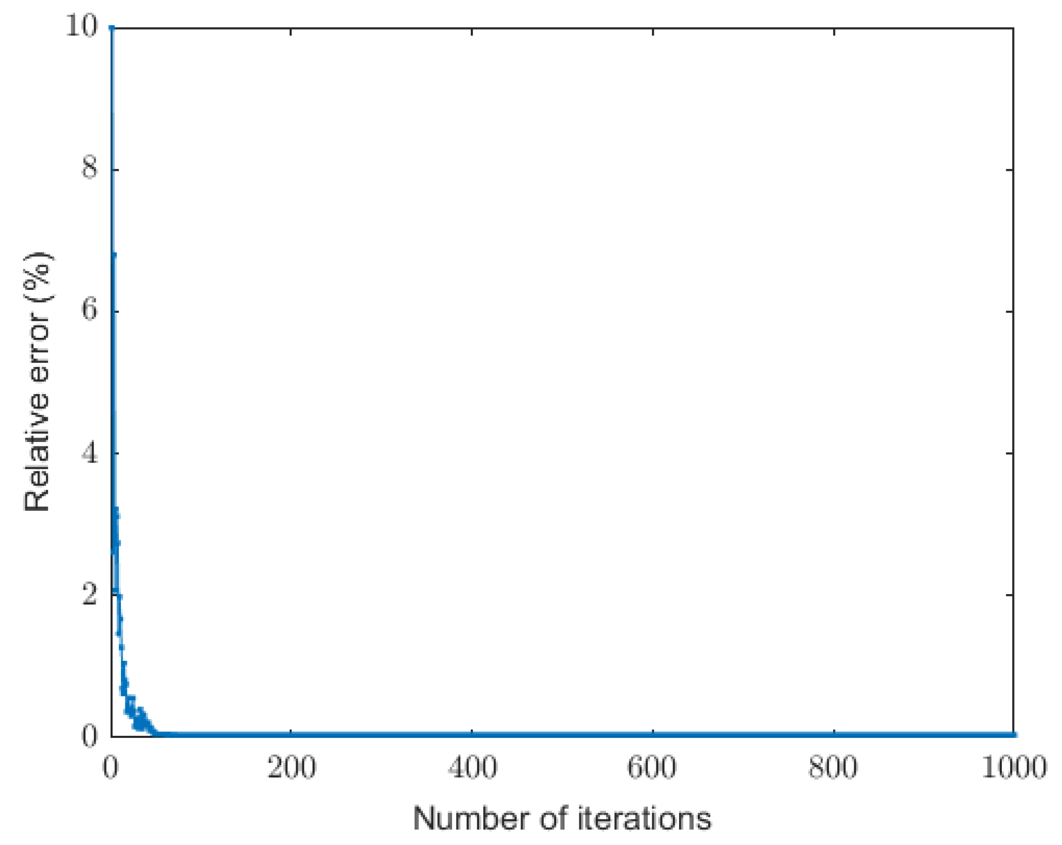
Figure 17.
Narrow karstic cavity filled with water. (a) Noisy observed gravity anomaly and (b) corresponding predicted anomaly from the inverted model.
Figure 17.
Narrow karstic cavity filled with water. (a) Noisy observed gravity anomaly and (b) corresponding predicted anomaly from the inverted model.
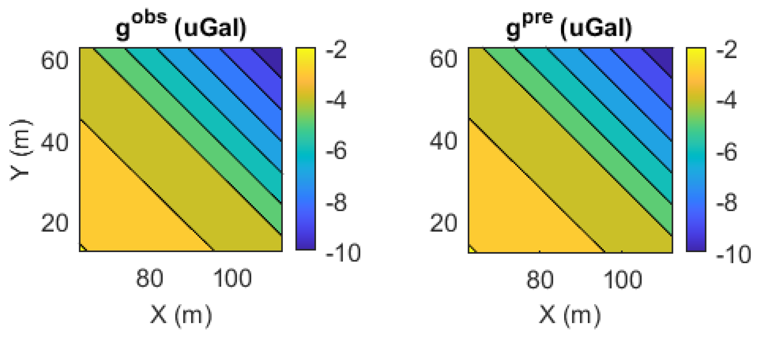

Table 1.
True model (TM), best-fitting model with the lowest prediction error (BM), and median of the models with less than prediction error (MedM). Also shown are the interquartile range (IQR), the normalized interquartile range (IQRn), and the minimum (Min) and maximum (Max) parameter values among the accepted models.
| A | B | |||||||
| TM | 200 | 150 | -55 | 100 | 30 | 45 | 165 | -600 |
| BM | 199.8 | 150.1 | -54.7 | 102.4 | 29.9 | 46.9 | 165.7 | -594.7 |
| MedM | 196.9 | 117.3 | -64.0 | 83.4 | 42.0 | 96.1 | 105.6 | -585.3 |
| IQR | 93.3 | 63.8 | 44.5 | 62.6 | 32.3 | 81.0 | 96.7 | 201.1 |
| IQRn | 0.47 | 0.54 | 0.69 | 0.75 | 0.77 | 0.84 | 0.92 | 0.34 |
| Min | 100 | 50 | -100 | 20 | 10 | 0 | 0 | -800 |
| Max | 300 | 200 | -20 | 150 | 80 | 180 | 180 | -400 |
Table 2.
Summary of 500 independent PSO inversions. Shown are: best-fitting model (BM), median (MedM), mean (MeanM), interquartile range (IQR), normalized interquartile range (IQRn), and coefficient of variation using standard deviation (cvs).
Table 2.
Summary of 500 independent PSO inversions. Shown are: best-fitting model (BM), median (MedM), mean (MeanM), interquartile range (IQR), normalized interquartile range (IQRn), and coefficient of variation using standard deviation (cvs).
| A | B | |||||||
| BM | 179.9 | 110.3 | -66.5 | 68.6 | 35.3 | 74.0 | 71.4 | -757.2 |
| MedM | 189.7 | 123.6 | -62.1 | 88.3 | 42.1 | 84.1 | 78.6 | -612.0 |
| MeanM | 197.7 | 124.8 | -60.8 | 89.1 | 43.9 | 89.4 | 86.0 | -610.9 |
| IQR | 97.8 | 72.0 | 36.1 | 66.2 | 28.1 | 80.5 | 74.2 | 201.5 |
| IQRn | 0.49 | 0.59 | 0.66 | 0.74 | 0.76 | 0.99 | 0.98 | 0.33 |
| cvs | 0.29 | 0.34 | 0.38 | 0.43 | 0.44 | 0.57 | 0.57 | 0.19 |
Table 3.
Ellipsoid 1: Inversion results compared with the true model (TM). Shown are: best-fitting model (BM), median of models with prediction error (MedM), interquartile range (IQR), normalized interquartile range (IQRn), and parameter bounds (Min, Max).
Table 3.
Ellipsoid 1: Inversion results compared with the true model (TM). Shown are: best-fitting model (BM), median of models with prediction error (MedM), interquartile range (IQR), normalized interquartile range (IQRn), and parameter bounds (Min, Max).
| Ellipsoid 1 | A | B | ||||||
| TM | 200 | 150 | -55 | 100 | 30 | 45 | 165 | -600 |
| BM | 201.1 | 151.4 | -57.2 | 91.7 | 32.6 | 40.5 | 164.3 | -564.0 |
| MedM | 201.2 | 113.3 | -57.5 | 88.7 | 41.8 | 79.5 | 84.0 | -571.7 |
| IQR | 106.4 | 81.4 | 39.7 | 65.6 | 36.2 | 73.2 | 77.5 | 199.4 |
| IQRn | 0.53 | 0.73 | 0.69 | 0.74 | 0.86 | 0.92 | 0.92 | 0.35 |
| Min | 100 | 50 | -100 | 20 | 10 | 0 | 0 | -800 |
| Max | 300 | 200 | -20 | 150 | 80 | 180 | 180 | -400 |
Table 4.
Ellipsoid 2: Same structure as Table 3. Includes TM, BM, MedM, IQR, IQRn, and parameter bounds within the accepted solution set.
Table 4.
Ellipsoid 2: Same structure as Table 3. Includes TM, BM, MedM, IQR, IQRn, and parameter bounds within the accepted solution set.
| Ellipsoid 2 | A | B | ||||||
| TM | 100 | 200 | -40 | 80 | 20 | 150 | 45 | 800 |
| BM | 104.1 | 195.9 | -38.8 | 73.5 | 22.4 | 148.6 | 54.7 | 798.5 |
| MedM | 110.8 | 195 | -48.0 | 52.7 | 25.2 | 92.6 | 95.2 | 799.1 |
| IQR | 73.0 | 89.6 | 47.5 | 43.2 | 16.1 | 96.0 | 85.9 | 198.2 |
| IQRn | 0.66 | 0.46 | 0.99 | 0.82 | 0.64 | 1.03 | 0.90 | 0.25 |
| Min | 30 | 100 | -90 | 20 | 5 | 0 | 0 | 600 |
| Max | 200 | 300 | -10 | 100 | 50 | 180 | 180 | 1000 |
Table 5.
Water-filled cavity (standard size): Best-fitting model (BM), median (MedM), mean (MeanM), interquartile range (IQR), normalized IQR (IQRn), and coefficient of variation using standard deviation (cvs). The density contrast is assumed known.
Table 5.
Water-filled cavity (standard size): Best-fitting model (BM), median (MedM), mean (MeanM), interquartile range (IQR), normalized IQR (IQRn), and coefficient of variation using standard deviation (cvs). The density contrast is assumed known.
| A | B | |||||||
| TM | 100 | 50 | -50 | 30 | 10 | 50 | 120 | -1400 |
| BM | 99.4 | 50 | -49.7 | 28.3 | 10.3 | 43.3 | 122.9 | -1400 |
| MedM | 99.0 | 42.7 | -50.2 | 32.7 | 12.7 | 66.4 | 109.5 | -1400 |
| MeanM | 98.6 | 44.1 | -50.5 | 34.0 | 12.5 | 80.0 | 100.4 | -1400 |
| IQR | 45.5 | 33.1 | 20.4 | 19.7 | 7.2 | 96.9 | 90.2 | 0 |
| IQRn | 0.46 | 0.77 | 0.41 | 0.60 | 0.57 | 1.46 | 0.82 | 0 |
| cvs | 0.28 | 0.45 | 0.23 | 0.40 | 0.33 | 0.68 | 0.51 | 0 |
| Min | 50 | 10 | -70 | 10 | 5 | 0 | 0 | -1400 |
| Max | 150 | 80 | -30 | 60 | 20 | 180 | 180 | -1400 |
Table 6.
Inversion results for a narrow water-filled cavity. Displayed statistics are as in Table 5: best-fitting model (BM), median of low-error models (MedM), interquartile range (IQR), normalized interquartile range (IQRn), coefficient of variation from standard deviation (cvs), and the search bounds (Min, Max). Tighter a priori bounds were used to improve detection accuracy in the narrow anomaly.
| A | B | |||||||
| TM | 100 | 50 | -30 | 15 | 5 | 50 | 120 | -1400 |
| BM | 98.7 | 48.8 | -27.1 | 15.2 | 4.9 | 44.5 | 106.6 | -1400 |
| MedM | 98.7 | 43.4 | -28.9 | 15 | 4.9 | 90.7 | 95.5 | -1400 |
| MeanM | 101.5 | 45 | -28.8 | 15 | 5 | 91.5 | 92.6 | -1400 |
| IQR | 44.9 | 34.4 | 3.6 | 2.0 | 1.8 | 90.0 | 90.5 | 0 |
| IQRn | 0.45 | 0.79 | 0.12 | 0.13 | 0.37 | 0.99 | 0.95 | 0 |
| cvs | 0.26 | 0.45 | 0.08 | 0.07 | 0.23 | 0.56 | 0.56 | 0 |
| Min | 50 | 10 | -35 | 10 | 2 | 0 | 0 | -1400 |
| Max | 150 | 80 | -25 | 20 | 10 | 180 | 180 | -1400 |
Disclaimer/Publisher’s Note: The statements, opinions and data contained in all publications are solely those of the individual author(s) and contributor(s) and not of MDPI and/or the editor(s). MDPI and/or the editor(s) disclaim responsibility for any injury to people or property resulting from any ideas, methods, instructions or products referred to in the content. |
© 2025 by the authors. Licensee MDPI, Basel, Switzerland. This article is an open access article distributed under the terms and conditions of the Creative Commons Attribution (CC BY) license (https://creativecommons.org/licenses/by/4.0/).
Copyright: This open access article is published under a Creative Commons CC BY 4.0 license, which permit the free download, distribution, and reuse, provided that the author and preprint are cited in any reuse.


