
Submitted:
19 October 2025
Posted:
20 October 2025
You are already at the latest version
Abstract
Developing a high–precision regional geoid model is a key element in moderniz-ing Kazakhstan’s vertical reference framework and ensuring consistent GNSS-based height determination. However, the mountainous terrain of southeastern Kazakhstan, characterized by strong topographic gradients and sparse terrestrial gravity coverage, poses significant modelling challenges. This study presents the first AI–enhanced hy-brid geoid model developed for the Almaty region, integrating classical gravimetric modelling with modern machine-learning simulation. The baseline solution was com-puted using the Least-Squares Modification of Stokes’ Formula with Additive correc-tions, combining digitized Soviet-era terrestrial gravity data, the global geopotential model XGM2019e_2159, and the FABDEM 30 m digital elevation model. Validation using GNSS/leveling benchmarks revealed a systematic bias of −0.08 m and an RMS of 0.10 m. To improve the fit between modelled and observed undulations, three ma-chine-learning regressors – Gaussian Process Regression (GPR), Support Vector Re-gression (SVR), and LSBoost—were applied to model the residual correction surface. Among them, the SVR model achieved the optimal balance between accuracy and generalization, reducing the test RMS to 0.032 m without overfitting. The resulting hybrid model, designated NALM2025, achieved centimeter-level consistency with GNSS/leveling data. The results demonstrate that integrating classical geoid computa-tion with AI–based residual modelling provides an efficient computational framework for high-precision geoid determination in complex mountainous environments.
Keywords:
modeling
; geoid model
; LSMSA
; Helmert transformation
; machine-learning regressors
; Gaussian Process Regression
; Support Vector Regression
; LSBoost
1. Introduction
The creation of a precise geoid model is one of the most important tasks of modern geodesy, as it forms the foundation for establishing a unified national height system. This is particularly relevant for countries with vast territories and complex topography. The Republic of Kazakhstan, the ninth largest country in the world by area, is characterized by pronounced elevation contrasts, ranging from the Caspian Lowland to the mountain ranges of the Tien Shan and Altai. Under such conditions, the use of global geopotential models (GGMs), such as EGM2008 or XGM2019e, provides only an averaged description of the gravity field and does not allow achieving high accuracy level required for engineering and geodetic applications. Therefore, a tailored and customized model is required for such terrains. Conventionally, geodetic data obtained using leveling techniques and the global navigation satellite system (GNSS) is used for geoid modelling. However, they do have some disadvantages: Field surveying is expensive especially in remote and difficult-to access areas, and there are very few GNSS stations and it is time consuming to level up after each leveling operation. Also, data gaps might result from processes [1,2].
The development of high precision model is one of the key tasks within the framework of ongoing national program on establishment of state coordinate and height system. This will enable the replacement of labor-intensive and expensive geometric leveling with GNSS technologies, where the orthometric height is determined as the difference between the ellipsoidal height and the geoid height. Such a transition will ensure a significant reduction in costs while maintaining high accuracy and efficiency of geodetic works.
Over the last two decades, significant progress has been made in developing refined gravimetric geoid determination methods. The Least-Squares Modification of Stokes’ Formula with Additive corrections (LSMSA, also known as the KTH method) has become a widely accepted framework for regional geoid modelling [3,4,5,6]. This method rigorously integrates heterogeneous data-gravity anomalies, DEM-derived terrain corrections, and GGMs-while accounting for truncation and spectral errors. However, residual discrepancies between gravimetric solutions and GNSS/leveling observations often remain due to datum inconsistencies, measurement noise, or local heterogeneities [7]. Traditionally, such residuals have been minimized using low-parameter Helmert transformations; yet, these approaches may overfit and cannot adequately represent complex local biases.
Recent advances in machine learning (ML) have opened new opportunities for geodetic modelling, offering flexible, data-driven alternatives for residual correction. Methods such as Gaussian Process Regression (GPR), Support Vector Regression (SVR), and ensemble learners (e.g., LSBoost) have demonstrated the ability to capture nonlinear relationships and provide robust predictive performance across geospatial domains [6,8,9,10,11]. Their application to geoid modelling remains relatively new, but early studies suggest that ML-based corrector surfaces can significantly improve hybrid geoid accuracy compared to conventional techniques [12,13,14].
In this study we aim to develop a high-resolution hybrid geoid model for the Almaty region of southeastern Kazakhstan using LSMSA method and machine learning. We integrate digitized terrestrial gravity data, the global model XGM2019e_2159, the FABDEM 30 m DEM, and a network of GNSS/leveling benchmarks. The geoid is first computed using the LSMSA method to obtain a physically consistent gravimetric baseline. Subsequently, residual corrections are modeled using both classical Helmert fitting and advanced machine-learning regressors (GPR, SVR, LSBoost), enabling a comparative assessment of accuracy, robustness, and generalization. The final outcome is a refined hybrid geoid surface (NALM2025), designed to support precise geodetic, engineering, and scientific applications in one of the most challenging regions of Kazakhstan.
2. Study Area
The study area lies between latitudes 42.5°- 44° N and longitudes 76°-77.5° E, covering the southeastern part of Kazakhstan, specifically the Almaty region (Figure 1). This area includes the Zailiyskiy Alatau Range, a prominent subrange of the northern Tien Shan Mountains. The region is characterized by highly variable topography, with elevations ranging from approximately 600 meters in the lowlands to over 5000 meters in the high mountain peaks. Such dramatic elevation differences within a relatively small spatial extent create a complex geophysical environment.
Geologically, the region is seismically active and dynamic due to ongoing tectonic convergence between the Eurasian and Indian plates. These tectonic activities result in pronounced crustal deformations and localized gravity anomalies. The combined effect of rugged terrain and active tectonics introduces significant challenges for geoid determination, especially when relying solely on global geopotential models (GGMs). The spatial variation of gravity and topographic masses in this region often exceeds the resolution and accuracy capabilities of global models, necessitating the application of regional hybrid geoid modelling techniques.
Furthermore, the Almaty region holds strategic importance for geodetic and surveying activities due to its urban expansion, infrastructure development, and the presence of numerous scientific institutions. Accurate geoid models are critical for precise height systems and geospatial applications in such a topographically and geophysically complex region. Therefore, this area serves as an ideal testbed for evaluating the performance of hybrid geoid modelling methods that integrate satellite-based models, terrestrial gravity data, and digital elevation models (DEMs).
3. Information Base, Required for Local Geoid Modelling
The hybrid geoid model in this study is constructed using four complementary datasets: terrestrial gravity measurements, a global geopotential model (GGM), a high-resolution digital elevation model (DEM), and GNSS/levelling points. In present study, the long-wavelength component of the gravity field is represented by the global gravity model XGM2019e_2159, since it is one of the most up-to-date combined models integrating satellite (GRACE, GOCE) and terrestrial gravity data[15]. Topographic information and terrain corrections are derived from the FABDEM 30 m dataset, offering improved representation of bare-earth elevations [16]. The primary sources of information, however, are the gravity data—compiled from digitized historical surveys, validated by modern ground measurements, and harmonized with global models—and the GNSS/levelling data, which serve both for AI-supported geoid correction and independent validation of the geoid.
3.1. Gravity Data
For this study, gravimetric data are sourced from Soviet-era gravity anomaly maps at a scale of 1:200,000. These maps provide extensive coverage and detailed gravity information across Kazakhstan, with over 90% of the national territory surveyed using gravimeters such as SN-3, GAK, and GR-2K. In priority regions, higher-resolution surveys (1:50,000 or finer) were conducted [15]. The maps are based on Bouguer anomaly reductions using densities of 2.30 g/cm³ and 2.67 g/cm³ and include associated metadata such as free-air anomalies, elevation values, and terrain corrections. Many of the 1:200,000-scale maps incorporated data from earlier surveys conducted at scales ranging from 1:25,000 to 1:50,000.
Historical gravity database was created by digitizing 14,061 gravity observation points from the following nomenclature sheets: L-43-XXVIII, L-43-XXIX, L-43-XXX, L-44-XXV, L-43-XXXIV, L-43-XXXV, L-44-XXXI, K-43-IV, K-43-V, K-43-VI, K-44-I, K-43-X, K-43-XI, K-43-XII, and K-44-VII. (Figure 2).
The digitization process includes scanning of original paper maps at a resolution of 600 dpi to preserve fine details, such as gravity isolines and control points. Subsequently, each scanned sheet was georeferenced to the WGS84 coordinate system using at least four control points, typically at coordinate grid intersections. The georeferencing was initially performed in the Pulkovo 1942 datum within the relevant Gauss–Krüger projection zone. Polynomial transformations (second or third order) were applied where necessary, and positional accuracy was maintained within 0.1-0.3 mm at the original map scale.
After georeferencing, vectorization of gravity anomaly contours and observation points was performed, and relevant attributes—such as Bouguer anomalies, terrain corrections, and elevations—were entered into structured attribute tables. Priority was given to maps with Bouguer reductions using 2.67 g/cm³ with terrain correction. Maps with 2.30 g/cm³ density reductions were used only in areas lacking higher-quality datasets.
A quality control procedure was implemented by generating a digital gravity anomaly surface using Kriging interpolation (250 × 250 m grid) and comparing it to the original raster images. Any discrepancies, often due to digitization errors, were corrected, and affected points were flagged in the database. Final data transformation from Gauss–Krüger coordinates to WGS84 was conducted using the transformation parameters Pulkovo_1942_To_WGS_1984_16. All digitized sheets were then merged into a unified spatial dataset.
To address data gaps in remote or mountainous areas lacking terrestrial surveys, global gravity data from the WGM2012 model (5′ × 5′ resolution) were integrated (Figure 3). These supplementary data enhanced the spatial continuity of the gravity field and were essential for accurate interpolation in regions where local measurements were unavailable.
To assess the reliability of the gravity data, a comparison was conducted with modern absolute gravity measurements from QazGRF (Kazakhstan Gravimetric Reference Frame) stations [17,18,19] (Figure 4). Bouguer anomaly values were interpolated from the gravity data and corrected to estimate absolute gravity, which was then compared against observed values.
The statistical evaluation shows a mean difference of 3.23 mGal and a standard deviation of 2.95 mGal, with over 90% of discrepancies within ±5 mGal. This indicates the absence of systematic bias and confirms the generally high quality of the gravity data. The dataset was subsequently converted into a free-air gravity anomaly grid, which served as the primary input for the LSMSA method in local geoid determination.
3.2. GNSS/Leveling Data
A hybrid geoid model was derived and validated from a combined dataset of GNSS observations and second- to third-order leveling benchmarks, integrated with first-order triangulation points (Figure 5).
The network covers both lowland and mountainous areas in southeastern Kazakhstan, which allows for accounting the diversity of topographic and geophysical conditions essential for precise geoid modelling. Normal heights, defined in the BHS-77 system, range from approximately 626 m to 1466 m and were compared with ellipsoidal heights derived from GNSS measurements, providing a basis for quantifying and minimizing systematic differences between the physical and geometric height systems. The GNSS surveys were conducted in static mode using dual-frequency GPS/GLONASS receivers, with observation sessions lasting no less than 24 hours to suppress atmospheric effects, including iono-spheric and tropospheric delays. The raw data were collected in RINEX format and processed with the GAMIT/GLOBK software package. The GAMIT module applied precise IGS orbits, atmospheric delay models, and multipath corrections based on double-difference carrier phase solutions, while GLOBK was used for network adjustment and integration into the global IGS reference frame through nearby permanent stations (BADG, LHAZ, URUM, NOVM). The full GNSS post-processing cycle is summarized in four main stages: (i) synchronization of data to a single time scale, (ii) elimination of atmospheric distortions, (iii) construction of baseline vectors between observation points, and (iv) least squares adjustment of coordinates to minimize random errors (Figure 6).
The quality of the adjusted solution was assessed using weighted root mean square (WRMS) values for the east, north, and vertical components, which in most cases were below 0.050 m, with the most stable stations, such as KOTU and KURS, achieving WRMS values as low as 0.004 m. Although some sites initially exhibited higher RMS values due to multipath effects, the final adjusted coordinates remained well within accepted geodetic precision.
4. Methods of the Local Geoid Modelling
The proposed methodology integrates the classical Least-Squares Modification of Stokes’ Formula with Additive corrections (LSMSA, also known as the KTH method) and advanced machine learning techniques to improve the accuracy of local geoid determination. The workflow is divided into three main stages (Figure 7).
The first stage of our workflow follows the classical LSMSA method [20] This approach provides a rigorous theoretical framework to integrate heterogeneous datasets — terrestrial gravity anomalies, global geopotential models (GGMs), digital elevation models, and GNSS/leveling observations — into a single regional geoid model.
The LSMSA method optimizes modification parameters of the Stokes kernel in a least-squares sense, thereby minimizing the mean square error of the derived geoid heights[17]. It accounts for:
- -
- truncation and spectral errors of gravity anomalies;
- -
- regularization of the poorly conditioned system for high-degree harmonics;
- -
- additive corrections for topography, atmosphere, ellipsoidal effects, and downward continuation.
The output is a gravimetric geoid model , which serves as the baseline solution for further refinement.
In the second stage, GNSS/leveling observations are preprocessed to geoid undulations compatible with the gravimetric baseline. Kazakhstan’s national height system is realized in normal heights—we first form height anomalies ζ and convert them to geoid undulations via the Moritz [21] geoid–quasigeoid separation formula, ensuring strict commensurability with the gravimetric geoid and an unbiased assessment of GNSS/Leveling results.
The resulting values are then split into training (70%) and test (30%) subsets for subsequent Helmert and AI comparisons.
The third stage consists of building a data-driven corrector surface from the pointwise residuals between GNSS/leveling undulations and the gravimetric baseline, and then superimposing this field on the LSMSA surface to obtain the final hybrid geoid. Traditionally, this is achieved with a 3-, 5- ,7-parameters Helmert transformation, which aligns the two datasets by modelling shifts, rotations, and scale distortions. However, Helmert fitting can introduce systematic errors when datasets use different vertical datums or contain topographic inconsistencies. To improve the flexibility and accuracy of residual modelling, we propose the use of AI-based regression methods to approximate the difference between GNSS/leveling values and the gravimetric LSMSA model.
Specifically, letdenote the feature vector composed of standard geodetic latitude and longitude (in decimal degrees) and the gravimetric baseline undulation interpolated at the point location. For each control point, we form the pointwise residual
and learn a data-driven regressor such that . The final hybrid geoid is then obtained by superimposition,
To approximate over the study area while preserving smooth, geophysically plausible behavior, we evaluate three complementary regression families: Gaussian Process Regression (GPR), Random Forest (RF), and Support Vector Regression (SVR). These methods are trained on 70% of the GNSS/leveling dataset and validated on the remaining 30%, ensuring reliable generalization.
GPR was implemented using an Automatic Relevance Determination Squared Exponential (ARD) kernel (GPR, ARD kernel). We place a Gaussian process prior on the latent field with i.i.d. Gaussian observation noise,
An automatic relevance determination (ARD) kernel is used so that the model learns separate length-scales for φ, λ, and NLSMSA. In practice we adopt a Matérn 3/2 covariance (with fallbacks to Matérn 5/2 or squared-exponential when required). Writing
The kernel read:
Given training inputs X and targets y, the posterior predictor at x* has mean and variance
with hyperparameters fitted by maximizing the log marginal likelihood. Using φ and λ as standard degrees is handled by ARD and z-standardization, which absorb scale differences between the angular and metric features.
Support Vector Regression (SVR, RBF kernel)
SVR seeks a function with small RKHS norm while keeping residuals within an ε -insensitive tube:
By the representer theorem,
with an RBF kernel . The hyperparameters C, ε, and σ (KernelScale) govern smoothness and robustness. As with GPR, inputs (φ,λ,NLSMSA) are kept in their standard units and standardized prior to training.
Least-Squares Boosting (LSBoost)
We fit an additive ensemble of regression trees by steepest descent on the squared loss. Starting from
we iterate for m=1,…,M:
with learning rate . Regularization is controlled by (M,ν) and tree complexity (e.g., minimum leaf size). This yields a flexible, piecewise-smooth approximation of ΔN(φ,λ,NLSMSA) that complements the smooth, kernel-based GPR/SVR models.
To assess the effectiveness of the proposed approach, we perform a comparative analysis of Helmert 7-parameter fitting versus AI-based regression fitting (GPR, RF, SVR).
The comparison is carried out on the 30% evaluation dataset using RMSE, MAE, correlation coefficients, and residual distribution statistics. The model achieving the best generalization performance and stability was selected as the final regression method for constructing the hybrid geoid model for the Almaty region.
5. Results and Discussion
5.1. Classical Geoid Modelling by LSMSA Method
Geoid model calculations included the use of XGM2019 spherical harmonic coefficients to powers of 120, 200, 300, 400, 500, 630, 760, with a combination of ground gravity data error variance C (0) - 0.5, 1, 3, 6, 9, 16 mGal2. The results are presented in Table 1, Figure 8.
The initial parameters for calculating the modification parameters were:
- Degree of modification L=M= 300;
- Variance of errors in ground gravity data C (0) =1 m Gal 2;
- The size of the integration coverage is Ѱ= 1o.
In the computational scheme of the LSMSA method for determining the geoid, the surface gravity anomalies and the GGM are used to determine Napp (Figure 9)., and then necessary corrections are added (Figure 10, Table 2).
Figure 11 shows the result of calculating the geoid heights for the study area using the method “Least Squares Modification of Stokes formula with additional corrections (LSMSA)”.
The calculated geoid heights for Almaty region using the LSMSA method vary in the range from -46.485 m to -37.644 m, the average value is -42.577 m, and the standard deviation is 2.873 m.
5.2. Corrector Surface by AI
We evaluated residuals between observed geoid undulations and the grid interpolated to 40 control points (train = 28, test = 12). Table 3 summarizes distributional statistics for the baseline (“Before”) and for four fitted models (“After”).
Table 4 presents the residual error statistics of geoid correction for the entire dataset (ALL), the training subset (TRAIN), and the validation subset (TEST).
In the baseline solution, the residuals exhibit a systematic negative bias (Mean ≈ –0.08 m) with an RMS of 0.097 m, indicating the presence of unmodeled systematic errors. Both training and test subsets show similar bias levels, confirming that the discrepancy is not random but systematic.
Application of the Helmert transformation reduces the training errors significantly (RMS = 0.031 m); however, the test subset deteriorates markedly (RMS = 0.248 m), revealing strong overfitting and poor generalization. Although effective in aligning datasets under controlled conditions, the method fails to provide stable corrections across independent data.
In contrast, the Gaussian Process Regression (GPR, ARD-SE kernel) achieves nearly unbiased residuals (Mean = –0.003 m) with the lowest RMS over the full dataset (0.025 m). The test subset maintains relatively high accuracy (RMS = 0.045 m), demonstrating superior generalization. The Support Vector Regression (SVR, RBF kernel) also provides stable results with low RMS values (0.039 m overall; 0.032 m on test), though slightly less accurate than GPR.
The LSBoost ensemble method yields the smallest overall RMS (0.022 m) and near-zero bias. While the training errors approach zero (RMS = 0.005 m), the test subset retains acceptable accuracy (RMS = 0.040 m), similar to GPR.
5.3. Hybrid Geoid (LSMSA + AI)
Given its superior held-out performance and balanced residual distribution, SVR (RBF) was selected for the final hybrid grid
The resulting grid, computed at 2′ × 2′ resolution, preserves the long-wavelength physical consistency of LSMSA while effectively removing local biases.
Residual statistics confirm a marked improvement that, the initial RMS of ~0.10 m was reduced to ~0.03–0.04 m, and the systematic offset (≈−0.08 m) was eliminated. Figure 12 illustrates the shift from a negatively biased distribution (before correction) to a centered and compact one after SVR-based adjustment.
6. Conclusions
This study successfully developed and evaluated a high-resolution hybrid geoid model for the Almaty region of southeastern Kazakhstan, one of the most topographically and geophysically complex areas in Central Asia. The work integrated digitized Soviet-era gravity data, the global geopotential model XGM2019e_2159, high-resolution DEMs, and GNSS/leveling benchmarks within the framework of the Least-Squares Modification of Stokes’ Formula with Additive corrections (LSMSA).
The baseline gravimetric solution demonstrated the ability of the LSMSA method to capture the long- and medium-wavelength features of the gravity field; however, systematic residuals of approximately –0.08 m remained when compared against GNSS/leveling observations. Classical Helmert transformation reduced these discrepancies in the training dataset but introduced instability and overfitting in the independent validation subset, confirming its limited suitability for robust hybrid modelling.
By contrast, machine-learning approaches provided substantial improvements. Gaussian Process Regression (GPR) and LSBoost yielded nearly unbiased residuals with RMS values in the range of 0.022–0.045 m, while Support Vector Regression (SVR, RBF kernel) offered a balance of accuracy and stability across training and test subsets. The final hybrid model, constructed using LSMSA combined with AI-based regression correction, achieved centimetre-level consistency with GNSS/leveling data and eliminated the systematic bias present in the baseline solution.
These results highlight two key conclusions. First, high-quality hybrid geoid models can be developed for regions with challenging topography by combining legacy gravimetric surveys with modern global and satellite-based datasets. Second, machine-learning regressors outperform classical parametric adjustments in modelling local residuals, offering a flexible and generalizable framework for future geoid determination efforts in Kazakhstan and comparable mountainous environments.
Future work will focus on expanding the methodology to a national scale, integrating additional GNSS/leveling networks.
Author Contributions
Conceptualization, A.U. and D.S.; methodology, A.U., D.S.; software, D.S., M.K.; validation, A.U., M.K., N.Z.; formal analysis, A.U.; investigation, A.U., D.S.; resources, A.U., S.N., data curation, M.K., N.Z.; writing-original draft preparation, A.U., D.S.; writing-review and editing, A.U., D.S..; visualization, M.K., N.Z.; supervision, A.U., D.S.; project administration, S.N. A.U.; funding acquisition, S.N. All authors have read and agreed to the published version of the manuscript
Funding
This research was funded by the Committee of Science of the Ministry of Science and Higher Education of the Republic of Kazakhstan (Grant No. BR21882366).
Data Availability Statement
Data are contained within this article
Acknowledgments
We are grateful to all the authors of the articles that were discussed in this review.
Conflicts of Interest
The authors declare no conflicts of interest
References
- M. A. Elshewy, P. Trung Thanh, A. M. Elsheshtawy, M. Refaat, and M. Freeshah, “A novel approach for optimizing regional geoid modeling over rugged terrains based on global geopotential models and artificial intelligence algorithms,” The Egyptian Journal of Remote Sensing and Space Sciences, vol. 27, no. 4, pp. 656–668, Dec. 2024. [CrossRef]
- F. Chen, X. Zhang, F. Guo, J. Zheng, Y. Nan, and M. Freeshah, “TDS-1 GNSS reflectometry wind geophysical model function response to GPS block types,” Taylor & FrancisF Chen, X Zhang, F Guo, J Zheng, Y Nan, M FreeshahGeo-Spatial Information Science, 2022•Taylor & Francis, vol. 25, no. 2, pp. 312–324, 2022. [CrossRef]
- R. A. Abbak and A. Ustun, “A software package for computing a regional gravimetric geoid model by the KTH method,” SpringerRA Abbak, A UstunEarth science informatics, 2015•Springer, vol. 8, no. 1, pp. 255–265, Mar. 2015. [CrossRef]
- M. S. Işık, B. Erol, S. Erol, and F. F. Sakil, “High-resolution geoid modeling using least squares modification of Stokes and Hotine formulas in Colorado,” J Geod, vol. 95, no. 5, May 2021. [CrossRef]
- H. Yildiz, R. Forsberg, J. Ågren, C. Tscherning, and L. Sjöberg, “Comparison of remove-compute-restore and least squares modification of Stokes’ formula techniques to quasi-geoid determination over the Auvergne test area,” Journal of Geodetic Science, vol. 2, no. 1, pp. 53–64, Jan. 2012. [CrossRef]
- R. A. Abbak, L. E. Sjöberg, A. Ellmann, and A. Ustun, “A precise gravimetric geoid model in a mountainous area with scarce gravity data: A case study in central Turkey,” Studia Geophysica et Geodaetica, vol. 56, no. 4, pp. 909–927, Oct. 2012. [CrossRef]
- Abdalla, S. M.-C. journal of earth sciences, and undefined 2015, “Implementation of a rigorous least-squares modification of Stokes’ formula to compute a gravimetric geoid model over Saudi Arabia (SAGEO13),” cdnsciencepub.comA Abdalla, S MogrenCanadian journal of earth sciences, 2015•cdnsciencepub.com, vol. 52, no. 10, pp. 823–832, Jun. 2015. [CrossRef]
- Abdalla and, D. Fairhead, “A new gravimetric geoid model for Sudan using the KTH method,” Journal of African Earth Sciences, vol. 60, no. 4, pp. 213–221, Jun. 2011. [CrossRef]
- R. A. Abbak, B. Erol, and A. Ustun, “Comparison of the KTH and remove-compute-restore techniques to geoid modelling in a mountainous area,” Comput Geosci, vol. 48, pp. 31–40, Nov. 2012. [CrossRef]
- P. Ulotu, “Geoid model of Tanzania from sparse and varying gravity data density by the KTH method,” (Doctoral dissertation, KTH), 2009.
- O. Karaca, B. Erol, and S. Erol, “Assessments of Gravity Data Gridding Using Various Interpolation Approaches for High-Resolution Geoid Computations,” Geosciences (Switzerland), vol. 14, no. 3, Mar. 2024. [CrossRef]
- F. Heeto Abdulrahman, “Determination of the local geoid model in Duhok Region, University of Duhok Campus as a Case study,” Ain Shams Engineering Journal, vol. 12, no. 2, pp. 1293–1304, Jun. 2021. [CrossRef]
- Sharafeldin Mohamed Osman et al., “Least Square Modification of Stokes Formulae with Additive Corrections Estimator for Klang Valley Geoid Modeling,” iopscience.iop.orgTK Ming, ZM Amin, AHM DinIOP Conference Series: Earth and Environmental Science, 2021•iopscience.iop.org, vol. 8, no. February 2018, pp. 68–74, 2017. [CrossRef]
- M. F. Pa’suya et al., “Hybrid geoid model over peninsular Malaysia (PMHG2020) using two approaches,” Studia Geophysica et Geodaetica, vol. 66, no. 3–4, pp. 98–123, Oct. 2022. [CrossRef]
- R. A. Sermiagin et al., “A historical overview of gravimetric surveys in Kazakhstan,” Geodesy and Cartography, vol. 1012, no. 10, pp. 53–64, Nov. 2024. [CrossRef]
- P. Zingerle, R. Pail, T. Gruber, and X. Oikonomidou, “The combined global gravity field model XGM2019e,” J Geod, vol. 94, no. 7, pp. 1–12, Jul. 2020. [CrossRef]
- L. E. Sjöberg and M. Bagherbandi, “Corrections in Geoid Determination. In Gravity Inversion and Integration: Theory and Applications in Geodesy and Geophysics,” Cham: Springer International Publishing, pp. 149–180, 2017.
- D. Tazhedinov, A. Islyamova, and M. Merkulov, “Technical Report on the mathematical processing (adjustment) of the stations of the 425 State Fundamental Gravimetric Network. Project code: K.04.00086,” Astana, (in Russian). 427 25., 2024.
- D. Tazhedinov, A. Islyamova, and M. Merkulov, “Technical Report on the results of the mathematical processing (adjustment) of 428 the stations of the State First-Order Gravimetric Network. Project code: K.04.00087.,” 2024, RSE National Centre of 429 Geodesy and Spatial Information.ermiagin, R. Dataset from Processing the 2023–2024 Campaigns to Establish Kazakhstan’s Gravity Reference Frame (QazGRF24), 431 2025 Astana. [CrossRef]
- L. S.-J. of geodesy and undefined 2003, “A general model for modifying Stokes’ formula and its least-squares solution,” SpringerLE SjöbergJournal of geodesy, 2003•Springer, vol. 77, no. 7–8, pp. 459–464, Oct. 2003. [CrossRef]
- H. Moritz, “Geodetic reference system 1980,” Bulletin Géodésique, vol. 66, no. 2, pp. 187–192, 1992. [CrossRef]
Figure 1.
Location and topography of the study area.
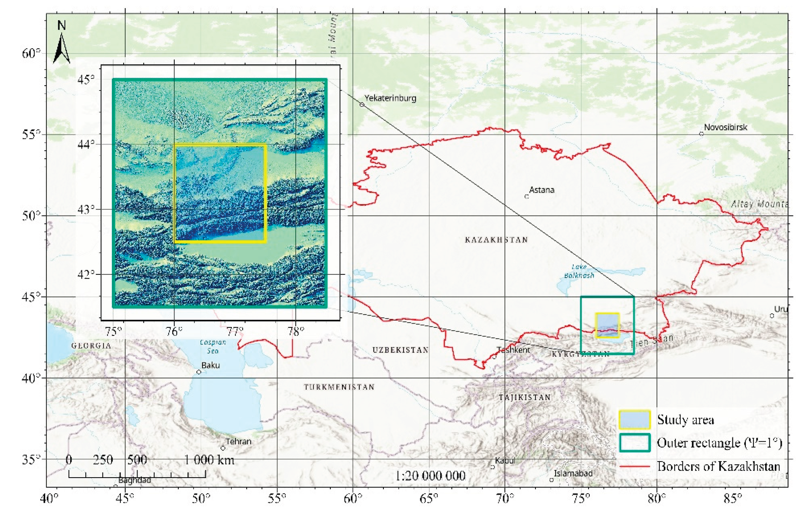
Figure 2.
Cartogram of digitized gravimetric maps at a scale of 1:200,000 for the study area.
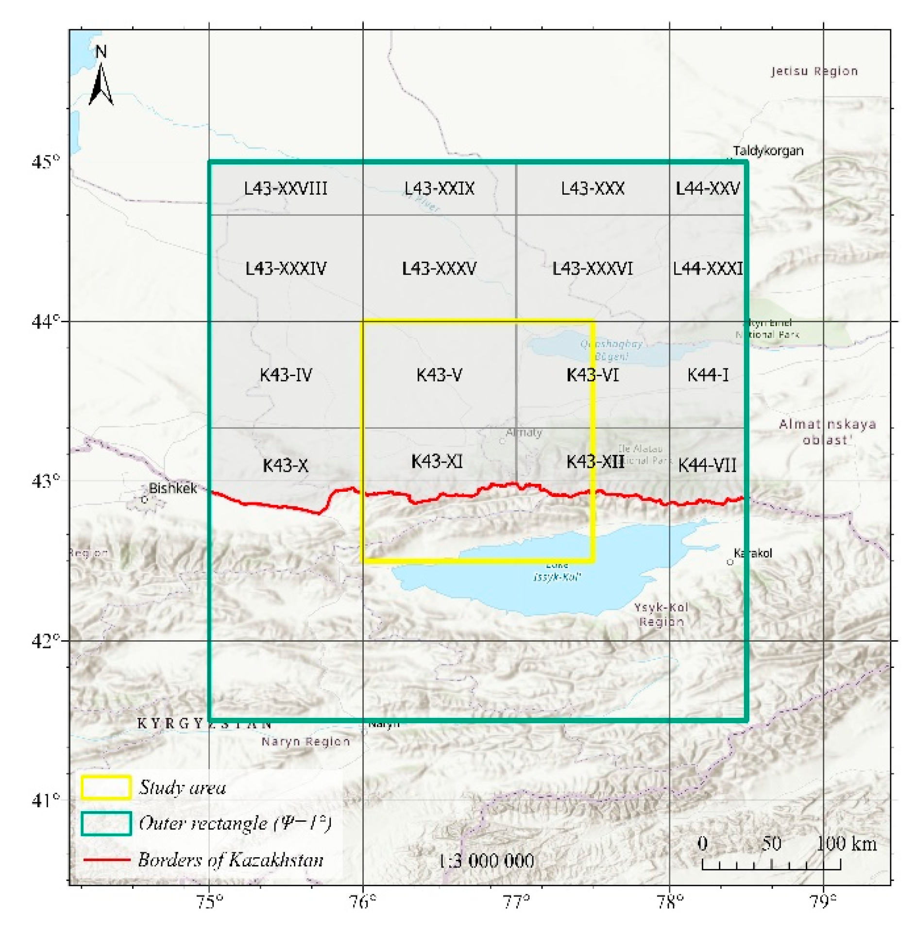
Figure 3.
Integration of ground-based gravity data with the global WGM2012 model.
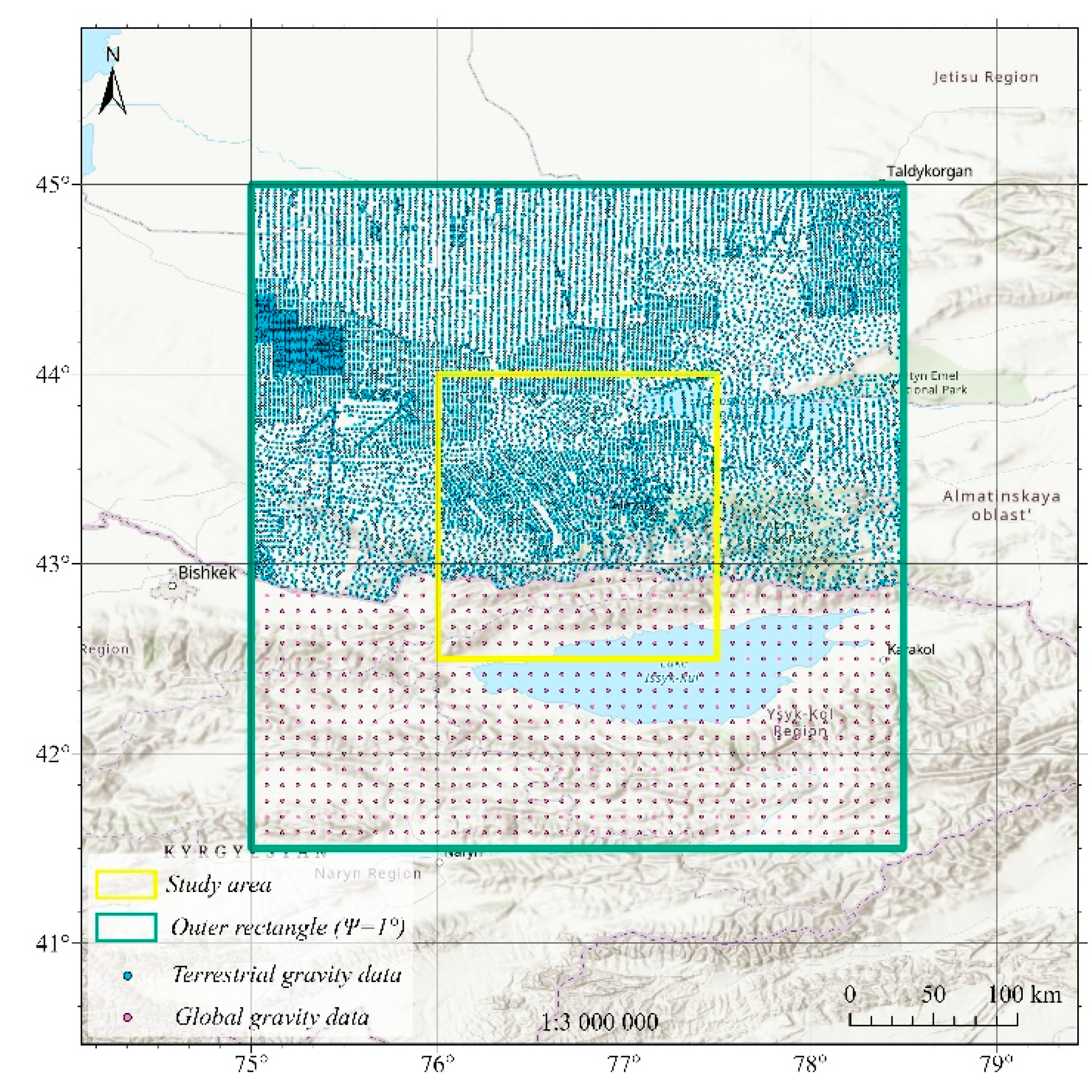
Figure 4.
Spatial distribution of QazGRF stations and Bouguer gravity anomalies over the study area.
Figure 4.
Spatial distribution of QazGRF stations and Bouguer gravity anomalies over the study area.
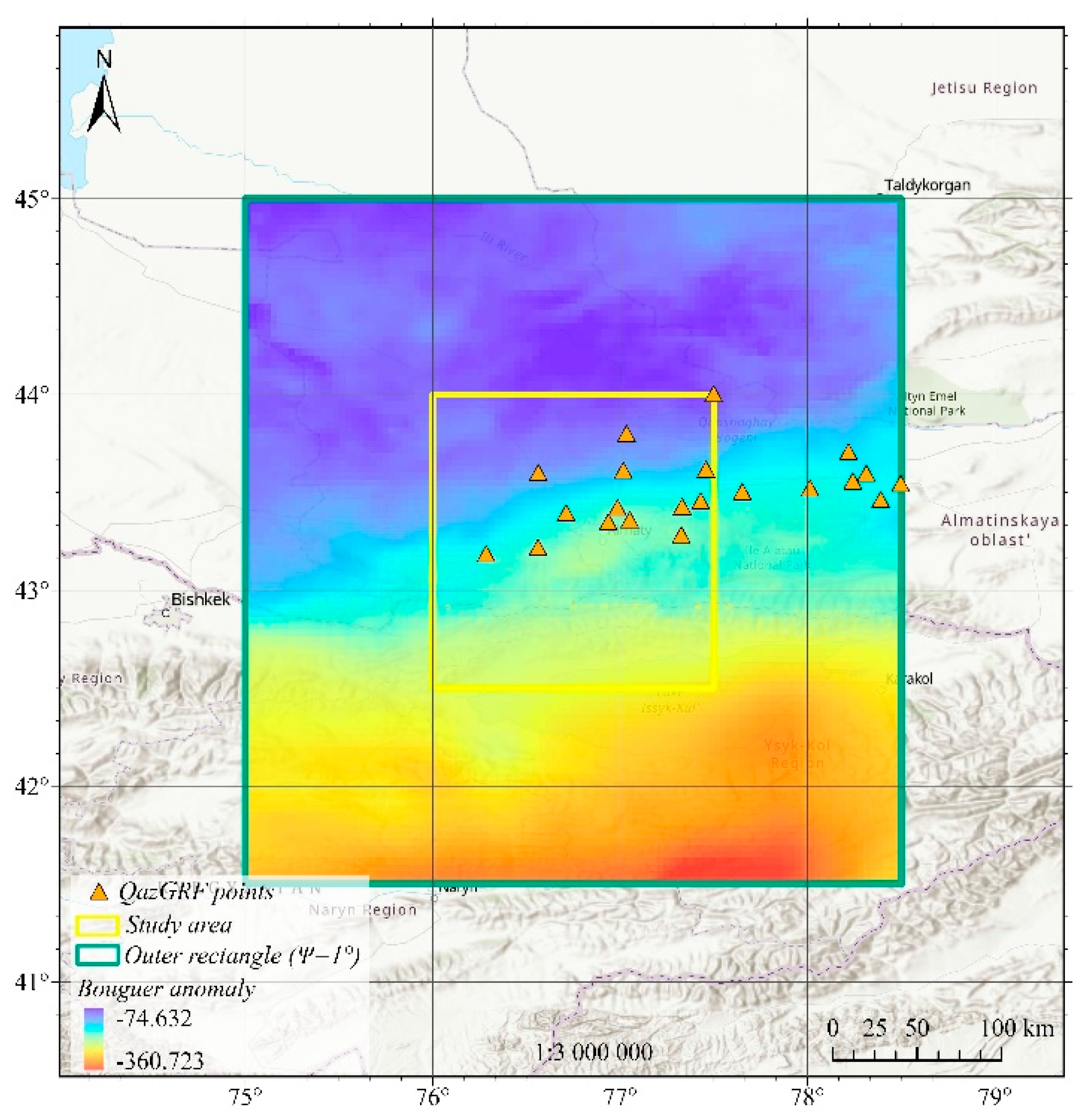
Figure 5.
Spatial distribution of GNSS/leveling benchmarks of II–III order.
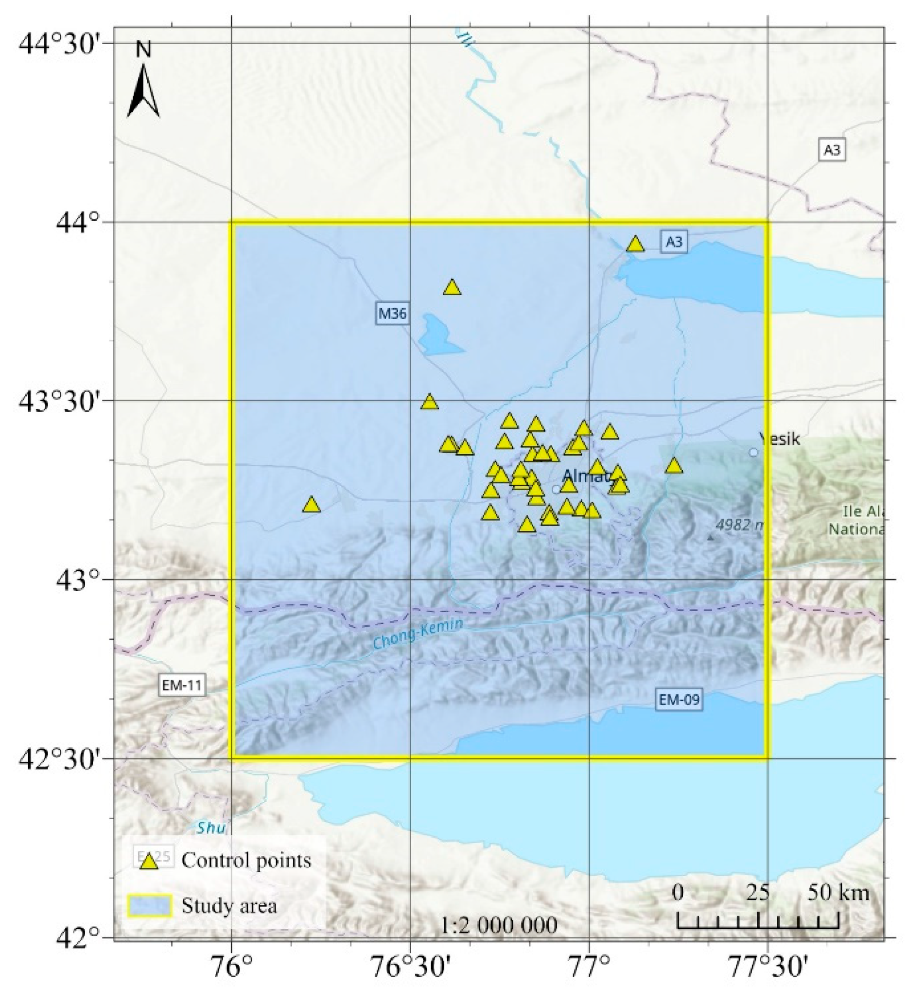
Figure 6.
Stages of the full GNSS post-processing cycle.
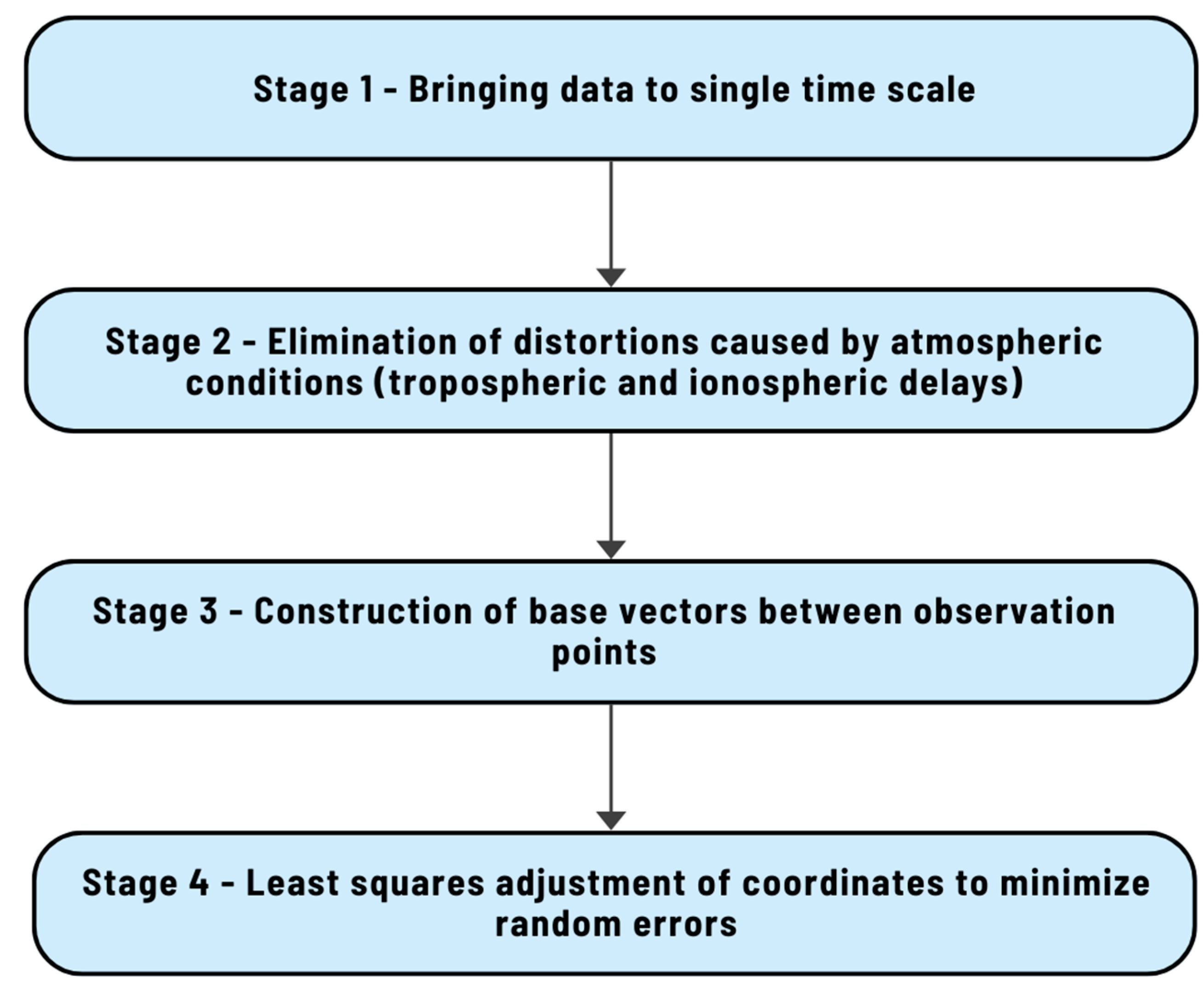
Figure 7.
Workflow of the hybrid geoid modelling.
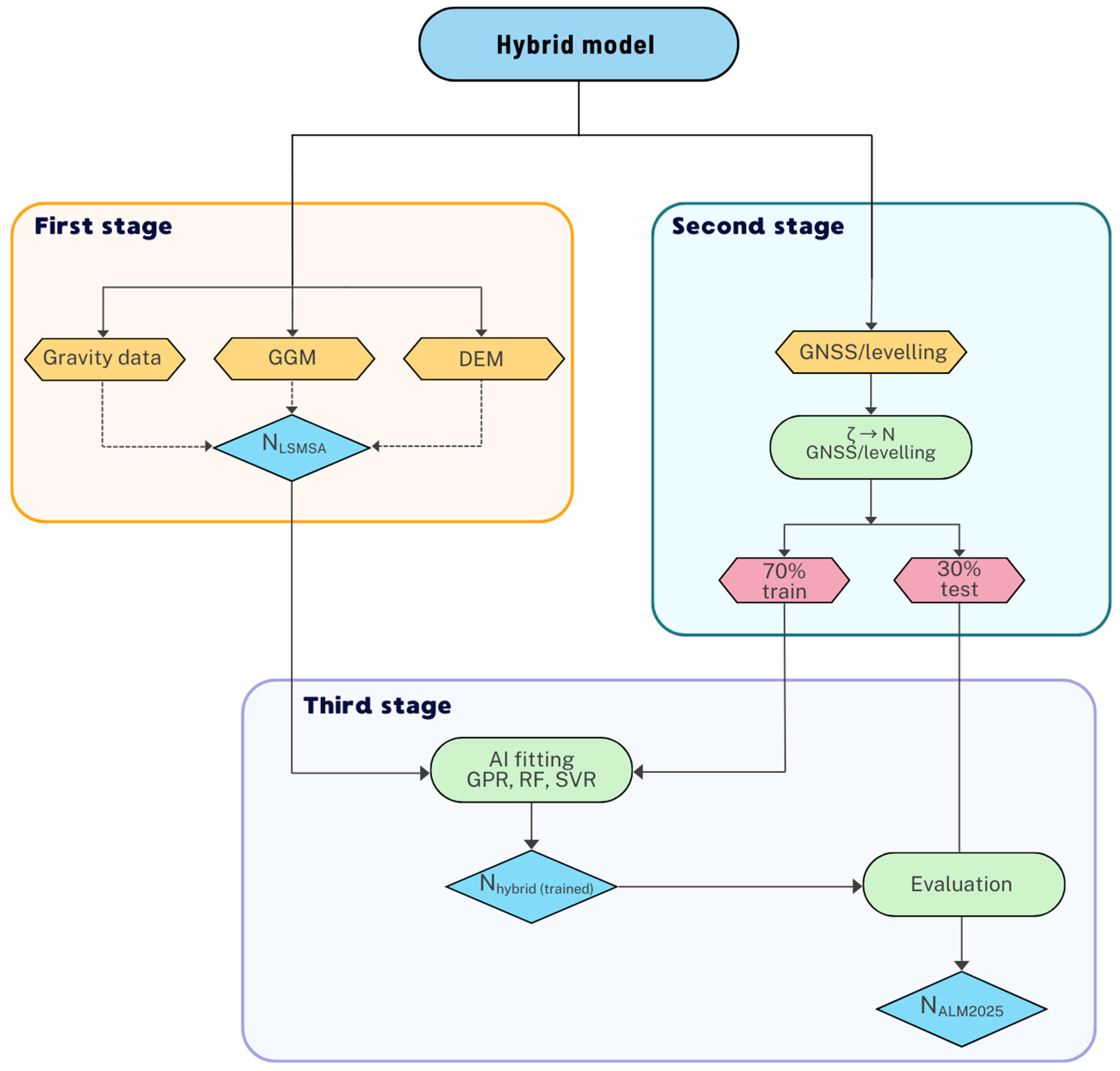
Figure 8.
Graph of the change in statistics with decreasing degree of GGM with the variance of errors of ground gravity data C (0) =1 mGal2.
Figure 8.
Graph of the change in statistics with decreasing degree of GGM with the variance of errors of ground gravity data C (0) =1 mGal2.
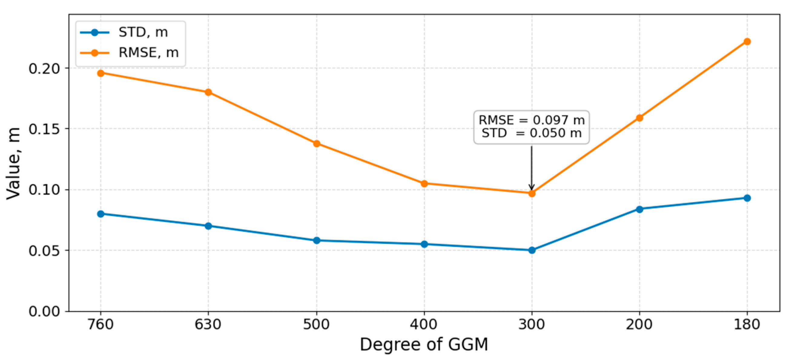
Figure 9.
Approximate geoid heights without corrections Napp, m.
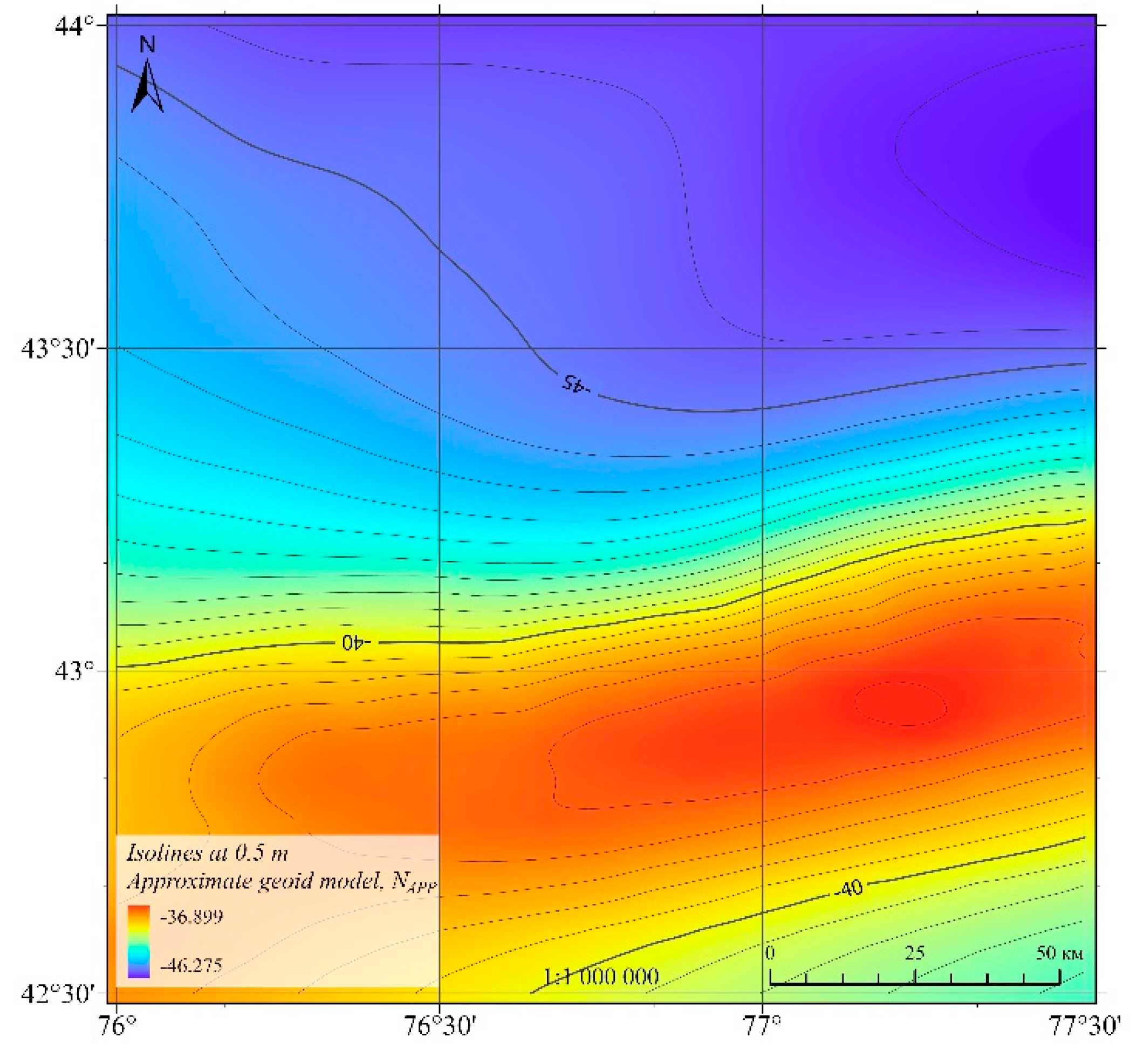
Figure 10.
Corrections to approximate geoid heights using: (a) topographic correction, m; (b) correction for analytical downward continuation, m; (c) ellipsoidal correction, mm; (d) atmospheric correction, mm.
Figure 10.
Corrections to approximate geoid heights using: (a) topographic correction, m; (b) correction for analytical downward continuation, m; (c) ellipsoidal correction, mm; (d) atmospheric correction, mm.
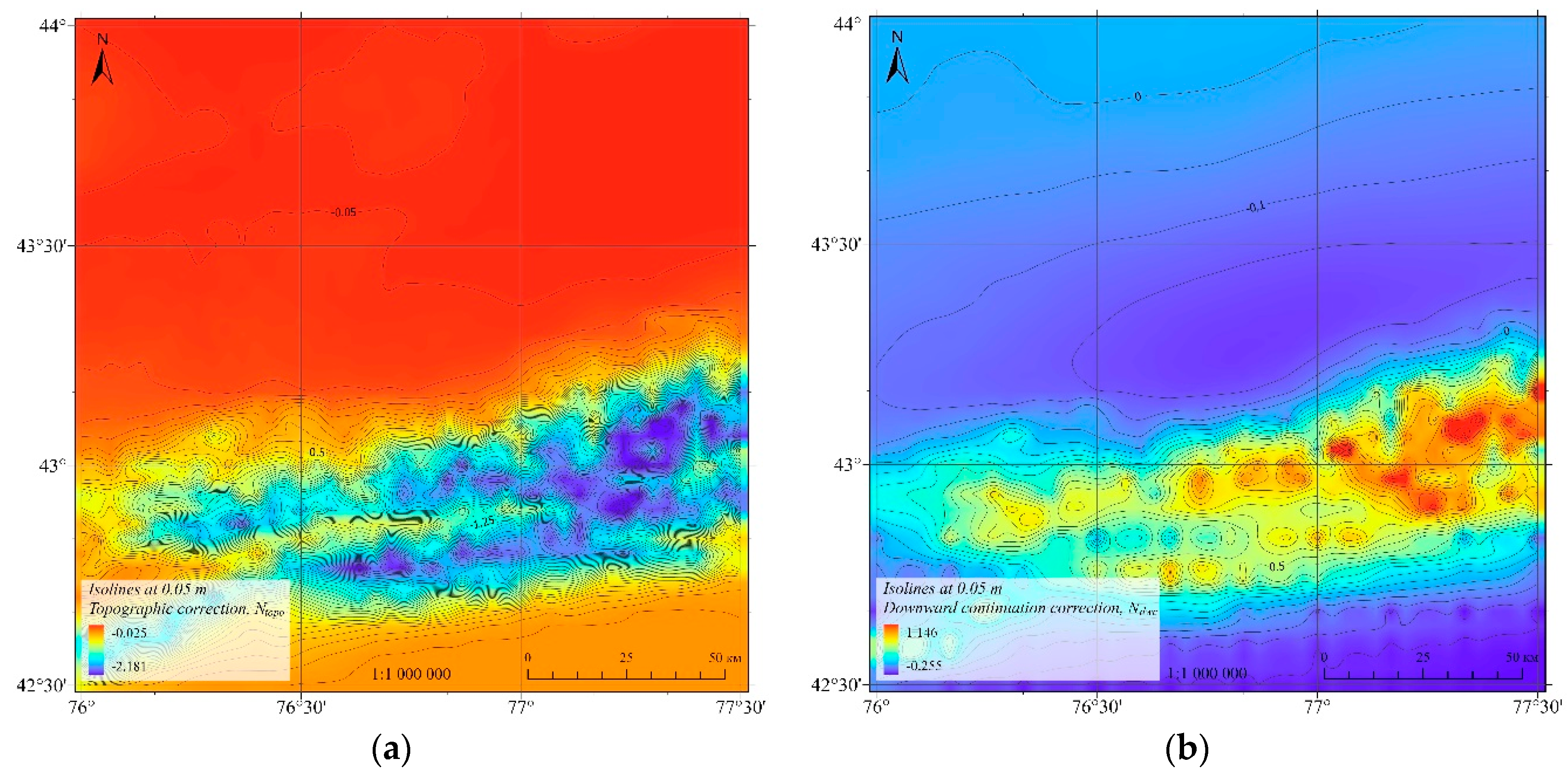
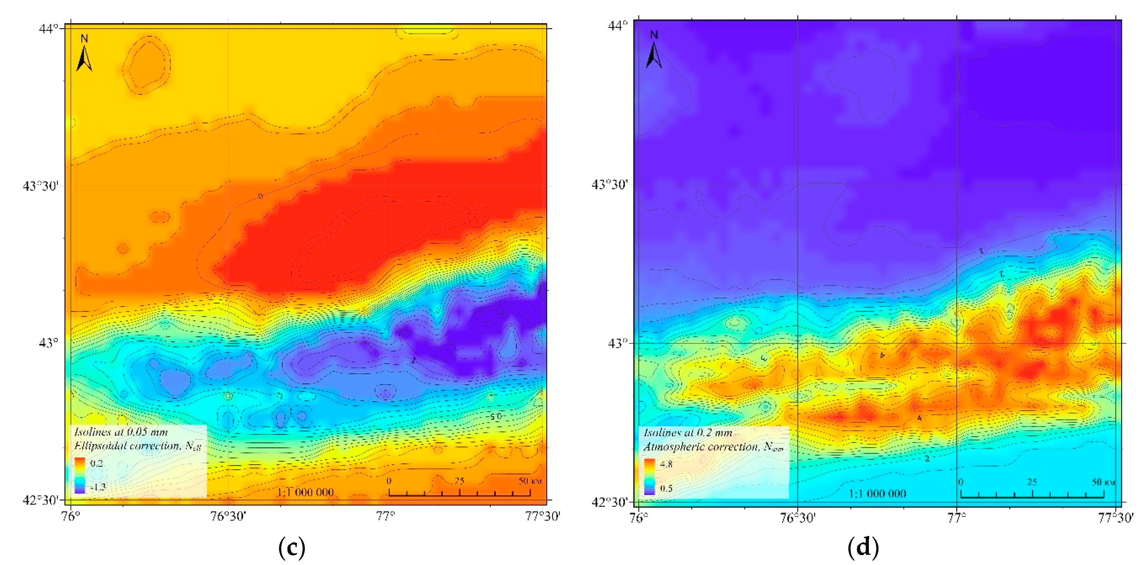
Figure 11.
Geoid height by the method of Least Squares Modification of Stokes formula with additional corrections N LSMS , m.
Figure 11.
Geoid height by the method of Least Squares Modification of Stokes formula with additional corrections N LSMS , m.
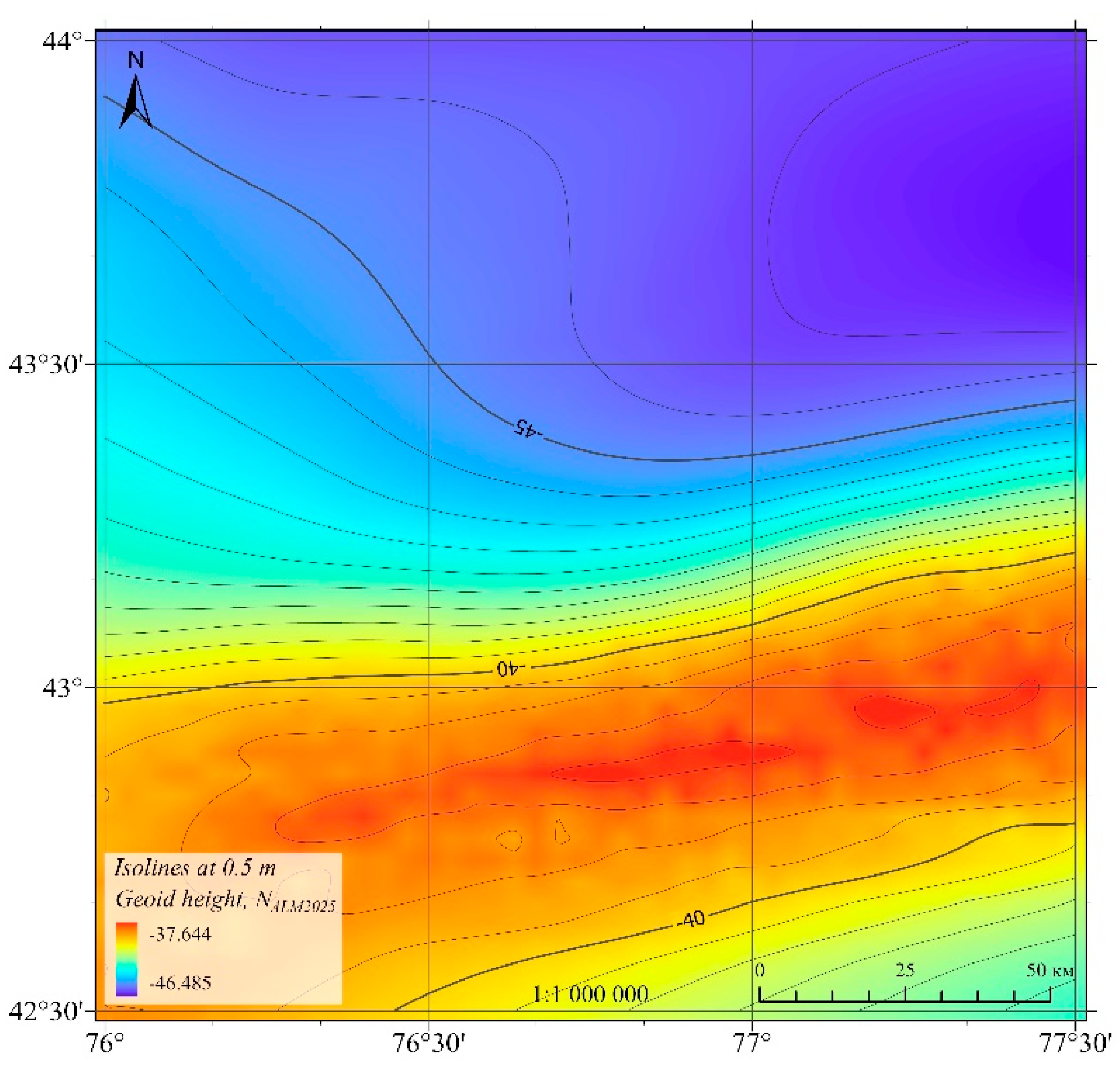
Figure 12.
Histograms of geoid residuals before and after SVR-based correction, m.
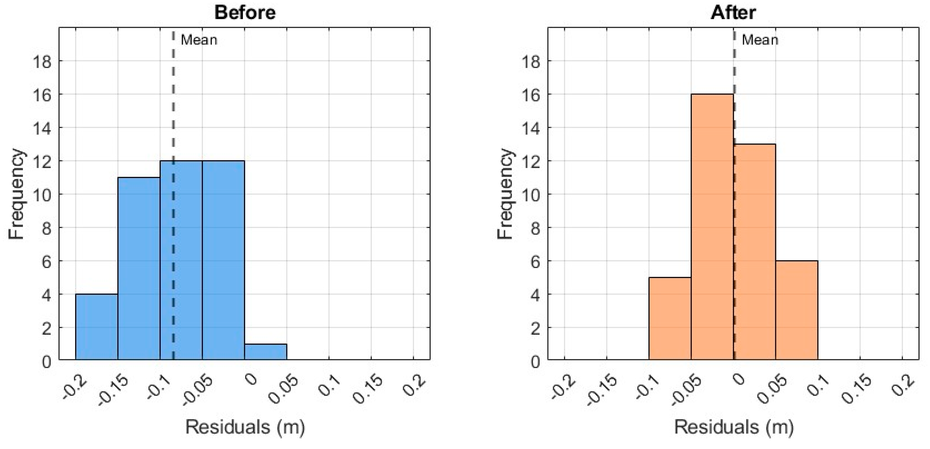

Table 1.
Statistics for fitting a combination of spherical harmonic coefficients with error variance of ground gravity data (m).
Table 1.
Statistics for fitting a combination of spherical harmonic coefficients with error variance of ground gravity data (m).
| C(0), mGal2 | ||||||||||
|---|---|---|---|---|---|---|---|---|---|---|
| 16 | 9 | 6 | 3 | 1 | ||||||
| Mmax | STD | RMSE | STD | RMSE | STD | RMSE | STD | RMSE | STD | RMSE |
| 760 | 0.252 | 0.472 | 0.200 | 0.390 | 0.167 | 0.339 | 0.122 | 0.270 | 0.080 | 0.196 |
| 630 | 0.190 | 0.349 | 0.156 | 0.312 | 0.133 | 0.283 | 0.101 | 0.238 | 0.070 | 0.180 |
| 500 | 0,100 | 0.196 | 0.085 | 0.182 | 0.070 | 0.165 | 0.058 | 0.138 | ||
| 400 | 0.066 | 0.142 | 0.055 | 0.105 | ||||||
| 300 | 0.050 | 0.097 | ||||||||
| 200 | 0.084 | 0.159 | ||||||||
| 180 | 0.093 | 0.222 | ||||||||
Table 2.
Statistics of applied additive corrections.
| Correction Type | Min | Max | Mean | STD |
|---|---|---|---|---|
| Topographic | −2.181 m | −0.025 m | −0.421 m | 0.534 m |
| DWC reduction | −0.255 m | 1.147 m | 0.042 m | 0.245 m |
| Ellipsoidal | −1.3 mm | 0.2 mm | −0.3 mm | 0.3 mm |
| Atmospheric | 0.5 mm | 4.8 mm | 1.7 mm | 1.2 mm |
| Sum of all corrections | −1.652 m | −0.020 m | −0.378 m | 0.331 m |
Table 3.
Residual error statistics for geoid correction across ALL/TRAIN/TEST (m).
| Method | Split | N | Mean | Median | STD | RMS | MAE | IQR | MIN | MAX |
|---|---|---|---|---|---|---|---|---|---|---|
| BEFORE | ||||||||||
| None | ALL | 40 | -0.084 | -0.091 | 0.050 | 0.097 | 0.084 | 0.080 | -0.186 | 0.001 |
| TRAIN | 28 | -0.080 | -0.079 | 0.053 | 0.095 | 0.080 | 0.076 | -0.186 | 0.001 | |
| TEST | 12 | -0.093 | -0.098 | 0.044 | 0.102 | 0.093 | 0.057 | -0.145 | -0.008 | |
| AFTER | ||||||||||
| Helmert | ALL | 40 | 0.035 | 0.009 | 0.134 | 0.135 | 0.054 | 0.044 | -0.058 | 0.604 |
| TRAIN | 28 | 0.000 | 0.005 | 0.033 | 0.031 | 0.026 | 0.048 | -0.058 | 0.048 | |
| TEST | 12 | 0.123 | 0.038 | 0.236 | 0.248 | 0.123 | 0.036 | 0.006 | 0.604 | |
| GPR (ARD-SE) | ALL | 40 | -0.003 | -0.000 | 0.025 | 0.025 | 0.011 | 0.000 | -0.064 | 0.074 |
| TRAIN | 28 | 0.000 | 0.000 | 0.000 | 0.000 | 0.000 | 0.000 | -0.000 | 0.000 | |
| TEST | 12 | -0.010 | -0.015 | 0.046 | 0.045 | 0.038 | 0.050 | -0.064 | 0.074 | |
| SVR (RBF) | ALL | 40 | -0.006 | -0.003 | 0.039 | 0.039 | 0.028 | 0.029 | -0.113 | 0.076 |
| TRAIN | 28 | -0.008 | 0.004 | 0.042 | 0.042 | 0.030 | 0.047 | -0.113 | 0.076 | |
| TEST | 12 | -0.002 | -0.006 | 0.034 | 0.032 | 0.024 | 0.031 | -0.073 | 0.058 | |
| LSBoost | ALL | 40 | 0.000 | -0.000 | 0.023 | 0.022 | 0.012 | 0.004 | -0.070 | 0.076 |
| TRAIN | 28 | 0.000 | -0.000 | 0.005 | 0.005 | 0.003 | 0.002 | -0.011 | 0.015 | |
| TEST | 12 | 0.001 | 0.004 | 0.042 | 0.040 | 0.033 | 0.058 | -0.070 | 0.076 | |
Disclaimer/Publisher’s Note: The statements, opinions and data contained in all publications are solely those of the individual author(s) and contributor(s) and not of MDPI and/or the editor(s). MDPI and/or the editor(s) disclaim responsibility for any injury to people or property resulting from any ideas, methods, instructions or products referred to in the content. |
© 2025 by the authors. Licensee MDPI, Basel, Switzerland. This article is an open access article distributed under the terms and conditions of the Creative Commons Attribution (CC BY) license (http://creativecommons.org/licenses/by/4.0/).
Copyright: This open access article is published under a Creative Commons CC BY 4.0 license, which permit the free download, distribution, and reuse, provided that the author and preprint are cited in any reuse.


