
Submitted:
14 September 2024
Posted:
16 September 2024
You are already at the latest version
Abstract
Quantifying forest carbon storage to better manage climate change and its effects requires accurate estimation of forest structural parameters such as canopy height. Variables from remote sensing data and machine-learning models are tools that are being increasingly used for this purpose. This study modelled canopy height of forest-savannah mosaics in the Sudano-Guinean zone of Togo. Relative heights were extracted from GEDI and ICESat-2 products, which were combined with optical, radar and topographic variables for canopy height modelling. We tested four methods: Random Forest (RF); Support Vector Machine (SVM); Extreme Gradient Boosting (XGBoost); and Deep Neural Network (DNN). The RF algorithm obtained the best predictions using 98% relative height (RH98). The best performing result was obtained from variables extracted from GEDI data (r = 0.84; RMSE = 4.15 m; MAE = 2.36 m), compared to ICESat-2 (r = 0.65; RMSE = 5.10 m; MAE = 3.80 m). Models that were developed during the study, from the combination of multisource and multisensor data, can be applied over large areas in forest-savannah mosaics, thereby contributing to better monitoring of forest dynamics according to the objectives and requirements of REDD+.
Keywords:
Spatial LiDAR
; GEDI
; ICESat-2
; canopy height
; modelling
; data combinations
; forest-savannah mosaics
1. Introduction
The rapid rise in global greenhouse gas (GHG) emissions since the debut of the Industrial Revolution has led to considerable changes in the Earth’s climate, which has been the subject of much research over recent decades. The Intergovernmental Panel on Climate Change (IPCC) has determined that this increase in anthropogenic GHG emissions is the primary driver of climate change, which can push temperatures beyond the thermal tolerances of many species [1,2]. According to current trends, global warming that is linked to these gases will likely exceed 1.5 °C within several decades, despite aggressive emissions reduction strategies [3]. Removing CO2 from the atmosphere by favouring nature-based solutions (protected areas and forests) could contribute greatly to climate change mitigation [4,5,6].
Forests constitute one of the largest reservoirs of terrestrial carbon, thereby playing a vital role in offsetting the aforementioned climate changes and regulating global carbon balance. Annually, they contribute to about 50% of net terrestrial primary production, store about 45% of the planet's active carbon, and sequester around 33% of anthropogenic emissions [7,8,9]. Unfortunately, tropical forest ecosystems, which maintain the global ecological equilibrium, are constantly threatened by deforestation and degradation for economic purposes. Timber extraction and forest clearing for other land uses are among the largest sources of anthropogenic carbon emissions [10]. In this context, the implementation of the Paris Agreement on climate change and the 2030 Agenda for Sustainable Development (adopted in 2015) by UN member nations require quantitative studies that would provide essential data for monitoring forest dynamics [11,12,13].
Canopy height is one of several structural parameters that is used to monitor these forest dynamics. Its precise estimation is crucial for quantifying biophysical parameters, such as aboveground biomass, carbon storage, biodiversity, and many other parameters to which it is strongly linked [14,15,16]. Traditional methods of estimating forest height are based upon manual forest inventories, which are conducted in the field. While these inventories can provide accurate detailed information, they are very labour-intensive, time-consuming, and may cover only small spatio-temporal scales. Consequently, remote sensing has been employed in recent decades, in combination with field measurements, to estimate canopy height over large spatial extents [17,16]. The remote sensing observations are provided by various platforms. These include for instance multi-spectral optical data that are derived from Landsat [18,19], Sentinel 2 [20,21], or SPOT5 [22,23], as well as synthetic aperture radar (SAR) data from Sentinel 1 [24,25], TerraSAR-X [26,27], TanDEM-X [28,29] or ALOS PALSAR [30,31]. Regardless of whether the data are optical or obtained from radar, signal saturation (especially in dense forests) can constitute a substantial limitation [32,33,34,35]. The introduction of LiDAR (Light Detection And Ranging) has enabled notable advances in the estimation of canopy height, because of their capacity to detect vertical structure in the forest [16]. The most frequently used applications in forestry are based on telemetry from airborne laser scanning (ALS) [36,37] and terrestrial laser scanning (TLS) [38,39]. However, ALS and TLS exhibit spatio-temporal limitations, given that it is generally difficult to apply them over large areas and on a regular basis, due to their high costs of acquisition and to signal occultation, particularly in dense forests [40,41,42,43].
Airborne or satellite platforms have made it possible to extend canopy height estimation from local to global spatial scales [13]. The first platform, i.e., Ice, Cloud, and land Elevation Satellite (ICESat) carried the Geoscience Laser Altimeter System (GLAS). Between 2003 and 2009, this sensor made it possible to estimate the height of forests on a global scale on circular footprints with a diameter of about 60 m and a spacing of about 170 m along the transects [44,45,46,9]. The second ICESat-2 satellite was launched in September 2018 and carried the Advanced Topographic Laser Altimetry System (ATLAS), which uses photon-counting LiDAR technology. Between 88◦ S and 88◦ N, the laser produces three pairs of beams, thereby making it possible to obtain altimeter parameters on Earth’s surface for continuous monitoring of polar glaciers. In parallel with its main mission, this satellite also acquired terrestrial measurements of forest cover and vegetation. For the scientific community, this represents an important database for mapping plant biomass and for estimating carbon inventories at a global level [47,17]. The latest LiDAR instrument that was launched into space by NASA in December 2018 is the Global Ecosystem Dynamics Investigation (GEDI) system, which operates aboard the International Space Station (ISS) between 51.6◦ N and 51.6◦ S. GEDI is a multi-beam laser altimeter that measures parameters of vertical canopy structures at a very high sampling rate, thereby allowing forest height and wood volume estimation across different types of forest ecosystems, topography and latitudes [13]. Data that are acquired by GEDI have been increasingly used to estimate forest height and forest biomass [48,49,50]. These data consist of an impressive number of samples, which offer great potential for estimating canopy heights in complex savannah and forest mosaics.
ICESat-2 and GEDI LiDAR data are point clouds that permit the height of forest cover to be estimated, but only within ground acquisition footprints, rather than in a spatially continuous manner over large areas [51]. In contrast, optical or radar data provide continuous spatial coverage; but cannot, alone, allow the direct extraction of vertical profiles of the canopy. Therefore, the complementarity of different types of data can be exploited to map the height of the forest cover [52,53,54,55]. To accomplish this task, machine-learning models are being increasingly used to combine vertical LiDAR profiles with spectral or backscatter attributes [56,16]. For example, Li et al. [15] used variables derived from Sentinel 1&2 and Landsat-8 images over Northeast China to extrapolate ICESat-2 canopy height from the footprint-level to regional-level, using Deep Learning (DL) and Random Forest (RF) models, with correlations of (r =) 0.78 and 0.68, respectively. Zhu et al. [9] used stepwise regression and Random Forest (RF) approaches to estimate canopy heights in the United States. They obtained better results with RF using GEDI variables (R2 = 0.93; RMSE = 2.99 m) compared to those of ICESat-2 (R2 = 0.78; RMSE = 4.62 m). Sothe et al. [57] carried out continuous mapping of the forest cover height of Canada from the combination of GEDI and ICESat-2 data with PALSAR and Sentinel data. They found that both LiDAR products overestimated canopy height compared to ALS data, but GEDI outperformed ICESat-2, with an average difference of 0.9 m vs. 2.9 m and RMSE of 4.2 m vs. 5.2 m, respectively. To map China's forest canopy heights, Liu et al. [58] used neural network-guided interpolation to merge GEDI and ICESat-2 data. They then compared the height of the forest cover that was interpolated with the GEDI validation footprints (R2 = 0.55; RMSE = 5.32 m), followed by drone-LiDAR validation data (R2 = 0.58, RMSE = 4.93 m) and, finally, with field-collected data (R2 = 0.60; RMSE = 4.88 m).
The aforementioned examples show real potential for using GEDI and ICESat-2 data alone or in combination with other spatial data. However, they also raise several questions, which depend upon the ecosystems that are being considered. Of particular interest is the following: Can the use of GEDI or ICESat-2 data (alone or in combination) with multisource optical or radar satellite observations make it possible to estimate satisfactorily the canopy heights of complex mosaics of forests and savannahs in a tropical environment? Our study attempts to answer the question through analyses of the forest-savannah mosaics of the Sudano-Guinean zone of West Africa, particularly in Togo, where research of this type is almost non-existent. Our main objective is to develop models for estimating height of the canopy in forest-savannah mosaics using a combination of space LiDAR, optical data and radar data. The specific objectives that we pursued are: 1) to analyze the performance of covariates and ICESat-2 and GEDI data in predicting canopy height in these forest ecosystems; 2) to develop canopy height prediction models that are adapted to forest-savannah mosaics; and 3) to establish continuous mapping of canopy height in these forest types from these discontinuous satellite LiDAR data. To accomplish these goals, optical and radar co-variables, such as spectral reflectances, vegetation indices, texture and backscatter variables, are derived from the spatially continuous satellite data, which were then integrated with those derived from ICESat-2 and GEDI, using machine-learning models.
2. Materials and Methods
2.1. Study Aera
Our study was conducted in Ecological Zone 4, southwest Togo. The Togolese Republic is a coastal nation in West Africa that is bordered on the north by Burkina Faso, by the Atlantic Ocean (Gulf of Guinea) to the south, by Benin to the east, and by Ghana to the west. The country is subject to a tropical Sudano-Guinean climate, with rainfall varying across four seasons from 1000 to 1600 mm/year in the southern regions. Average temperature is 27 °C [59]. Between 1939 and 1957, the classification of 14.2% of the country’s land area into protected areas (classified forests, national parks and reserves) served to preserve its forest cover. Today, many of these areas have been encroached by human populations seeking arable land and wood for energy. Vegetation types are composed of Sudano-Guinean forests, which are located in mountainous areas of the country, gallery forests along the main waterways, dry forests or dense tree savannahs in the arid northern half, and tree savannahs in the south and center. Five ecological zones have been designated, spanning the country.
Located in the southern Togo Mountains, Ecological Zone 4 (6397 km2), is one of such subdivision that is characterized by the landscape variability of its ecosystems [60]. Always known as the most heavily forested of the country’s ecological zones, Zone 4 is dominated by interspersed semi-deciduous forest and mosaics of Guinean savannah, with the latter having been degraded in recent years by the combined effects of slash-and-burn agriculture, vegetation fire and logging [61,62]. Over the past three decades, the zone has lost more than 27% of its forest cover, yet it remains the most forested and least degraded of the country's five ecological zones [63]. The study area is presented in Figure 1.
2.2. Methodology
To develop canopy height prediction models, multisource variables were extracted from the collected data, and made usable during models’ development process. Modelling involves the use of relative canopy heights and other variables that have been extracted from satellite LiDAR data (GEDI and ICESat-2), together with those that have been extracted from spatially continuous data. After the preprocessing stage, prediction variables were extracted from radar (Sentinel 1), optical (Sentinel 2) and topographical (SRTM) data. The former consist of native bands, vegetation indices, texture measurements and topographical variables. The methodological flowchart of this study using these data is illustrated in Figure 2.
2.3. Data Acquisition
The data that were collected and organized prior to use in this research come from seven sources (see Figure 2), separated into two main categories. The first category concerns remote sensing data, notably optical, radar, topographical and satellite LiDAR sources; the second category consists of dendrometric field data. The general parameters of these data sources data are summarized in Table 1, while the variables that are extracted and their extraction methods are described in Section 2.4.
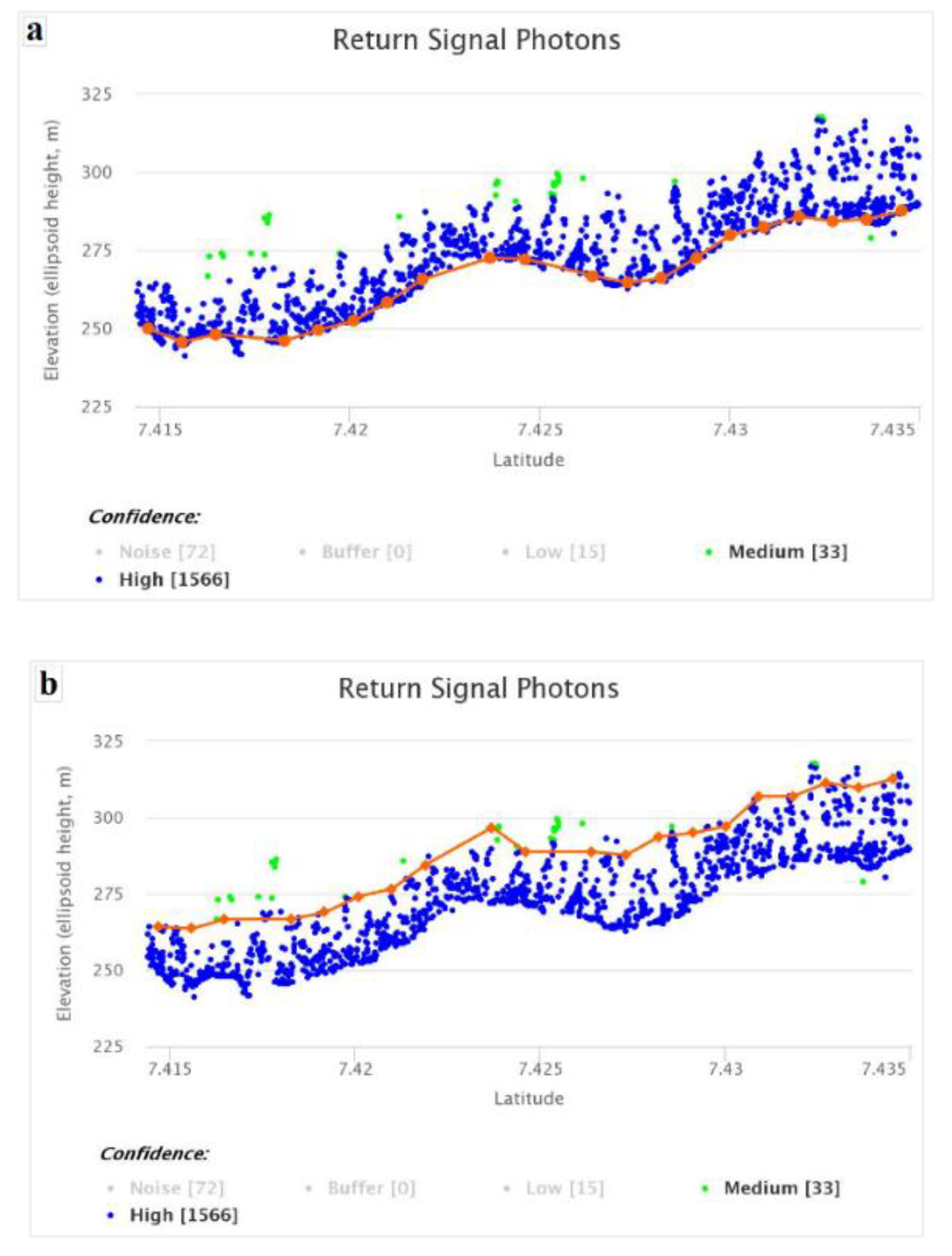
Spatially discontinuous data from the Global Ecosystem Dynamics Investigation (GEDI) and Ice, Cloud, and Land Elevation Satellite-2 (ICESat-2) satellites have been downloaded from NASA's Land Processes Distributed Active Archive Center (LPDAAC) website (https://lpdaac.usgs.gov/). It should be noted that GEDI data are products of the International Space Station (ISS). The granules are GEDI data reduced size from one full ISS orbit to four segments per orbit [66]. The structures of the ground footprints of these satellite LiDAR data are illustrated in Figure 3a and Figure 3b, for ICESAt-2 and GEDI, respectively. Figure A1 (Appendix A) shows elevations of the ground surface (a) and canopy top (b) extracted from photon returns in ATL08 data acquired by ICESat-2 in the southwest of the city of Badou (7°35′8″N, 0°36′33″E). Continuous Sentinel 1, Sentinel 2 and SRTM data were collected from archives of the Google Earth Engine platform.
Regarding field data, a field campaign that was conducted between October 2020 and February 2021 made it possible to collect dendrometric field parameters within the rectangular footprints (17 m by 100 m) of the ICESat-2 data. Within these footprints, the total height was measured on the footprints using a Suunto clinometer and the diameter at breast height (DBH, 1.3 m) was measured using a direct diameter measurement tape, for all trees with a diameter greater than or equal to 10 cm. To supplement these data, we added measurements taken from the second National Forest Inventory (IFN2). An existing land use map from 2020 was also used in this study as auxiliary data to identify the most forested areas.
2.4. Variable Extraction
From Sentinel 1, Sentinel 2 and SRTM data, variables were extracted or calculated to serve as independent variables when predicting canopy height. The latter are made up of native bands, vegetation indices, texture measurements and topographical variables. They included 29 variables for radar data, 28 for optical data, and 3 for topographical data. We used JavaScript code when extracting these continuous variables. Table 2 contains the summary list of all variables that were resampled at 30 m resolution, particularly those variables which were not already measured at 30 m, so that they could be used with the other covariates.
Formulas used for calculating some variables, together with their respective references, are provided in Table A1 (Appendix B). From the GEDI L2A granules of the GEDI data, we extracted location parameters (latitude, longitude) and relative height values as percentiles (RH50, RH55, RH60, RH65, RH70, RH80, RH85, RH90, RH95, RH98 and RH100), which are frequently used for canopy height prediction. Other variables that are considered useful for modelling forest structure, such as beam type (coverage, full power), data quality indicator and sensitivity of the waveform to penetrate vegetation, were extracted. For the ICESat-2 data, we downloaded ATL08 products from which we extracted the powerful beams, representing the best option for detecting ground and canopy photons according to Neuenschwander and Pitts [67]. We used Matlab code when extracting these ICESat-2 and GEDI variables. Relative heights were also calculated for each of the plots, given that the field measurements were taken from individual trees.
2.5. Preparation of Variables for Modelling
Since the variables extracted from the data could not be used directly to develop the canopy height models, they were prepared for that purpose. This involved validating the relative heights, filtering the data and calculating zonal statistics.
2.5.1. Validation of Satellite LiDAR Data
In order to use the relative heights extracted from ICESat-2 data as predictors of canopy height, we validated them with those that were collected from their ground footprints. To this end, they were compared with those calculated from field data. Given that the field data were collected on individual trees, we first aggregated them into data which could be easily compared to those extracted from ICESat-2, by calculating their statistics per plot. For each plot, the statistics calculated from the field data are: the minimum, the maximum, the first quartile, the mean, the median, and relative heights of 50%, 55%, 60%, 65%, 70%, 75 %, 80%, 85%, 90%, 95% and 98%.
The variable that was extracted from the ICESat-2 data and used for this comparison with field data is the relative height at 98%, designated h_canopy. Once these field variables had been calculated, the latter were matched with them by plot in an Excel table, which was used to establish a correlation matrix. The Pearson correlation values obtained between the field variables and relative height, h_canopy, allowed to use it as reference data for modelling canopy height. It should be noted that this validation using field data only concerns ICESat-2, given that we did not have field data from the GEDI footprints to conduct a similar analysis.
2.5.2. Data Filtering
During variable preparation, the data were filtered using various parameters internal to the dataset. During extraction of relative heights, other variables were extracted from satellite LiDAR and auxiliary data to use them as filtering parameters to clean the database used for modelling.
- For the ICESat-2 data, the number of photons classified as canopy in the segments (n_ca_photons) and the spacecraft orientation tracking parameter (sc_orient) were considered. During filtering, the n_ca_photons parameter was used to eliminate all footprints with a low number of canopy photons, while the sc_orient parameter was used to identify the strong beams from the weak beams: When sc_orient is equal to 0, the satellite is ascending and the strong beams are on the left on the ground tracks, while the weak beams are on the right, whereas the opposite occurs when it is equal to 1.
- For GEDI data, the parameters used are the identifiers for the type of beam which can be coverage or full power (Beam), data quality indicator (Quality_flag), sensitivity of the waveform to penetrate vegetation (Sensitivity) and firing time (delta_time). Filtering using these parameters made it possible to select footprints according to the nine configurations that are presented in Table 3.
- The geographical coordinates extracted from the ICESat-2 and GEDI data were used to display them on a GIS land cover map to identify the land cover classes into which each of their footprints fell. This action made it possible to select footprints that fell into the forest classes, and to remove from the database those that fell into other classes such as "crops and fallow land", "buildings and bare soil" and "grassy savannah".
The data filtering stage therefore made it possible to remove from the database any values that could have added noise to the modelling process or which reduced the quality or performance of the prediction models being developed. Filtering in relation to the location of LiDAR data footprints in forest areas was conducted in ArcGIS 10.8.1. Filtering of other parameters that were extracted from LiDAR data was conducted using a Python code developed for this purpose.
2.5.3. Calculation of Zonal Statistics
To properly integrate the data during modelling, zonal statistics were calculated on the continuous variables from the ICESat-2 and GEDI data footprints. For each variable extracted from the Sentinel 1, Sentinel 2 and SRTM data, the mean, median and standard deviation of the pixel values were calculated for each footprint of the satellite LiDAR data superimposed upon it. These three calculated statistics were evaluated at the start of modelling to select the one that provided the most accurate canopy height prediction results. Figure 4 shows an example of the GEDI and ICESat-2 footprints superposed over Sentinel 1 for the calculation of zonal statistics.
For each of these variables, the statistics were matched with relative heights and other variables extracted from the satellite LiDAR data to form a table for each variable. These data tables per variable were then grouped by data source (optical, radar, topographic) to provide the databases used in modelling.
2.6. Modelling
Once the variables had been extracted and prepared, we proceeded with modelling, which consisted of variable selections, predictive model development, and evaluation. Given that these continuous variables provide different information, we analyzed different scenarios for combining them, as presented in Table 4, to make the best possible choices.
To explore the influence of height classes on modelling, we divided the data into two groups of height classes. Because of their small number, the data with canopy heights ≤ 5 m (]2 - 5]) formed the first class in these two groups. Group 1 contained 7 classes increasing in 5 m increments from the upper bound of the first class (i.e., (]2 - 5]), (]5 - 10]), (]10 - 15]), etc.). Group 2 contained 10 height classes in which the step size or increment was set at 3 m relative to the upper bound of the first class (i.e. (]2 - 5]), (]5 - 8]), (]8 - 11]), etc.). Like the first class, canopy heights > 30 m (]30 – 50]) constituted a separate class in each of the two groups. When data were filtered (see Section 2.5.2), individuals with heights < 2 m or > 50 m were deleted from the database with reference to the field data.
The database created in the previous step is such that , where , is the set of sampled GEDI or ICESat-2 footprints, represents the set of extracted attributes, and represents the canopy height value that was extracted from the observations of GEDI or ICESat-2 footprints. With these input data (), one part ( = 80%) trained the models, and the other part ( = 20%) tested these models to evaluate their performance.
2.6.1. Variable Selection
In this study, the importance of variables was determined using the RF variable importance approach. Decision trees (DTs) of the RF model and the nodes that link them provide information about the contributions of the input variables used in prediction, and it is this information that enables their importance to be assessed. When an upper node (parent node) is divided into two lower nodes (child nodes) by the variable i, the importance of the variable is defined as the difference between the root-mean-square error (RMSE) of the parent node and the sum of the RMSEs of the child nodes [68]. According to Hwang et al. [68], the importance of variable i for a given decision tree is defined by equation 1 below.
where is the information gain of node j branched by the variable i and of all nodes. The importance of each variable can then be normalized according to the following equation (2):
Finally, the importance of each variable in the RF model is averaged over all decision trees in RF as in equation 3:
where is the importance of variable i in the RF model and is the total number of decision trees in RF. Ranking all the variables, therefore, allows us to retain only those with the highest values of .
When testing the four modelling algorithms, we also used the SHAP (SHapley Additive exPlanations) method [69,70], which allowed us to select certain predictors with much greater effects on the performance of the models. This method is a game-theoretic approach that explains the predictions of machine-learning models and, thus, facilitates their interpretation [71,72].
2.6.2. Development of Prediction Models
We evaluated four machine learning algorithms, namely Random Forest (RF), Support Vector Machine (SVM), Extreme Gradient Boosting (XGBoost), and Deep Neural Network (DNN). The goal was to assess their relevance in order to select the best model, which was optimized using an automated learning tool. The objective is to construct a model according to the equation:
with representing parameters and hyperparameters of the model to be learned and is predicted height. This model should be capable of predicting the height that minimizes the cost function:
where represents the loss function. Equation (5) is a general form of the loss function, but here we have used root-mean-square error (RMSE) as the measure of loss. The four tested algorithms are briefly presented below.
- Random Forest
RF is a learning algorithm that constructs a series of decision trees generated by training samples taken at random with or without replacement. It uses the decision trees as the training base, where j is the number of base trees. Given the training database that is defined above for a particular realization of (with ), the trained decision tree is defined by . Although this formulation follows Breiman [73], the random realization is implicitly used to introduce randomness in two ways. First, "bagging" fits each tree to a randomly drawn sample of the original database. Second, when splitting a node, the best split is found on a randomly selected subset of p predictors rather than all predictors, independently at each node.
Decision trees are then constructed without being pruned; the resulting trees are combined as a weighted average, which is presented in equation 6.
Although the RF algorithm has demonstrated its prediction ability, three parameters can be adjusted to improve its performance, depending on the situations and applications. These are the number of predictive variables that are randomly selected at each node (p), the number of trees in the random forest (J) and the size of the tree [74].
- Support Vector Machine
The SVM algorithm is a supervised, non-parametric statistical learning technique, the initial purpose of which was to solve binary classification problems, which was later extended to regression problems [75]. The objective here is to model a function that would allow us to predict canopy height while maximizing the hyperplane, i.e., the margin between the predicted value () and the actual value (h), for all the training data. In the case of a non-linear support vector regression approach, this involves applying a transformation () from the space of the input data to a higher dimensional space in order to better predict the input data. Note that and are respectively dimensions of the space of the input data and transformed with . A kernel function such as a radial basis function is generally used to solve the non-linearity problem [76,77]. From then on, linear regression in dimensional space will be written as follows:
where is the hyperplane coefficient vector; is a scalar denoting bias.
- Extreme Gradient Boosting
The XGBoost algorithm is a machine-learning ensemble model, which is an efficient and scalable implementation of the gradient boosting machine algorithm [78]. As a learning set approach XGBoost uses multiple decision trees to achieve optimal prediction performance. The output of the model predicted by this approach will have the same decision rules as a classical decision tree model. Let K be the number of trees used, and the output prediction result is the sum of all the scores predicted by K trees, as shown in equation (8):
XGBoost adopts the same gradient boosting as the Gradient Boosting Machine (GBM) algorithm [79], but provides a small improvement to the objective function by regularizing it, as presented in equation (9):
Here, is the total objective function, represents the hyperparameters of the model, ℓ is a differentiable convex loss function which measures the distance between the prediction and the true value , the second term representing the regularization which reduces the variation in output of the new tree. Detailed information regarding the XGBoost model can be found in the literature [80,81].
In order for the model to work efficiently, XGBoost also stores data in in-memory units for parallel learning, thereby allowing it to handle larger datasets and to run much more rapidly [80].
- Deep Neural Network
DNN is a neural network that is organized into several hidden and densely connected layers, which characterize the input-output parameters of the network [82]. DNNs were selected because this architecture guarantees a high capacity for finding relationships between variables and for generating machine learning based on data representations [83]. The capacity that characterizes DNN is based upon the fact that each layer is continuously updated by repetitive learning, which is referred to as "backpropagation", to find the appropriate weights and biases [83]. Backpropagation is carried out until the difference between the predicted value and real value (the error) is optimal. In this perspective, the output (Oj) of the DNN layer j is defined according to equation 10, considering the input X (X = {x1, . . ., xN}) the activation function (σ), the weight matrix (w) and the bias vector (b)
This output is accurately predicted through careful adjustment of parameters, such as the activation function, the learning rate, number of neurons in each hidden layer, the number of hidden layers, batch size, and number of epochs, i.e., the number of forward-backward passes through the dataset [47], [84,85,86].
When using Machine Learning (ML) algorithms, it is sometimes difficult to manually identify the best hyperparameters for good model training or generalization [87,88]. To achieve this goal, the ML community has used approaches such as grid search and random search [89] or Bayesian optimization [90]. Yet, these ML models are configured by a set of hyperparameters with values that can substantially affect their performance, which means that we cannot know whether a given technique is truly better or simply better tuned [91,92]. Automated machine learning (AutoML) approaches automate the selection of algorithms and the implementation of other parallel operations to efficiently optimize hyperparameters, while taking into account the particularities of the input data. For this purpose, we employed the AutoML TPOT (Tree-based Pipeline Optimization Tool) and AutoGluon to compare their performance with that of the algorithm, which offered the most accurate results among the four being tested [93,94].
2.6.3. Performance Evaluation of the Developed Models
ICESat-2 canopy height was validated using Pearson's Correlation Coefficient (r) with reference to the measurements, before being used as reference data for canopy height prediction modelling. The prediction models and canopy height maps that were subsequently produced were evaluated, comparing one to another, and with existing models. The comparisons were made using traditional performance indicators, i.e., correlation r, RMSE (Root-Mean-Square Error) and MAE (Mean Absolute Error) to retain the models that stood out in terms of their performance. Equations 11 to 13 show the mathematical expressions of the three indicators:
where represents the ith observed value of the canopy height data extracted from ICESat-2 or GEDI, and is the ith predicted value; and are respectively the means of all and , while represents the total number of canopy height samples from ICESat-2 or GEDI.
These parameters were used to validate models developed from ICESat-2 data on the basis of data collected in the field from their footprints. The same parameters were calculated to evaluate model performance by comparing predicted canopy heights on the plots of the second National Forest Inventory (NFI2) with those measured in the field during the inventory. They also enabled us to compare the cartographic products of this study with those of other authors.
2.7. Forest Height Mapping
Following evaluation of the models developed, those obtaining the best performance in predicting canopy height on the satellite LiDAR footprints were retained for cartographic inference. Indeed, the execution of these models yielded predicted canopy heights in only LiDAR footprints, leaving blank areas between them. To move from spatially discontinuous to continuous data, we first created a stacked multi-band image, using the variables that had contributed the most to prediction, according to variable importance defined in Section 2.6.1. Given that each band in this stacked image was considered a predictor, execution of the trained model uses the content of each pixel and their corresponding values in the underlying bands, to produce a new height pixel. Several iterations of the process on all pixels of the stacked image complete the image of the heights that is produced. Figure 5 illustrates the cartographic inference that is performed with the models, which were developed from GEDI or ICESat-2 data.
The resulting canopy height maps were formatted in ArcGIS. To analyze differences between types of LiDAR data that were used, some statistical metrics of the map resulting from cartographic inferences with the GEDI-based model were compared with those obtained with the ICESat-2-based model. These two maps were compared to similar data existing locally or globally to obtain an understanding of the particularities that are related to our study area. The performance evaluation parameters that are presented in Section 2.6.3 were also used during these comparisons.
3. Results
3.1. Validation of the Reference Data
The correlation matrix presented in Table 5 compared 98% relative heights extracted from ATL08 data of ICESat-2, with those calculated from field data. In Table 5, the values that were derived from the field measurements are shown, ranging from the minimum value to the 98% relative heights. They are compared with one another, and were compared respectively with h_canopy, which is RH98 height that was extracted from the ICESat-2 data.
The last row of the correlation matrix summarizes the correlations (r) between h_canopy and the field data (Table 5). These positive correlations range from weak to moderate associations, i.e., the last being 98% relative height (r = 0.53; RMSE = 4.85; MAE = 3.84). We used these ICESat-2 data as reference data and this relative height as a predictor of canopy height in the different modelling scenarios examined in this study.
3.2. Selection and Combination of Multisource Variables
The scenarios where different combinations of variables were applied in preliminary modelling allowed not only the importance of variables to be evaluated, but also allowed four different algorithms to be tested: RF, SVM, XGBoost, and DNN. The methodology and the different tested scenarios S1 to S7 are explained in Section 2.6 (see Table 4). Table 6 indicates, in the form of a heatmap, the performance metrics of the canopy height prediction models for the seven scenarios applied to the four algorithms. At this stage, only ICESat-2 data were used to detect the scenario and to assess the algorithm being used at the actual modelling stage.
The RF approach obtained the best performance metrics among all tested combinations with S7 scenario. If we rank each of the performance metrics for S7 across the four models, their agreement is weakly consistent (Kendall’s W = 0.48, p = 0.23; W = 1, where there is complete agreement among rankings). As the best model, RF ranked highest, while the poorest-performing model was DNN, with the lowest ranks. In comparing performance among the seven RF scenarios, the three metrics (R, RMSE, MAE) were strongly consistent (W = 0.865, c2r = 15.57, df = 3, p = 0.0014), which is reflected in the heatmap. We ordered RF scenarios from worst to best, as: S3 (Topographic) ≤ S2 (Radar) ≤ S6 (Radar-Topographic) < S1 (Optical) = S4 (Optical-Radar) < S5 (Optical-Topographic) ≤ S7 (Optical-Radar-Topographic). We further analyzed the importance of variable contributions to the RF/S7 combination. These results are depicted in Figure 6. Optical variables apparently contribute much more to modelling than do those derived from other data sources.
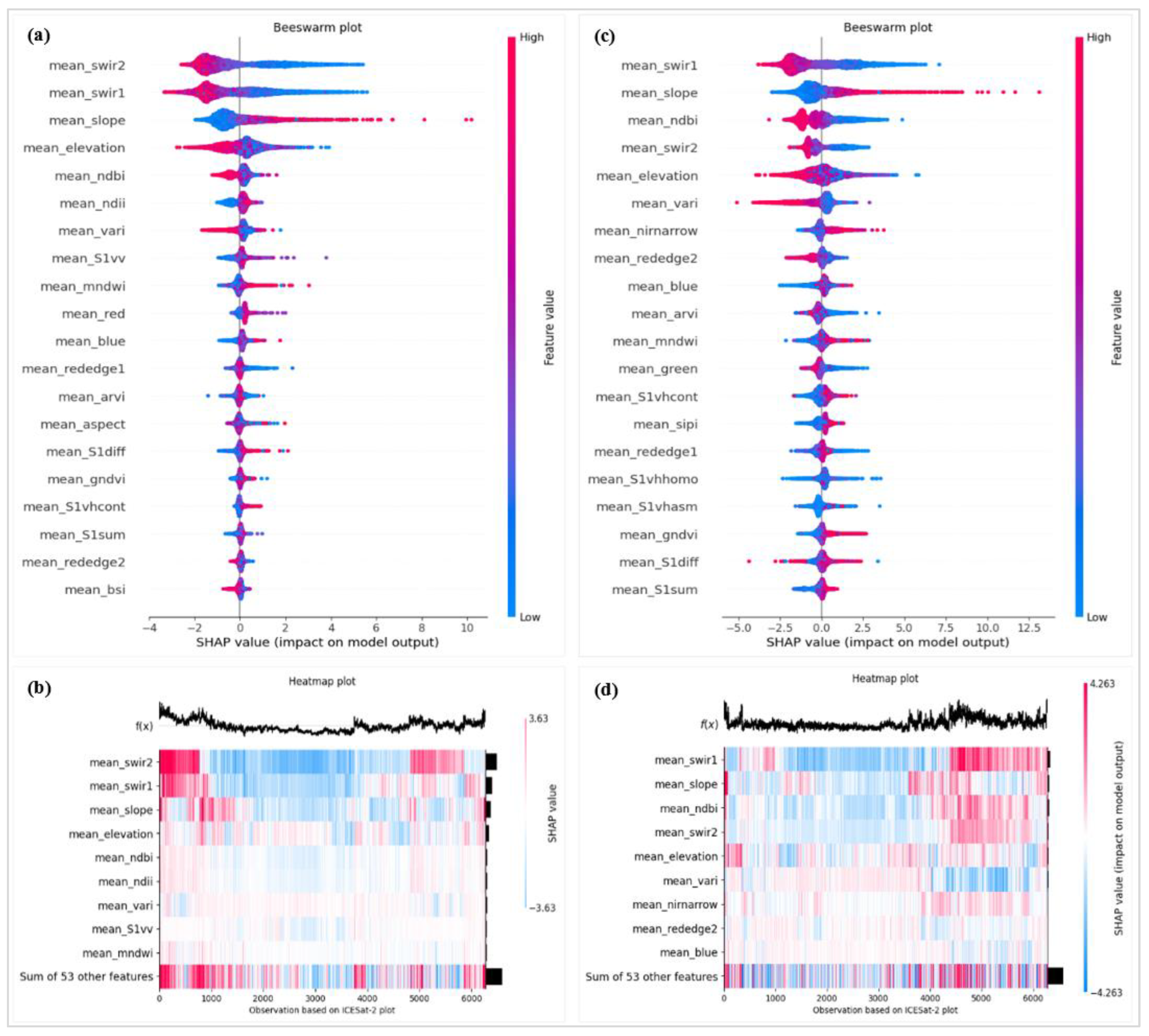
Over the course of modelling, the SHAP method allowed us to select about 20 predictors that exerted the strongest effects on model performance. Indeed, the importance of these features in estimating canopy height was further evaluated. For example, Figure 7 depicts the results for RF and XGBoost algorithms.
Fourteen importance features were common to the two algorithms. Yet, in the absence of unique features, those features that were shared by RF and XGBoost were very consistent in their respective rankings (W = 0.953, c2r = 24.77, df = 13, p = 0.025). Similar depictions of feature importance in the development of the remaining models (SVM, DNN) using SHAP are presented in Figure A2 (Appendix C).
3.3. Modelling Canopy Height Using ICESat-2 Data
Variables selected during the preliminary modelling stage and RF algorithm that resulted in remarkable performances allowed us to obtain the following results. It must be emphasized that only footprints containing more than 50 photons were considered to ensure that representative data were analyzed. Ultimately, 9781 ICESat-2 footprints were distributed in two groups of height classes that were defined in Section 2.6. Slightly higher metrics were obtained with Group 2 (r = 0.58; RMSE = 5.33; MAE = 3.92), compared to Group 1 (r = 0.51; RMSE = 5.46; MAE = 4.05).
Subsequent use of AutoML TPOT (see Section 2.6.2) made it possible to optimize the learning architecture by intelligently exploring thousands of pipelines (i.e., processing chains from preprocessing to modelling). This exploration made it possible to find the appropriate pipeline and automatically choose the appropriate hyperparameters for the model that best suited our data. The processing chain that led to these results is represented in Figure 8.
TPOT contributed to an improved performance of the canopy height prediction model that was developed. We refer to this model as rf_icesat-2_rh98, a designation that refers to the RF algorithm, ICESat-2 data and RH98 from which it was developed. The metrics obtained with this model are: r = 0.65; RMSE = 5.10; and MAE = 3.80. The regression curve, indicating the dispersion of heights extracted from ICESat-2 compared to predicted values, is shown in Figure 9. An initial observation of the distribution of predictions on this graph compared with the 1:1 line shows that the model tends to overestimate small canopies (< 10 m), to correctly estimate medium canopy heights ([10 m -20 m]) and to underestimate large canopies (> 20 m).
AutoGluon was applied to improve modelling performance. Given that it is a very complex ML system, AutoGluon is computationally very intensive, resource-intensive, difficult to debug and may make inappropriate assumptions regarding both parameters and data types [95,96,58]. The results that we subsequently obtained (r = 0.64; RMSE = 5.12; MAE = 3.83) were slightly higher than those of a simple RF (see Table 5), yet they remain very close to those obtained with TPOT.
3.4. Modelling Canopy Height from GEDI Data
The same tools and methods that were used with the ICESat-2 data to inform the choice of hyper-parameters and selection of variables with strong contributions to modelling were applied to predictions from the GEDI data. Table 7 summarizes performance metrics for nine configurations of canopy prediction models defined during data filtering (Section 2.5.2) and developed from GEDI.
Table 7 presents a heatmap of accuracy metrics for 63 prediction models that had been established, with seven relative heights under the nine configurations (see Section 2.5.2). For reference purposes, these models are designated as rf_gedi_configx_rhy, i.e., the model that was established with the Random Forest algorithm, based on GEDI data in configuration x with relative height y, (where x is the configuration number ranging from 1 to 9, and y is the percentage of relative height increasing from 75 to 100% in 5% increments. Through use of the simple RF algorithm and considering only Pearson coefficients, the rf_gedi_config9_rh98 model attained relatively high performance (r = 0.80), compared to the other models.
The heatmaps that were created for Pearson’s r, RMSE and MAE metrics exhibit similar overall trends, i.e., Configuration 9 emerges as the best performer, while Configurations 6, 2 and 1 are the worst. The remaining configurations are intermediate between the two extremes. In ranking correlations across configurations (columns) for each relative height category (rows) and subsequently determining their consistency, we found strong concordance among relative heights for Pearson’s correlations (Table 7). Visual assessments of r colour-ratings were consistent with rank ordering of the RF configurations. Strong ordering from worst to best performance was likewise noted for RMSE (ranked from highest to lowest error). MAE ranks (highest to lowest error) were also very consistent. Despite high levels of concordance, rank ordering was not identical among the performance metrics, given that error estimates also appeared to increase with increasing relative height percentiles, particularly for the worst performance scenarios (Table 7).
It should be noted that results of modelling with the RF algorithm from RH98 in group 1 (r = 0.73; RMSE = 4.95; MAE = 3.65) and in group 2 (r = 0.74; RMSE = 4.93; MAE = 3.66) also remain lower than those obtained for the GEDI data without the height classes. With the use of AutoML TPOT, the optimization of hyperparameters allowed us to produce a model with much higher performance (r = 0.84; RMSE = 4.15; MAE = 2.36) that was based on RF. The processing chain that yielded better results is represented in Figure 10.
In total, 28478 GEDI footprints that met the filtering criteria of Configuration 9 produced the more efficient model rf_gedi_config9_rh98. The regression curve in Figure 11 indicates strong dispersion of GEDI-based relative heights compared to the predicted values. Here again, according to the distribution of predictions in relation to the 1:1 line, it can be seen that the model slightly overestimates small canopies (< 10 m), makes a relatively better estimate of medium canopy heights ([10m -25 m]) and underestimates larger canopies (> 25 m). But this distribution is much more aligned or oriented more closely with the 1:1 line than does the scatterplot depicted in Figure 9.
Application of AutoML AutoGluon to the GEDI data resulted in a model with good performance (r = 0.83; RMSE = 4.16; MAE = 2.65) compared to using the RF algorithm alone. The results are comparable to those obtained with Auto-ML TPOT. Table 8 shows the effects of using Auto-ML TPOT and AutoGluon in improving the performance of models developed with both types of satellite LiDAR data compared to models developed simply with the RF algorithm.
Both sources of data showed consistent improvement in performance metrics with the application of AutoGluon to the RF model, which was then followed by an improvement with TPOT, with progressively increasing r and progressively decreasing error values with each improvement (W = 0.975, c2r = 14.62, df = 5, p = 0.012). Mean (± SD) Pearson coefficient for GEDI was 0.823 (± 0.021), while that of ICESat-2 was 0.633 (± 0.021). RMSE and MAE estimates were consistently lower for GEDI compared to ICESat-2. The three performance metrics obviously differed between the two datasets, significantly so (1-df directed contrast: Z = 11.57). The application of AutoGluon produced metrics that were slightly lower than those obtained with TPOT, which exhibited the best performance. We then continued analyses of the results of this study with the models developed using the TPOT method.
3.5. Forest Canopy Height Mapping from Developed Models
3.5.1. Forest Canopy Height Map Created from the ICESat-2 Based Model
The rf_icesat-2_rh98 is the model that was selected from the analysis of the ICESat-2 data. It was used to produce the continuous canopy height map of the study area at a spatial resolution of 30 m. The map encompassing Ecological zone 4 is presented in Figure 12.
Regarding the performance of the model used to produce this map, the predicted minimum and maximum canopy heights are respectively 4.20 m and 38.75 m, while predicted mean height (± SD) is 14.26 m (± 4.24 m). Figure 12 contains two zoom rectangles at different scales (Fig. 12b and Fig 12c), which present patterns that were very similar to those that are observed in high-resolution Google Earth images corresponding to the extents of these zooms (Figs. 12d and 12e, respectively).
3.5.2. Forest Canopy Height Map from GEDI-Based Model
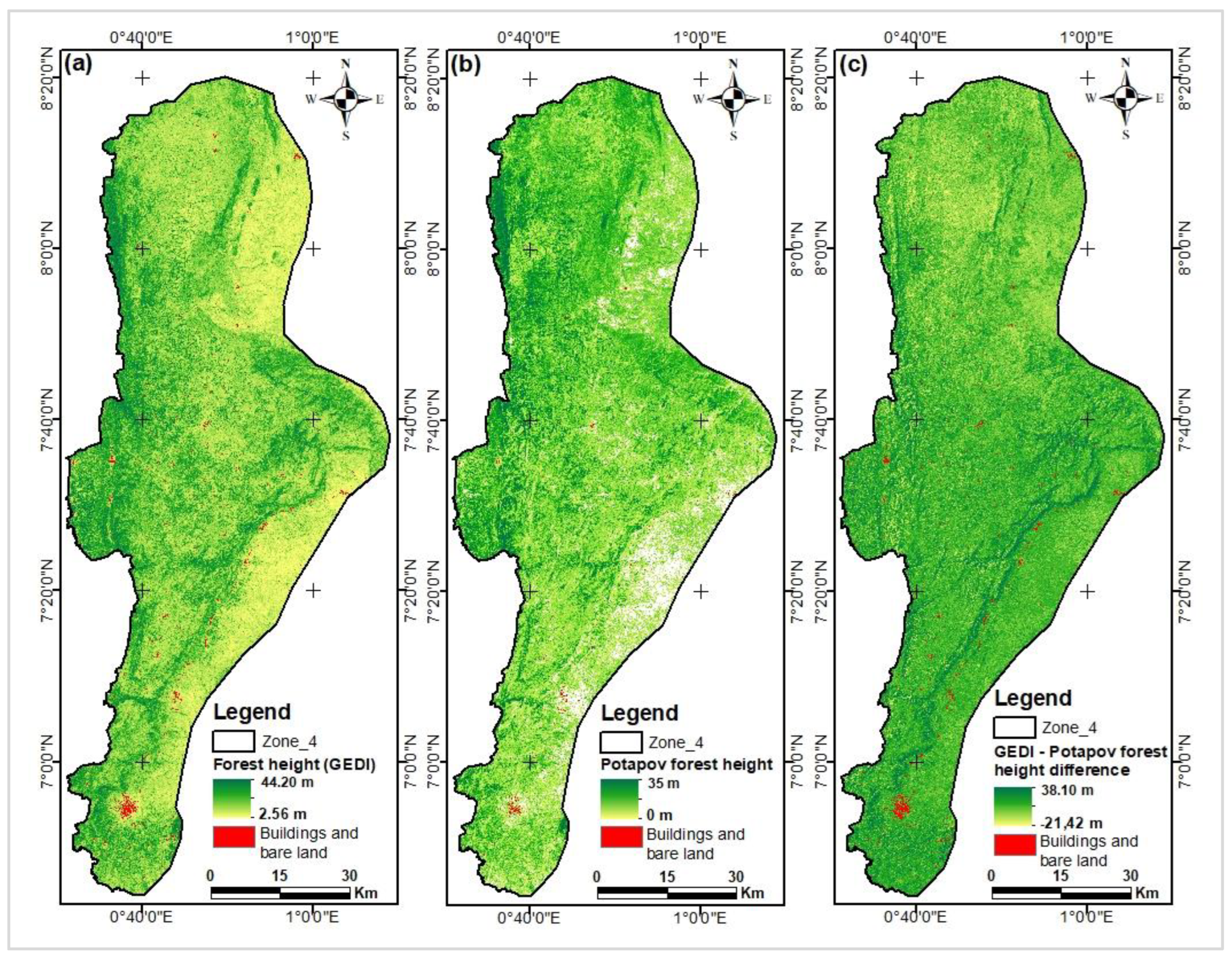
After all analyses were completed and improvements were made to the developed models (see Section 3.4), the rf_gedi_config9_rh98 model was retained for the GEDI data. It was used to produce a continuous canopy height map of the study area at a spatial resolution of 30 m. This map is presented in Figure 13 and follows the same format as Figure 12.
This continuous map is likewise the result of predicting canopy height using the model that learned best from GEDI (spatially discontinuous) data, relying upon a combination of continuous multisource variables, which provided the most accurate results when developing the model. Given the performance of the model used to produce this map, predicted minimum and maximum canopy heights are respectively 2.56 m and 44.20 m, while mean (± SD) height is 11.23 m (± 5.17 m). Figure 13 contains two zooms at different scales (Figs. 13b and 13c), which also show patterns almost similar to their corresponding high-resolution Google Earth images for the same footprints (Figs. 13d and 13e).
3.6. Comparative Analysis of Developed Models with Existing Products
No similar products exist for comparable studies that have been conducted locally in our study area to which our results could be compared. Regression was conducted on the field data collected from the ICESat-2 footprints, and those values predicted from these same plots made it possible to validate the model that was developed with these data (r = 0.54; RMSE = 3.11; MAE = 2.54). Given that we did not have field data for footprints of the GEDI products to which we could compare predictions of the optimal model established from these data, we used relative heights derived from data collected in the second National Forest Inventory (IFN2) to perform a similar regression. The only maps of canopy height available for the area are global maps that had been created by Lang et al. [97] and Potapov et al. [10]. From these maps, canopy heights were extracted from footprints of the ICESat-2, GEDI and IFN2 plots to compare them with their predicted values. Various linear regressions conducted with these data made it possible to estimate correlations between the extracted or existing data and their predicted values (Table 9). For the sake of simplicity, we refer to Lang et al. [97] and Potapov et al. [10] as “Lang" and "Potapov," respectively, in the following tables and figures, and in their canopy height mapping products.
This table shows that the predictions of canopy height made with the model based on data extracted from ICESat-2 are more closely correlated with those of the Lang map (r = 0.71, RMSE = 3.38, MAE = 2.55) than they are with those of Potapov (r = 0.62, RMSE= 3.80, MAE = 2.93). Similarly, predictions of canopy height using the model based on data extracted from GEDI are more consistent with Lang's map (r = 0.65, RMSE = 5.50, MAE = 4.17) than with Potapov's (r = 0.55, RMSE= 6.04, MAE = 4.64). On the other hand, the heights measured during NFI2 are closer to the canopy height estimates of the model based on data extracted from GEDI (r = 0.63, RMSE= 3.40, MAE = 2.65), than they are to those predicted with the model based on ICESat-2 (r = 0.55, RMSE = 3.65, MAE = 2.98).
In order to better compare the canopy height maps produced during this study, both with each other and with those of other authors, most notably Lang and Potapov, we performed image subtractions and then analyzed the results. Histograms of the maps resulting from the models developed by this study and those of their differences are presented in this section. Those maps resulting from the subtraction between the GEDI-based map and those of Lang and Potapov are presented and analyzed in the Discussion (see Section 4.3). Figure 14 presents the histograms of the GEDI-based map, the ICESat-2-based map and the map resulting from differences between these two maps.
The analysis of the histogram of the map that is based on GEDI (Figure 14a) reveals that more than 300 000 pixels have heights less than 5 m, while ICESat-2 (Figure 14b) shows less than 50 000 pixels in that range. This implies that the prediction model based on GEDI is much more sensitive to shorter canopies compared to that of ICESat-2. This response is also observed in the histogram of the resulting difference map (Figure 14c), which indicates most pixels are negative. The analysis of this last histogram further reveals that the model developed from ICESat-2 data overestimates heights most of the time, compared to that developed from GEDI data. Nevertheless, the average of the deviations is relatively small, and it should be noted in this histogram (Figure 14c) that the curve of the normal distribution is completely flattened in the tails, tending towards 0. This means that pixels with large positive or negative deviations are very few and that the source maps from which these difference maps are derived are relatively close to one another. The maps relating to these different image subtractions can be consulted in Figure A3, Figure A4, and Figure A5 in Appendix D, while the related discussions are presented in session 4.3.
4. Discussions
4.1. Performance of Multisource Satellite Variables in Estimating Forest Height
In this study, variables from optical, radar and topographic data were integrated with ICESat-2 and GEDI satellite LiDAR data. These combinations were used to develop models for estimating canopy height of forest-savanna mosaics in the Sudano-Guinean zone of West Africa. The importance of these variables in contributing to model development depends upon the method that is used for the assessment, and the algorithm that is used for this purpose. For example, Figure 7 reveals that in predicting responses with the RF model (Figure 7a), the ten most important covariates (in order) are swir2, swir1, slope, elevation, ndbi, ndii, vari, s1vv, mndwi and blue bands. In contrast, predictions made with the XGBoost model (Figure 7b) consisted (in order) of 10 covariates: swir1, slope, ndbi, swir2, elevation, vari, nirnarrow, rededge2, blue and arvi.
From literature reports, it is generally accepted that radar data would exhibit increased sensitivity to the vertical structure of the forest and the variables derived from them would allow for perfect estimation of the parameters of forest vertical structure, including canopy height [97,98,99] . Contrary to this assertion, which is widely accepted by several other studies, our results illustrated in Figure 6 indicate a strong contribution of variables from optical and topographic data sources to canopy height estimation, while those derived from radar data contribute very little. Our finding is consistent with Xi et al. [17], who also noted that vegetation indices and topographic information from Sentinel-2 and SRTM optical data respectively contributed much more effectively to the establishment of canopy height prediction models compared to texture measurements and backscatter variables from Sentinel-1 radar data. This result of our research is supported by the study by Luo et al. [100], who concluded that Sentinel-2-derived variables significantly contributed to the canopy height estimation model, unlike backscatter coefficients and textural parameters derived from Sentinel-1. In future studies, further investigations of contributions of variables by source would be relevant, together with the effects of their combinations in estimating forest structural parameters, particularly in complex tropical ecosystems of forest-savannah mosaics.
4.2. Comparative Analysis of ICESat-2 and GEDI Data Performance
In combination with multi-spectral, radar and topographic data, ICESat-2 and GEDI data have made it possible to develop models for predicting canopy height. The metrics of the best model that was established from ICESat-2 data are: r = 0.65; RMSE = 5.10 m; and MAE = 3.80 m. In contrast, metrics of the model established with GEDI data appear to be much improved (r = 0.84; RMSE = 4.15 m; MAE = 2.36 m). Therefore, GEDI emerges as providing better estimates of heights compared to ICESat-2. Moreover, these different results had been obtained by considering relative height RH98. Furthermore, the in situ heights measured during NFI2 national inventory are more consistent with the canopy heights estimated by the GEDI model (r = 0.63; RMSE = 3.40; MAE = 2.65) than with those estimated by the ICESat-2 model (r = 0.55; RMSE = 3.65; MAE = 2.98). The superiority of GEDI over ICESat-2 has been reported in previous work in other regions. This is the case, for example, of Zhu et al. [9], whose models with relative height RH98 obtained RMSE error parameters ranging from 3.61 m to 4.23 m with GEDI data, and from 4.76 m to 10.23 m with ICESat-2. The performance superiority of GEDI versus ICESat-2 is consistent with several other literature reports, including those of Liu et al. [13], Liu et al. [58] and Zhu et al. [101], who likewise had reported better estimates with GEDI.
One possible reason for this response is that relative heights contained in the ICESat-2 data, each representing an average value over 100 m, consist of several laser pulses that are spaced 0.7 m apart (Figure 3a) and, thus, contain a certain level of imprecision. What results in a low level of correlation of tree heights with ground surface data collected in their footprints. The other reason is that the GEDI data, when acquired, are more densely sampled than the ICESat-2 data and have individual and direct ground footprints of their emitted laser beams (Figure 3b). In this study, the ground data were collected in the footprints of the ICESat-2 data only. This does not permit direct validation of the estimates that are made using GEDI data. Collection of ground data in GEDI footprints, therefore, would be of great importance for future work in our study area, or more generally, in forest-savannah mosaics.
4.3. Comparison of Map Products with Similar Recent Work
To properly compare the cartographic products of this study with existing ones, we established histograms from the maps resulting from the differences between the GEDI-based map and that of Lang on the one hand, and the GEDI-based map and that of Potapov on the other hand. Given that these two researchers did not use the ICESat-2 data, this comparison could only be done with our GEDI-based model. Figure 15 below presents the distribution of these differences in canopy heights between these products.
It is evident from Figure 15a that the mean of the deviations is negative, which could mean that the Lang model overestimates some canopy heights compared to our GEDI-based model. This is opposite to the phenomenon in Figure 15b, in which the histogram exhibits a positive mean of the deviations. The Potapov model, therefore, underestimates some canopy heights compared to our model. In this situation, where the models of the two researchers appear to overestimate or underestimate canopy height compared to our model, could be related to differences in algorithms that are used by each of these studies regarding the development of these models. Indeed, while we used the RF algorithm, Lang et al. [97] considered a probabilistic deep-learning approach based upon an ensemble of deep convolutional neural networks (CNNs), while Potapov et al. [10] employed a machine-learning algorithm based on an ensemble of bagging regression trees. In this case, it would be interesting for future studies to further investigate effects of the choice of algorithms on the quality of the developed models. .
The standard deviation of the difference map between the GEDI model versus Lang appears to be lower than that depicted in the difference map between the GEDI model versus Potapov. This implies that the distribution of these deviations is much more tightly grouped about their mean in the first case, while in the second case, these deviations are more dispersed and relatively far from their mean. This observation indicates that the GEDI-based model of this study would be closer to that of Lang than to Potapov. Nevertheless, the mean of the deviations is relatively low, and we also note that in these two histograms, the curve of the normal distribution is completely flattened in the tails, tending towards 0. Furthermore, the number of pixels with large positive or negative deviations is quite limited and would be more likely linked to an edge-effect of the images. As in the case of Figure 14c, the source maps from which each of these difference maps were derived are therefore relatively close to each other.
4.4. Important Factors and Limitations in Estimating Canopy Height
Histogram analysis had demonstrated that the more sensitive the model is to shorter vegetation, the better it would be able to correctly estimate the canopy heights of our study area. Our study area consists of forest-savannah mosaics, which are ecosystems with mostly small and often scattered trees. In these ecosystems, the GEDI-based model therefore performed better than the ICESat-2-based model, given its ability to better estimate the heights of both tall and short canopies. This performance would also be linked to the high density of GEDI footprints compared to ICESat-2. Similar canopy height estimation studies by Liu et al. [58] in China, Zhu et al. [9] in the United States, and Sothe et al. [57] in Canada have shown remarkable performance, partly due to the continuity and homogeneity of the forest landscape in which their models were applied. Therefore, further investigation is warranted regarding the effect of different ecosystems and forest types on performance levels of canopy height estimation models developed from GEDI and ICESat-2 data, especially in forest-savannah mosaics of the Sudano-Guinean zone.
Furthermore, the choice of the dependent variable in such predictions greatly influences the accuracies of the models that are being developed. In this study, we evaluated the relative heights that were extracted from satellite LiDAR data before selecting RH98 as the optimal dependent variable in model development. Our results from regressions used to assess correlations between extracted or existing data and predicted values (Table 9) also indicate that the choice of a prediction parameter is very critical to the modelling process. Indeed, Lang et al. [97] likewise used RH98 as a dependent variable, while Potapov et al. [10] used RH95. The NFI2 data were slightly further away from the canopy heights extracted from the Potopov map (r = 0.46; RMSE = 4.21; MAE = 3.28), but closer to the canopy heights extracted from the Lang map (r = 0.64; RMSE = 3.96; MAE = 3.09), which are most similar to our own (r = 0.63; RMSE = 3.40; MAE = 2.65). Therefore, our study joins those of Lang et al. ([97]) and Ngo et al. [102], as well as many others, in confirming that RH98 would be the most appropriate RH to be used in best estimates of canopy height based upon GEDI data.
Ultimately, the development of canopy height prediction models from satellite LiDAR data is strongly dependent upon several parameters. In order to optimize the parameters that would make these models more accurate and geographically adapted, the spatio-temporal coherence of the independent covariates that are used must be taken into account, together with the characteristics of the ecosystems to which these models are being applied, and the algorithms or learning models that are used. To the best of our knowledge, such studies involving the combination of optical, radar, topographic and satellite LiDAR data to develop models for estimating canopy heights in the forest-savanna mosaics of the Sudano-Guinean zone did not exist prior to ours. Taking into account the elements of discussions and perspectives of this study would help improve the quality of canopy height or forest biomass models in future studies.
5. Conclusions
In our search for greater accuracy in estimating the canopy height of forest-savannah mosaics in the Sudano-Guinean zone, the research relied upon a combination of multisource and multisensor data. Four machine-learning algorithms (RF, SVM, XGBoost, DNN) were evaluated before selecting Random Forest, which was demonstrably more efficient in predicting canopy height across the study area than the remaining models. Our results indicate that the final model developed from GEDI data is more efficient than that derived from ICESat-2. Investigations carried out during this research also reveal that the prediction models based on grouping data by height classes did not provide any improvement compared to those where the height classes were not defined, using both GEDI and ICESat-2 data.
Estimation of canopy height was best achieved using combinations of several types of remote sensing data rather than using each one in isolation. Yet, we found that variables derived from optical and topographic data contributed much more to the development of better performing models that did those derived from radar data, which showed very little sensitivity. Furthermore, future studies should be able to assess the effects of different variables extracted from the radar data for the estimation of forest and vegetation structural parameters. The return signal that is received by satellite LiDAR sensors depends upon the characteristics of the land cover (height, density, canopy closure). Future studies, therefore, could also analyze the effects of ecosystem characteristics on the quality of GEDI-based models, especially in the ecosystems within our study area, which are characterized by sparse and relatively small vegetation types or patches.
In the short-term, our results of canopy height modelling could be used by local decision-makers for forest management in the study area by favouring the use of GEDI data in estimating canopy height. In the long-term, the estimation of field dendrometric parameters within GEDI data footprints is more necessary than ever in order to better validate the models that have been developed. Validation of these GEDI data and models in this particular eco-climatic zone would also provide forest managers with an appropriate tool for estimating aboveground biomass to better understand forest dynamics and carbon fluxes and, thus, adapt their practices and management methods to the requirements of REDD+.
Author Contributions
Conceptualization: A.K., K.G.; Methodology: A.K., K.G.; Data collection: A.K.; Data processing: A.K., K.G., G.A.F.K.; Modelling: A.K., G.A.F.K.; Preparation of the initial draft: A.K.; Supervision: K.G.; Revision & Editing: A.K., K.G., G.A.F.K.
Funding
This research was funded by Programme Canadien de Bourse de la Francophonie, through Global Affairs Canada (Government of Canada), under project number P-008649, as well as the Natural Sciences and Engineering Research Council of Canada (NSERC Discovery grants RGPIN-2018-06101, RGPIN-2024-05199, and NSERC CREATE 543360-2020).
Declaration of data availability
The data are available and can be obtained by contacting the first author.
Acknowledgments
We thank all authors and reviewers for their guidance and contributions to the writing of this manuscript. We also thank students of the INFA (Tové), together with staff of the Laboratory of Botany and Plant Ecology (Faculty of Sciences, University of Lomé), for their invaluable assistance during the collection of the field data. W.F.J. Parsons translated the manuscript into English.
Conflicts of Interest
The authors declare no conflicts of interest. The funder had no role in the study design, data collection, analysis, interpretation, writing of the manuscript, or in the decision to publish the results.
Appendix A
Figure A1.
Figure A1.
Elevation of the soil surface (a) and the canopy surface (b), and photon returns.
Appendix B
Table A1.

Table A1.
List of covariables used in this study.
| No. | Feature Abbrev. | Description | Native Band / Formula | References |
|---|---|---|---|---|
| 1 | S1vv | Vertical transmit-vertical channel backscattering coefficients, dB | VV | [103] |
| 2 | S1vh | Vertical transmit-horizontal channel backscattering coefficients, dB | VH | [103] |
| 3 | S1diff | Bands difference between VV and VH | [104] | |
| 4 | S1mdpsvi | Modified Dual Polarimetric Sar Vegetation Index | [105] | |
| 5 | S1npdi | Normalized Polarization Difference Index | [106] | |
| 6 | S1prod | Bands product between VV and VH | [104] | |
| 7 | S1rept | Bands report between VV and VH | [16] | |
| 8 | S1rvi | Ratio Vegetation Index | 4*VH/(VV+VH) | [104] |
| 9 | S1sum | Bands sum between VV and VH | [107] | |
| 10 | S1vhasm | VH GLCM* Angular Second Moment | [108] | |
| 11 | S1vhcont | VH GLCM Contrast | [108] | |
| 12 | S1vhcorr | VH GLCM Correlation | [108] | |
| 13 | S1vhdiss | VH GLCM Dissimilarity | [108] | |
| 14 | S1vhener | VH GLCM Energy | [108] | |
| 15 | S1vhent | VH GLCM Entropy | [108] | |
| 16 | S1vhhomo | VH GLCM Homogeneity | [108] | |
| 17 | S1vhmax | VH GLCM Maximum | [108] | |
| 18 | S1vhmean | VH GLCM Mean | [108] | |
| 19 | S1vhvar | VH GLCM Variance | [108] | |
| 20 | S1vvasm | VV GLCM Angular Second Moment | [108] | |
| 21 | S1vvcont | VV GLCM Contrast | [108] | |
| 22 | S1vvcorr | VV GLCM Correlation | [108] | |
| 23 | S1vvdiss | VV GLCM Dissimilarity | [108] | |
| 24 | S1vvener | VV GLCM Energy | [108] | |
| 25 | S1vvent | VV GLCM Entropy | [108] | |
| 26 | S1vvhomo | VV GLCM Homogeneity | [108] | |
| 27 | S1vvmax | VV GLCM Maximum | [108] | |
| 28 | S1vvmean | VV GLCM Mean | [108] | |
| 29 | S1vvvar | VV GLCM Variance | [108] | |
| 30 | blue | Blue band | B2 | [109] |
| 31 | green | Green band | B3 | [109] |
| 32 | red | Red band | B4 | [109] |
| 33 | rededge1 | Red edge1 band | B5 | [109] |
| 34 | rededge2 | Red edge2 band | B6 | [109] |
| 35 | rededge3 | Red edge3 band | B7 | [109] |
| 36 | nir | Near-infrared (NIR) band | B8 | [109] |
| 37 | nirnarrow | Near-infrared narrow (NIR-narrow) band | B8A | [109] |
| 38 | wir1 | Short-wave infrared (SWIR1) band | B11 | [109] |
| 39 | swir2 | Short-wave infrared (SWIR 2) band | B12 | [109] |
| 40 | arvi | Atmospherically Resistant Vegetation Index | NIR − (2 × Red − Blue)/NIR+(2 × Red − Blue) | [110] |
| 41 | bsi | Bare Soil Index | [111] | |
| 42 | evi | Enhanced Vegetation Index | 2.5 × (NIR − Red)/(NIR + 6Red − 7.5 × Blue + 1) | [110] |
| 43 | gndvi | Green Normalized Difference Vegetation Index | (NIR - Green)/(NIR + Green) | [16] |
| 44 | mndwi | Modified Normalized Difference Water Index | (Green – SWIR) / (Green + SWIR) | [112] |
| 45 | msavi | Modified Soil Adjusted Vegetation Index | [113] | |
| 46 | mtvi | Modified Triangular Vegetation Index | 1.2*[1.2(NIR - Green) - 2.5*(Red - Green)] | [114] |
| 47 | ndbi | Normalized Difference Built-up Index | [115] | |
| 48 | ndii | Normalized Difference Infrared Index | [116] | |
| 49 | ndvi | Normalized Difference Vegetation Index | (NIR − Red) / (NIR + Red) | [110] |
| 50 | osavi | Optimized Soil Adjusted Vegetation Index | [117] | |
| 51 | rdvi | Renormalized Difference Vegetation Index | [118] | |
| 52 | rvi | Ratio Vegetation Index | (Red /NIR) | [119] |
| 53 | savi | Soil Adjusted Vegetation Index | 1.5 x (NIR - Red)/(NIR + Red + 0.5) | [120] |
| 54 | sipi | Structure Insensitive Pigment Index | (NIR – Blue) / (NIR – Red) | [114] |
| 55 | sr | Simple Ratio | (NIR/ Red) | [121] |
| 56 | vari | Visible Atmospherically Resistant Index | (Green − Red)/(Green + Red − Blue) | [122] |
| 57 | vsi | Vegetation Structure Index | NDVI/(1-NIR) | [123] |
| 58 | aspect | Aspect | [124] | |
| 59 | elevation | Elevation | [124] | |
| 60 | slope | Slope | [124] |
*GLCM: Grey-Level Co-occurrence Matrix.
Appendix C
Figure A2.
Figure A2.
Determining the importance of variables using the SHAP method: Beeswarm (a & c) and Heatmap (b & d) plots for the Random Forest (a & b) and XGBoost (c & d) models.
Figure A2.
Determining the importance of variables using the SHAP method: Beeswarm (a & c) and Heatmap (b & d) plots for the Random Forest (a & b) and XGBoost (c & d) models.
Appendix D
Figures A3, A4 and A5: Difference between Canopy Height Maps by Subtraction
Figure A3.
Map of canopy height based on ICESat-2 (a) and that based on GEDI (b), and the difference between them (GEDI - ICESat-2) (c).
Figure A3.
Map of canopy height based on ICESat-2 (a) and that based on GEDI (b), and the difference between them (GEDI - ICESat-2) (c).
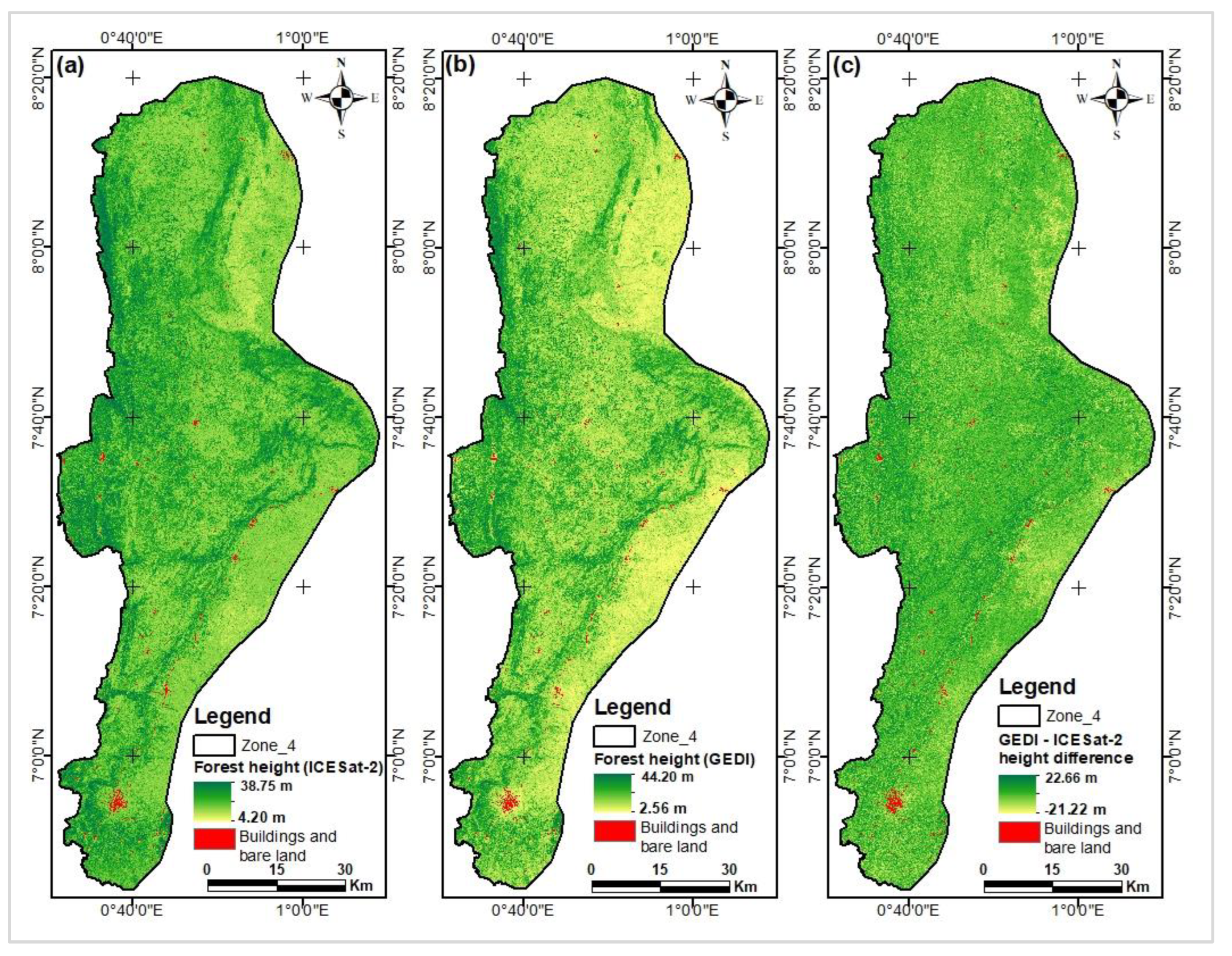
Figure A4.
Map of canopy heights based on GEDI (a) and Lang (b), and their difference (GEDI - Lang) (c).
Figure A4.
Map of canopy heights based on GEDI (a) and Lang (b), and their difference (GEDI - Lang) (c).
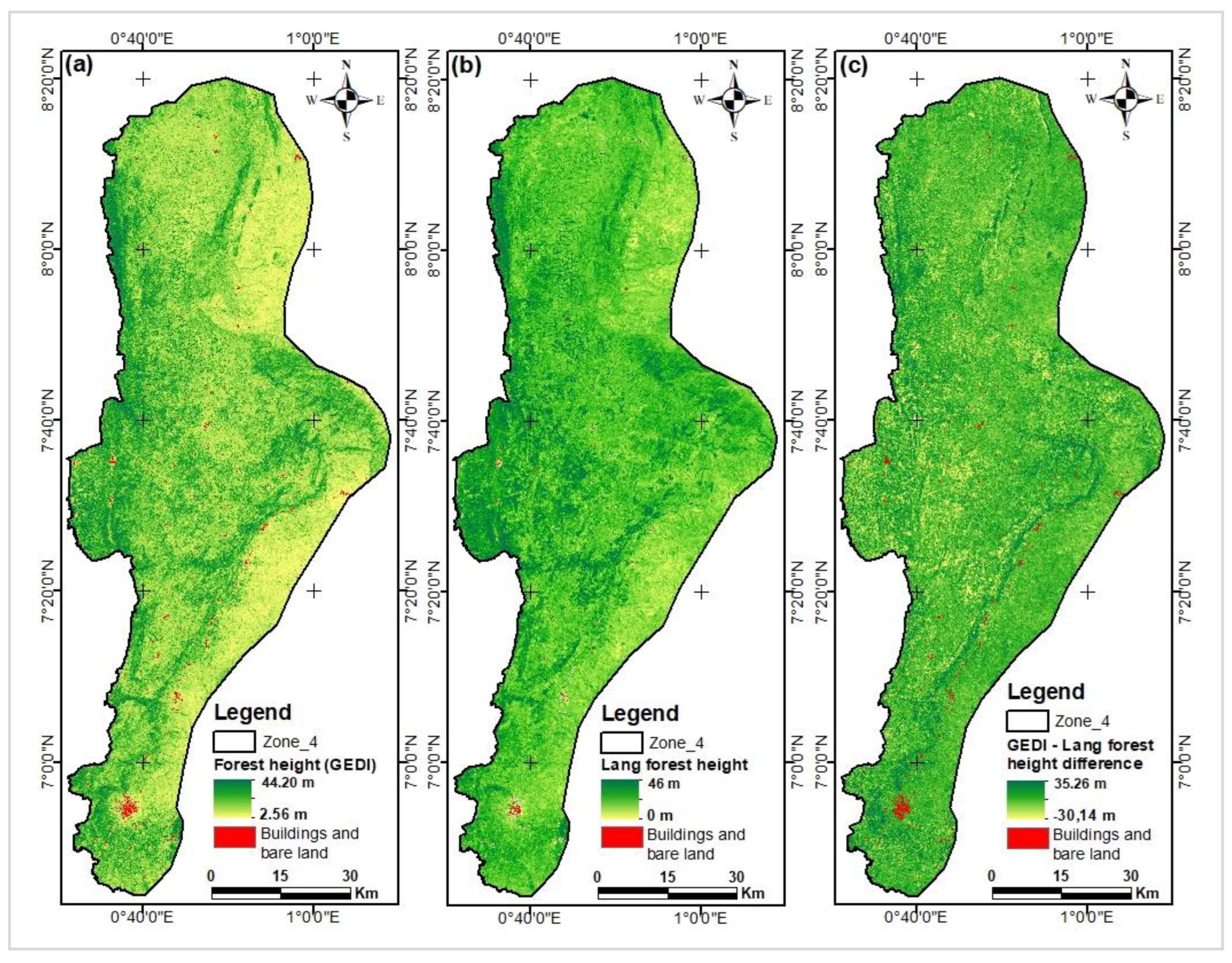
Figure A5.
Map of canopy heights based on GEDI (a) and Potapov (b), and their difference (GEDI - Potapov) (c).
Figure A5.
Map of canopy heights based on GEDI (a) and Potapov (b), and their difference (GEDI - Potapov) (c).
References
- Van Houtan, K.S.; Tanaka, K.R.; Gagné, T.O.; Becker, S.L. The Geographic Disparity of Historical Greenhouse Emissions and Projected Climate Change. Science Advances 2021, 7, eabe4342. [CrossRef]
- Xu, X.; Huang, A.; Belle, E.; De Frenne, P.; Jia, G. Protected Areas Provide Thermal Buffer against Climate Change. Science Advances 2022, 8, eabo0119. [CrossRef]
- Moore, J.W.; Schindler, D.E. Getting Ahead of Climate Change for Ecological Adaptation and Resilience. Science 2022, 376, 1421–1426. [CrossRef]
- Babiker, M.; Berndes, G.; Blok, K.; Cohen, B.; Cowie, A.; Geden, O.; Ginzburg, V.; Leip, A.; Smith, P.; Sugiyama, M.; et al. Cross-Sectoral Perspectives (Chapter 12). In; Shukla, A.R., Skea, J., Slade, R., Al Khourdajie, A., van Diemen, R., McCollum, D., Pathak, M., Some, S., Vyas, P., Fradera, R., Belkacemi, M., Hasija, A., Lisboa, G., Luz, S., Malley, J., Eds.; Cambridge University Press: Cambridge, UK and New York, NY, USA, 2022; pp. 1245–1354 ISBN 978-1-00-915792-6.
- Fischer, H.W.; Chhatre, A.; Duddu, A.; Pradhan, N.; Agrawal, A. Community Forest Governance and Synergies among Carbon, Biodiversity and Livelihoods. Nat. Clim. Chang. 2023, 13, 1340–1347. [CrossRef]
- Lamb, W.F.; Gasser, T.; Roman-Cuesta, R.M.; Grassi, G.; Gidden, M.J.; Powis, C.M.; Geden, O.; Nemet, G.; Pratama, Y.; Riahi, K.; et al. The Carbon Dioxide Removal Gap. Nat. Clim. Chang. 2024, 14, 644–651. [CrossRef]
- Bonan, G.B. Forests and Climate Change: Forcings, Feedbacks, and the Climate Benefits of Forests. Science 2008, 320, 1444–1449. [CrossRef]
- Le Quéré, C.; Andrew, R.M.; Friedlingstein, P.; Sitch, S.; Pongratz, J.; Manning, A.C.; Korsbakken, J.I.; Peters, G.P.; Canadell, J.G.; Jackson, R.B.; et al. Global Carbon Budget 2017. Earth System Science Data 2018, 10, 405–448. [CrossRef]
- Zhu, X.; Nie, S.; Wang, C.; Xi, X.; Lao, J.; Li, D. Consistency Analysis of Forest Height Retrievals between GEDI and ICESat-2. Remote Sensing of Environment 2022, 281, 113244. [CrossRef]
- Potapov, P.; Li, X.; Hernandez-Serna, A.; Tyukavina, A.; Hansen, M.C.; Kommareddy, A.; Pickens, A.; Turubanova, S.; Tang, H.; Silva, C.E.; et al. Mapping Global Forest Canopy Height through Integration of GEDI and Landsat Data. Remote Sensing of Environment 2021, 253, 112165. [CrossRef]
- Herold, M.; Carter, S.; Avitabile, V.; Espejo, A.B.; Jonckheere, I.; Lucas, R.; McRoberts, R.E.; Næsset, E.; Nightingale, J.; Petersen, R.; et al. The Role and Need for Space-Based Forest Biomass-Related Measurements in Environmental Management and Policy. Surv Geophys 2019, 40, 757–778. [CrossRef]
- Chen, J.; Yan, F.; Lu, Q. Spatiotemporal Variation of Vegetation on the Qinghai–Tibet Plateau and the Influence of Climatic Factors and Human Activities on Vegetation Trend (2000–2019). Remote Sensing 2020, 12, 3150.
- Liu, A.; Cheng, X.; Chen, Z. Performance Evaluation of GEDI and ICESat-2 Laser Altimeter Data for Terrain and Canopy Height Retrievals. Remote Sensing of Environment 2021, 264, 112571. [CrossRef]
- Hurtt, G.; Zhao, M.; Sahajpal, R.; Armstrong, A.; Birdsey, R.; Campbell, E.; Dolan, K.; Dubayah, R.; Fisk, J.P.; Flanagan, S.; et al. Beyond MRV: High-Resolution Forest Carbon Modeling for Climate Mitigation Planning over Maryland, USA. Environ. Res. Lett. 2019, 14, 045013. [CrossRef]
- Li, W.; Niu, Z.; Shang, R.; Qin, Y.; Wang, L.; Chen, H. High-Resolution Mapping of Forest Canopy Height Using Machine Learning by Coupling ICESat-2 LiDAR with Sentinel-1, Sentinel-2 and Landsat-8 Data. International Journal of Applied Earth Observation and Geoinformation 2020, 92, 102163. [CrossRef]
- Zhang, N.; Chen, M.; Yang, F.; Yang, C.; Yang, P.; Gao, Y.; Shang, Y.; Peng, D. Forest Height Mapping Using Feature Selection and Machine Learning by Integrating Multi-Source Satellite Data in Baoding City, North China. Remote Sensing 2022, 14, 4434.
- Xi, Z.; Xu, H.; Xing, Y.; Gong, W.; Chen, G.; Yang, S. Forest Canopy Height Mapping by Synergizing ICESat-2, Sentinel-1, Sentinel-2 and Topographic Information Based on Machine Learning Methods. Remote Sensing 2022, 14, 364. [CrossRef]
- de Bem, P.P.; de Carvalho Junior, O.A.; Fontes Guimarães, R.; Trancoso Gomes, R.A. Change Detection of Deforestation in the Brazilian Amazon Using Landsat Data and Convolutional Neural Networks. Remote Sensing 2020, 12, 901. [CrossRef]
- Hemati, M.; Hasanlou, M.; Mahdianpari, M.; Mohammadimanesh, F. A Systematic Review of Landsat Data for Change Detection Applications: 50 Years of Monitoring the Earth. Remote Sensing 2021, 13, 2869. [CrossRef]
- Grabska, E.; Hostert, P.; Pflugmacher, D.; Ostapowicz, K. Forest Stand Species Mapping Using the Sentinel-2 Time Series. Remote Sensing 2019, 11, 1197. [CrossRef]
- Hemmerling, J.; Pflugmacher, D.; Hostert, P. Mapping Temperate Forest Tree Species Using Dense Sentinel-2 Time Series. Remote Sensing of Environment 2021, 267, 112743. [CrossRef]
- Nguyen, T.T.H.; Pham, T.A.; Luong, T.P. Estimate Tropical Forest Stand Volume Using SPOT 5 Satellite Image. IOP Conf. Ser.: Earth Environ. Sci. 2021, 652, 012016. [CrossRef]
- Peerbhay, K.; Adelabu, S.; Lottering, R.; Singh, L. Mapping Carbon Content in a Mountainous Grassland Using SPOT 5 Multispectral Imagery and Semi-Automated Machine Learning Ensemble Methods. Scientific African 2022, 17, e01344. [CrossRef]
- De Petris, S.; Sarvia, F.; Borgogno-Mondino, E. Uncertainties and Perspectives on Forest Height Estimates by Sentinel-1 Interferometry. Earth 2022, 3, 479–492. [CrossRef]
- Ge, S.; Su, W.; Gu, H.; Rauste, Y.; Praks, J.; Antropov, O. Improved LSTM Model for Boreal Forest Height Mapping Using Sentinel-1 Time Series. Remote Sensing 2022, 14, 5560. [CrossRef]
- Persson, H.; Fransson, J.E.S. Forest Variable Estimation Using Radargrammetric Processing of TerraSAR-X Images in Boreal Forests. Remote Sensing 2014, 6, 2084–2107. [CrossRef]
- Vastaranta, M.; Niemi, M.; Karjalainen, M.; Peuhkurinen, J.; Kankare, V.; Hyyppä, J.; Holopainen, M. Prediction of Forest Stand Attributes Using TerraSAR-X Stereo Imagery. Remote Sensing 2014, 6, 3227–3246. [CrossRef]
- Lei, Y.; Treuhaft, R.; Gonçalves, F. Automated Estimation of Forest Height and Underlying Topography over a Brazilian Tropical Forest with Single-Baseline Single-Polarization TanDEM-X SAR Interferometry. Remote Sensing of Environment 2021, 252, 112132. [CrossRef]
- Bao, J.; Zhu, N.; Chen, R.; Cui, B.; Li, W.; Yang, B. Estimation of Forest Height Using Google Earth Engine Machine Learning Combined with Single-Baseline TerraSAR-X/TanDEM-X and LiDAR. Forests 2023, 14, 1953. [CrossRef]
- Chen, W.; Zheng, Q.; Xiang, H.; Chen, X.; Sakai, T. Forest Canopy Height Estimation Using Polarimetric Interferometric Synthetic Aperture Radar (PolInSAR) Technology Based on Full-Polarized ALOS/PALSAR Data. Remote Sensing 2021, 13, 174. [CrossRef]
- Sa, R.; Nei, Y.; Fan, W. Combining Multi-Dimensional SAR Parameters to Improve RVoG Model for Coniferous Forest Height Inversion Using ALOS-2 Data. Remote Sensing 2023, 15, 1272. [CrossRef]
- Sinha, S.; Jeganathan, C.; Sharma, L.K.; Nathawat, M.S. A Review of Radar Remote Sensing for Biomass Estimation. Int. J. Environ. Sci. Technol. 2015, 12, 1779–1792. [CrossRef]
- Zhao, P.; Lu, D.; Wang, G.; Wu, C.; Huang, Y.; Yu, S. Examining Spectral Reflectance Saturation in Landsat Imagery and Corresponding Solutions to Improve Forest Aboveground Biomass Estimation. Remote Sensing 2016, 8, 469. [CrossRef]
- Naik, P.; Dalponte, M.; Bruzzone, L. Prediction of Forest Aboveground Biomass Using Multitemporal Multispectral Remote Sensing Data. Remote Sensing 2021, 13, 1282. [CrossRef]
- Ahmad, A.; Gilani, H.; Ahmad, S.R. Forest Aboveground Biomass Estimation and Mapping through High-Resolution Optical Satellite Imagery—A Literature Review. Forests 2021, 12, 914. [CrossRef]
- Gaveau, D.L.A.; Hill, R.A. Quantifying Canopy Height Underestimation by Laser Pulse Penetration in Small-Footprint Airborne Laser Scanning Data. Canadian Journal of Remote Sensing 2003, 29, 650–657. [CrossRef]
- Wilkes, P.; Jones, S.D.; Suarez, L.; Mellor, A.; Woodgate, W.; Soto-Berelov, M.; Haywood, A.; Skidmore, A.K. Mapping Forest Canopy Height Across Large Areas by Upscaling ALS Estimates with Freely Available Satellite Data. Remote Sensing 2015, 7, 12563–12587. [CrossRef]
- Liu, G.; Wang, J.; Dong, P.; Chen, Y.; Liu, Z. Estimating Individual Tree Height and Diameter at Breast Height (DBH) from Terrestrial Laser Scanning (TLS) Data at Plot Level. Forests 2018, 9, 398. [CrossRef]
- Tian, J.; Dai, T.; Li, H.; Liao, C.; Teng, W.; Hu, Q.; Ma, W.; Xu, Y. A Novel Tree Height Extraction Approach for Individual Trees by Combining TLS and UAV Image-Based Point Cloud Integration. Forests 2019, 10, 537. [CrossRef]
- Wulder, M.A.; White, J.C.; Nelson, R.F.; Næsset, E.; Ørka, H.O.; Coops, N.C.; Hilker, T.; Bater, C.W.; Gobakken, T. Lidar Sampling for Large-Area Forest Characterization: A Review. Remote Sensing of Environment 2012, 121, 196–209. [CrossRef]
- Esteban, J.; McRoberts, R.E.; Fernández-Landa, A.; Tomé, J.L.; Nӕsset, E. Estimating Forest Volume and Biomass and Their Changes Using Random Forests and Remotely Sensed Data. Remote Sensing 2019, 11, 1944. [CrossRef]
- Lang, N.; Schindler, K.; Wegner, J.D. Country-Wide High-Resolution Vegetation Height Mapping with Sentinel-2. Remote Sensing of Environment 2019, 233, 111347. [CrossRef]
- Morin, D.; Planells, M.; Baghdadi, N.; Bouvet, A.; Fayad, I.; Le Toan, T.; Mermoz, S.; Villard, L. Improving Heterogeneous Forest Height Maps by Integrating GEDI-Based Forest Height Information in a Multi-Sensor Mapping Process. Remote Sensing 2022, 14, 2079. [CrossRef]
- Simard, M.; Pinto, N.; Fisher, J.B.; Baccini, A. Mapping Forest Canopy Height Globally with Spaceborne Lidar. Journal of Geophysical Research: Biogeosciences 2011, 116. [CrossRef]
- Baghdadi, N.; le Maire, G.; Fayad, I.; Bailly, J.S.; Nouvellon, Y.; Lemos, C.; Hakamada, R. Testing Different Methods of Forest Height and Aboveground Biomass Estimations From ICESat/GLAS Data in Eucalyptus Plantations in Brazil. IEEE Journal of Selected Topics in Applied Earth Observations and Remote Sensing 2014, 7, 290–299. [CrossRef]
- Fayad, I.; Baghdadi, N.; Bailly, J.-S.; Barbier, N.; Gond, V.; Hajj, M.E.; Fabre, F.; Bourgine, B. Canopy Height Estimation in French Guiana with LiDAR ICESat/GLAS Data Using Principal Component Analysis and Random Forest Regressions. Remote Sensing 2014, 6, 11883–11914. [CrossRef]
- Narine, L.L.; Popescu, S.C.; Malambo, L. Synergy of ICESat-2 and Landsat for Mapping Forest Aboveground Biomass with Deep Learning. Remote Sensing 2019, 11, 1503. [CrossRef]
- Qi, W.; Lee, S.-K.; Hancock, S.; Luthcke, S.; Tang, H.; Armston, J.; Dubayah, R. Improved Forest Height Estimation by Fusion of Simulated GEDI Lidar Data and TanDEM-X InSAR Data. Remote Sensing of Environment 2019, 221, 621–634. [CrossRef]
- Tsao, A.; Nzewi, I.; Jayeoba, A.; Ayogu, U.; Lobell, D.B. Canopy Height Mapping for Plantations in Nigeria Using GEDI, Landsat, and Sentinel-2. Remote Sensing 2023, 15, 5162. [CrossRef]
- Alvites, C.; O’Sullivan, H.; Francini, S.; Marchetti, M.; Santopuoli, G.; Chirici, G.; Lasserre, B.; Marignani, M.; Bazzato, E. High-Resolution Canopy Height Mapping: Integrating NASA’s Global Ecosystem Dynamics Investigation (GEDI) with Multi-Source Remote Sensing Data. Remote Sensing 2024, 16, 1281. [CrossRef]
- Xing, Y.; Huang, J.; Gruen, A.; Qin, L. Assessing the Performance of ICESat-2/ATLAS Multi-Channel Photon Data for Estimating Ground Topography in Forested Terrain. Remote Sensing 2020, 12, 2084. [CrossRef]
- Lin, X.; Xu, M.; Cao, C.; Dang, Y.; Bashir, B.; Xie, B.; Huang, Z. Estimates of Forest Canopy Height Using a Combination of ICESat-2/ATLAS Data and Stereo-Photogrammetry. Remote Sensing 2020, 12, 3649. [CrossRef]
- Jiang, F.; Zhao, F.; Ma, K.; Li, D.; Sun, H. Mapping the Forest Canopy Height in Northern China by Synergizing ICESat-2 with Sentinel-2 Using a Stacking Algorithm. Remote Sensing 2021, 13, 1535. [CrossRef]
- Guo, Q.; Du, S.; Jiang, J.; Guo, W.; Zhao, H.; Yan, X.; Zhao, Y.; Xiao, W. Combining GEDI and Sentinel Data to Estimate Forest Canopy Mean Height and Aboveground Biomass. Ecological Informatics 2023, 78, 102348. [CrossRef]
- Wu, Z.; Yao, F.; Zhang, J.; Ma, E.; Yao, L.; Dong, Z. Genetic Programming Guided Mapping of Forest Canopy Height by Combining LiDAR Satellites with Sentinel-1/2, Terrain, and Climate Data. Remote Sensing 2024, 16, 110. [CrossRef]
- Zhang, L.; Shao, Z.; Liu, J.; Cheng, Q. Deep Learning Based Retrieval of Forest Aboveground Biomass from Combined LiDAR and Landsat 8 Data. Remote Sensing 2019, 11. [CrossRef]
- Sothe, C.; Gonsamo, A.; Lourenço, R.B.; Kurz, W.A.; Snider, J. Spatially Continuous Mapping of Forest Canopy Height in Canada by Combining GEDI and ICESat-2 with PALSAR and Sentinel. Remote Sensing 2022, 14, 5158. [CrossRef]
- Liu, X.; Su, Y.; Hu, T.; Yang, Q.; Liu, B.; Deng, Y.; Tang, H.; Tang, Z.; Fang, J.; Guo, Q. Neural Network Guided Interpolation for Mapping Canopy Height of China’s Forests by Integrating GEDI and ICESat-2 Data. Remote Sensing of Environment 2022, 269, 112844. [CrossRef]
- PANA Plan d’Action National d’Adaptation Au Changement Climatique; Ministère de l’Environnement et des Ressources Forestières (MERF): Togo, 2009; p. 113;.
- Ern, H. Die Vegetation Togos. Gliederung, Gefährdung, Erhaltung. Willdenowia 1979, 9, 295–312.
- MEDDPN Analyse Cartographique de l’occupation Des Zones Agroécologiques et Bassins de Concentration Des Populations Au Togo, Folega F., Consultant Sous Ordre de La Coordination Nationale Sur Les Changements Climatiques; Ministère de l’Environnement, du Développement Durable et la protection de la Nature (MEDDPN): Lomé-Togo, 2019; p. 66;.
- Atakpama, W.; Amegnaglo, K.B.; Afelu, B.; Folega, F.; Batawila, K.; Akpagana, K. Biodiversité et biomasse pyrophyte au Togo. VertigO - la revue électronique en sciences de l’environnement 2019. [CrossRef]
- Kombate, A.; Folega, F.; Atakpama, W.; Dourma, M.; Wala, K.; Goïta, K. Characterization of Land-Cover Changes and Forest-Cover Dynamics in Togo between 1985 and 2020 from Landsat Images Using Google Earth Engine. Land 2022, 11, 1889. [CrossRef]
- MEDDPN Niveau de Référence pour les Forêts (NRF) du Togo; Ministère de l’Environnement, du Développement Durable et la protection de la Nature (MEDDPN): Lomé-Togo, 2020; p. 80;.
- Ravina da Silva, M.; Merkovic, M. Forest Carbon Partnership Facility - Republic of Togo: R-Package. P30 Meeting 2021.
- Dubayah, R.; Hofton, M.; Blair, J.; Armston, J.; Tang, H.; Luthcke, S. GEDI L2A Elevation and Height Metrics Data Global Footprint Level V002 2021.
- Neuenschwander, A.; Pitts, K. The ATL08 Land and Vegetation Product for the ICESat-2 Mission. Remote Sensing of Environment 2019, 221, 247–259. [CrossRef]
- Hwang, S.-W.; Chung, H.; Lee, T.; Kim, J.; Kim, Y.; Kim, J.-C.; Kwak, H.W.; Choi, I.-G.; Yeo, H. Feature Importance Measures from Random Forest Regressor Using Near-Infrared Spectra for Predicting Carbonization Characteristics of Kraft Lignin-Derived Hydrochar. J Wood Sci 2023, 69, 1. [CrossRef]
- Lundberg, S.M.; Lee, S.-I. A Unified Approach to Interpreting Model Predictions. In Proceedings of the Advances in Neural Information Processing Systems; Curran Associates, Inc., 2017; Vol. 30.
- Lundberg, S.M.; Erion, G.; Chen, H.; DeGrave, A.; Prutkin, J.M.; Nair, B.; Katz, R.; Himmelfarb, J.; Bansal, N.; Lee, S.-I. From Local Explanations to Global Understanding with Explainable AI for Trees. Nature machine intelligence 2020, 2, 56–67.
- Mangalathu, S.; Hwang, S.-H.; Jeon, J.-S. Failure Mode and Effects Analysis of RC Members Based on Machine-Learning-Based SHapley Additive exPlanations (SHAP) Approach. Engineering Structures 2020, 219, 110927. [CrossRef]
- Ekanayake, I.U.; Meddage, D.P.P.; Rathnayake, U. A Novel Approach to Explain the Black-Box Nature of Machine Learning in Compressive Strength Predictions of Concrete Using Shapley Additive Explanations (SHAP). Case Studies in Construction Materials 2022, 16, e01059. [CrossRef]
- Breiman, L. Random Forests. Machine Learning 2001, 45, 5–32. [CrossRef]
- Kelkar, K.M.; Bakal, J.W. Hyper Parameter Tuning of Random Forest Algorithm for Affective Learning System. In Proceedings of the 2020 Third International Conference on Smart Systems and Inventive Technology (ICSSIT); August 2020; pp. 1192–1195.
- Wu, J.; Yang, H. Linear Regression-Based Efficient SVM Learning for Large-Scale Classification. IEEE Transactions on Neural Networks and Learning Systems 2015, 26, 2357–2369. [CrossRef]
- Yang, L.; Shami, A. On Hyperparameter Optimization of Machine Learning Algorithms: Theory and Practice. Neurocomputing 2020, 415, 295–316. [CrossRef]
- Valkenborg, D.; Rousseau, A.-J.; Geubbelmans, M.; Burzykowski, T. Support Vector Machines. American Journal of Orthodontics and Dentofacial Orthopedics 2023, 164, 754–757. [CrossRef]
- Kavzoglu, T.; Teke, A. Predictive Performances of Ensemble Machine Learning Algorithms in Landslide Susceptibility Mapping Using Random Forest, Extreme Gradient Boosting (XGBoost) and Natural Gradient Boosting (NGBoost). Arab J Sci Eng 2022, 47, 7367–7385. [CrossRef]
- Friedman, J.H. Greedy Function Approximation: A Gradient Boosting Machine. The Annals of Statistics 2001, 29, 1189–1232.
- Chen, T.; Guestrin, C. A Scalable Tree Boosting System. In Proceedings of the Proceedings of the 22nd acm sigkdd international conference on knowledge discovery and data mining; 2016; pp. 785–794.
- Dairu, X.; Shilong, Z. Machine Learning Model for Sales Forecasting by Using XGBoost. In Proceedings of the 2021 IEEE International Conference on Consumer Electronics and Computer Engineering (ICCECE); January 2021; pp. 480–483.
- Rithani, M.; Kumar, R.P.; Doss, S. A Review on Big Data Based on Deep Neural Network Approaches. Artif Intell Rev 2023, 56, 14765–14801. [CrossRef]
- Han, W.; Lee, D.; Lee, J.-S.; Lim, D.S.; Yoon, H.-K. Prediction of Flowability and Strength in Controlled Low-Strength Material through Regression and Oversampling Algorithm with Deep Neural Network. Case Studies in Construction Materials 2024, 20, e03192. [CrossRef]
- Astola, H.; Seitsonen, L.; Halme, E.; Molinier, M.; Lönnqvist, A. Deep Neural Networks with Transfer Learning for Forest Variable Estimation Using Sentinel-2 Imagery in Boreal Forest. Remote Sensing 2021, 13, 2392. [CrossRef]
- Park, S.-H.; Jung, H.-S.; Lee, S.; Kim, E.-S. Mapping Forest Vertical Structure in Sogwang-Ri Forest from Full-Waveform Lidar Point Clouds Using Deep Neural Network. Remote Sensing 2021, 13, 3736. [CrossRef]
- Qin, Y.; Wu, B.; Lei, X.; Feng, L. Prediction of Tree Crown Width in Natural Mixed Forests Using Deep Learning Algorithm. Forest Ecosystems 2023, 10, 100109. [CrossRef]
- Probst, P.; Boulesteix, A.-L.; Bischl, B. Tunability: Importance of Hyperparameters of Machine Learning Algorithms. Journal of Machine Learning Research 2019, 20, 1–32.
- Lounici, K.; Meziani, K.; Riu, B. Optimizing Generalization on the Train Set: A Novel Gradient-Based Framework to Train Parameters and Hyperparameters Simultaneously 2020.
- Torre-Tojal, L.; Bastarrika, A.; Boyano, A.; Lopez-Guede, J.M.; Graña, M. Above-Ground Biomass Estimation from LiDAR Data Using Random Forest Algorithms. Journal of Computational Science 2022, 58, 101517. [CrossRef]
- Wu, J.; Chen, X.-Y.; Zhang, H.; Xiong, L.-D.; Lei, H.; Deng, S.-H. Hyperparameter Optimization for Machine Learning Models Based on Bayesian Optimizationb. Journal of Electronic Science and Technology 2019, 17, 26–40. [CrossRef]
- Bischl, B.; Binder, M.; Lang, M.; Pielok, T.; Richter, J.; Coors, S.; Thomas, J.; Ullmann, T.; Becker, M.; Boulesteix, A.-L.; et al. Hyperparameter Optimization: Foundations, Algorithms, Best Practices, and Open Challenges. WIREs Data Mining and Knowledge Discovery 2023, 13, e1484. [CrossRef]
- Naik, P.; Dalponte, M.; Bruzzone, L. Automated Machine Learning Driven Stacked Ensemble Modeling for Forest Aboveground Biomass Prediction Using Multitemporal Sentinel-2 Data. IEEE Journal of Selected Topics in Applied Earth Observations and Remote Sensing 2023, 16, 3442–3454. [CrossRef]
- Lankford, S. Effective Tuning of Regression Models Using an Evolutionary Approach: A Case Study. In Proceedings of the Proceedings of the 2020 3rd Artificial Intelligence and Cloud Computing Conference; Association for Computing Machinery: New York, NY, USA, March 15 2021; pp. 102–108.
- Gaber, M.; Kang, Y.; Schurgers, G.; Keenan, T. Using Automated Machine Learning for the Upscaling of Gross Primary Productivity. Biogeosciences 2024, 21, 2447–2472. [CrossRef]
- Masood, A. Automated Machine Learning: Hyperparameter Optimization, Neural Architecture Search, and Algorithm Selection with Cloud Platforms; Packt Publishing Ltd, 2021;
- Wang, X.; Tang, Y.; Guo, T.; Sang, B.; Wu, J.; Sha, J.; Zhang, K.; Qian, J.; Tang, M. Couler: Unified Machine Learning Workflow Optimization in Cloud. In Proceedings of the 2024 IEEE 40th International Conference on Data Engineering (ICDE); IEEE, 2024; pp. 5224–5237.
- Lang, N.; Kalischek, N.; Armston, J.; Schindler, K.; Dubayah, R.; Wegner, J.D. Global Canopy Height Regression and Uncertainty Estimation from GEDI LIDAR Waveforms with Deep Ensembles. Remote Sensing of Environment 2022, 268, 112760. [CrossRef]
- Garestier, F.; Dubois-Fernandez, P.C.; Guyon, D.; Le Toan, T. Forest Biophysical Parameter Estimation Using L- and P-Band Polarimetric SAR Data. IEEE Transactions on Geoscience and Remote Sensing 2009, 47, 3379–3388. [CrossRef]
- Cazcarra-Bes, V.; Tello-Alonso, M.; Fischer, R.; Heym, M.; Papathanassiou, K. Monitoring of Forest Structure Dynamics by Means of L-Band SAR Tomography. Remote Sensing 2017, 9, 1229. [CrossRef]
- Luo, Y.; Qi, S.; Liao, K.; Zhang, S.; Hu, B.; Tian, Y. Mapping the Forest Height by Fusion of ICESat-2 and Multi-Source Remote Sensing Imagery and Topographic Information: A Case Study in Jiangxi Province, China. Forests 2023, 14, 454. [CrossRef]
- Zhu, X.; Nie, S.; Zhu, Y.; Chen, Y.; Yang, B.; Li, W. Evaluation and Comparison of ICESat-2 and GEDI Data for Terrain and Canopy Height Retrievals in Short-Stature Vegetation. Remote Sensing 2023, 15, 4969. [CrossRef]
- Ngo, Y.-N.; Ho Tong Minh, D.; Baghdadi, N.; Fayad, I. Tropical Forest Top Height by GEDI: From Sparse Coverage to Continuous Data. Remote Sensing 2023, 15, 975. [CrossRef]
- Torres, R.; Snoeij, P.; Geudtner, D.; Bibby, D.; Davidson, M.; Attema, E.; Potin, P.; Rommen, B.; Floury, N.; Brown, M.; et al. GMES Sentinel-1 Mission. Remote Sensing of Environment 2012, 120, 9–24. [CrossRef]
- Alvarez-Mozos, J.; Villanueva, J.; Arias, M.; Gonzalez-Audicana, M. Correlation Between NDVI and Sentinel-1 Derived Features for Maize. In Proceedings of the 2021 IEEE International Geoscience and Remote Sensing Symposium IGARSS; July 2021; pp. 6773–6776.
- dos Santos, E.P.; Da Silva, D.D.; do Amaral, C.H. Vegetation Cover Monitoring in Tropical Regions Using SAR-C Dual-Polarization Index: Seasonal and Spatial Influences. International Journal of Remote Sensing 2021, 42, 7581–7609. [CrossRef]
- Huang, W.; Min, W.; Ding, J.; Liu, Y.; Hu, Y.; Ni, W.; Shen, H. Forest Height Mapping Using Inventory and Multi-Source Satellite Data over Hunan Province in Southern China. Forest Ecosystems 2022, 9, 100006. [CrossRef]
- Nasirzadehdizaji, R.; Balik Sanli, F.; Abdikan, S.; Cakir, Z.; Sekertekin, A.; Ustuner, M. Sensitivity Analysis of Multi-Temporal Sentinel-1 SAR Parameters to Crop Height and Canopy Coverage. Applied Sciences 2019, 9, 655. [CrossRef]
- Tavus, B.; Kocaman, S.; Gokceoglu, C. Flood Damage Assessment with Sentinel-1 and Sentinel-2 Data after Sardoba Dam Break with GLCM Features and Random Forest Method. Science of The Total Environment 2022, 816, 151585. [CrossRef]
- Drusch, M.; Del Bello, U.; Carlier, S.; Colin, O.; Fernandez, V.; Gascon, F.; Hoersch, B.; Isola, C.; Laberinti, P.; Martimort, P.; et al. Sentinel-2: ESA’s Optical High-Resolution Mission for GMES Operational Services. Remote Sensing of Environment 2012, 120, 25–36. [CrossRef]
- Zhou, J.; Zhou, Z.; Zhao, Q.; Han, Z.; Wang, P.; Xu, J.; Dian, Y. Evaluation of Different Algorithms for Estimating the Growing Stock Volume of Pinus Massoniana Plantations Using Spectral and Spatial Information from a SPOT6 Image. Forests 2020, 11, 540. [CrossRef]
- Vaudour, E.; Gomez, C.; Lagacherie, P.; Loiseau, T.; Baghdadi, N.; Urbina-Salazar, D.; Loubet, B.; Arrouays, D. Temporal Mosaicking Approaches of Sentinel-2 Images for Extending Topsoil Organic Carbon Content Mapping in Croplands. International Journal of Applied Earth Observation and Geoinformation 2021, 96, 102277. [CrossRef]
- Du, Y.; Zhang, Y.; Ling, F.; Wang, Q.; Li, W.; Li, X. Water Bodies’ Mapping from Sentinel-2 Imagery with Modified Normalized Difference Water Index at 10-m Spatial Resolution Produced by Sharpening the SWIR Band. Remote Sensing 2016, 8, 354. [CrossRef]
- Gilabert, M.A.; González-Piqueras, J.; Garcı́a-Haro, F.J.; Meliá, J. A Generalized Soil-Adjusted Vegetation Index. Remote Sensing of Environment 2002, 82, 303–310. [CrossRef]
- Xue, J.; Su, B. Significant Remote Sensing Vegetation Indices: A Review of Developments and Applications. Journal of Sensors 2017, 2017, e1353691. [CrossRef]
- Xi, Y.; Thinh, N.X.; LI, C. Preliminary Comparative Assessment of Various Spectral Indices for Built-up Land Derived from Landsat-8 OLI and Sentinel-2A MSI Imageries. European Journal of Remote Sensing 2019, 52, 240–252. [CrossRef]
- Sothe, C.; Almeida, C.M. de; Liesenberg, V.; Schimalski, M.B. Evaluating Sentinel-2 and Landsat-8 Data to Map Sucessional Forest Stages in a Subtropical Forest in Southern Brazil. Remote Sensing 2017, 9, 838. [CrossRef]
- Leolini, L.; Moriondo, M.; Rossi, R.; Bellini, E.; Brilli, L.; López-Bernal, Á.; Santos, J.A.; Fraga, H.; Bindi, M.; Dibari, C.; et al. Use of Sentinel-2 Derived Vegetation Indices for Estimating fPAR in Olive Groves. Agronomy 2022, 12, 1540. [CrossRef]
- Segarra, J.; González-Torralba, J.; Aranjuelo, Í.; Araus, J.L.; Kefauver, S.C. Estimating Wheat Grain Yield Using Sentinel-2 Imagery and Exploring Topographic Features and Rainfall Effects on Wheat Performance in Navarre, Spain. Remote Sensing 2020, 12, 2278. [CrossRef]
- Solymosi, K.; Kövér, G.; Romvári, R. The Development of Vegetation Indices: A Short Overview. ACTA AGRARIA KAPOSVARIENSIS 2019, 23, 75–90. [CrossRef]
- Urban, M.; Schellenberg, K.; Morgenthal, T.; Dubois, C.; Hirner, A.; Gessner, U.; Mogonong, B.; Zhang, Z.; Baade, J.; Collett, A.; et al. Using Sentinel-1 and Sentinel-2 Time Series for Slangbos Mapping in the Free State Province, South Africa. Remote Sensing 2021, 13, 3342. [CrossRef]
- Kumar, Y.; Babu, S.; Singh, S. Vegetation Cover and Carbon Pool Loss Assessment Due to Extreme Weather Induced Disaster in Mandakini Valley, Western Himalaya. ECJ 2020, 21, 49–62. [CrossRef]
- Sun, H.; Wang, Q.; Wang, G.; Lin, H.; Luo, P.; Li, J.; Zeng, S.; Xu, X.; Ren, L. Optimizing kNN for Mapping Vegetation Cover of Arid and Semi-Arid Areas Using Landsat Images. Remote Sensing 2018, 10, 1248. [CrossRef]
- Sharma, R.C. Vegetation Structure Index (VSI): Retrieving Vegetation Structural Information from Multi-Angular Satellite Remote Sensing. J Imaging 2021, 7, 84. [CrossRef]
- Liu, Y.; Gong, W.; Xing, Y.; Hu, X.; Gong, J. Estimation of the Forest Stand Mean Height and Aboveground Biomass in Northeast China Using SAR Sentinel-1B, Multispectral Sentinel-2A, and DEM Imagery. ISPRS Journal of Photogrammetry and Remote Sensing 2019, 151, 277–289. [CrossRef]
Figure 1.
Location of Ecological Zone 4 within Togo.
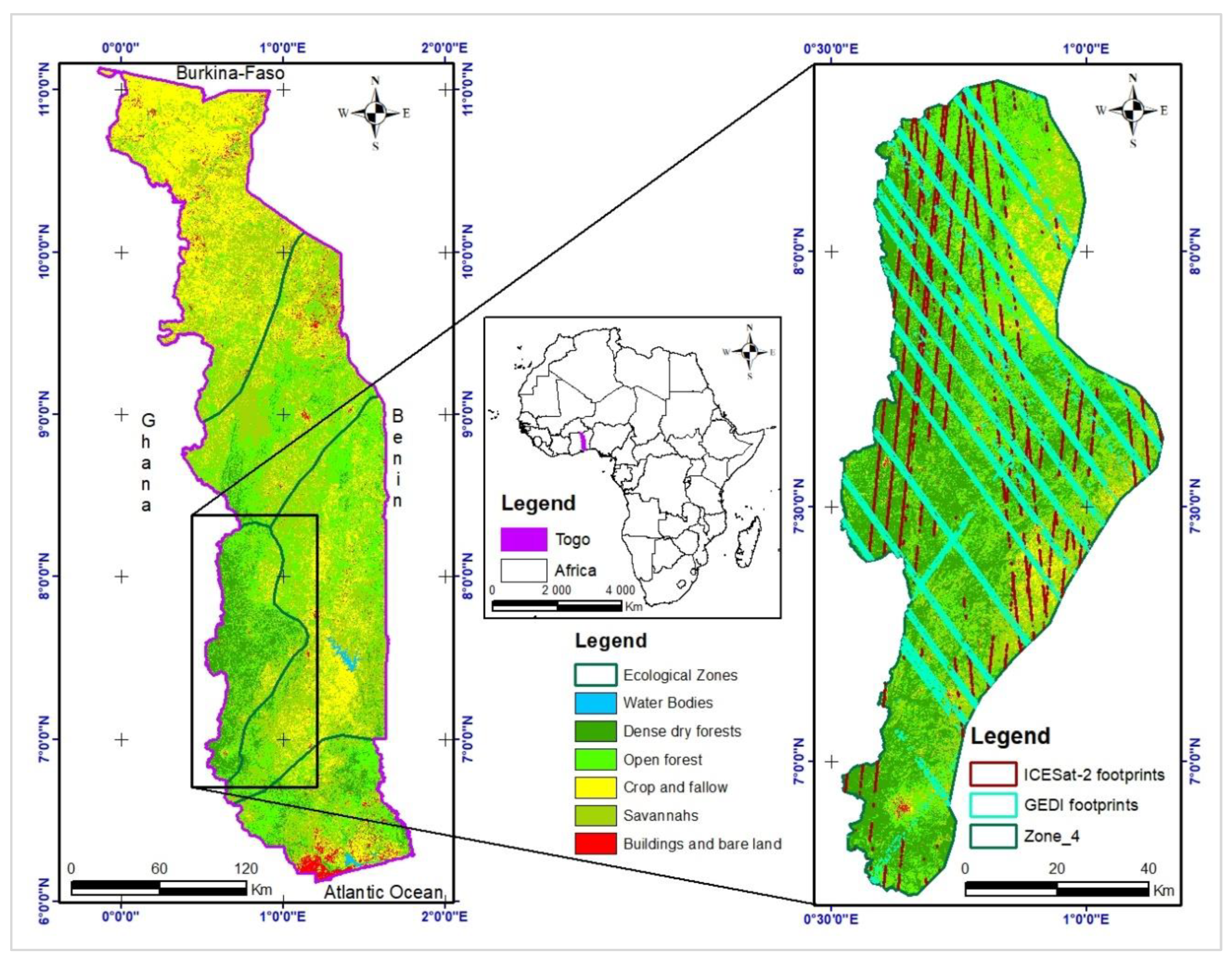
Figure 2.
Flowchart of the research methodology.
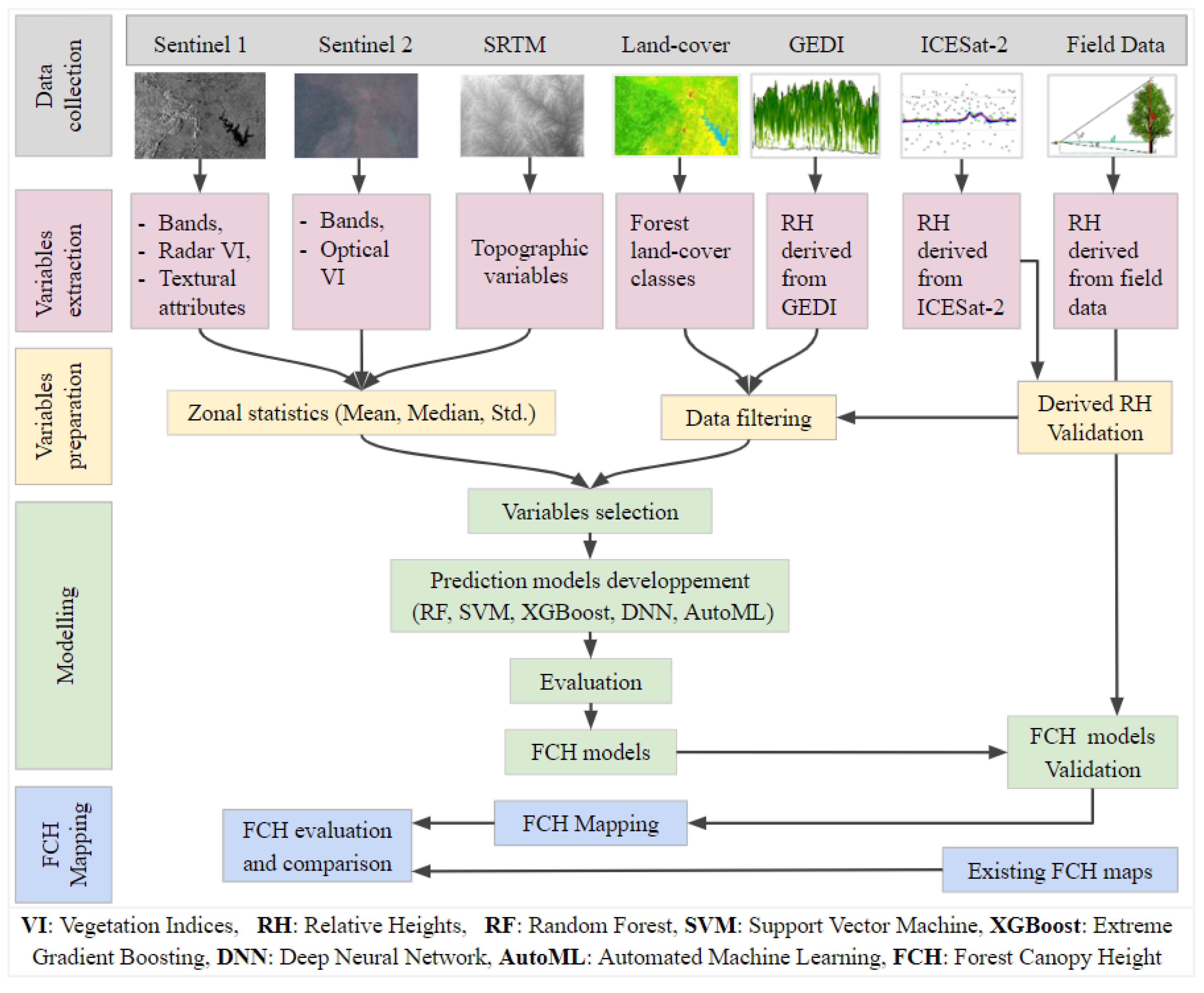
Figure 3.
Illustrative diagram of the structure of ICESat-2 (a) and GEDI (b) footprints.
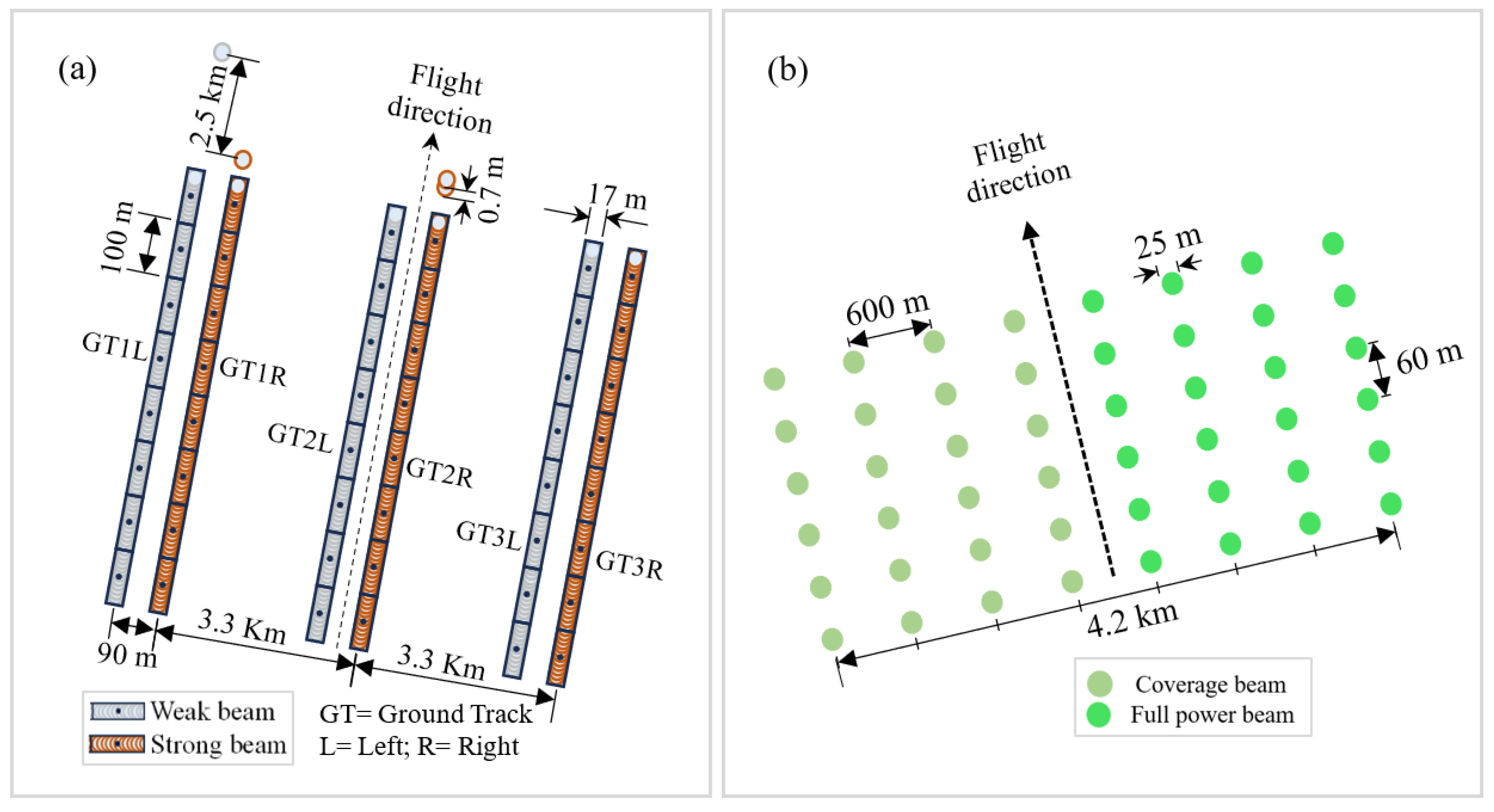
Figure 4.
Illustration of the overlay of GEDI and ICESat-2 data onto the VH band from Sentinel 1 to calculate zonal statistics.
Figure 4.
Illustration of the overlay of GEDI and ICESat-2 data onto the VH band from Sentinel 1 to calculate zonal statistics.
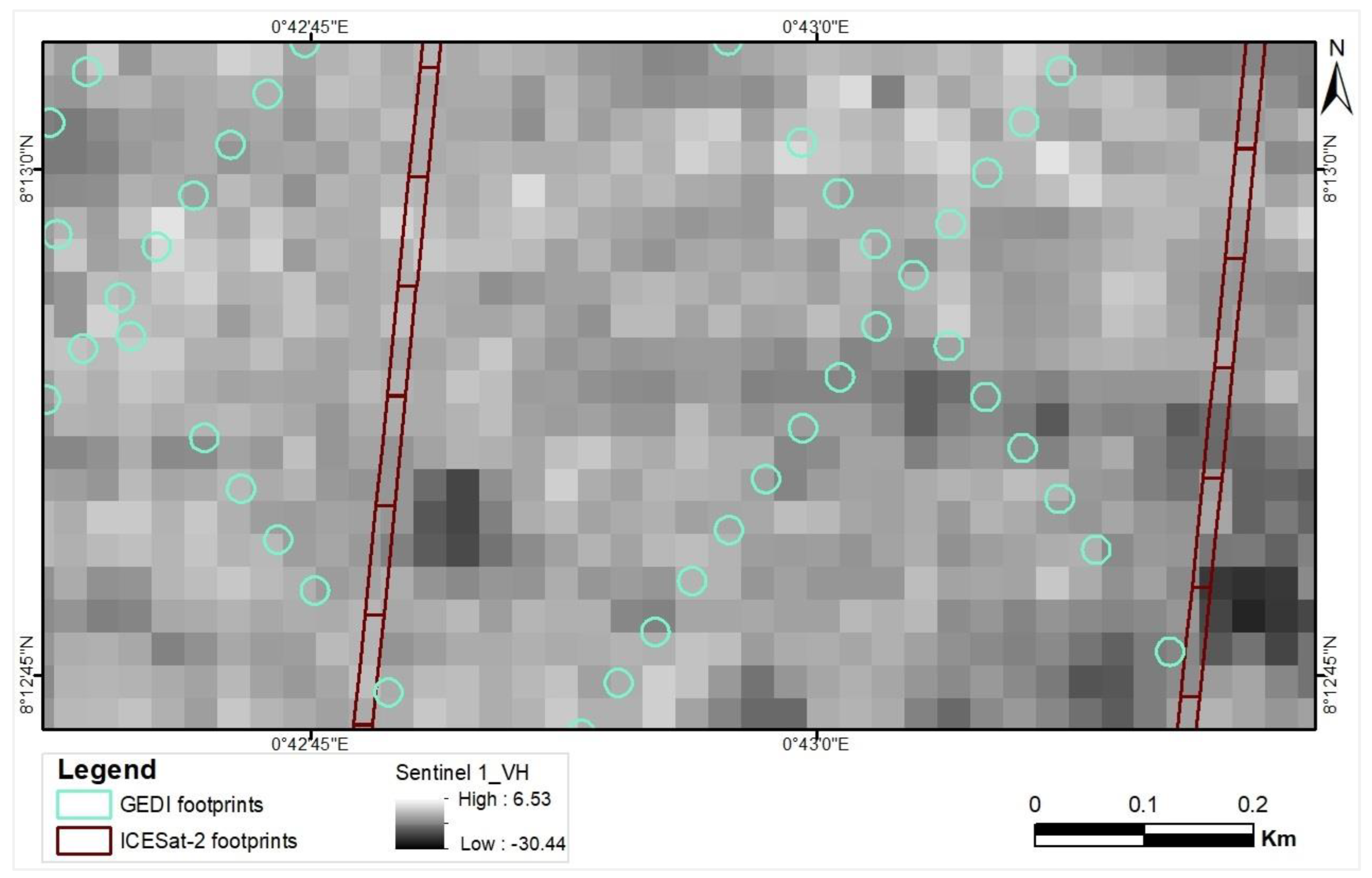
Figure 5.
Illustration of map inference from GEDI- or ICESat-2-based models.
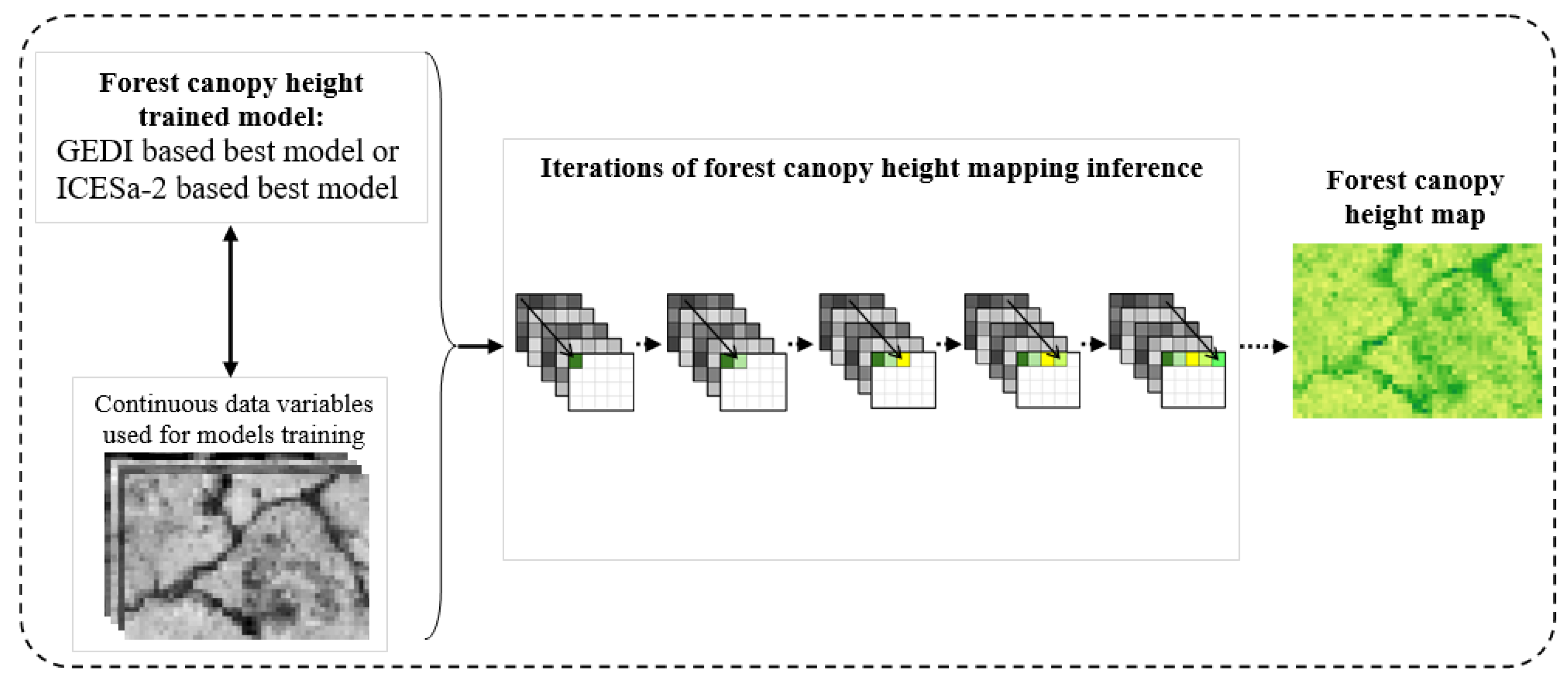
Figure 6.
Importance of variables with the RF module.
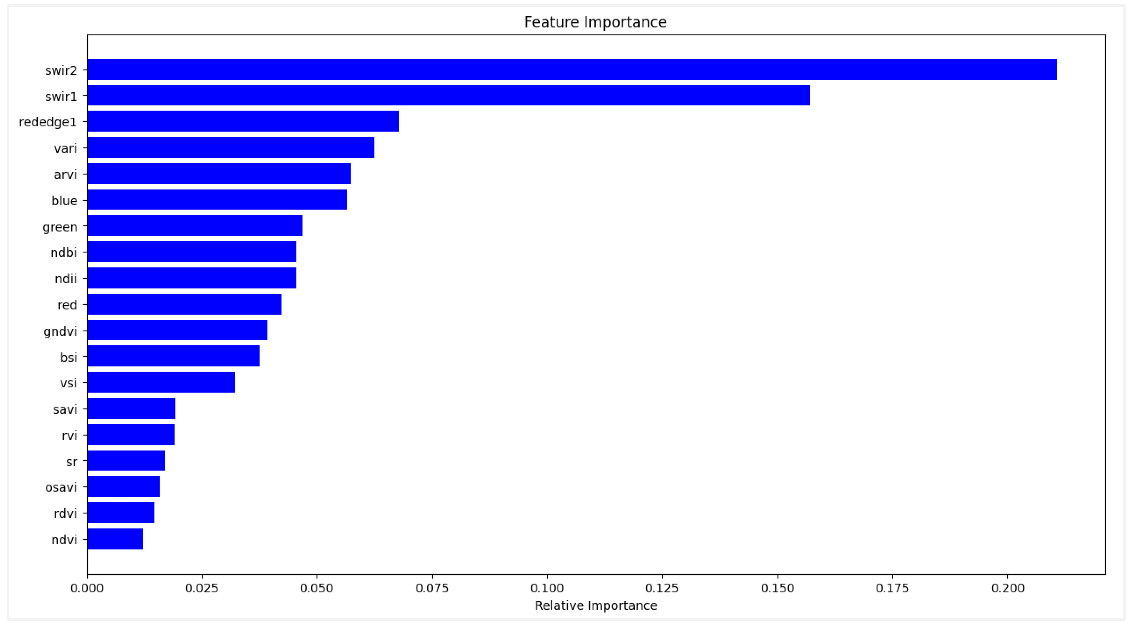
Figure 7.
Importance of features evaluated with SHAP with respect to height prediction with RF (a) and XGBoost (b) algorithms. Variable abbreviations are defined in Table 2 (Section 2.4).
Figure 7.
Importance of features evaluated with SHAP with respect to height prediction with RF (a) and XGBoost (b) algorithms. Variable abbreviations are defined in Table 2 (Section 2.4).
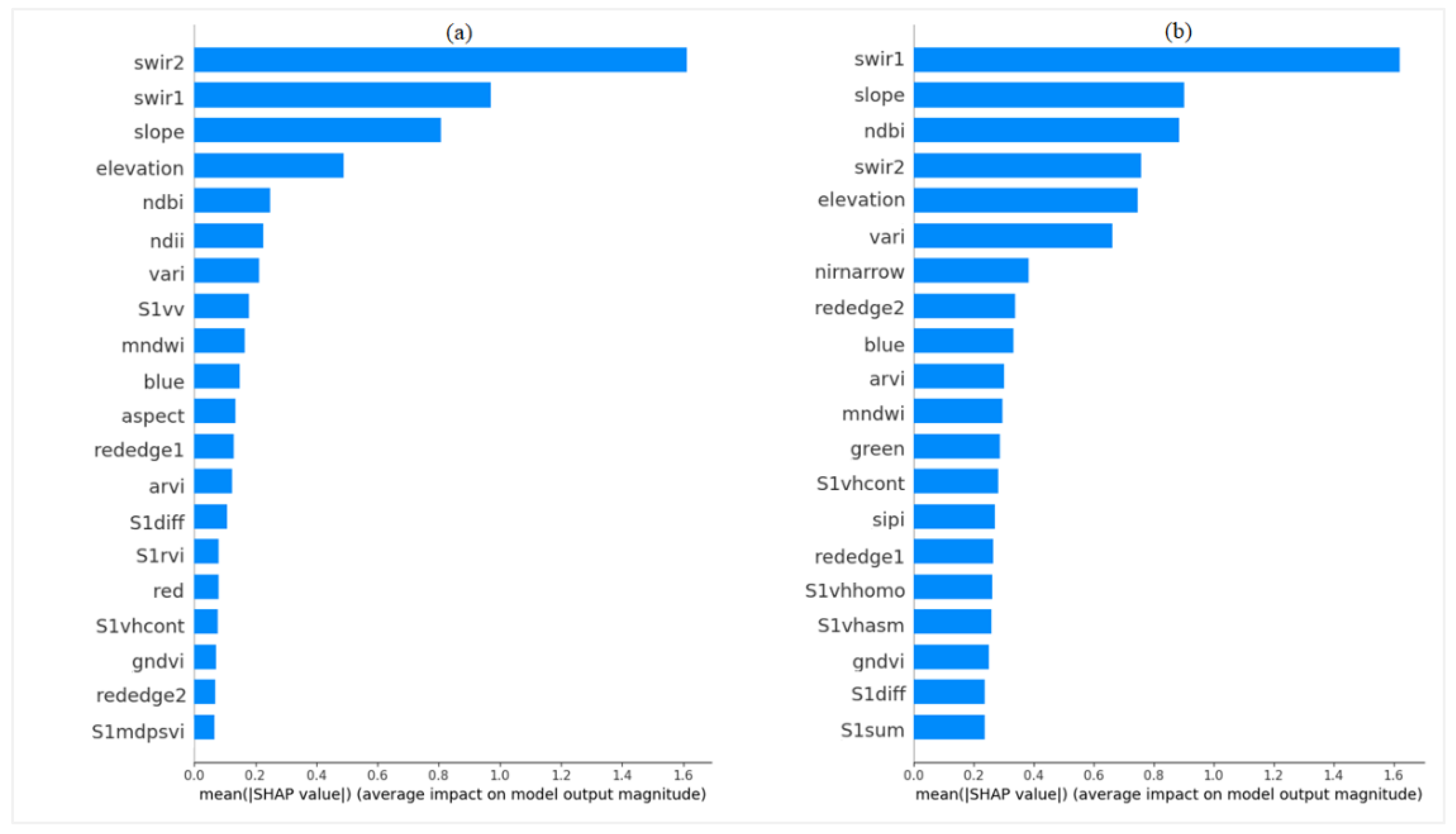
Figure 8.
Processing chain for the choice of the prediction model with ICESat-2 data.
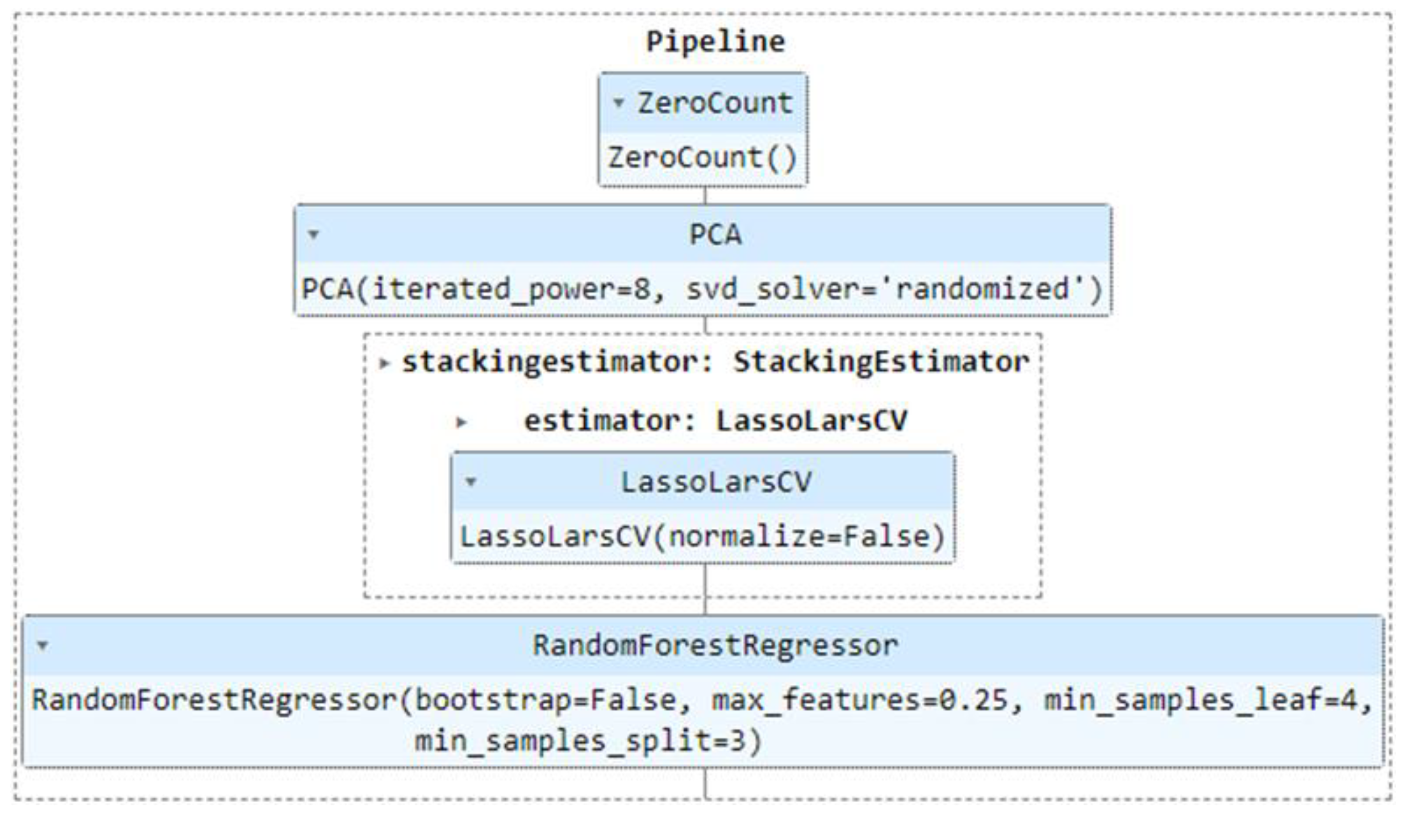
Figure 9.
Predicted vs observed values when modelling canopy height with ICESat-2 data.
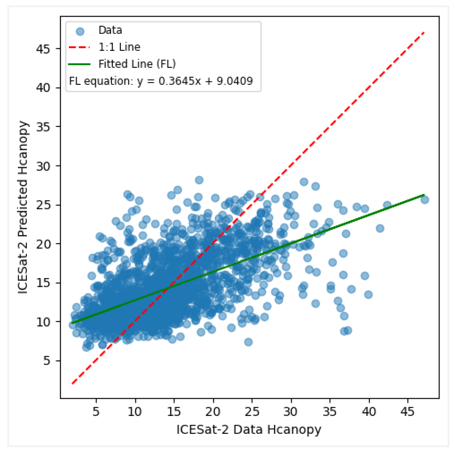
Figure 10.
Processing chain for the best prediction model with GEDI data.
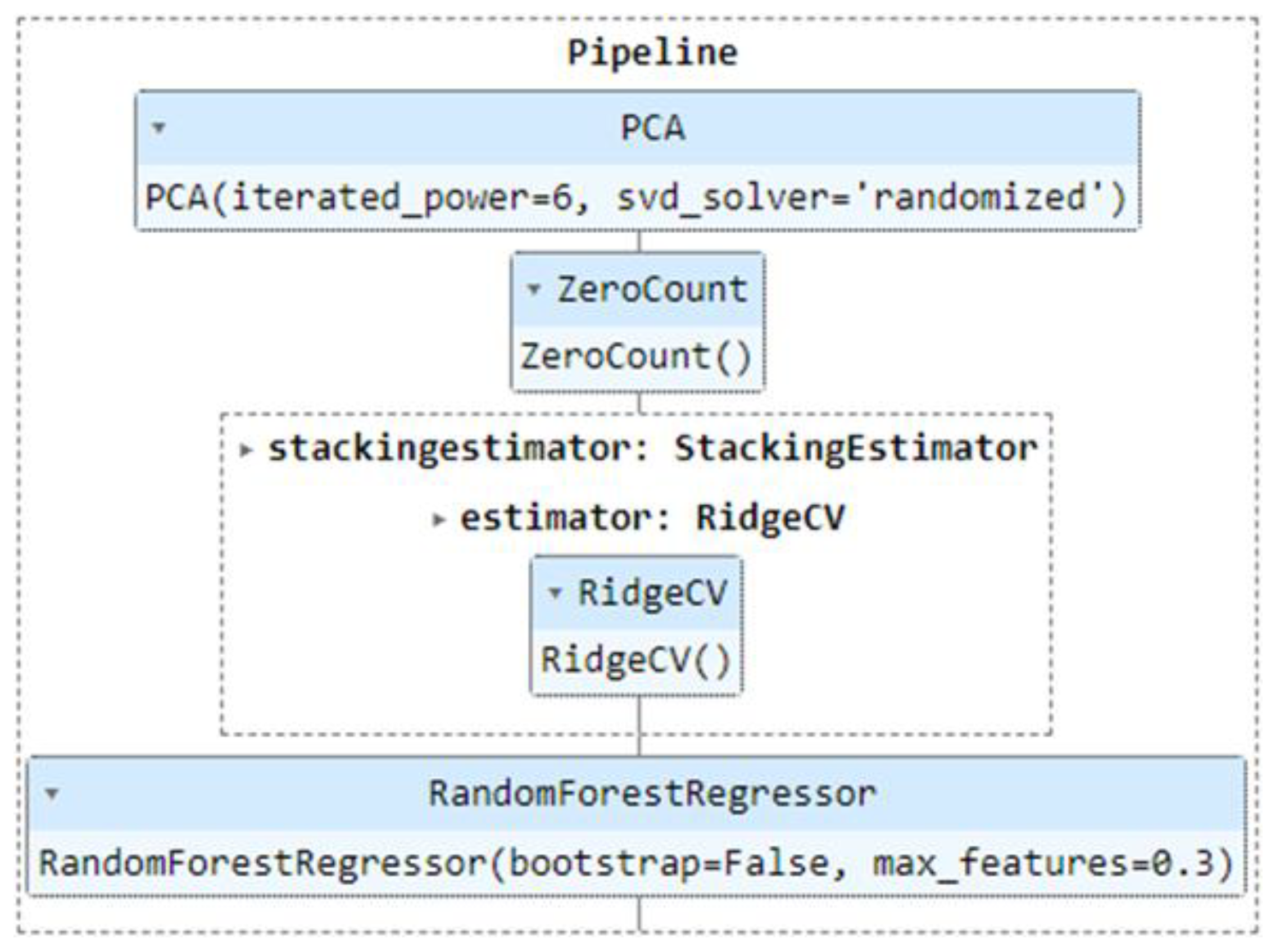
Figure 11.
Predicted vs observed values when modelling canopy height with GEDI data.
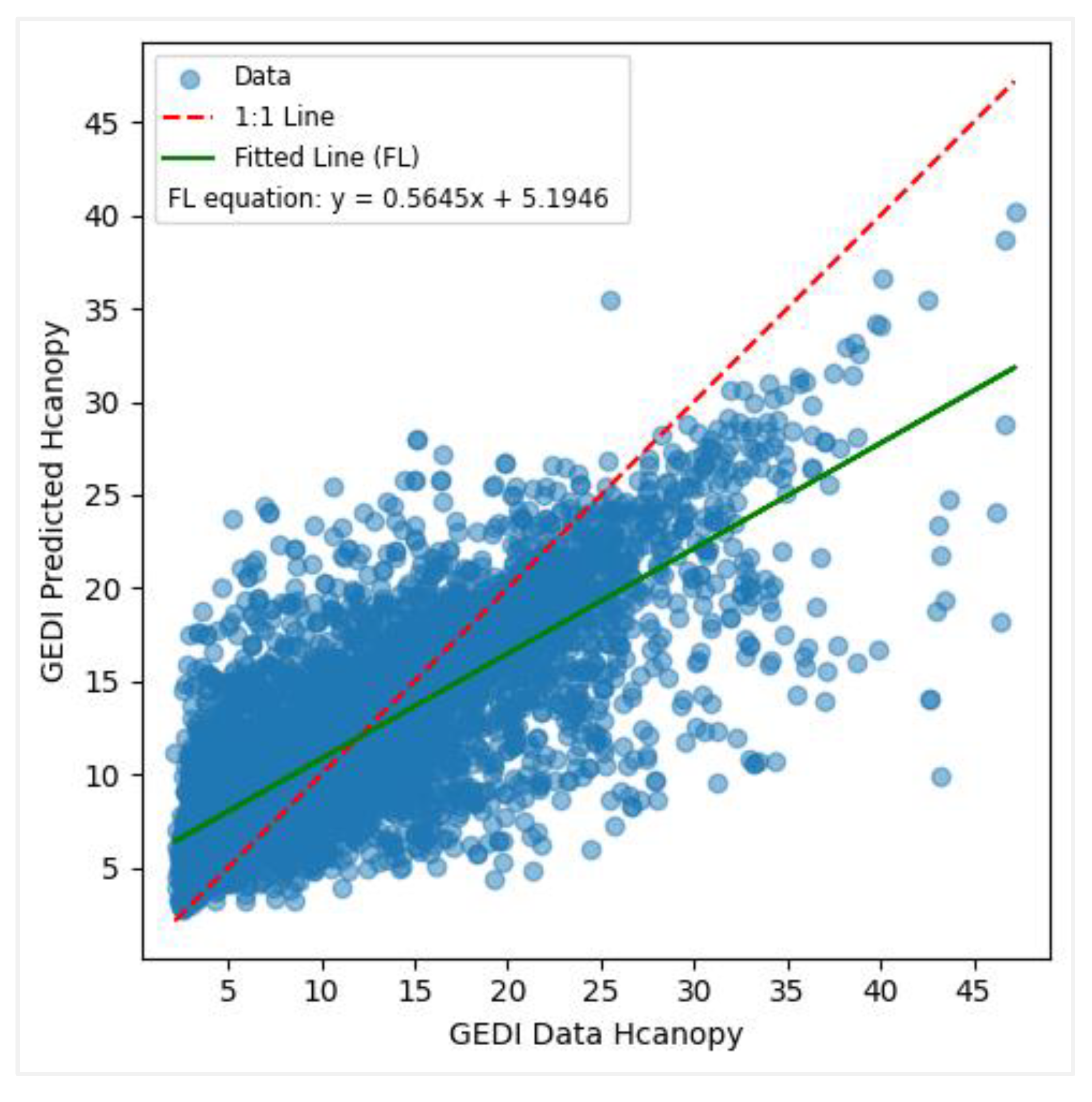
Figure 12.
Map of canopy heights estimated from ICESat-2 data.
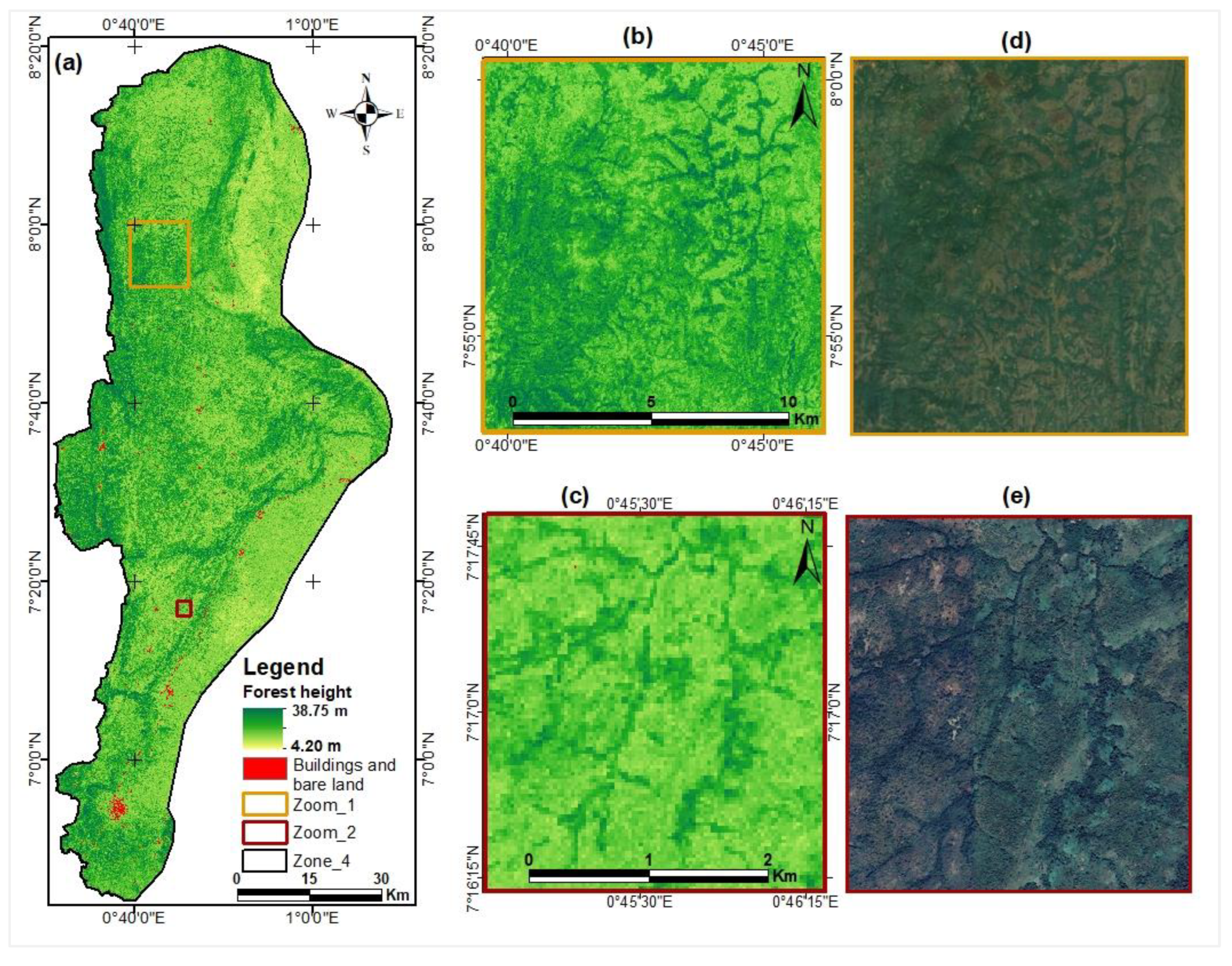
Figure 13.
Map of canopy heights estimated from GEDI data.
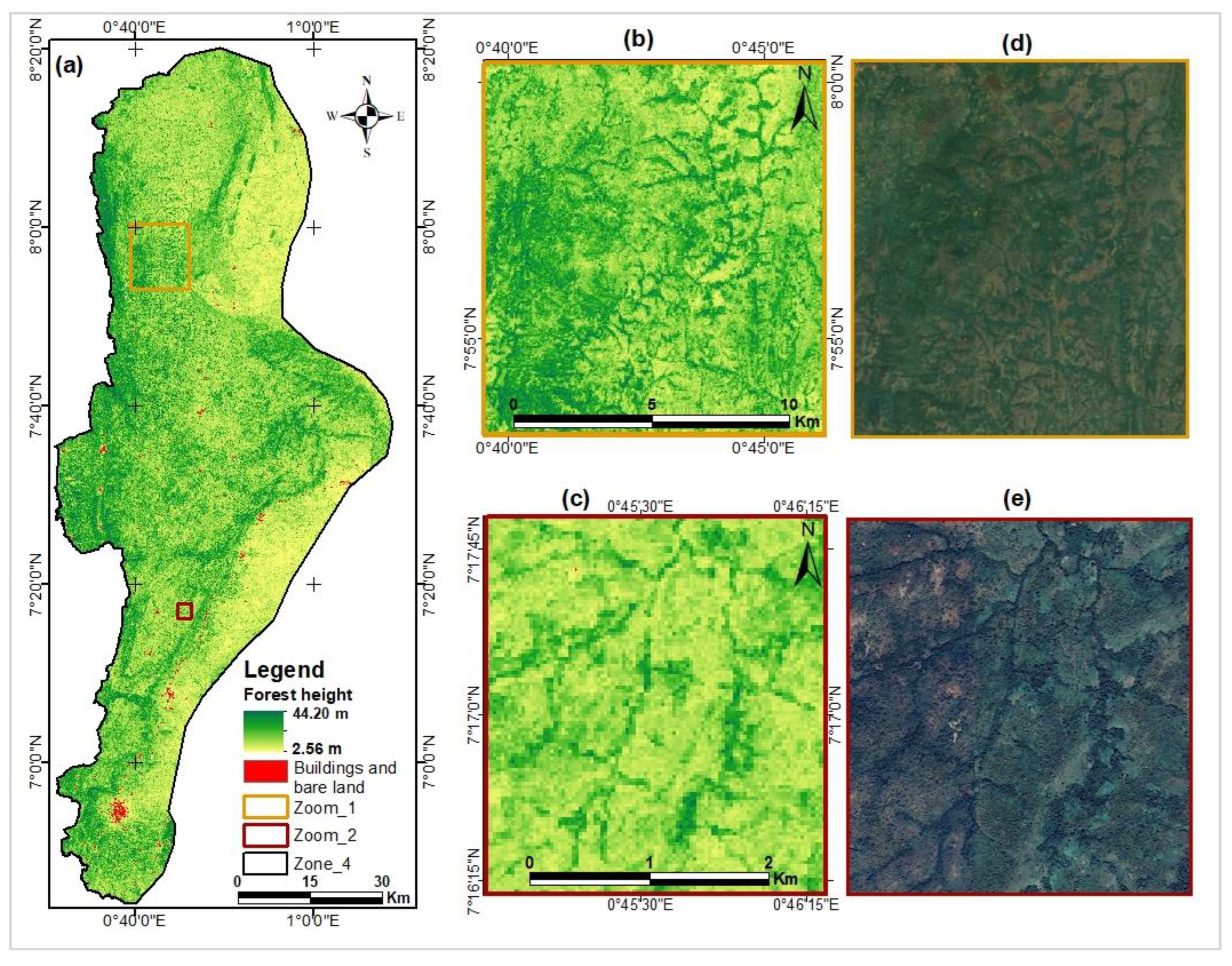
Figure 14.
Histograms of GEDI-based (a) and ICESat-2-based (b) maps, and the difference between GEDI/ICESat-2 maps (c).
Figure 14.
Histograms of GEDI-based (a) and ICESat-2-based (b) maps, and the difference between GEDI/ICESat-2 maps (c).
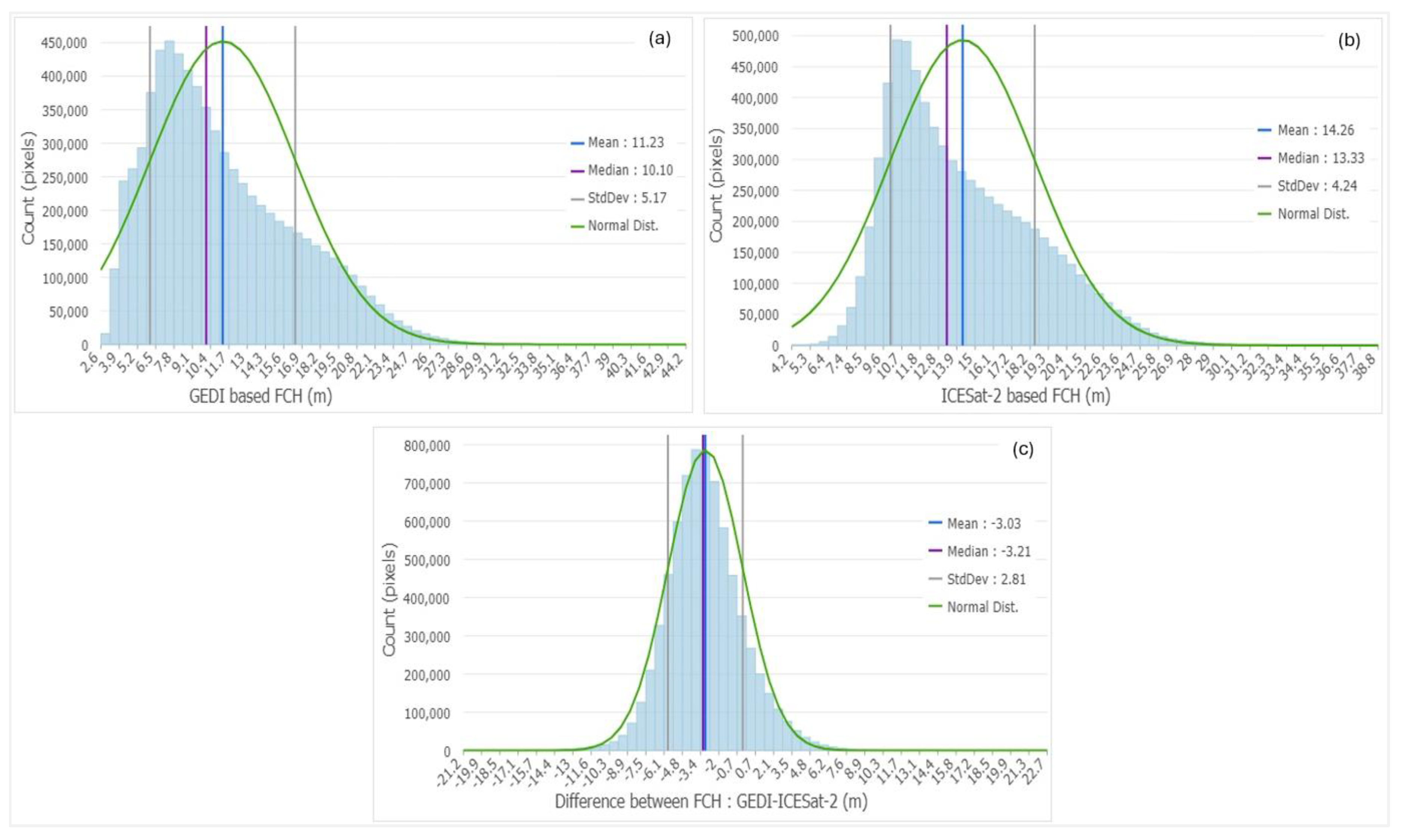
Figure 15.
Histograms of difference maps between GEDI/Lang (a) & GEDI/Potapov (b) maps.
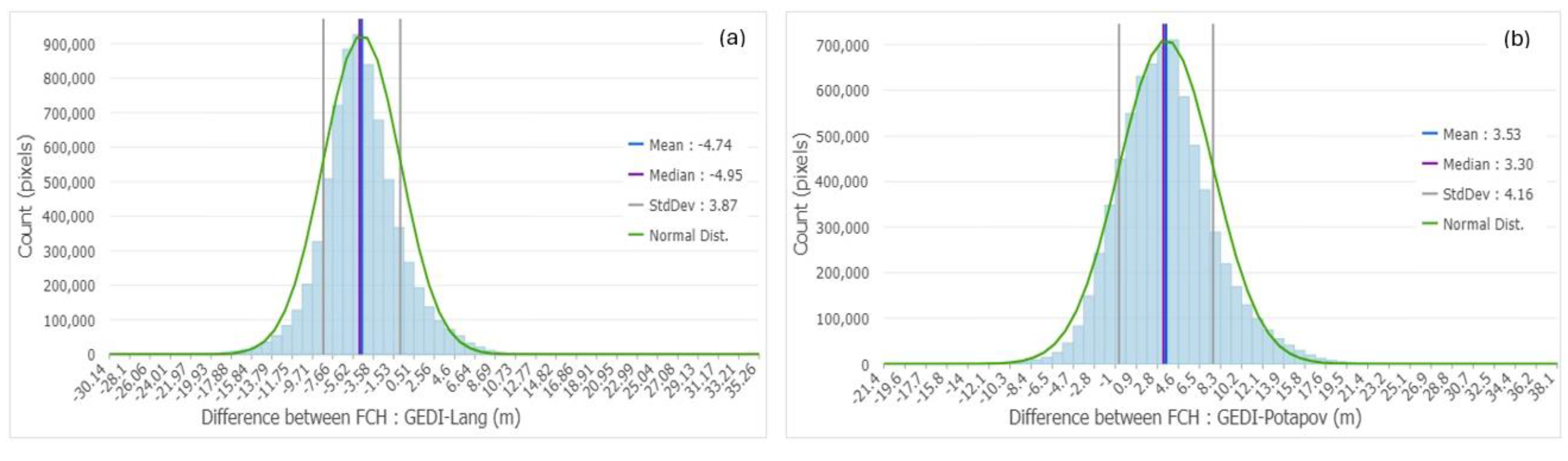
Table 1.
Data used in the research.
| Data source | Type of data | Year | Spatial resolution | Brief description |
|---|---|---|---|---|
| GEDI | Satellite LiDAR | 2020 | 25 m diameter | GEDI02_A granules containing relative canopy heights and other variables |
| ICESat-2 | Satellite LiDAR | 2020 | 17 m x 100 m | ATL08 products containing relative canopy heights and other variables |
| Sentinel 1 | Radar | 2020 | 10 m x 10 m | Synthetic Aperture Radar (SAR) images from the Sentinel-1A satellite |
| Sentinel 2 | Optical | 2020 | 10 m x 10 m,20 m x 20 m | Multi-spectral images from the Sentinel-2A satellite |
| SRTM | Altimetry | 2000 | 30 m x 30 m | Digital Terrain Model |
| Field plots &NFI2 plots | Dendrometry | 2020 2021 | 17 m x 100 m, &40 m diameter | Individual tree height & diameters at breast height (DBH) |
| Land use map | Cartography | 2020 | 30 m x 30 m | Existing land use map based on Landsat 8 data |
Table 2.
Covariates extracted from Sentinel 1, Sentinel 2, and SRTM data.
| Sentinel 1 | Description | Sentinel 2 | Description | SRTM | Description |
|---|---|---|---|---|---|
| S1vv | Sentinel1 Vertical transmit, Vertical receive polarisation | blue | Sentinel2 B2 | aspect | SRTM aspect |
| S1vh | Sentinel1 Vertical transmit, Horizontal receive polarisation | green | Sentinel2 B3 | elevation | SRTM elevation |
| S1diff | Sentinel1 Bands difference between VV and VH | red | Sentinel2 B4 | slope | SRTM slope |
| S1mdpsvi | Sentinel1 Modified Dual Polarimetric Sar Vegetation Index | rededge1 | Sentinel2 B5 | ||
| S1npdi | Sentinel1 Normalized Polarization Difference Index | rededge2 | Sentinel2 B6 | ||
| S1prod | Sentinel1 Bands product between VV and VH | rededge3 | Sentinel2 B7 | ||
| S1rept | Sentinel1 Bands report between VV and VH | nir | Sentinel2 B8 | ||
| S1rvi | Sentinel1 Ratio Vegetation Index | nirnarrow | Sentinel2 B8A | ||
| S1sum | Sentinel1 Bands sum between VV and VH | swir1 | Sentinel2 B11 | ||
| S1vhasm | Sentinel1 VH GLCM Angular Second Moment | swir2 | Sentinel2 B12 | ||
| S1vhcont | Sentinel1 VH GLCM Contrast | arvi | Atmospherically Resistant Vegetation Index | ||
| S1vhcorr | Sentinel1 VH GLCM Correlation | bsi | Bare Soil Index | ||
| S1vhdiss | Sentinel1 VH GLCM Dissimilarity | evi | Enhanced Vegetation Index | ||
| S1vhener | Sentinel1 VH GLCM Energy | gndvi | Green Normalized Difference Vegetation Index | ||
| S1vhent | Sentinel1 VH GLCM Entropy | mndwi | Modified Normalized Difference Water Index | ||
| S1vhhomo | Sentinel1 VH GLCM Inverse Difference Moment (Homogeneity) | msavi | Modified Soil Adjusted Vegetation Index | ||
| S1vhmax | Sentinel1 VH GLCM Maximum | mtvi | Modified Triangular Vegetation Index | ||
| S1vhmean | Sentinel1 VH GLCM Mean | ndbi | Normalized Difference Built-up Index | ||
| S1vhvar | Sentinel1 VH GLCM Variance | ndii | Normalized Difference Infrared Index | ||
| S1vvasm | Sentinel1 VV GLCM Angular Second Moment | ndvi | Normalized Difference Vegetation Index | ||
| S1vvcont | Sentinel1 VV GLCM Contrast | osavi | Optimized Soil Adjusted Vegetation Index | ||
| S1vvcorr | Sentinel1 VV GLCM Correlation | rdvi | Renormalized Difference Vegetation Index | ||
| S1vvdiss | Sentinel1 VV GLCM Dissimilarity | rvi | Ratio Vegetation Index | ||
| S1vvener | Sentinel1 VV GLCM Energy | savi | Soil Adjusted Vegetation Index | ||
| S1vvent | Sentinel1 VV GLCM Entropy | sipi | Structure Insensitive Pigment Index | ||
| S1vvhomo | Sentinel1 VV GLCM Inverse Difference Moment (Homogeneity) | sr | Simple Ratio | ||
| S1vvmax | Sentinel1 VV GLCM Maximum | vari | Visible Atmospherically Resistant Index | ||
| S1vvmean | Sentinel1 VV GLCM Mean | vsi | Vegetation Structure Index | ||
| S1vvvar | Sentinel1 VV GLCM Variance |
Table 3.
Selection configurations for GEDI data footprints for modelling.
| Configurations | Sensitivity | Quality_flag | Beam type | Acquisition time |
|---|---|---|---|---|
| Config1 | All beams | All beams | All beams | All beams |
| Config2 | ≥ 0 | 1 | Power | Day |
| Config3 | ≥ 0 | 1 | Power | Night |
| Config4 | ≥ 0 | 1 | Coverage | Day |
| Config5 | ≥ 0 | 1 | Coverage | Night |
| Config6 | ≥ 0.9 | 1 | Power | Day |
| Config7 | ≥ 0.9 | 1 | Power | Night |
| Config8 | ≥ 0.9 | 1 | Coverage | Day |
| Config9 | ≥ 0.9 | 1 | Coverage | Night |
Table 4.
Different scenarios for combining LiDAR variables with other multisource variables.
| Scenarios | Variable combinations | Number of variables |
|---|---|---|
| S1 | Optical | 28 |
| S2 | Radar | 29 |
| S3 | Topographic | 03 |
| S4 | Optical - Radar | 57 |
| S5 | Optical - Topographical | 31 |
| S6 | Radar - Topographical | 32 |
| S7 | Optical - Radar - Topographical | 60 |
Table 5.
ICESat-2 Data Validation Correlation Matrix.
| Min. | 1st Qu. | Med | Mean | Max. | RH50 | RH55 | RH60 | RH65 | RH70 | RH75 | RH80 | RH85 | RH90 | RH95 | RH98 | h_canopy | |
|---|---|---|---|---|---|---|---|---|---|---|---|---|---|---|---|---|---|
| Min. | 1 | ||||||||||||||||
| 1st Qu. | 0.76 | 1 | |||||||||||||||
| Med | 0.65 | 0.92 | 1 | ||||||||||||||
| Mean | 0.64 | 0.88 | 0.95 | 1 | |||||||||||||
| Max. | 0.23 | 0.4 | 0.48 | 0.67 | 1 | ||||||||||||
| RH50 | 0.65 | 0.92 | 1 | 0.95 | 0.48 | 1 | |||||||||||
| RH55 | 0.61 | 0.89 | 0.99 | 0.96 | 0.5 | 0.99 | 1 | ||||||||||
| RH60 | 0.58 | 0.87 | 0.98 | 0.96 | 0.52 | 0.98 | 0.99 | 1 | |||||||||
| RH65 | 0.56 | 0.83 | 0.95 | 0.96 | 0.54 | 0.95 | 0.97 | 0.99 | 1 | ||||||||
| RH70 | 0.53 | 0.8 | 0.93 | 0.96 | 0.56 | 0.93 | 0.95 | 0.97 | 0.99 | 1 | |||||||
| RH75 | 0.5 | 0.77 | 0.91 | 0.95 | 0.58 | 0.91 | 0.93 | 0.95 | 0.98 | 0.99 | 1 | ||||||
| RH80 | 0.47 | 0.73 | 0.87 | 0.94 | 0.63 | 0.87 | 0.9 | 0.92 | 0.95 | 0.97 | 0.98 | 1 | |||||
| RH85 | 0.45 | 0.69 | 0.83 | 0.94 | 0.68 | 0.83 | 0.86 | 0.89 | 0.92 | 0.93 | 0.95 | 0.98 | 1 | ||||
| RH90 | 0.42 | 0.65 | 0.78 | 0.91 | 0.75 | 0.78 | 0.81 | 0.83 | 0.86 | 0.88 | 0.9 | 0.94 | 0.97 | 1 | |||
| RH95 | 0.37 | 0.56 | 0.68 | 0.85 | 0.83 | 0.68 | 0.71 | 0.73 | 0.75 | 0.78 | 0.8 | 0.84 | 0.88 | 0.94 | 1 | ||
| RH98 | 0.31 | 0.49 | 0.59 | 0.78 | 0.92 | 0.59 | 0.62 | 0.64 | 0.66 | 0.69 | 0.71 | 0.76 | 0.81 | 0.87 | 0.96 | 1 | |
| h_canopy | 0.11 | 0.23 | 0.32 | 0.41 | 0.49 | 0.32 | 0.33 | 0.34 | 0.36 | 0.39 | 0.41 | 0.42 | 0.45 | 0.5 | 0.52 | 0.53 | 1 |
Table 6.
Accuracy metrics of the prediction models for the seven scenarios.
| Models | RF | SVM | XGBoost | DNN | ||||||
|---|---|---|---|---|---|---|---|---|---|---|
| Scenarios | S1 | S2 | S3 | S4 | S5 | S6 | S7 | S7 | S7 | S7 |
| r | 0.53 | 0.26 | 0.28 | 0.56 | 0.57 | 0.46 | 0.62 | 0.53 | 0.57 | 0.57 |
| RMSE | 5.72 | 6.25 | 6.57 | 5.52 | 5.40 | 9.96 | 5.28 | 5.50 | 5.21 | 5.68 |
| MAE | 4.23 | 4.70 | 4.88 | 4.15 | 3.92 | 4.44 | 4.00 | 4.08 | 4.06 | 4.11 |
Table 7.
Canopy height prediction models from GEDI data.
| Relative Height | Config1 | Config2 | Config3 | Config4 | Config5 | Config6 | Config7 | Config8 | Config9 |
|---|---|---|---|---|---|---|---|---|---|
| Pearson Correlation Coefficient (r) | |||||||||
| RH75 | 0.55 | 0.60 | 0.67 | 0.59 | 0.76 | 0.59 | 0.69 | 0.67 | 0.77 |
| RH80 | 0.57 | 0.54 | 0.69 | 0.67 | 0.78 | 0.56 | 0.69 | 0.67 | 0.78 |
| RH85 | 0.56 | 0.61 | 0.69 | 0.66 | 0.76 | 0.58 | 0.69 | 0.65 | 0.77 |
| RH90 | 0.56 | 0.61 | 0.71 | 0.62 | 0.77 | 0.54 | 0.70 | 0.63 | 0.77 |
| RH95 | 0.58 | 0.58 | 0.70 | 0.61 | 0.77 | 0.58 | 0.70 | 0.64 | 0.77 |
| RH98 | 0.58 | 0.61 | 0.70 | 0.67 | 0.77 | 0.58 | 0.71 | 0.68 | 0.80 |
| RH100 | 0.59 | 0.59 | 0.69 | 0.69 | 0.73 | 0.59 | 0.69 | 0.65 | 0.77 |
| Root Mean Squared Error (RMSE) | |||||||||
| RH75 | 6.04 | 5.06 | 4.83 | 4.21 | 3.91 | 5.22 | 5.00 | 3.68 | 3.84 |
| RH80 | 6.17 | 5.75 | 5.03 | 3.91 | 4.01 | 5.66 | 5.09 | 3.83 | 4.01 |
| RH85 | 6.61 | 5.62 | 5.32 | 4.25 | 4.39 | 5.87 | 5.27 | 4.33 | 4.28 |
| RH90 | 6.90 | 5.97 | 5.57 | 4.48 | 4.51 | 5.90 | 5.45 | 4.48 | 4.53 |
| RH95 | 6.88 | 6.33 | 5.91 | 4.73 | 4.62 | 6.50 | 5.85 | 4.89 | 4.69 |
| RH98 | 7.19 | 6.70 | 6.10 | 4.56 | 4.71 | 6.83 | 6.09 | 4.48 | 4.42 |
| RH100 | 7.23 | 6.59 | 6.18 | 4.45 | 5.09 | 6.67 | 6.17 | 4.75 | 4.90 |
| Mean Absolute Error (MAE) | |||||||||
| RH75 | 3.91 | 3.70 | 3.30 | 3.04 | 2.72 | 3.80 | 3.40 | 2.61 | 2.65 |
| RH80 | 4.07 | 4.20 | 3.51 | 2.80 | 2.84 | 4.20 | 3.53 | 2.89 | 2.83 |
| RH85 | 4.41 | 4.26 | 3.75 | 3.13 | 3.11 | 4.37 | 3.74 | 3.12 | 3.07 |
| RH90 | 4.63 | 4.51 | 4.03 | 3.35 | 3.30 | 4.48 | 3.95 | 3.31 | 3.24 |
| RH95 | 4.77 | 4.89 | 4.35 | 3.54 | 3.36 | 4.87 | 4.29 | 3.53 | 3.42 |
| RH98 | 4.95 | 5.03 | 4.55 | 3.36 | 3.43 | 5.24 | 4.51 | 3.40 | 3.15 |
| RH100 | 5.03 | 5.12 | 4.64 | 3.34 | 3.83 | 5.16 | 4.61 | 3.53 | 3.52 |
Note: Rank ordering of nine configurations based on three Random Forest performance metrics. Pearson r: 6 = 1 < 2 < 4 = 8 < 3 = 7 < 5 = 9. W = 0.951, c2r = 53.26, df = 8, p < 0.0001. RMSE: 1 < 6 = 2 < 3 = 7 < 5 = 4 ≤ 9 = 8. W = 0.847, c2r = 47.41, df = 8, p < 0.0001. MAE: 6 ≤ 2 = 1 < 3 = 7 < 4 = 5 < 8 < 9. W = 0.912, c2r = 51.08, df = 8, p < 0.0001.
Table 8.
Effects of Auto-ML TPOT and AutoGluon on model performance.
| Data | Models | r | RMSE | MAE |
|---|---|---|---|---|
| ICESat-2 | RF | 0.61 | 5.40 | 3.81 |
| AutoGluon (RF) | 0.64 | 5.12 | 3.83 | |
| TPOT (RF) | 0.65 | 5.10 | 3.80 | |
| GEDI | RF | 0.80 | 4.42 | 3.15 |
| AutoGluon (RF) | 0.83 | 4.16 | 2.65 | |
| TPOT (RF) | 0.84 | 4.15 | 2.36 |
Table 9.
Correlations between extracted or existing data versus predicted data.
| No. | Regression data | r | RMSE | MAE |
|---|---|---|---|---|
| 1 | ICESat-2_Data / Field_data | 0.53 | 4.85 | 3.84 |
| 2 | ICESat-2_Model / Field_data | 0.54 | 3.11 | 2.54 |
| 3 | ICESat-2_Data / Lang | 0.60 | 3.66 | 2.80 |
| 4 | ICESat-2_Model / Lang | 0.71 | 3.38 | 2.55 |
| 5 | ICESat-2_Data / Potapov | 0.52 | 3.15 | 2.39 |
| 6 | ICESat-2_Model / Potapov | 0.62 | 3.80 | 2.93 |
| 7 | ICESat-2_ Model / NFI2 | 0.55 | 3.65 | 2.98 |
| 8 | GEDI_Data / Lang | 0.64 | 3.90 | 2.94 |
| 9 | GEDI_Model / Lang | 0.65 | 5.50 | 4.17 |
| 10 | GEDI_Data / Potapov | 0.54 | 4.11 | 3.15 |
| 11 | GEDI_ Model / Potapov | 0.55 | 6.04 | 4.64 |
| 12 | GEDI_ Model / NFI2 | 0.63 | 3.40 | 2.65 |
| 13 | Lang / INFI2 | 0.64 | 3.96 | 3.09 |
| 14 | Potapov / NFI2 | 0.46 | 4.21 | 3.28 |
Note: Models are set in boldface for the highest correlations using the ICESat-2 and GEDI datasets versus field measurements, NFI2, and Lang and Potapov datasets.
Disclaimer/Publisher’s Note: The statements, opinions and data contained in all publications are solely those of the individual author(s) and contributor(s) and not of MDPI and/or the editor(s). MDPI and/or the editor(s) disclaim responsibility for any injury to people or property resulting from any ideas, methods, instructions or products referred to in the content. |
© 2024 by the authors. Licensee MDPI, Basel, Switzerland. This article is an open access article distributed under the terms and conditions of the Creative Commons Attribution (CC BY) license (http://creativecommons.org/licenses/by/4.0/).
Copyright: This open access article is published under a Creative Commons CC BY 4.0 license, which permit the free download, distribution, and reuse, provided that the author and preprint are cited in any reuse.


