
Submitted:
16 December 2024
Posted:
17 December 2024
You are already at the latest version
Abstract
Forest attributes such as the standing stock, diameter at the breast height, tree height, and basal area, are essential in forest management. Conventional estimation methods, which are still largely used in many parts of the world, are typically resource intensive. Machine learning algorithms working with remotely sensed data trained by ground measurements may provide a promising, more efficient alternative. This study evaluates the performance of three machine learning algo-rithms, namely Random Forest, Classification and Regression Trees, and Gradient Boosting Tree Algorithm in estimating these forest attributes. Ground truth data was sourced by measurements carried out in relevant forests from Romania and by an independent dataset from Brasov County. The predictive ability of the tested algorithms was examined by considering several spatial resolu-tions. The results showed varying degrees of performance. Random Forest was the best performer, with RMSE and R2 values over 0.8 for all attributes. GBTA excelled in predicting the standing stock, achieving R2 values over 0.9. The validation based on the independent dataset has confirmed higher performance for both RF and GBTA. In contrast, CART excelled in predicting the basal area, but struggled with breast height diameter, standing stock, and tree height. A sensitivity analysis that concerned the spatial resolution revealed high degrees of discrepancy. Random Forest and Gradient Boosting Tree Algorithm were more consistent when estimating the standing stock, but they have shown inconsistency for breast height diameter and tree height, while CART showed important variations. These results provide useful insights into the strengths and weaknesses of these algo-rithms, and provide the information required to select the best option when aiming to use similar solutions for estimation.
Keywords:
spatial resolution
; machine learning
; remotely sensed data
; prediction
; forest attributes
; performance
; decision
1. Introduction
Forests are vital ecosystems, offering a diverse array of provisioning, regulating, cultural, and supporting services [1,2,3], thus playing a critical role in sustaining human well-being. Accurate and updated information on measurable forest attributes is essential for an effective forest management [4,5]. Typically, attributes such as the standing stock (Vol), basal area (BA), and aboveground biomass (AGB), are used to understand and differentiate forest structure and productivity [6,7]. For instance, estimates of standing stocks are essential for assessing timber quantity, in guiding sustainable harvesting practices, and ensuring the long-term viability of forest resources. Additionally, BA offers insights into stand density and overall forest health [6]. By understanding the spatial distribution and density of trees within a forest stand, managers can better plan, mitigate risks of disease and fire, and maintain ecosystem resilience [8]. In turn, AGB estimates are important in understanding the forests’ potential to store carbon, which is important to shape policies for decarbonization and to mitigate climate changes.
Typically, all these parameters are estimated based on manual ground measurements, standing for the conventional approach to the problem, which often involves resource-intensive field surveys, expertise, and working in adverse conditions [9] . Furthermore, conventional methods may not be scalable or cost-effective for large-scale biomass mapping and estimation efforts, particularly in remote or densely forested areas [10,11,12]. According to the methodology outlined by the Intergovernmental Panel on Climate Change (IPCC), as well as by several local guidelines and textbooks, the AGB of trees can be estimated using allometric equations parameterized with diameter at the breast height (DBH) and tree height (H) as primary variables [13]. These equations are designed to provide accurate biomass estimates by leveraging the correlation between tree size and biomass stored in it [13,14].
Despite the straightforward and reliable nature of DBH and H measurements across various forest types and regions, these persist as resource intensive and often lack scalability [15,16]. Integrating remote sensing technologies such as satellite imagery and LiDAR (Light Detection and Ranging) are promising in removing these limitations, making forest attribute estimation more efficient and cost-effective [17]. While these methods allow for broader coverage and can capture data in otherwise inaccessible regions, they require accurate ground truth data for validation and hold a limited ability to characterize the understory vegetation [17].
Regression algorithms have long been used as powerful tools for extrapolating field data and generating detailed maps of forest attributes [18,19]. These algorithms use statistical techniques to model the relationships between various forest attributes and environmental variables [20]. Integrating them with remotely sensed data offers a promising approach to improving forest management practices [11,21]. Forest managers, for instance, can gain valuable insights into various aspects of forest dynamics, including vegetation health and biodiversity distribution [22]. This combination enables a more accurate and efficient monitoring and assessment of forests at different scales, supporting decision-making in forest conservation, sustainable resource management, and the prevention of environmental threats [23,24].
Although various machine learning algorithms have been used in estimating forest attributes, the choice between parametric and non-parametric algorithms remains challenging [25,26]. Parametric algorithms, such as linear regression, rely on several assumptions about the data distribution and hold fixed parameters [27]. On the other hand, non-parametric algorithms, including Random Forest (RM) and Support Vector Machines (SVM), are more flexible because they can capture complex relationships without strict statistical assumptions [28]. Understanding the strengths and weaknesses of algorithms from this class is essential in selecting the optimal one for specific forest attribute estimation tasks.
Among non-parametric algorithms, RF, GBTA (Gradient Boosting Tree Algorithm) and CART (Classification and Regression Trees) have demonstrated their effectiveness in accurately estimating various forest characteristics such as the above ground biomass [29,30,31], forest canopy height [32] and standing stock [33,34]. The RF algorithm minimizes prediction variance in supervised machine learning by combining multiple decision trees through a process called bagging [35]. Initially, each tree is trained on random subsets of data; during validation, the algorithm averages the predictions to come at a balanced prediction outcome [35,36]. Its effectiveness lies in handling intricate decision boundaries for both categorical and continuous variables, managing noisy and high-dimensional datasets, and minimizing overfitting [37]. The algorithm incorporates randomization techniques to reduce tree correlation, which enhances the model accuracy. It excels in handling large datasets with numerous variables and complex interactions between them [23]. CART algorithm is a versatile binary recursive partitioning method for classification and regression tasks [38]. It constructs a tree structure by iteratively dividing data into increasingly homogeneous subsets based on selected features and threshold values; the process continues until stopping conditions, such as reaching maximum depth or a minimum number of samples per leaf node are met [28]. The resulting tree structure can be pruned to prevent overfitting, which improves the generalization capabilities [39]. CART accommodates both categorical and continuous variables, handles multi-class tasks, and provides interpretable decision trees for insights into feature-target connections [40]. GBTA is a powerful machine learning algorithm that enhances prediction accuracy by building an ensemble of decision trees based on the boosting concept [41]. As abovementioned methods, it corrects errors from previous models by iteratively fitting decision trees to residuals and preventing overfitting through regularization [28]. Popular implementations like XGBoost, LightGBM, and GBM, extend GBTA's capabilities, using different optimization techniques [42]. GBTA handles both numerical and categorical variables, demonstrating interpretability and robustness to noisy data; despite its versatility, achieving an optimal performance requires a meticulous hyperparameter tuning [39].
While some studies [30,43,44,45,46] have focused on specific forest attributes or localized areas, a significant gap remains in detailed national-scale mapping of forest attributes. Machine learning (ML) models perform best when training, validation, and testing occur within a well-defined domain. Localized data may introduce uncertainties in species diversity, topography, and forest density, which limit model generalizability. Moreover, ML models face challenges with intra- and inter-class similarity in spectral data, potentially leading to biased predictions. Addressing this requires diverse training datasets encompassing various forest types and topographies. Additionally, hyperparameter tuning may yield good results for a limited domain, but consistency is not guaranteed across broader or changing conditions. Thus, testing ML algorithms at national scales offers insights into their adaptability to varied landscapes [47]. Romania's diverse ecosystems provide an ideal setting for testing the generalizability of ML models [48]. Leveraging this biodiversity can help produce findings that are applicable to other temperate forests worldwide, contributing to improved forest management on both national and global scales [30,49].
The complexity of the model, including the number of parameters and features considered, plays an important role in determining its predictive capabilities [20]. Complex models may be able to capture intricate patterns and relationships within the data but may also be more prone to overfitting, especially when applied to larger spatial extents [50]. On the other hand, simpler models may generalize better but might struggle to capture fine-scale variations in forest attributes [20,43].
Additionally, the choice of spatial resolution affects the performance of machine learning algorithms at larger scales [51]. Coarser spatial resolutions may lead to loss of detail and less variability in the data, potentially affecting the accuracy of predictions [52]; conversely, finer spatial resolutions can provide more detailed information but may also increase computational complexity and resource requirements [49].
Some studies [53,54] advanced our understanding in mapping of forest attributes at a larger scale, such as the national level, but there remains a critical oversight regarding the process of testing on unseen data, which can be provided by independent datasets. This process is essential for assessing the generalizability and robustness of the models [26].
The aim of this study was to model forest characteristics in temperate forests, with a particular focus on Romania, using machine learning algorithms and remotely sensed data. By leveraging the power of machine learning and remote sensing technologies, we aimed to generate comprehensive and detailed maps of forest attributes. Romanian forests were considered representative of temperate forests globally, allowing for the extrapolation of findings to similar forest ecosystems worldwide. The following objectives were setup for this study: i) to compare the performance of three machine learning algorithms—Random Forest (RF), Gradient Boosting Tree Algorithm (GBTA), and Classification and Regression Trees (CART)—in predicting key forest attributes (e.g., standing stock volume, basal area, tree height) based on Sentinel-2 satellite data. This objective supports the selection of the appropriate algorithm by directly comparing different ML approaches, highlighting strengths and weaknesses in their predictions, ii) to evaluate the impact of model complexity on predictive accuracy, elucidating whether increased complexity leads to better performance. This objective aims to determine whether model complexity plays a significant role in improving prediction accuracy, helping us understand when, and if, added complexity is justified, and iii) to assess the effects of spatial resolution on model performance, identifying the optimal resolution for capturing fine-scale forest attributes. This objective provides insights into the types of spatial data required for accurate modelling, guiding decisions regarding data resolution and resource allocation in forest management.
2. Materials and Methods
2.1. Study Area and Field Data
Romanian forests exhibit a high degree of variability, encompassing a wide range of forest types, management practices, and ecological features, which makes them representative for broader European forest conditions. The overall climate of Romania is temperate, (Figure 1), and the mean elevation is 330 m, but it varies widely from 0 to 2544 m a.s.l. [55]. About 18% of the study area holds a rugged terrain (> 15° slope), while the rest is relatively flat (< 5°, 52%), or rolling (5–15°, 30%) [56].
Romanian forests encompass a variety of ecosystems, including mixed broadleaved forests, coniferous stands, and temperate woodlands, each defined by unique structural and compositional traits [57]. The country's topography ranges from lowland plains to mountainous regions, creating diverse microclimates and soil conditions that support species such as beech (Fagus sylvatica), oak (Quercus spp.), and spruce (Picea abies) [58]. Forest management practices range from conservation-focused approaches in protected areas to production forestry, employing sustainable techniques like selective logging and continuous cover forestry to balance biodiversity and ecosystem health [2,59].
These diverse forest conditions make Romania an ideal case study for temperate forest ecosystems, with insights applicable across Europe. At national level, this study relied on ground-based measurements collected from 1,325 circular plots (300–500 m² each) distributed across 10 representative forest areas, sampled from June to September 2022. Data included diameter at breast height, tree height, species, and position, gathered via traditional inventory methods and mobile LiDAR [60]. Metrics like basal area (BA) measured in m2/ha, forest stand stock volume (Vol) measured in m3/ha, average (DBH) measured in cm and dominant tree height (H) measured in m, were calculated using national equations [61] and extrapolated per hectare based on the type of the plot. The national dataset exhibited significant variability, with BA ranging from 0.01 to 95.19 m²/ha (mean: 30.55 m²/ha), DBH averaging 32.19 cm, and Vol at 389.64 m³/ha, reflecting the structural heterogeneity of Romania's forests. For model training at national level, 70% of the data was used, leaving 30% for validation to ensure robust evaluations [62].
An independent testing dataset was collected in Dealul Cetăţii Lempeş area, a temperate forest characterized by diverse habitats and climatic conditions, with a maximum elevation of 704 m. This dataset provided a representative environment for assessing algorithmic predictions. The dataset consists in individual tree measurements to all the trees on an area of 168 hectares (Table D in supplementary material). Forest attribute maps were generated at 10m, 50m, and 100m resolutions by aggregation and extrapolation using QGIS (v3.34.1), enabling detailed analysis of spatial patterns and algorithm performance.
2.2. Remotely Sensed Data and Feature Extraction
The Google Earth Engine (GEE) platform was used to process Sentinel-2 satellite images via JavaScript [63]. This cloud-based solution efficiently handles large datasets, making it ideal for analysing extensive forest areas. The study area included all relevant clusters used for training and the test area, ensuring that models were trained using representative remote sensing data.
Sentinel-2 Level-1C products with a 10-meter spatial resolution were used, offering high-detail images across multiple spectral bands. Specifically, Bands 2 (Blue), 3 (Green), 4 (Red), 8 (NIR), 11, and 12 (SWIR) were deemed suitable for assessing forest attributes like biomass and canopy cover [64].
Essential variables included spectral indices such as NDVI, SAVI, and EVI, as well as slope from SRTM data [65]. These indices were chosen for their effectiveness in quantifying vegetation health and biomass [10,11]. Cloud masking was applied using the Sentinel-2 cloud probability layer, and the imagery was filtered from June to September to minimize seasonal variability. Preprocessing ensured consistency and quality of input data, crucial for improving model performance [66].
All spectral bands required for the indices are merged into a single image, reprojected to the specified coordinate system, and water bodies are masked out to improve accuracy. Next, a feature collection is created, which is essential for both training and validation. In this context, quantitative attributes refer to measurable data extracted from ground-based surveys (e.g., DBH, tree height) and remotely sensed attributes (e.g., NDVI, slope, aspect). These attributes serve as inputs for machine learning, where models learn to extract more abstract features that capture complex patterns not directly observable.
The training-validation dataset combines both ground-based measurements and remote sensing-derived attributes. Machine learning models use this data to learn patterns, validate their predictions, and refine their accuracy. Once validated, these models can reliably estimate forest attributes for new data, supporting robust forest analysis.
2.3. Training and Validation
Once the dataset was prepared with integrated and pre-processed data, we applied machine learning algorithms—CART (Classification and Regression Trees), Random Forest (RF), and Gradient Boosted Trees (GBT)—to model forest attributes. RF and GBT, known for their ability to capture complex relationships through ensemble methods [67,68], were tuned by varying the number of trees to assess the impact of model complexity on prediction accuracy, following hyperparameter optimization strategies recommended in prior studies [20,69]. Specifically, we varied the number of trees from 100 to 2,500 for RF and from 100 to 3,500 for GBT. CART was included for its interpretability despite potential limitations in modelling complex nonlinear relationships. This comparative analysis offers insights into the trade-offs between model complexity, accuracy, and interpretability.
2.4. Performance Assessment
Once the predictive models were developed, we evaluated their performance on the validation dataset using multiple evaluation metrics to ensure a comprehensive assessment. Specifically, we employed the coefficient of determination (R²), root mean squared error (RMSE), relative root mean squared error (rRMSE), and mean absolute error (MAE). Using multiple metrics provides a nuanced understanding of model performance because each captures different aspects of prediction errors. R² measures the proportion of variance in the observed data explained by the model, indicating goodness-of-fit but not reflecting the scale of errors. RMSE calculates the square root of the average squared differences between predicted and observed values, giving higher weight to larger errors. rRMSE normalizes RMSE by the mean of observed values, expressing errors as a percentage, which is useful for comparing models across different scales. MAE computes the average absolute differences between predicted and observed values, providing a measure less sensitive to outliers compared to RMSE. By examining these metrics collectively, we capture both the magnitude and distribution of errors, leading to a more robust evaluation of model accuracy. This approach aligns with recommendations in the literature for comprehensive model assessment.
To statistically assess the influence of different factors on model performance, we conducted an Analysis of Variance (ANOVA). We considered factors such as algorithm type (CART, Random Forest, and Gradient Boosted Trees) and model complexity (number of trees in RF and GBT models, ranging from 100 to 2,500 for RF and 100 to 3,500 for GBT). ANOVA was applied to determine if there were significant differences in performance metrics across different algorithms and complexity levels [70]. Prior to ANOVA, we verified that statistical assumptions were met, and normality of residuals was confirmed using the Shapiro-Wilk test and homogeneity of variances was assessed using Levene's test [71].
Models with the highest R² and lowest RMSE, rRMSE, and MAE were considered to have the best performance. This multi-metric approach ensures that models not only fit the data well but also make precise predictions with minimal errors. The ANOVA results further supported the selection of models with optimal complexity, particularly identifying the number of trees that yielded the most accurate predictions for RF and GBT models.
All analyses were conducted using R version 4.3.2. This evaluation process, combining multiple error metrics and statistical testing, provided a robust framework for selecting the most accurate and reliable models for predicting forest attributes in the study area.
2.5. Forest Attribute Mapping and Analysis
The trained machine learning models were applied to the satellite imagery of the study area to predict forest attributes at a larger scale. This process involved feeding the satellite imagery into the models and obtaining the predicted values for each pixel containing the selected features. For each attribute, maps were developed at 3 resolutions (10, 50 and 100 m).
To understand how different algorithms predict forest attributes across different resolutions, a detailed analysis was carried out. These maps were compared with the independent dataset that was already prepared for the accuracy assessment (Figure 2). The independent dataset stored as individual tree measurement was assigned geographically on the pixel with the specific resolution of the map (10, 50 or 100m) and extrapolated as stand characteristics at hectare. Then, R2, RMSE, MAE and rRMSE were calculated to quantify the agreement between the predicted values and the validation data for each pixel size. This analysis will determine the optimal resolution that enables the capture of fine-scale forest attributes with the highest level of accuracy. And we conducted an ANOVA test to sensitivity of the algorithm’s outputs of the selected models across various spatial resolutions.
3. Results
3.1. Forest Characteristics Modeling Results at National Level
The evaluation of multiple machine learning algorithms for predicting forest stand attributes, summarized in Table 2, highlights significant differences in their performance. Comprehensive wall-to-wall maps were generated for models with the highest prediction accuracy (Figure 3).
The Gradient Boosting Tree Algorithm (GBTA) showed strong predictive capabilities, with R² values increasing from 0.66 (100 trees) to 0.92 (2500 trees) for stand average volume (Vol) estimation, indicating improved performance with increased model complexity. Similar trends were observed for other attributes (Figure 5). GBTA predicted higher volumes in regions similar to Random Forest (RF) but with notable differences, particularly in the central and northeastern areas (Figure 3).
RF, on the other hand, performed well, explaining over 80% of the variance in the target variables. This regression line performed well despite being slightly less steep than GBTA with 2500 trees as shown in Figure 4. Consequently, the R2 value was 94.09% and the RMSE was approximately 3.56 m2/ha. In Figure 3, The model predicts higher forest Vol, BA, DBH, and H predominantly in the central and northwestern regions of Romania, with lower values generally toward the borders.
In BA estimations, CART outperformed all other predictors with its high R2 value of 94.09% and low RMSE of 3.56. Nevertheless, its accuracy did not extend uniformly across all forest attributes, as it failed to consistently outperform RF and GBTA. Thus, while it excelled in explaining the variance in BA predictions, its performance exhibited variability across different scenarios. Visually, CART presents a more homogeneous distribution with fewer areas of high BA concentration compared to other models.
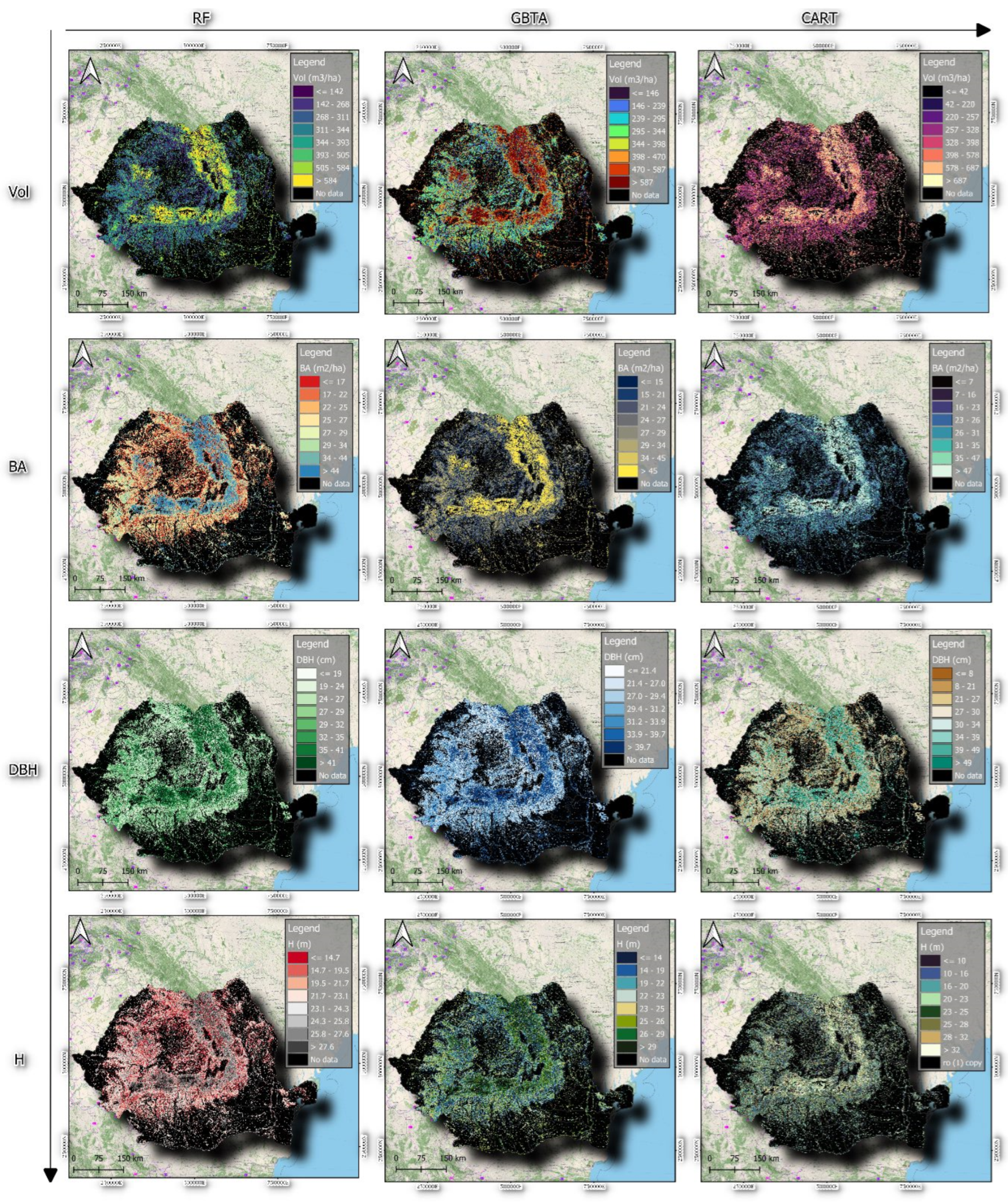
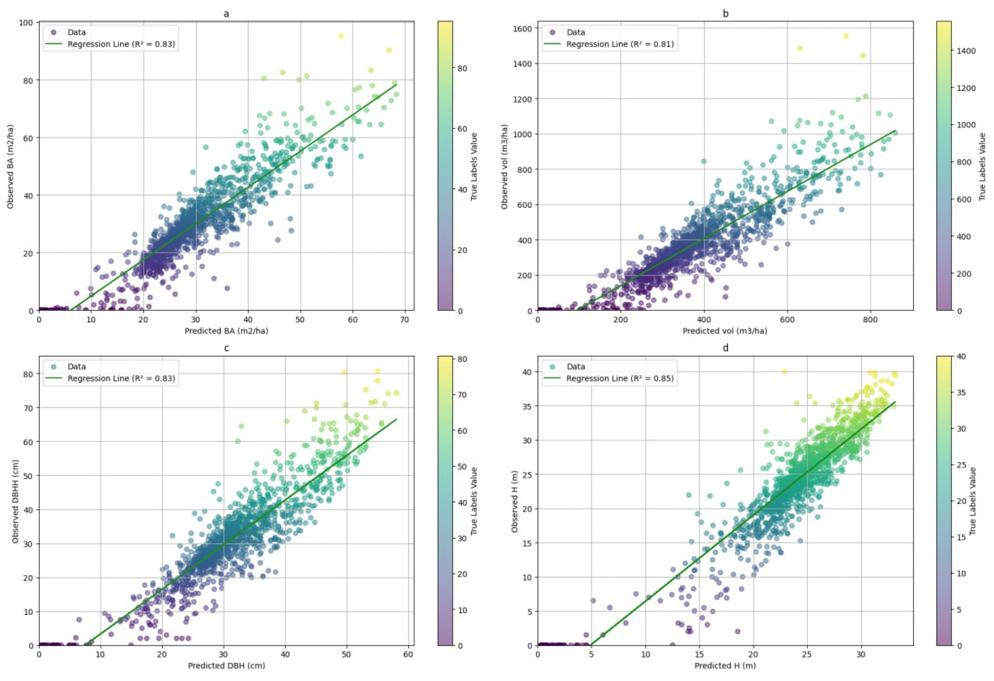
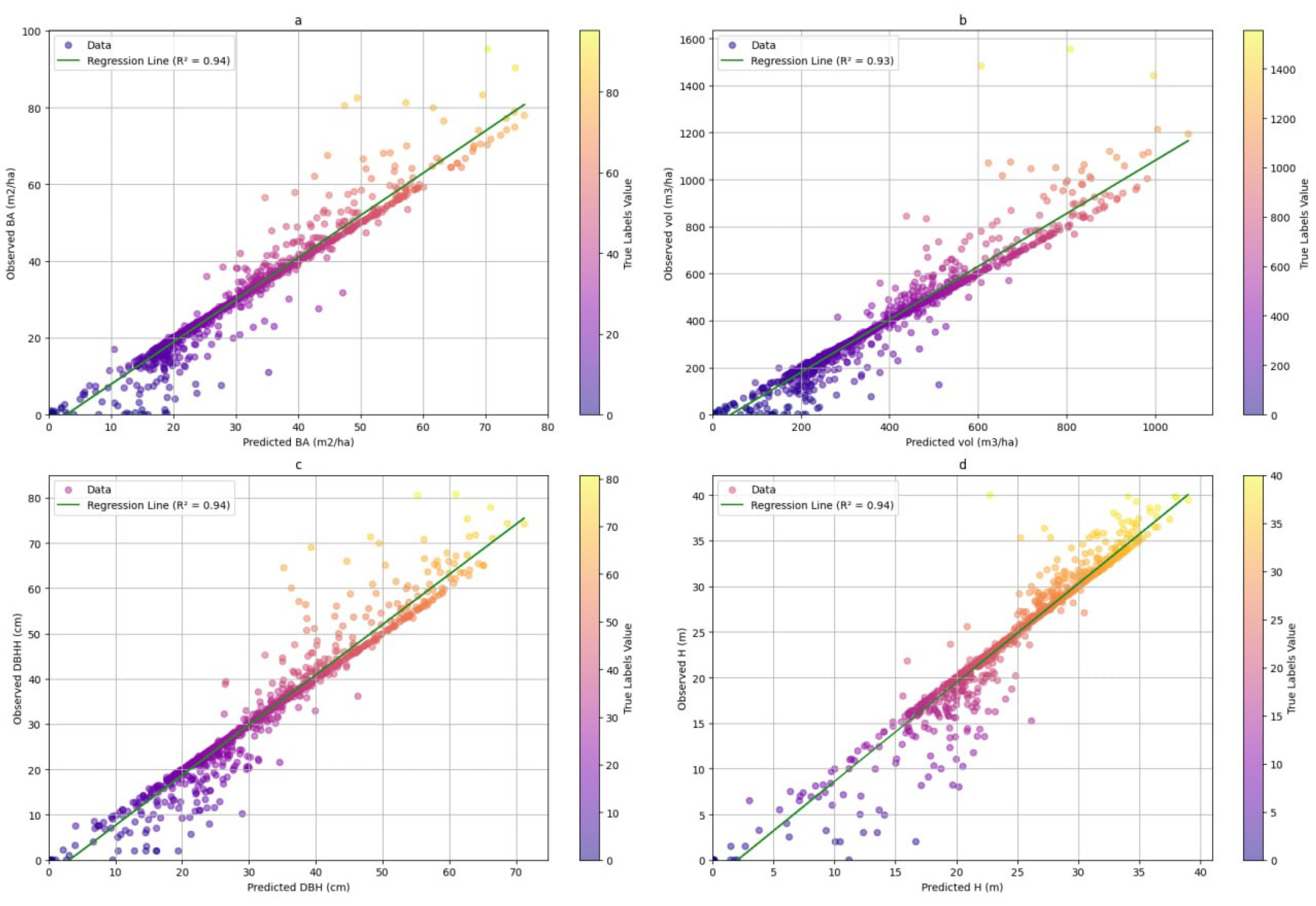
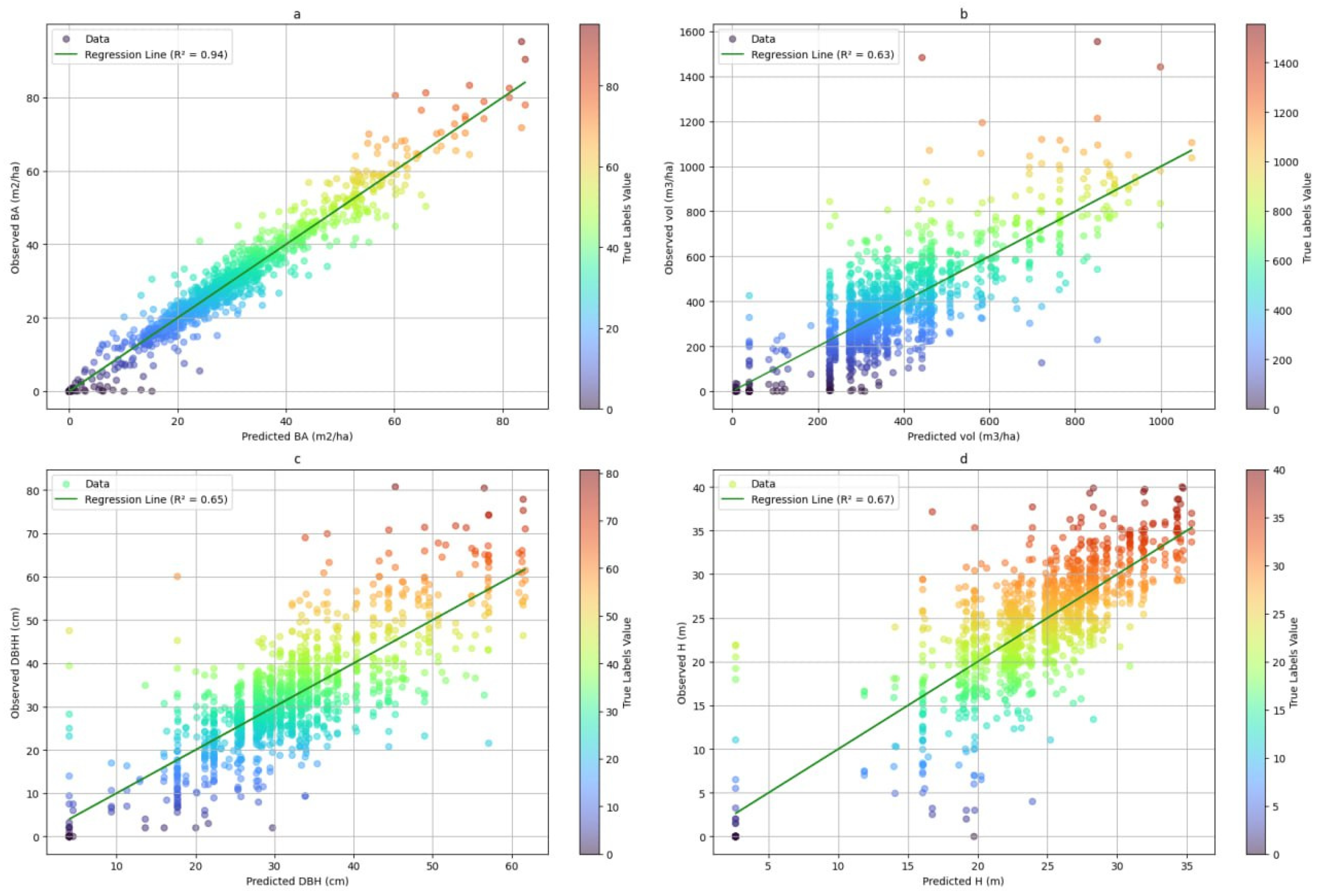

Table 1.
Performance of machine learning algorithms in the validation datasets attributes and scenarios.
Table 1.
Performance of machine learning algorithms in the validation datasets attributes and scenarios.
| Attribute | Model | N0 of trees | RMSE | MAE | rRMSE(%) | R2 |
| Vol (m3/ha) |
RF | 100 | 107.461 | -2.420 | 0.284 | 0.810 |
| 1000 | 107.727 | -1.217 | 0.285 | 0.810 | ||
| 3500 | 107.643 | -1.013 | 0.285 | 0.810 | ||
| GBTA | 100 | 178.085 | 17.077 | 0.471 | 0.660 | |
| 1000 | 89.769 | 2.105 | 0.237 | 0.860 | ||
| 2500 | 64.507 | 1.499 | 0.171 | 0.930 | ||
| CART | 1000 | 132.663 | 0.000 | 0.351 | 0.630 | |
| BA (m2/ha) |
RF | 100 | 6.617 | -0.020 | 0.223 | 0.830 |
| 1000 | 6.594 | -0.047 | 0.222 | 0.830 | ||
| 3500 | 6.585 | -0.046 | 0.222 | 0.830 | ||
| GBTA | 100 | 11.520 | 1.039 | 0.388 | 0.710 | |
| 1000 | 5.286 | -0.177 | 0.178 | 0.889 | ||
| 2500 | 3.809 | -0.113 | 0.128 | 0.940 | ||
| CART | 1000 | 3.564 | 0.000 | 0.120 | 0.941 | |
| DBH (cm) | RF | 100 | 6.402 | -0.005 | 0.205 | 0.816 |
| 1000 | 6.311 | -0.029 | 0.202 | 0.826 | ||
| 3500 | 6.294 | -0.034 | 0.201 | 0.827 | ||
| GBTA | 100 | 10.768 | 0.923 | 0.345 | 0.708 | |
| 1000 | 5.154 | -0.061 | 0.165 | 0.874 | ||
| 2500 | 3.616 | 3.616 | -0.044 | 0.936 | ||
| CART | 1000 | 7.904 | 0.000 | 0.253 | 0.653 | |
| H (m) | RF | 100 | 3.207 | -0.022 | 0.135 | 0.839 |
| 1000 | 3.198 | -0.009 | 0.134 | 0.845 | ||
| 3500 | 3.192 | -0.014 | 0.134 | 0.845 | ||
| GBTA | 100 | 2.589 | -0.290 | 0.109 | 0.750 | |
| 1000 | 2.589 | -0.290 | 0.109 | 0.891 | ||
| 2500 | 1.868 | -0.199 | 0.078 | 0.941 | ||
| CART | 1000 | 4.234 | 0.000 | 0.178 | 0.665 |
Figure 3.
Forest characteristics modelling results at national level.
Figure 4.
Scatterplots for the RF regression model of forest stand attributes: (a) basal area (b) tree volume (Vol) (c) diameter at breast height (DBH) (d) tree height (H).
Figure 4.
Scatterplots for the RF regression model of forest stand attributes: (a) basal area (b) tree volume (Vol) (c) diameter at breast height (DBH) (d) tree height (H).
Figure 5.
Scatterplots for the GBTA regression model of forest stand attributes: (a) basal area (b) tree volume (Vol) (c) diameter at breast height (DBH) (d) tree height (H).
Figure 5.
Scatterplots for the GBTA regression model of forest stand attributes: (a) basal area (b) tree volume (Vol) (c) diameter at breast height (DBH) (d) tree height (H).
Figure 6.
Scatterplots for the CART regression model of forest attributes: (a) basal area (b) tree volume (Vol) (c) diameter at breast height (DBH) (d) tree height (H).
Figure 6.
Scatterplots for the CART regression model of forest attributes: (a) basal area (b) tree volume (Vol) (c) diameter at breast height (DBH) (d) tree height (H).
3.2. Model Performance Assessment with Independent Validation Data in the Test Area
The assessment of prediction accuracy and reliability through comparison with independent ground truth data in Lempes test area indicates that, RF and GBTA algorithms with a maximum number of suggested trees demonstrated high performance in predicting various forest attributes during the evaluation with initial validation data. The CART algorithm exhibited reliable outcomes specifically in predicting BA. Based on these findings, these three models were selected for further analysis. This selection process was crucial to ensure the robustness and generalizability of the chosen models.
3.2.1. Visual Assessment of the Models in Mapping Forest Characteristics
The detailed maps presented in Figure 7, Figure 8, Figure 9 and Figure 10 illustrate the predictive modelling of forest attributes across the entire test area. These intricate cartographic representations provide a granular perspective on model predictions at a spatial resolution of 10 meters. The three models show varying degrees of accuracy in their estimations compared to observed data.
GBTA consistently provides predictions that closely align with the actual data, particularly excelling in capturing the upper range of values such as taller tree heights, larger DBH, higher volumes, and BA. RF generally achieves accuracy comparable to GBTA but tends to produce more moderate predictions. It often smooths out extremes and may slightly underpredict in areas with exceptionally large trees. CART, on the other hand, tends to underpredict, especially in regions with higher observed values, showing a more conservative approach, particularly in predicting larger trees in terms of H, DBH, and Vol. Overall, GBTA is the most accurate visually for environments with high variability, RF offers reliable but more moderate predictions, and CART is best suited for scenarios where lower, conservative estimates are preferable.
3.2.2. Evaluation of Predictive Accuracy in Forest Attribute Estimation Across Different Resolutions
The accuracy of these algorithms in predicting the independent dataset, when varying the pixel size from low to high are presented in Table 3. This comprehensive assessment allowed an optimal determination of the balance between detail and precision for optimal prediction.
At the 10-meter resolution, the accuracy of the models is generally low. This finer resolution tends to introduce more variability and noise into the data, which the models struggle to handle effectively. Consequently, the coefficient of determination values are lower, suggesting that the models account for less variance in the data. Furthermore, the error metrics are higher, indicating reduced predictive performance.
When examining DBH and H, both RF and GBTA algorithms demonstrate significant improvement in R2 at 100 meters (about 55% the dataset was accurately predicted) with the lowest RMSE and rRMSE values, suggesting that higher pixel sizes lead to better predictive accuracy for these attributes. The CART algorithm follows a similar trend, with the best performance observed at 100 meters for both DBH and Height with 41.7%. This proves that for predicting DBH and Height, higher resolutions (100 meters) generally provide more accurate and precise results across all three algorithms, particularly for RF and GBTA.
For Vol, the RF and CART algorithm shows slight improvement in R2 at 100 meters, but this comes with significantly higher RMSE and rRMSE. In contrast, the GBTA algorithm demonstrates superior performance, with notable improvements in accuracy and decreasing errors at both 50-meter and 100-meter resolutions. For BA, the optimal accuracy and precision was at 50 m resolution for RF and GBTA algorithm, with a significant improvement in error metrics. The CART algorithm performs best at 10 meters but shows a decline in accuracy at higher resolutions. This indicates that the models struggle particularly with predicting Vol and BA effectively even when considering larger resolution.
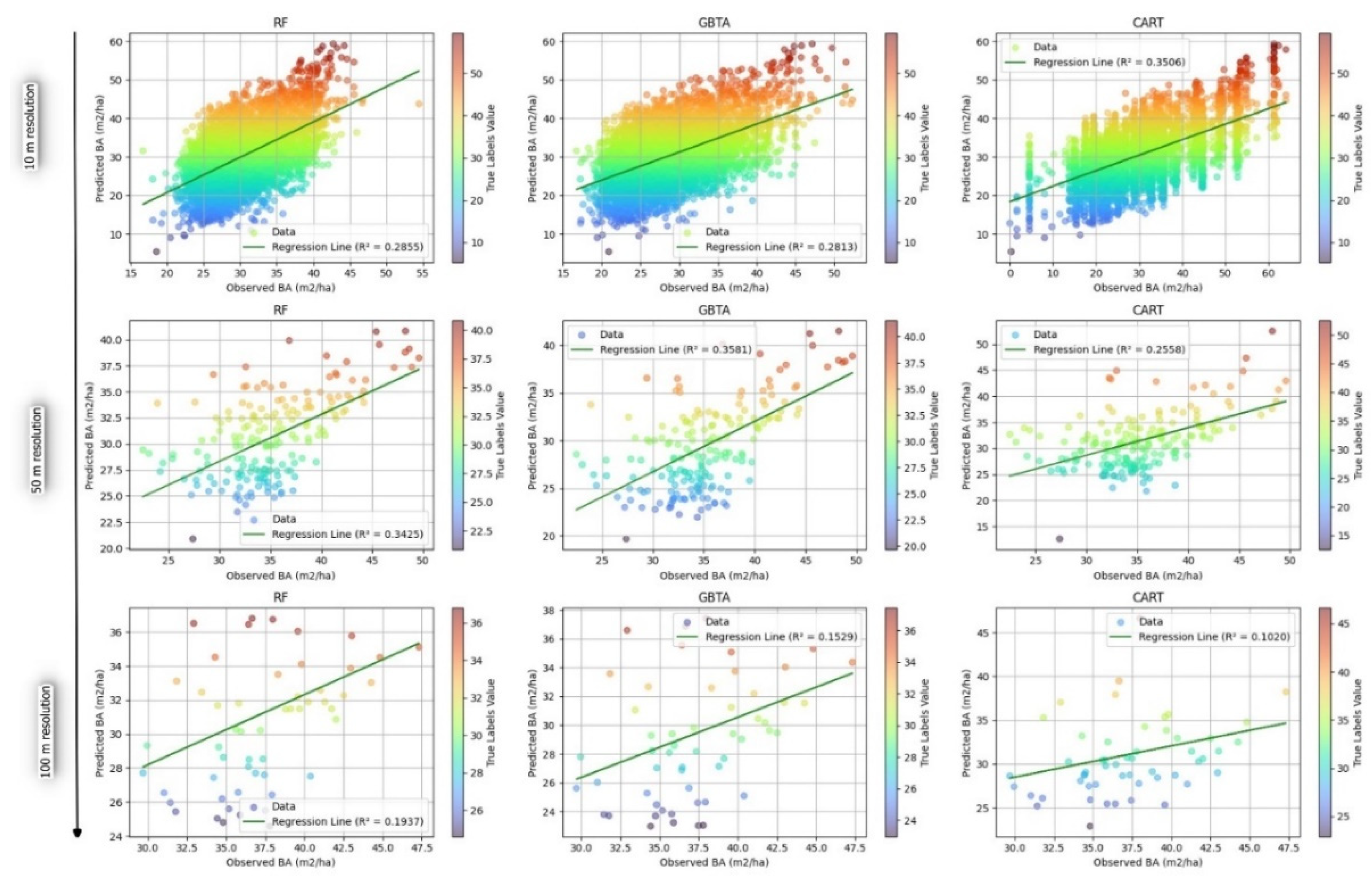
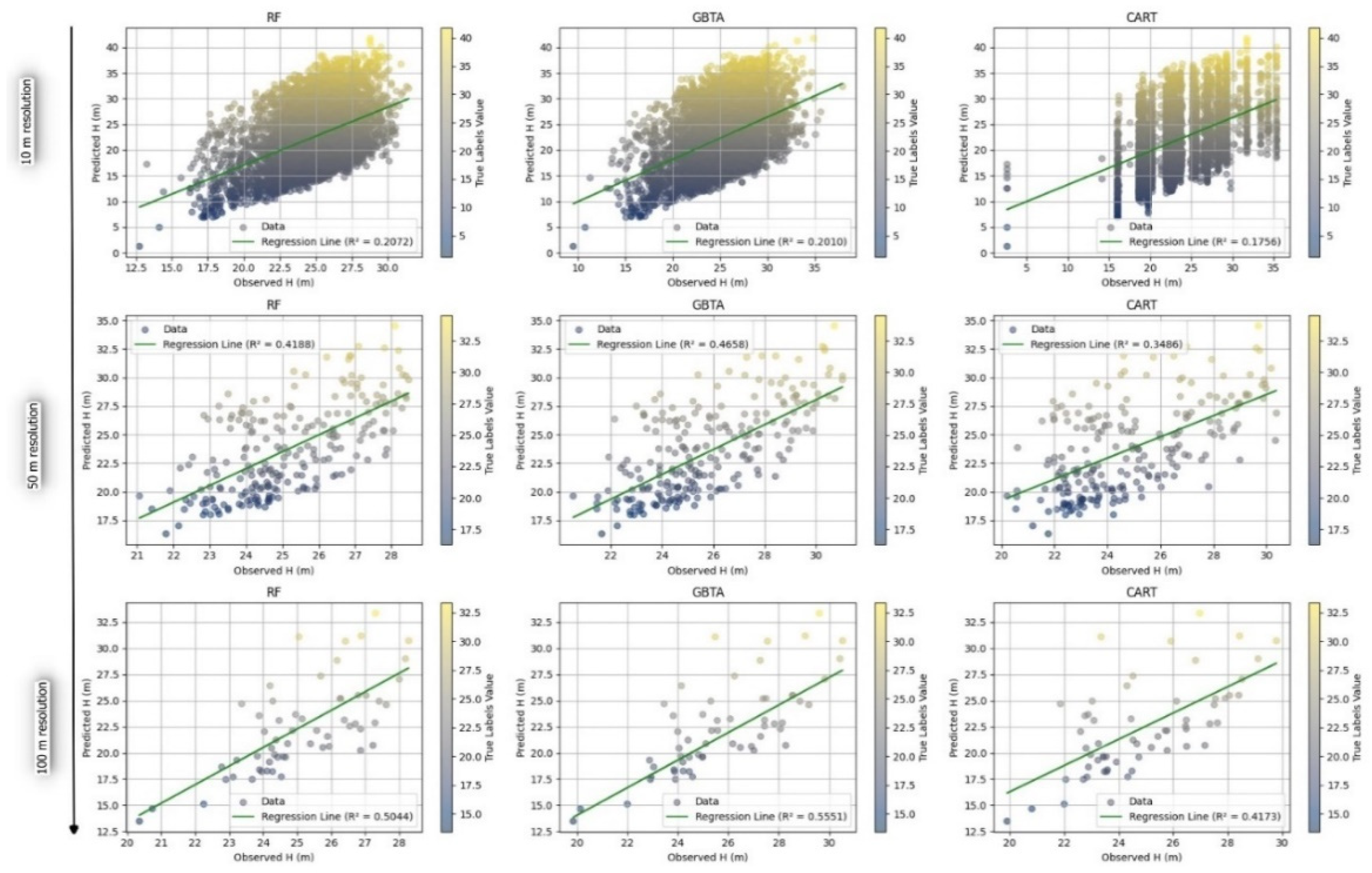
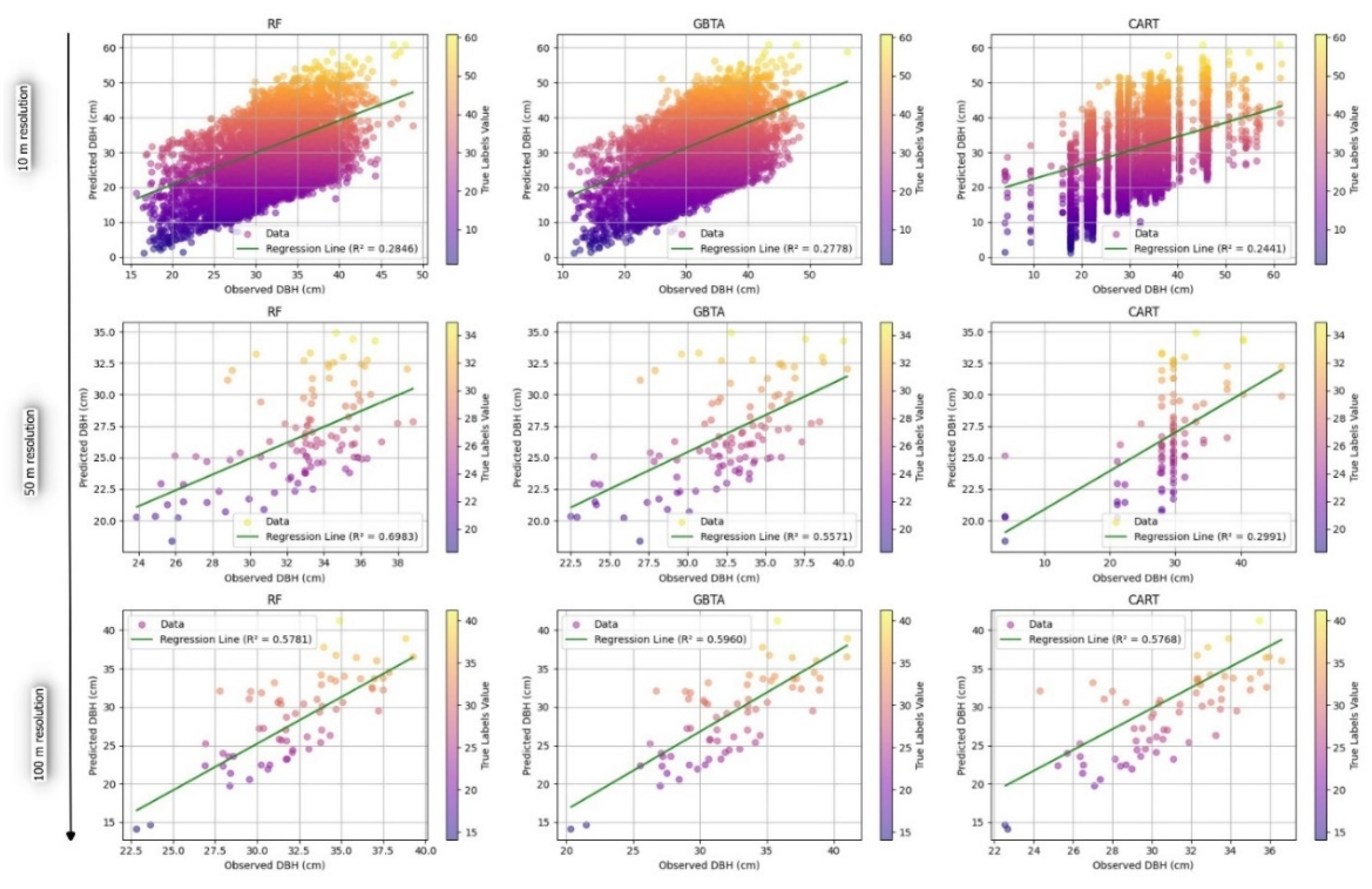
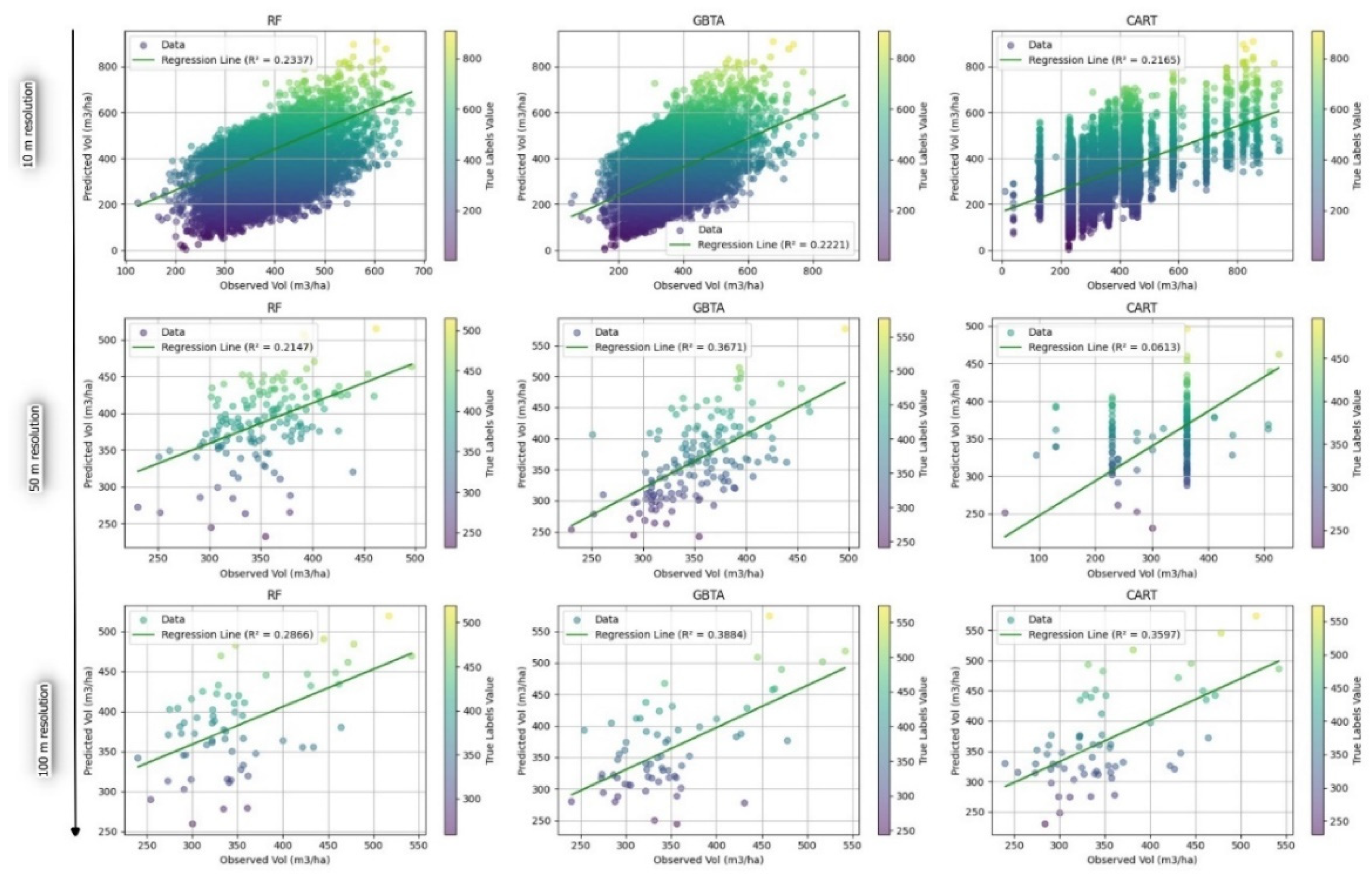
Figure 11.
Scatterplots for the models’ performance with the test area for BA prediction under different resolution.
Figure 11.
Scatterplots for the models’ performance with the test area for BA prediction under different resolution.
Figure 12.
Scatterplots for the models’ performance with the test area for H prediction under different resolution.
Figure 12.
Scatterplots for the models’ performance with the test area for H prediction under different resolution.
Figure 13.
Scatterplots for the models’ performance with the test area for DBH prediction under different resolution.
Figure 13.
Scatterplots for the models’ performance with the test area for DBH prediction under different resolution.
Figure 14.
Scatterplots for the models’ performance with the test area for Vol prediction under different resolution.
Figure 14.
Scatterplots for the models’ performance with the test area for Vol prediction under different resolution.
4. Discussion
Forests are essential ecosystems that sustain biodiversity, regulate climate, and provide critical resources such as timber and carbon sequestration capabilities. The increasing demand for sustainable forest management requires efficient and scalable tools for monitoring key forest attributes, including basal area (BA), standing stock volume (Vol), diameter at breast height (DBH), and tree height (H). Traditional ground-based measurements, while accurate, are resource-intensive and often impractical for large-scale assessments. This study leverages remote sensing technologies and machine learning (ML) algorithms—Random Forest (RF), Gradient Boosting Tree Algorithm (GBTA), and Classification and Regression Trees (CART)—to address these limitations, offering a modern, scalable solution for predicting forest attributes in Romania's diverse temperate forest ecosystems.
The main objectives were to evaluate the performance of these ML algorithms in predicting key forest attributes, assess the impact of model complexity on predictive accuracy, and determine the optimal spatial resolution for modeling fine-scale forest characteristics. These objectives align with the overarching goal of enhancing forest management practices globally by providing detailed and accurate forest attribute maps.
4.1. Comparative Algorithm Performance
The study revealed notable differences in the performance of RF, GBTA, and CART across various forest attributes. GBTA emerged as the most robust algorithm, particularly for complex and variable attributes such as Vol and BA. At its optimal complexity (2,500 trees), GBTA achieved an R² of 0.92 for standing volume, outperforming other algorithms in terms of both accuracy and error metrics. This aligns with findings from similar studies where GBTA was favored for its ability to model intricate relationships in forest ecosystems [43,72,73].
RF demonstrated strong performance, explaining over 80% of the variance for most attributes, making it a reliable choice for large-scale applications. However, its tendency to underpredict in areas with extreme values was observed, as reported in prior studies [34,68]. The algorithm's moderate computational requirements and robustness to overfitting underscore its practicality for forest management applications.
CART, known for its interpretability, performed best in BA prediction, achieving the lowest RMSE values. Nevertheless, its conservative predictions for attributes such as DBH and H highlight its limitations in handling complex, nonlinear relationships. This corroborates findings from studies suggesting CART’s suitability for scenarios requiring simple and transparent decision-making frameworks [38,39].
4.2. Influence of Model Complexity and Impact of Spatial Resolution
A key objective of this study was to assess whether increased model complexity enhances predictive accuracy. Results confirmed that while higher complexity generally improved performance, diminishing returns were observed beyond a certain threshold. For instance, GBTA's accuracy plateaued as tree numbers exceeded 2,500, emphasizing the importance of balanced hyperparameter optimization. These findings align with previous research, which highlights the trade-offs between model complexity and overfitting risks [25].
RF displayed resilience to overfitting, achieving consistent accuracy across different complexity levels. This characteristic makes it particularly valuable for large-scale forest assessments, where overfitting poses a significant challenge [35,36]. In contrast, CART exhibited greater sensitivity to model complexity, reinforcing its role as a simpler yet less flexible algorithm for specific applications.
The impact of spatial resolution on model performance was a pivotal focus of this study. Fine resolutions (10 m) captured detailed variability but introduced noise, reducing predictive accuracy. Intermediate resolutions (50 m) offered a balance between spatial detail and model performance, proving optimal for attributes like BA and H. Coarser resolutions (100 m) improved the accuracy of DBH predictions but sacrificed detail, particularly in heterogeneous landscapes.
These findings are consistent with studies that emphasize the trade-offs between resolution and accuracy in remote sensing applications [49,51]. The variability in optimal resolution across attributes underscores the need for tailored approaches based on specific management objectives. For instance, finer resolutions may be preferable for biodiversity assessments, while coarser resolutions may suffice for large-scale carbon stock estimation.
4.3. Broader Applicability of Results and Contributions to Forest Management
Romanian temperate forests, characterized by diverse species, management practices, and topographic conditions, serve as a representative case study for broader European and global contexts. The applicability of the results extends to other temperate forest ecosystems, where similar challenges in monitoring and managing forest attributes persist. The integration of Sentinel-2 data with ML algorithms offers a replicable framework for sustainable forest management across regions with varying ecological and management conditions.
The robust performance of GBTA and RF in this study aligns with global efforts to leverage machine learning for forest monitoring, highlighting their potential for scalable and accurate applications in diverse forest types [23,74]. Additionally, the adaptability of these algorithms to varying resolutions and attribute complexities enhances their utility for addressing regional and global forest management challenges.
By meeting the study's objectives, this research contributes significantly to the field of forest management. The ability to generate accurate, large-scale maps of forest attributes supports decision-making processes for timber harvesting, carbon accounting, and biodiversity conservation. The integration of advanced ML techniques with satellite data reduces the reliance on resource-intensive ground surveys, enabling cost-effective and scalable monitoring solutions.
The findings also emphasize the importance of selecting appropriate algorithms and resolutions based on management priorities. For example, GBTA is suitable for detailed assessments requiring high accuracy, while RF offers a practical alternative for broader applications. This flexibility ensures that forest managers can adapt these tools to specific needs, promoting efficient and sustainable resource management.
5. Conclusions
This study demonstrates the transformative potential of machine learning and remote sensing in forest management. By addressing the limitations of traditional methods, it provides a scalable, accurate, and efficient framework for monitoring forest attributes. The use of Romania’s forests as a representative case study highlights the global relevance of these findings, offering insights applicable to temperate forest ecosystems worldwide. Ultimately, the integration of advanced technologies into forest management practices represents a significant step toward achieving sustainability goals, balancing conservation and utilization to meet the needs of present and future generations.
Author Contributions
Conceptualization, MIK and MDN; methodology, MIK and MDN; software, MIK; validation, MIK, and AHM; formal analysis, SAB and MDN; investigation, MIK; resources, SAB and MDN; data curation, MIK and MDN; writing—original draft preparation, MIK, AHM and MDN; writing—review and editing, SAB and MDN; visualization, MIK; supervision, MDN; project administration, MDN; funding acquisition, SAB and MDN. All authors have read and agreed to the published version of the manuscript.
Funding
This research was funded by Transilvania University of Brasov.
Data Availability Statement
We encourage all authors of articles published in MDPI journals to share their research data. In this section, please provide details regarding where data supporting reported results can be found, including links to publicly archived datasets analyzed or generated during the study. Where no new data were created, or where data is unavailable due to privacy or ethical restrictions, a statement is still required. Suggested Data Availability Statements are available in section “MDPI Research Data Policies” at https://www.mdpi.com/ethics.
Acknowledgments
We are grateful to Forest Design Team in helping with the field data collection.
Conflicts of Interest
The authors declare no conflicts of interest.
Appendix A
Table A. Climate Characteristics of the test area (https://en.climate-data.org/).
Table A. Climate Characteristics of the test area (https://en.climate-data.org/).
| Characteristic | Description |
| Climate classification | Köppen-Geiger: Dfb |
| Average annual temperature | 7ºC |
| Warmest month | July |
| Coldest month | January |
| Annual precipitation | Approximately 794 mm (31.3 inches) |
| Monthly temperature variation | 22.7°C (40.8°F) |
| Month with highest humidity | January (80.11%) |
| Month with lowest humidity | August (69.98%) |
| Month with most rainy days | May (14.07 days) |
| Month with fewest rainy days | October (8.03 days) |
| Rainfall distribution | Even distribution throughout the year; 70% in warm season (April to September), 30% in cold season (October to March) |
| Potential evapotranspiration | 594 mm annually, 480 mm during warm period, 110 mm during cold period |
Table B. Hydrography and Soil Composition Characteristics.
| Category | Description |
| Hydrography | The hydrographic network is highly developed and rich in running waters, with frequent occurrences of springs due to the permanently high-water table. |
| Streams | The marsh area is crossed by streams including Husbor Brook, Brook under Coasta, and Morilor Valley. |
| Groundwater | Depths range from 30 to 56 meters, with a piezometric level situated at a depth of 2.7 meters. |
| Soil | The site area is covered by Hydrosols and alluvial soils, 100%. Hydrosols in the first 50 cm of soil form gleysols. Active peat, eutrophic peat about 1m thick, formed on a substrate of gravel and sand. Of the class of unevolved soils, truncated or deflated, there is also the type of alluvial soil. |
Table C. Descriptive statistics of the national scale dataset used for machine learning.
| Stastic | BA (m2/ha) | DBH (cm) | H (m) | Vol (m3/ha) |
| Mean | 30.554 | 32.195 | 24.564 | 389.643 |
| Standard Error | 0.388 | 0.347 | 0.171 | 5.921 |
| Median | 28.296 | 30.100 | 25.100 | 359.864 |
| Mode | 26.800 | 28.000 | 20.000 | 375.900 |
| Standard Deviation | 13.929 | 12.446 | 6.118 | 212.330 |
| Range | 95.180 | 79.738 | 38.500 | 1554.389 |
| Minimum | 0.010 | 1.000 | 1.500 | 0.013 |
| Maximum | 95.190 | 80.738 | 40.000 | 1554.402 |
| 1st quartile | 22.100 | 25.360 | 21.440 | 253.381 |
| 3rd quartile | 36.413 | 37.590 | 28.260 | 480.499 |
| CV % | 45.589 | 38.659 | 24.908 | 54.494 |
Table D. Descriptive statistics of the independent dataset used to validate the national product in the test area.
Table D. Descriptive statistics of the independent dataset used to validate the national product in the test area.
| Statistic | BA (m2/ha) | DBH (cm) | H (m) | Vol (m3/ha) |
| Mean | 43.892 | 27.903 | 19.650 | 343.095 |
| Standard Error | 0.287 | 0.149 | 0.113 | 2.743 |
| Median | 41.188 | 27.513 | 19.197 | 315.663 |
| Mode | 43.800 | 31.300 | 22.700 | 269.850 |
| Standard Deviation | 16.791 | 8.727 | 6.589 | 160.335 |
| Range | 162.425 | 58.426 | 35.733 | 1723.700 |
| Minimum | 0.400 | 9.514 | 3.100 | 1.175 |
| Maximum | 162.825 | 67.940 | 38.833 | 1724.875 |
| 1st quartile | 33.300 | 21.914 | 14.800 | 244.844 |
| 3rd quartile | 51.180 | 32.762 | 24.150 | 404.219 |
| CV % | 38.256 | 31.277 | 33.532 | 46.732 |
Table E. Vegetation indices, band used, formula and description.
| Index | Bands Used | Formula | Description, Applications & Rationale |
| Normalized Difference Vegetation Index (NDVI) | NIR (B8) Red (B4) |
Measures vegetation health by comparing NIR reflectance (healthy vegetation) with Red reflectance (chlorophyll absorption). Chosen for its widespread use in assessing vegetation cover and health. |
|
| Shadow Index (SI) | Blue (B2) Green (B3) Red (B4) |
Custom index to detect shadowed areas in forests using visible bands. Selected to differentiate shadows from water and dark surfaces. | |
| Soil-Adjusted Vegetation Index (SAVI) | NIR (B8) Red (B4) |
Minimizes soil brightness influence, improving vegetation detection in areas with sparse cover. Useful for agricultural fields and degraded lands. | |
| Enhanced Vegetation Index (EVI) | Blue (B2) Red (B4) NIR (B8) |
Enhances sensitivity to dense vegetation, reducing soil and atmospheric effects. Effective in monitoring forest canopy health. | |
| Bare Soil Index (BI) | SWIR1 (B11) SWIR2 (B12) NIR (B8) |
Differentiates bare soil from vegetation, useful in detecting exposed soils and erosion-prone areas. Selected for monitoring land degradation. | |
| Normalized Difference Infrared Index (NDII) | IR (B8) NIR (B8) |
Assesses water content in vegetation. Chosen for its ability to monitor drought stress and moisture levels in forests. |
Figure A.
Distribution of plot clusters used for training.

References
- Franco, A.L.C.; Sobral, B.W.; Silva, A.L.C.; Wall, D.H. Amazonian Deforestation and Soil Biodiversity. Conservation Biology 2019, 33, 590–600. [Google Scholar] [CrossRef]
- Stăncioiu, P.T.; Niță, M.D.; Lazăr, G.E. Forestland Connectivity in Romania—Implications for Policy and Management. Land use policy 2018, 76, 487–499. [Google Scholar] [CrossRef]
- Munteanu, C.; Senf, C.; Nita, M.D.; Sabatini, F.M.; Oeser, J.; Seidl, R.; Kuemmerle, T. Using Historical Spy Satellite Photographs and Recent Remote Sensing Data to Identify High-conservation-value Forests. Conservation Biology 2022, 36, e13820. [Google Scholar] [CrossRef] [PubMed]
- Lausch, A.; Blaschke, T.; Haase, D.; Herzog, F.; Syrbe, R.-U.; Tischendorf, L.; Walz, U. Understanding and Quantifying Landscape Structure – A Review on Relevant Process Characteristics, Data Models and Landscape Metrics. Ecol Modell 2015, 295, 31–41. [Google Scholar] [CrossRef]
- Nagendra, H.; Rocchini, D.; Ghate, R. Beyond Parks as Monoliths: Spatially Differentiating Park-People Relationships in the Tadoba Andhari Tiger Reserve in India. Biol Conserv 2010, 143, 2900–2908. [Google Scholar] [CrossRef]
- Chave, J.; Réjou-Méchain, M.; Búrquez, A.; Chidumayo, E.; Colgan, M.S.; Delitti, W.B.C.; Duque, A.; Eid, T.; Fearnside, P.M.; Goodman, R.C.; et al. Improved Allometric Models to Estimate the Aboveground Biomass of Tropical Trees. Glob Chang Biol 2014, 20, 3177–3190. [Google Scholar] [CrossRef]
- García, M.; Riaño, D.; Chuvieco, E.; Danson, F.M. Estimating Biomass Carbon Stocks for a Mediterranean Forest in Central Spain Using LiDAR Height and Intensity Data. Remote Sens Environ 2010, 114, 816–830. [Google Scholar] [CrossRef]
- Rahlf, J.; Hauglin, M.; Astrup, R.; Breidenbach, J. Timber Volume Estimation Based on Airborne Laser Scanning — Comparing the Use of National Forest Inventory and Forest Management Inventory Data. Ann For Sci 2021, 78, 49. [Google Scholar] [CrossRef]
- Capalb, F.; Apostol, B.; Lorent, A.; Petrila, M.; Marcu, C.; Badea, N.O. Integration of Terrestrial Laser Scanning and Field Measurements Data for Tree Stem Volume Estimation: Exploring Parametric and Non-Parametric Modeling Approaches. Ann For Res 2024, 67, 77–94. [Google Scholar] [CrossRef]
- Le Toan, T.; Quegan, S.; Davidson, M.W.J.; Balzter, H.; Paillou, P.; Papathanassiou, K.; Plummer, S.; Rocca, F.; Saatchi, S.; Shugart, H.; et al. The BIOMASS Mission: Mapping Global Forest Biomass to Better Understand the Terrestrial Carbon Cycle. Remote Sens Environ 2011, 115, 2850–2860. [Google Scholar] [CrossRef]
- Naik, P.; Dalponte, M.; Bruzzone, L. Prediction of Forest Aboveground Biomass Using Multitemporal Multispectral Remote Sensing Data. Remote Sens (Basel) 2021, 13, 1282. [Google Scholar] [CrossRef]
- Solberg, S.; Astrup, R.; Breidenbach, J.; Nilsen, B.; Weydahl, D. Monitoring Spruce Volume and Biomass with InSAR Data from TanDEM-X. Remote Sens Environ 2013, 139, 60–67. [Google Scholar] [CrossRef]
- Buendia, C.; Tanabe, E.; Kranjc, K.; Baasansuren, A.; Fukuda, J.; Ngarize, M.; Osako, S.; Pyrozhenko, A. Efinement to the 2006 IPCC Guidelines for National Greenhouse Gas Inventories Task Force on National Greenhouse Gas Inventories; IPCC, Switzerland., 2019; ISBN 978-4-88788-232-4.
- Hiraishi, Takahiko. Revised Supplementary Methods and Good Practice Guidance Arising from the Kyoto Protocol; Intergovernmental Panel on Climate Change, 2014; ISBN 9789291691401.
- Valbuena, R. Forest Structure Indicators Based on Tree Size Inequality and Their Relationships to Airborne Laser Scanning. Dissertationes Forestales 2015, 2015. [Google Scholar] [CrossRef]
- Verkerk, P.J.; Levers, C.; Kuemmerle, T.; Lindner, M.; Valbuena, R.; Verburg, P.H.; Zudin, S. Mapping Wood Production in European Forests. For Ecol Manage 2015, 357, 228–238. [Google Scholar] [CrossRef]
- Wulder, M.A.; White, J.C.; Nelson, R.F.; Næsset, E.; Ørka, H.O.; Coops, N.C.; Hilker, T.; Bater, C.W.; Gobakken, T. Lidar Sampling for Large-Area Forest Characterization: A Review. Remote Sens Environ 2012, 121, 196–209. [Google Scholar] [CrossRef]
- Huang, R.; Zhu, J. Using Random Forest to Integrate Lidar Data and Hyperspectral Imagery for Land Cover Classification. 2013. [CrossRef]
- Huang, T.; Ou, G.; Wu, Y.; Zhang, X.; Liu, Z.; Xu, H.; Xu, X.; Wang, Z.; Xu, C. Estimating the Aboveground Biomass of Various Forest Types with High Heterogeneity at the Provincial Scale Based on Multi-Source Data. Remote Sens (Basel) 2023, 15, 3550. [Google Scholar] [CrossRef]
- Smith, A.M.; Capinha, C.; Kramer, A.M. Predicting Species Distributions with Environmental Time Series Data and Deep Learning. bioRxiv (Cold Spring Harbor Laboratory) 2022. [CrossRef]
- Jiang, F.; Smith, A.R.; Kutia, M.; Wang, G.; Liu, H.; Sun, H. A Modified KNN Method for Mapping the Leaf Area Index in Arid and Semi-Arid Areas of China. Remote Sens (Basel) 2020, 12, 1884. [Google Scholar] [CrossRef]
- Gidey, E.; Mhangara, P. An Application of Machine-Learning Model for Analyzing the Impact of Land-Use Change on Surface Water Resources in Gauteng Province, South Africa. Remote Sens (Basel) 2023, 15, 4092. [Google Scholar] [CrossRef]
- Luo, Y.; Qi, S.; Liao, K.; Zhang, S.; Hu, B.; Tian, Y. Mapping the Forest Height by Fusion of ICESat-2 and Multi-Source Remote Sensing Imagery and Topographic Information: A Case Study in Jiangxi Province, China. Forests 2023, 14. [Google Scholar] [CrossRef]
- Ferraz, A.; Saatchi, S.S.; Longo, M.; Clark, D.B. Tropical Tree Size–Frequency Distributions from Airborne Lidar. Ecological Applications 2020, 30. [Google Scholar] [CrossRef]
- Nemeth, M.; Borkin, D.; Michalconok, G. The Comparison of Machine-Learning Methods XGBoost and LightGBM to Predict Energy Development. Computational Statistics and Mathematical Modeling Methods in Intelligent Systems 2019, 208–215. [Google Scholar] [CrossRef]
- Burzykowski, T.; Geubbelmans, M.; Rousseau, A.-J.; Valkenborg, D. Validation of Machine Learning Algorithms. American Journal of Orthodontics and Dentofacial Orthopedics 2023, 164, 295–297. [Google Scholar] [CrossRef] [PubMed]
- Ghosh, S.M.; Behera, M.D.; Paramanik, S. Canopy Height Estimation Using Sentinel Series Images through Machine Learning Models in a Mangrove Forest. Remote Sens (Basel) 2020, 12, 1519. [Google Scholar] [CrossRef]
- Breiman, L. Random Forests. Mach Learn 2001, 45, 5–32. [Google Scholar] [CrossRef]
- Tang, Z.; Xia, X.; Huang, Y.; Lu, Y.; Guo, Z. Estimation of National Forest Aboveground Biomass from Multi-Source Remotely Sensed Dataset with Machine Learning Algorithms in China. Remote Sens (Basel) 2022, 14, 5487. [Google Scholar] [CrossRef]
- Chen, M.; Qiu, X.; Zeng, W.; Peng, D. Combining Sample Plot Stratification and Machine Learning Algorithms to Improve Forest Aboveground Carbon Density Estimation in Northeast China Using Airborne LiDAR Data. Remote Sens (Basel) 2022, 14, 1477. [Google Scholar] [CrossRef]
- Li, C.; Zhou, L.; Xu, W. Estimating Aboveground Biomass Using Sentinel-2 MSI Data and Ensemble Algorithms for Grassland in the Shengjin Lake Wetland, China. Remote Sens (Basel) 2021, 13, 1595. [Google Scholar] [CrossRef]
- Ghosh, S.M.; Behera, M.D.; Kumar, S.; Das, P.; Prakash, A.J.; Bhaskaran, P.K.; Roy, P.S.; Barik, S.K.; Jeganathan, C.; Srivastava, P.K.; et al. Predicting the Forest Canopy Height from LiDAR and Multi-Sensor Data Using Machine Learning over India. Remote Sens (Basel) 2022, 14, 5968. [Google Scholar] [CrossRef]
- Hu, T.; Sun, Y.; Jia, W.; Li, D.; Zou, M.; Zhang, M. Study on the Estimation of Forest Volume Based on Multi-Source Data. Sensors 2021, 21, 7796. [Google Scholar] [CrossRef]
- McRoberts, R.E. A Two-Step Nearest Neighbors Algorithm Using Satellite Imagery for Predicting Forest Structure within Species Composition Classes. Remote Sens Environ 2009, 113, 532–545. [Google Scholar] [CrossRef]
- Cutler, D.R.; Edwards, T.C.; Beard, K.H.; Cutler, A.; Hess, K.T.; Gibson, J.; Lawler, J.J. RANDOM FORESTS FOR CLASSIFICATION IN ECOLOGY. Ecology 2007, 88, 2783–2792. [Google Scholar] [CrossRef] [PubMed]
- Witten, I.H.; Frank, E.; Hall, M.A. Data Mining: Practical Machine Learning Tools and Techniques; Elsevier, 2010; ISBN 9780123748560.
- Jeong, J.H.; Resop, J.P.; Mueller, N.D.; Fleisher, D.H.; Yun, K.; Butler, E.E.; Timlin, D.J.; Shim, K.-M.; Gerber, J.S.; Reddy, V.R.; et al. Random Forests for Global and Regional Crop Yield Predictions. PLoS One 2016, 11, e0156571–e0156571. [Google Scholar] [CrossRef] [PubMed]
- Mola, F.; Miele, R. Evolutionary Algorithms for Classification and Regression Trees. Data Analysis, Classification and the Forward Search 2006, 255–262, doi:10.1007/3-540-35978-8_29. [CrossRef]
- Salzberg, S.L. Book Review: C4.5: Programs for Machine Learning by J. Ross Quinlan. Morgan Kaufmann Publishers, Inc., 1993. Mach Learn 1994, 16, 235–240. [Google Scholar] [CrossRef]
- Franklin, J. The Elements of Statistical Learning: Data Mining, Inference and Prediction. The Mathematical Intelligencer 2005, 27, 83–85. [Google Scholar] [CrossRef]
- Zhang, N.; Chen, M.; Yang, F.; Yang, C.; Yang, P.; Gao, Y.; Shang, Y.; Peng, D. Forest Height Mapping Using Feature Selection and Machine Learning by Integrating Multi-Source Satellite Data in Baoding City, North China. Remote Sens (Basel) 2022, 14, 4434. [Google Scholar] [CrossRef]
- Sprangers, O.; Schelter, S.; de Rijke, M. Probabilistic Gradient Boosting Machines for Large-Scale Probabilistic Regression. 2021. [CrossRef]
- Zhang, N.; Chen, M.; Yang, F.; Yang, C.; Yang, P.; Gao, Y.; Shang, Y.; Peng, D. Forest Height Mapping Using Feature Selection and Machine Learning by Integrating Multi-Source Satellite Data in Baoding City, North China. Remote Sens (Basel) 2022, 14, 4434. [Google Scholar] [CrossRef]
- Chirici, G.; Barbati, A.; Corona, P.; Marchetti, M.; Travaglini, D.; Maselli, F.; Bertini, R. Non-Parametric and Parametric Methods Using Satellite Images for Estimating Growing Stock Volume in Alpine and Mediterranean Forest Ecosystems. Remote Sens Environ 2008, 112, 2686–2700. [Google Scholar] [CrossRef]
- Vafaei, S.; Soosani, J.; Adeli, K.; Fadaei, H.; Naghavi, H.; Pham, T.; Tien Bui, D. Improving Accuracy Estimation of Forest Aboveground Biomass Based on Incorporation of ALOS-2 PALSAR-2 and Sentinel-2A Imagery and Machine Learning: A Case Study of the Hyrcanian Forest Area (Iran). Remote Sens (Basel) 2018, 10, 172. [Google Scholar] [CrossRef]
- Peng, X.; Zhao, A.; Chen, Y.; Chen, Q.; Liu, H.; Wang, J.; Li, H. Comparison of Modeling Algorithms for Forest Canopy Structures Based on UAV-LiDAR: A Case Study in Tropical China. Forests 2020, 11, 1324. [Google Scholar] [CrossRef]
- Rubbens, P.; Brodie, S.; Cordier, T.; Destro Barcellos, D.; Devos, P.; Fernandes-Salvador, J.A.; Fincham, J.I.; Gomes, A.; Handegard, N.O.; Howell, K.; et al. Machine Learning in Marine Ecology: An Overview of Techniques and Applications. ICES Journal of Marine Science 2023, 80, 1829–1853. [Google Scholar] [CrossRef]
- Stăncioiu, P.T.; Niță, M.D.; Fedorca, M. Capercaillie (Tetrao Urogallus) Habitat in Romania A Landscape Perspective Revealed by Cold War Spy Satellite Images. Science of The Total Environment 2021, 781, 146763. [Google Scholar] [CrossRef]
- Saha, T.K.; Pal, S.; Talukdar, S.; Debanshi, S.; Khatun, R.; Singha, P.; Mandal, I. How Far Spatial Resolution Affects the Ensemble Machine Learning Based Flood Susceptibility Prediction in Data Sparse Region. J Environ Manage 2021, 297, 113344. [Google Scholar] [CrossRef] [PubMed]
- Munteanu, C.; Kuemmerle, T.; Boltiziar, M.; Butsic, V.; Gimmi, U.; Kaim, D.; Király, G.; Konkoly-Gyuró, É.; Kozak, J.; Lieskovský, J.; et al. Forest and Agricultural Land Change in the Carpathian Region—A Meta-Analysis of Long-Term Patterns and Drivers of Change. Land use policy 2014, 38, 685–697. [Google Scholar] [CrossRef]
- Cracknell, M.J.; Reading, A.M. Geological Mapping Using Remote Sensing Data: A Comparison of Five Machine Learning Algorithms, Their Response to Variations in the Spatial Distribution of Training Data and the Use of Explicit Spatial Information. Comput Geosci 2014, 63, 22–33. [Google Scholar] [CrossRef]
- Ota, T.; Ogawa, M.; Shimizu, K.; Kajisa, T.; Mizoue, N.; Yoshida, S.; Takao, G.; Hirata, Y.; Furuya, N.; Sano, T.; et al. Aboveground Biomass Estimation Using Structure from Motion Approach with Aerial Photographs in a Seasonal Tropical Forest. Forests 2015, 6. [Google Scholar] [CrossRef]
- Lang, N.; Schindler, K.; Wegner, J.D. Country-Wide High-Resolution Vegetation Height Mapping with Sentinel-2. Remote Sens Environ 2019, 233, 111347. [Google Scholar] [CrossRef]
- Silveira, E.M.O.; Radeloff, V.C.; Martinuzzi, S.; Martinez Pastur, G.J.; Bono, J.; Politi, N.; Lizarraga, L.; Rivera, L.O.; Ciuffoli, L.; Rosas, Y.M.; et al. Nationwide Native Forest Structure Maps for Argentina Based on Forest Inventory Data, SAR Sentinel-1 and Vegetation Metrics from Sentinel-2 Imagery. Remote Sens Environ 2023, 285, 113391. [Google Scholar] [CrossRef]
- Spârchez, G.; Târziu, D.R.; Dincă, L. Pedologie Cu Elemente de Geologie Și Geomorfologie. Editura Universității Transilvania din Brașov 2013.
- USGS Shuttle Radar Topography Mission Available online: http://www.landcover.org/data/srtm/.
- Nita, M.D.; Munteanu, C.; Gutman, G.; Abrudan, I.V.; Radeloff, V.C. Widespread Forest Cutting in the Aftermath of World War II Captured by Broad-Scale Historical Corona Spy Satellite Photography. Remote Sens Environ 2018, 204, 322–332. [Google Scholar] [CrossRef]
- García-Duro, J.; Ciceu, A.; Chivulescu, S.; Badea, O.; Tanase, M.A.; Aponte, C. Shifts in Forest Species Composition and Abundance under Climate Change Scenarios in Southern Carpathian Romanian Temperate Forests. Forests 2021, 12, 1434. [Google Scholar] [CrossRef]
- Munteanu, C.; Nita, M.D.; Abrudan, I.V.; Radeloff, V.C. Historical Forest Management in Romania Is Imposing Strong Legacies on Contemporary Forests and Their Management. For Ecol Manage 2016, 361, 179–193. [Google Scholar] [CrossRef]
- Niță, M.D. Testing Forestry Digital Twinning Workflow Based on Mobile LiDAR Scanner and AI Platform. Forests 2021, 12, 1576. [Google Scholar] [CrossRef]
- Giurgiu, V.; Decei, I.; Draghiciu, D. Metode Si Tabele Dendrometrice; Editura Ceres: Bucharest, 2004. [Google Scholar]
- Nguyen, Q.H.; Ly, H.B.; Ho, L.S.; Al-Ansari, N.; Van Le, H.; Tran, V.Q.; Prakash, I.; Pham, B.T. Influence of Data Splitting on Performance of Machine Learning Models in Prediction of Shear Strength of Soil. Math Probl Eng 2021, 2021. [Google Scholar] [CrossRef]
- Gorelick, N.; Hancher, M.; Dixon, M.; Ilyushchenko, S.; Thau, D.; Moore, R. Google Earth Engine: Planetary-Scale Geospatial Analysis for Everyone. Remote Sens Environ 2017, 202, 18–27. [Google Scholar] [CrossRef]
- Baban, G.; Daniel Niţă, M. Measuring Forest Height from Space. Opportunities and Limitations Observed in Natural Forests. Measurement 2023, 211, 112593. [Google Scholar] [CrossRef]
- Nita, M.-D.; Clinciu, I. Hydrological Mapping of the Vegetation Using Remote Sensing Products. Bulletin of the Transilvania University of Brasov, Series II. Forestry, Wood Industry, Agricultural Food Engineering 2010, 3.
- Potapov, P. V; Turubanova, S.A.; Tyukavina, A.; Krylov, A.M.; McCarty, J.L.; Radeloff, V.C.; Hansen, M.C. Eastern Europe’s Forest Cover Dynamics from 1985 to 2012 Quantified from the Full Landsat Archive. Remote Sens Environ 2015, 159, 28–43. [Google Scholar] [CrossRef]
- Friedman, J.H. Greedy Function Approximation: A Gradient Boosting Machine. The Annals of Statistics 2001, 29, 1189–1232. [Google Scholar] [CrossRef]
- Breiman, L. Random Forests. Mach Learn 2001, 45, 5–32. [Google Scholar] [CrossRef]
- Zhao, H.; Duan, S.; Liu, J.; Sun, L.; Reymondin, L. Evaluation of Five Deep Learning Models for Crop Type Mapping Using Sentinel-2 Time Series Images with Missing Information. Remote Sens (Basel) 2021, 13, 2790. [Google Scholar] [CrossRef]
- Montgomery, D. Design and Analysis of Experiments; John wiley & sons, 2017.
- Ilijević, K.; Obradović, M.; Jevremović, V.; Gržetić, I. Statistical Analysis of the Influence of Major Tributaries to the Eco-Chemical Status of the Danube River. Environ Monit Assess 2015, 187. [Google Scholar] [CrossRef]
- Chen, L.; Wang, Y.; Ren, C.; Zhang, B.; Wang, Z. Optimal Combination of Predictors and Algorithms for Forest Above-Ground Biomass Mapping from Sentinel and SRTM Data. Remote Sens (Basel) 2019, 11, 414. [Google Scholar] [CrossRef]
- Liu, J.; Zuo, Y.; Wang, N.; Yuan, F.; Zhu, X.; Zhang, L.; Zhang, J.; Sun, Y.; Guo, Z.; Guo, Y.; et al. Comparative Analysis of Two Machine Learning Algorithms in Predicting Site-Level Net Ecosystem Exchange in Major Biomes. Remote Sens (Basel) 2021, 13, 2242. [Google Scholar] [CrossRef]
- Jiang, F.; Smith, A.R.; Kutia, M.; Wang, G.; Liu, H.; Sun, H. A Modified KNN Method for Mapping the Leaf Area Index in Arid and Semi-Arid Areas of China. Remote Sens (Basel) 2020, 12, 1884. [Google Scholar] [CrossRef]
Figure 1.
Study area's geographic location: A) Romanian forests at continental scale B) Plots locations used at national scale C) Individual trees measurements used for independent validation in Lempes test area.
Figure 1.
Study area's geographic location: A) Romanian forests at continental scale B) Plots locations used at national scale C) Individual trees measurements used for independent validation in Lempes test area.
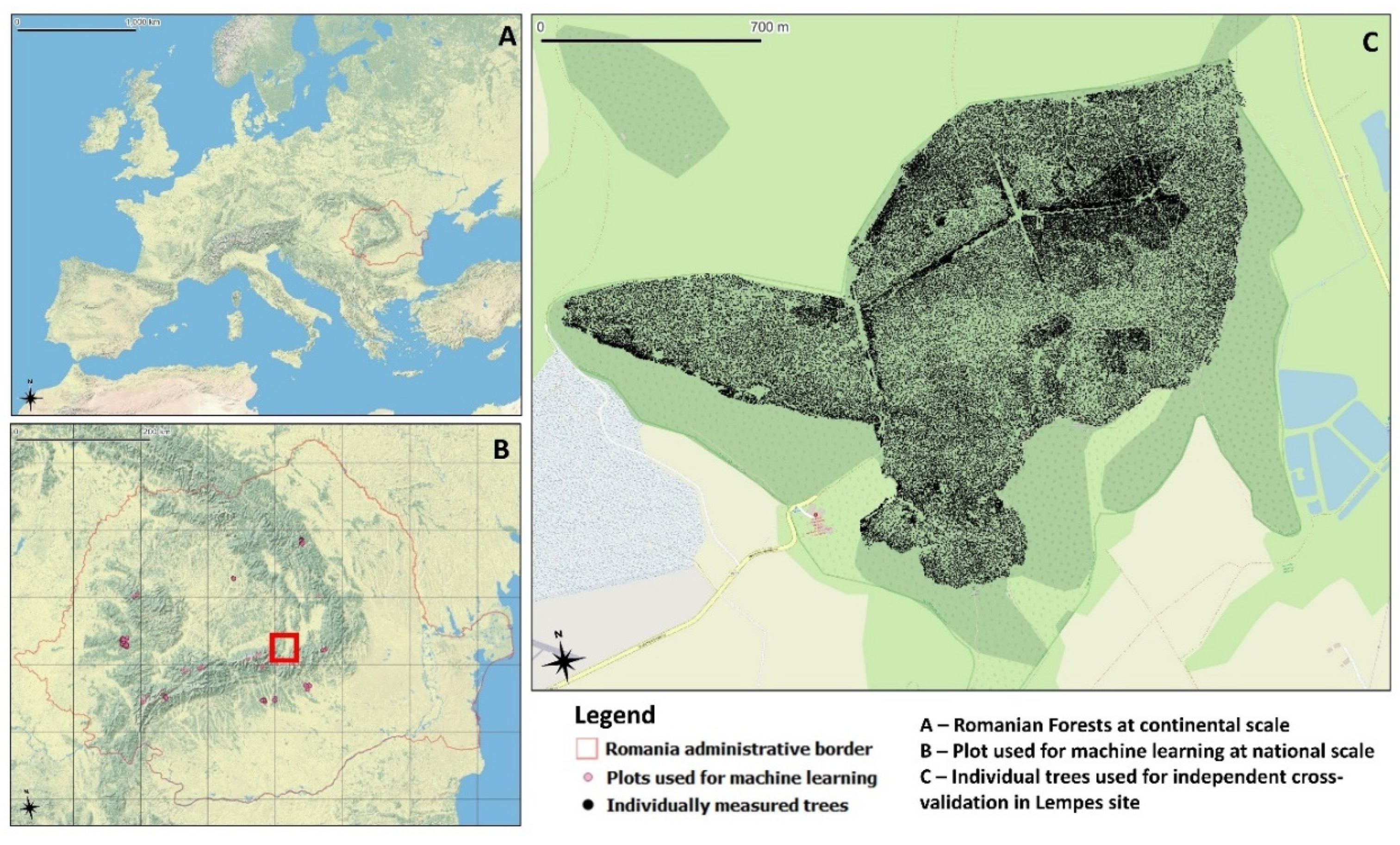
Figure 2.
Workflow diagram for data used in research.
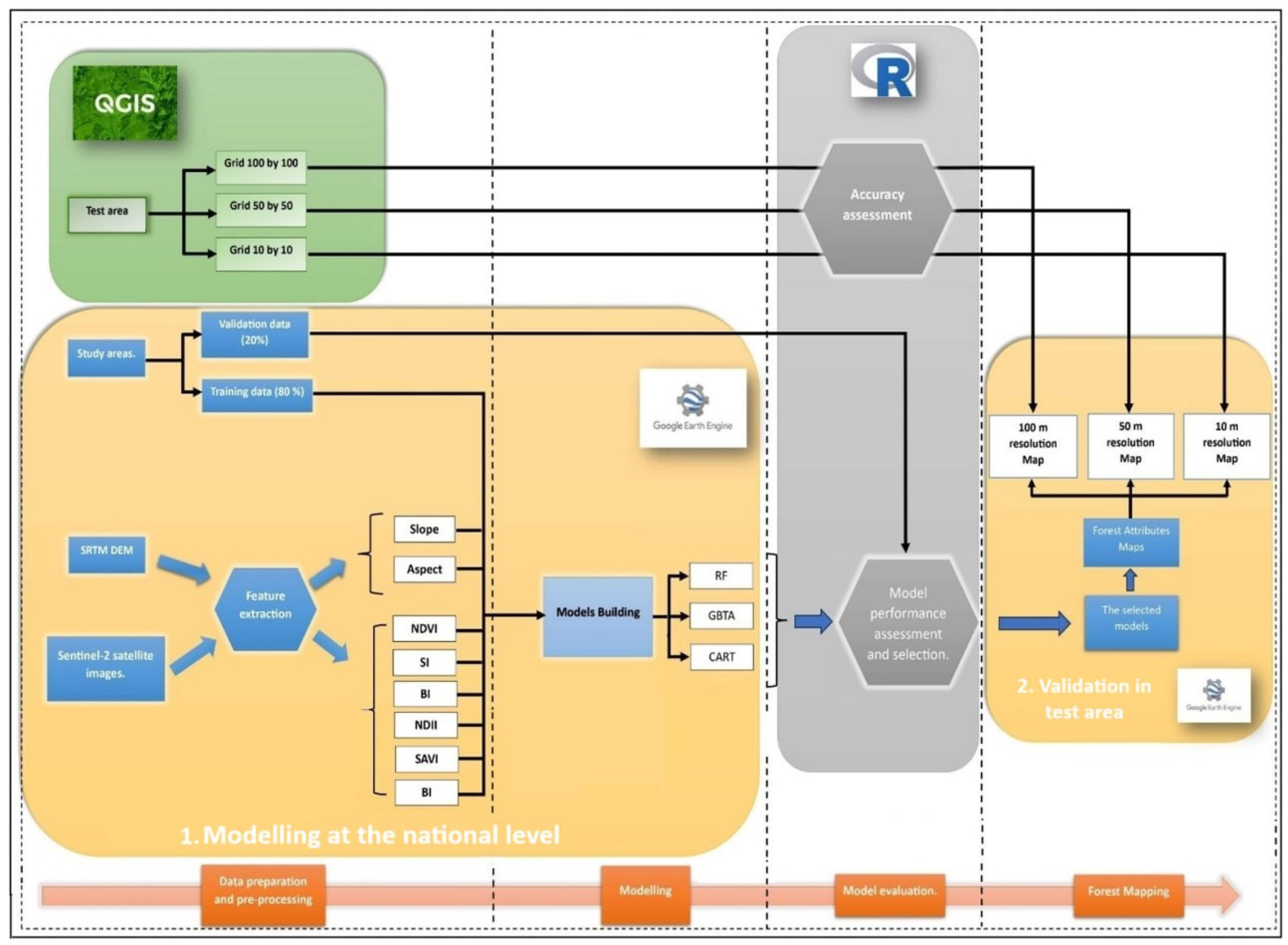
Figure 7.
Forest Characteristic Mapping for the BA using: (a) CART (b) RF (c) GTBA d) Field measurements.
Figure 7.
Forest Characteristic Mapping for the BA using: (a) CART (b) RF (c) GTBA d) Field measurements.
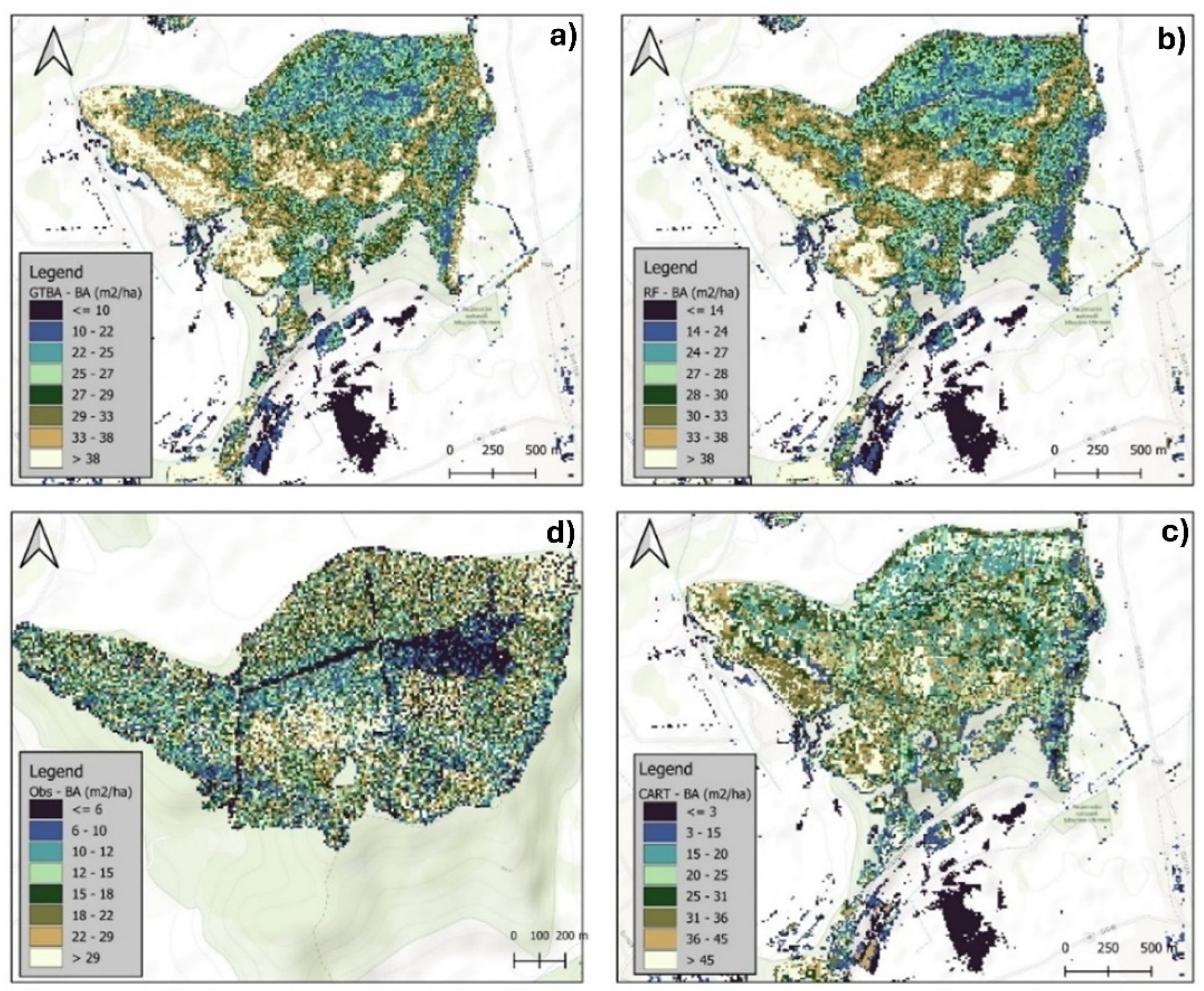
Figure 8.
Forest Characteristic Mapping for the Vol using: (a) CART (b) RF (c) GTBA d) Field measurements.
Figure 8.
Forest Characteristic Mapping for the Vol using: (a) CART (b) RF (c) GTBA d) Field measurements.
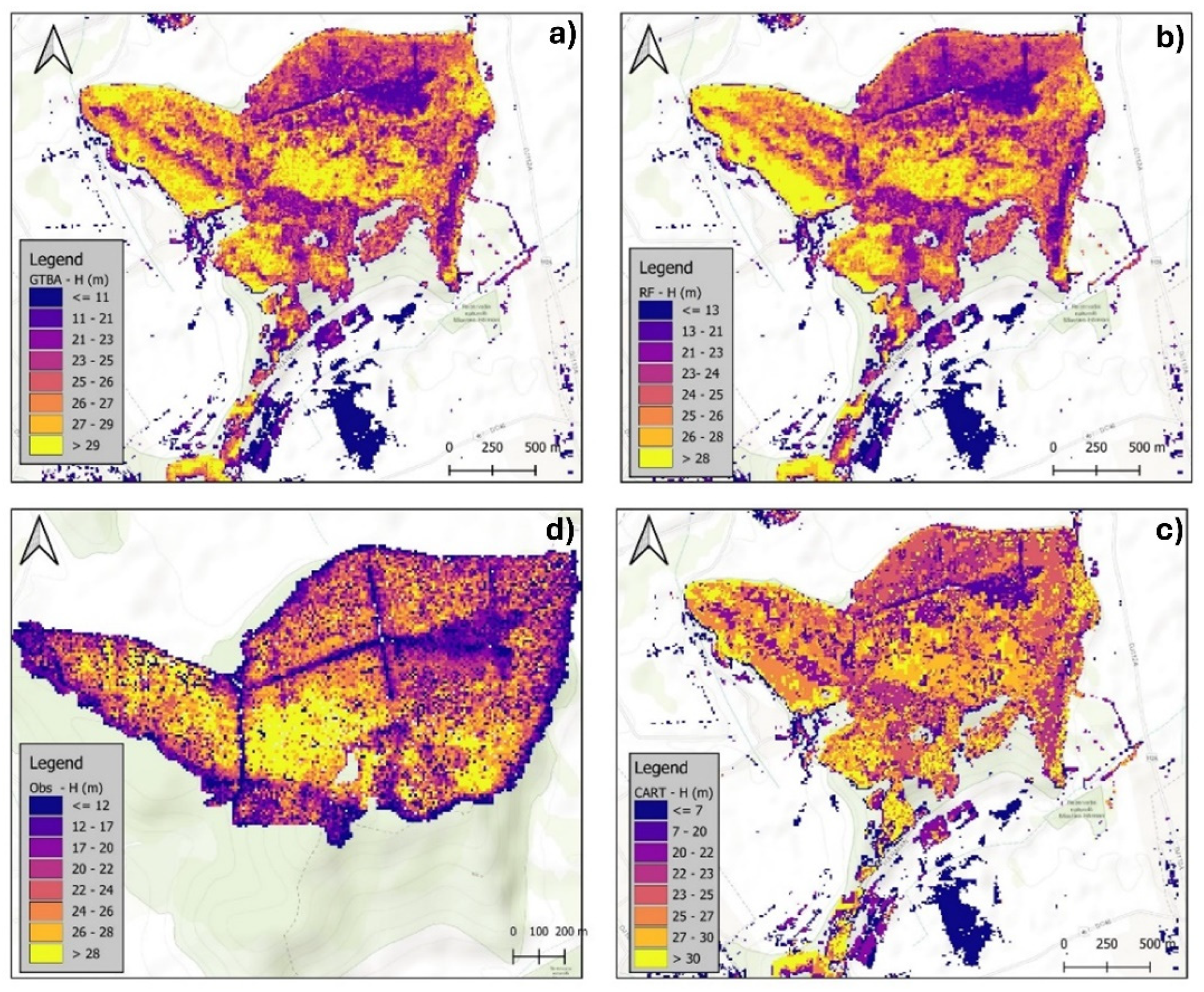
Figure 9.
Forest Characteristic Mapping for the H using: (a) CART (b) RF (c) GTBA d) Field measurements.
Figure 9.
Forest Characteristic Mapping for the H using: (a) CART (b) RF (c) GTBA d) Field measurements.
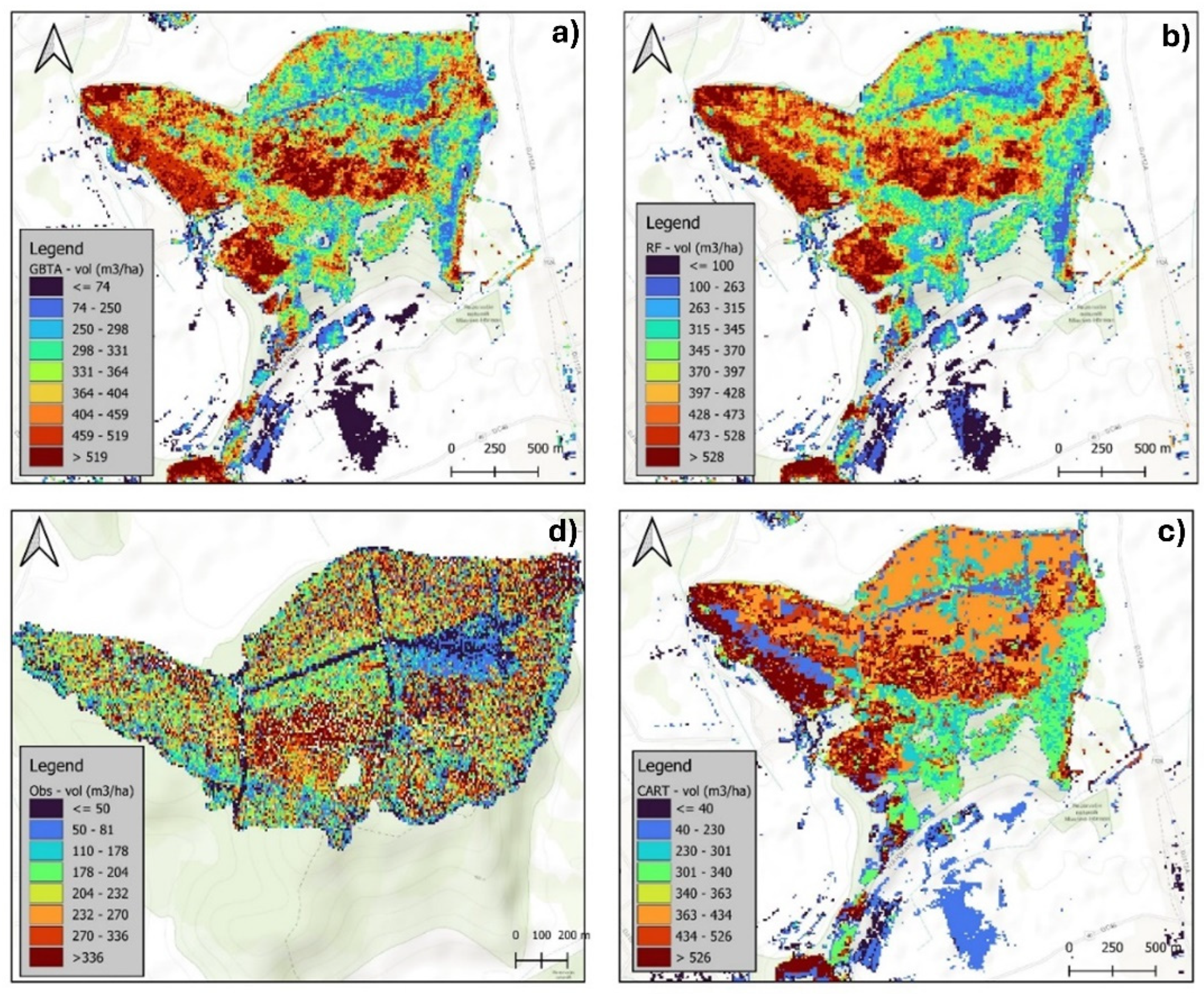
Figure 10.
Forest Characteristic Mapping for the DBH using: (a) CART (b) RF (c) GTBA d) Field measurements.
Figure 10.
Forest Characteristic Mapping for the DBH using: (a) CART (b) RF (c) GTBA d) Field measurements.
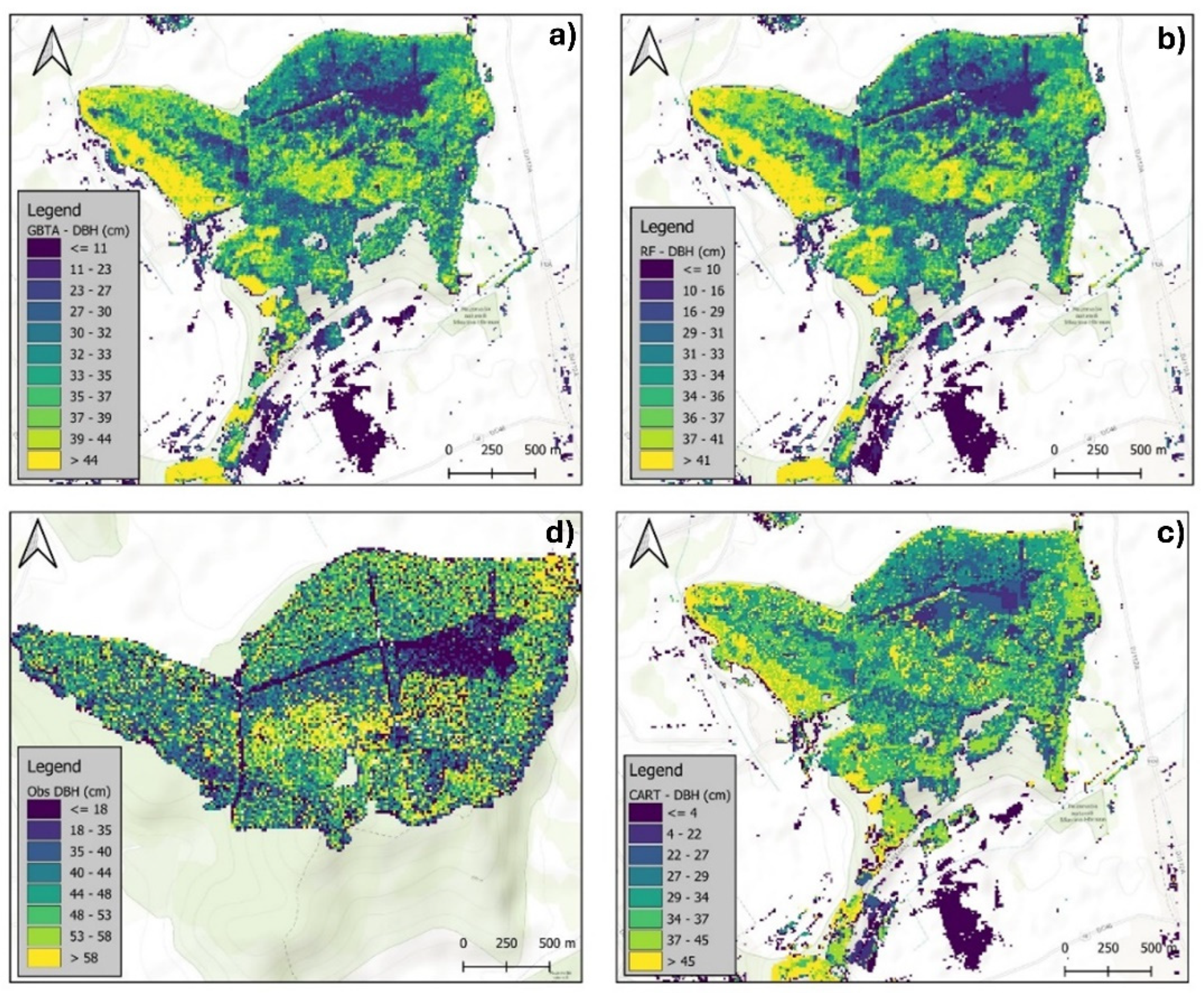
Table 3.
Performance of forest attributes estimation models with independent datasets at different resolution.
Table 3.
Performance of forest attributes estimation models with independent datasets at different resolution.
| Attribute | Algorithm | Resolution | R2 | RMSE | rRMSE(%) | MAE |
|
DBH (cm) |
RF | 10 | 0.285 | 9.200 | 0.288 | 7.921 |
| 50 | 0.297 | 6.935 | 0.212 | 6.241 | ||
| 100 | 0.578 | 5.248 | 0.162 | 4.483 | ||
| GBTA | 10 | 0.278 | 9.218 | 0.293 | 7.885 | |
| 50 | 0.312 | 6.037 | 0.186 | 7.377 | ||
| 100 | 0.596 | 4.219 | 0.138 | 4.326 | ||
| CART | 10 | 0.244 | 9.179 | 0.306 | 7.754 | |
| 50 | 0.220 | 8.974 | 0.310 | 4.752 | ||
| 100 | 0.577 | 4.982 | 0.155 | 3.498 | ||
| H | RF | 10 | 0.207 | 6.062 | 0.245 | 5.254 |
| 50 | 0.419 | 3.359 | 0.135 | 2.910 | ||
| 100 | 0.504 | 4.300 | 0.173 | 3.865 | ||
| GBTA | 10 | 0.201 | 6.091 | 0.242 | 5.418 | |
| 50 | 0.466 | 3.299 | 0.131 | 3.028 | ||
| 100 | 0.555 | 4.155 | 0.165 | 4.103 | ||
| CART | 10 | 0.176 | 6.270 | 0.260 | 5.192 | |
| 50 | 0.349 | 3.484 | 0.135 | 2.837 | ||
| 100 | 0.417 | 4.507 | 0.175 | 3.723 | ||
| Vol | RF | 10 | 0.234 | 120.943 | 0.297 | 102.554 |
| 50 | 0.215 | 59.666 | 0.149 | 49.566 | ||
| 100 | 0.286 | 66.809 | 0.1278 | 56.783 | ||
| GBTA | 10 | 0.222 | 134.598 | 0.344 | 100.610 | |
| 50 | 0.367 | 87.015 | 0.229 | 39.646 | ||
| 100 | 0.388 | 64.431 | 0.1531 | 44.834 | ||
| CART | 10 | 0.217 | 120.067 | 0.294 | 109.795 | |
| 50 | 0.061 | 50.781 | 0.148 | 65.647 | ||
| 100 | 0.360 | 59.374 | 0.1405 | 53.118 | ||
| BA | RF | 10 | 0.286 | 6.592 | 0.217 | 5.433 |
| 50 | 0.343 | 6.203 | 0.202 | 5.424 | ||
| 100 | 0.194 | 7.897 | 0.260 | 7.046 | ||
| GBTA | 10 | 0.281 | 9.285 | 0.323 | 5.723 | |
| 50 | 0.358 | 6.626 | 0.227 | 6.600 | ||
| 100 | 0.153 | 8.171 | 0.283 | 8.587 | ||
| CART | 10 | 0.351 | 6.993 | 0.228 | 7.484 | |
| 50 | 0.256 | 7.392 | 0.238 | 5.614 | ||
| 100 | 0.102 | 9.451 | 0.309 | 7.430 |
Disclaimer/Publisher’s Note: The statements, opinions and data contained in all publications are solely those of the individual author(s) and contributor(s) and not of MDPI and/or the editor(s). MDPI and/or the editor(s) disclaim responsibility for any injury to people or property resulting from any ideas, methods, instructions or products referred to in the content. |
© 2024 by the authors. Licensee MDPI, Basel, Switzerland. This article is an open access article distributed under the terms and conditions of the Creative Commons Attribution (CC BY) license (http://creativecommons.org/licenses/by/4.0/).
Copyright: This open access article is published under a Creative Commons CC BY 4.0 license, which permit the free download, distribution, and reuse, provided that the author and preprint are cited in any reuse.


