
Submitted:
24 January 2025
Posted:
24 January 2025
You are already at the latest version
Abstract
When collecting data from ERT2D (electrical resistivity tomography) and TDIPT2D (time domain IP tomography), different phenomena occur, whether natural or anthropogenic noise, which contaminate the data, and it can make their processing, analysis and interpretation difficult. Different techniques have been developed to eliminate or reduce these effects on the data, such as noise filtering or the development of new techniques for better data collection in the field. In the present work an iterative weighted least squares filter is employed after voltage normalization by current and a geometrical factor correction applied on strong topographic terrains. The selection of the filter basis function is recommended to be able to represent the natural behavior of the function to be filtered. Stationary or variable voltages in electrical prospecting decay with the inverse of the distance, which can be represented by an expansion in Legendre polynomials. On the other hand, uneven spacing of the electrodes leads to not using the correct geometric factor which results in an error in the calculation of the electrical anomaly. The efficiency of the proposed technique is analyzed and tested with field examples using different filters and applying the proposed correction factor or without using it. The results indicate a low RMS and L2-Norm error, whereby a better definition of the inverted resistivity image is obtained. For the TDIP case a better correspondence between the inverted images of resistivity and chargeability can be reached.
Keywords:
Smoothing Filter
; Legendre Polynomial
; ERT2D
; TDIP2D
; Processing
; Topographical effects
; Improving inversion
1. Introduction
In recent years, Electrical Resistivity Tomography 2D (ERT2D) and Time Domain Induced Polarization (TDIP2D) have been proven to be efficient methods for addressing problems in near surface geophysics. These methods have been particularly useful in applications such as soil contamination (Sogade et al., 2006), civil and geotechnical engineering, (Trogu, 2011; Santarato et al., 2011), archaeology (Tsokas et al., 2013), hydrogeophysics (Alfy et al., 2019), fracture flow paths (Slater et al. 1997) and dynamic processes such as water movement in vadose zones (Binley et al. 2002). They have also been used in steam injections (Ramirez et al., 1993), air spray (LaBrecque et al., 1999), contaminant transport (Newmark et al., 1998), and emerging areas such as agriculture (Allred B.; 2006) and forensic research (Sabrina, 2003, Jervis, et al., 2009).
Despite their widespread application, ERT2D and TDIP2D are often affected by noise, particularly in urban or contaminated areas, such as those polluted by hydrocarbons. In many cases, significant amounts of noisy data must be discarded to improve the inversion models, which can reduce resolution. Therefore, it is essential to develop new data collection techniques and efficient filters to minimize or remove random noise. It will allow the computation inversion process achieves more accurate and reliable inverted model
Noise in ERT data can lead to inaccurate inversion results or artifacts in the models (Gough and Sekii, 2002). This noise can be categorized as either systematic or random. Systematic noise includes electrode noise (LaBrecque et al., 2007; Dahlin et al., 2002), cultural or anthropogenic noise (Rossi et al., 2018), and noise introduced by low-pass filters in TDIP instruments, which affects the early-time decay measurements (Fiandaca et al., 2012). Other sources include inductive coupling (Sheriff, 2002). Although systematic noise is not the focus of this study, it is important to mention that can be mitigated though improved data acquisition procedures, such as nighttime measurements, techniques to reduce contact resistance noise, and the development of new electrode arrays for specific objectives as second potential difference measurements (Davydycheva et al., 2006, López et al., 2019).
Random noise (RN) on the other hand, is the subject of this study. Traditionally, RN in ERT surveys has been addressed using smoothing filters (Lei et al., 2014), sliding or median averages (Iris Instruments, 2024), and de-spike filters. Smoothing filters, such as least-squares filters, have been widely used with polynomial functions (Rossi et al., 2018; Baba et al., 2014; Bakkali, 2007) or other methods (Ritz et al., 1999) to reduce the effects of near-surface inhomogeneities that distort apparent resistivity pseudo sections. However, these studies do not explore alternative basis functions for the polynomials, as this work does.
Other approaches to reduce RN include filters based on direct and reciprocal measurements (Flores et al., 2012) and wavelet-based filters, applied to well-log data (Chandrasekhar and Rao, 2012), DC resistivity data (Li et al., 2013), and TDIP data (Deo and Cull, 2016).
For geophysicists working in the frequency domain, it is known that there is limited literature on filtering time domain IP2D data, due to the limited amount of discrete data available. Filtering TDIP frequency data depends on the equipment’s capabilities and the number of samples it can acquire. It also requires a regular lattice in both horizontal and vertical directions. More recently, full-waveform acquisition has been explored for noise suppression in TDIP data (Paine and Copeland, 2003; Rossi et al., 2018), which also require smoothing and low-pass filters.
The wavelets and frequency filters process have demonstrated well results; however, their application requires experience, time, and careful evaluation to decide where to cut signals.
Even though novel inversion methods have been developed, the most widely used ERT2D inversion approach remains the least squares methods. This method requires topographical corrections to reduce false anomalies. Additionally, smoothed data are needed to reduce root mean square (RMS) errors and to ensure the data converge well during modeling (L2- Norm < 1.0%). In practice, geometrical factor errors often arise due to inaccurate electrode spacing. Furthermore, irregular topography can alter anomalies, as some software transforms topography into a flat plane before inversion rather than considering inversion with terrain profile. Finally, field voltages are measured using different DC current values injected into the subsoil. Even though these voltages are normalized by their corresponding current during inversion, errors can occur because the entire dataset is not standardized under the same current.
In TDIP chargeability is generally not filtered, as it is considered a normalized parameter (Fox et al., 1980). However, during the inversion process, the inverted chargeability model is derived from the inverted conductivity model (Oldenburg and Li, 1994). Thus, any normalization correction or filtering applied to resistivity or conductivity data will inherently affect chargeability.
This study aims to improve smoothing filters for practitioners who frequently use ERT2D and TDIP, require enhanced signal clarity, and seek to save processing time. The proposed method involves three steps: voltage normalization, geometrical factors corrections, and an adaptive least-squares filter based on a fourth-degree Legendre polynomial (LSFLP) and a seven-sample window. This filter effectively removes random noise under the condition of equal sampling intervals and can be applied to resistivity and chargeability data.
The LSFLP can be applied independently, but when combined with voltage normalization and geometrical factor corrections, the resulting inversion models display better-defined anomalies without requiring increased smoothness or damping factors to reduce RMS errors and a L2-Norm below 1.0%.
Filtered and unfiltered data are presented for comparison. The performance of voltage normalization, geometrical factor corrections, and the LSFLP were tested on two different ERT2D field datasets and compared with a three-point moving average filter (MA) and least-squares polynomial filters (Savisky – Golay filter). The results highlight improvements in identifying small resistivity and chargeability anomalies.
2. Materials and Methods
2.1. Smoothing Filter
The main issue is to get a numerical filter that can be capable of eliminating or attenuating the effects of RN, without altering or modifying the true pattern of data. In this paper we designed a Least Square weighted filter with Legendre polynomial as basis function (LSFLP) to process the data and compare them with others very well-known filtering process: a three-point moving average filter (MA) and Savisky-Golay filter (PYTHON library SciPy; module scipy.signal; savgol-filter; x, window_length and polyorder same as LSFLP; it was applied 3 times iteratively). These three filtering methods were applied to each ERT2D and TDIP2D data set level by level.
Least Square Filter with Legendre Polynomial Basis Function
An iterative least squares smoothing method can be applied efficiently to smooth the original data. Such filter can be defined by a Legendre polynomial function of 4th degree, employing a window of 7 samples, and normalized between a rank [-1,1].
Where are Legendre polynomials and are polynomial coefficients.
An LSQF considers equally spaced samples and the smoothed filtered sample is computed by equation 2 as:
Where j=4,5,6⋯N-3, N is the number of data to be filtered.
However, an interpolation can be carried out to avoid losing the first and last three data with equations 3 written below:
The sum of coefficients must be equal to one.
In a traditional LSF coefficients remain constant, however, the LSFLP was designed as a Least Mean Square adaptive filter algorithm which can be summarized by two steps procedure to smooth data from ERT data, (Simon Haykin, 2002):
- Filtering process: A computing output response from a linear filter due to an input signal and generating an estimation error by comparing this output with a desire or reference signal.
- An adaptive process: Involve the automatic adjustment of the parameters of the filter in accordance with error estimation.
The coefficients are updated each Iteration to decrease error between a reference signal () which is considered as a freed signal of noise and the output signal ().
The function error of equation (5) is not all adequate for electrical prospecting, because the reference signal is free of noise, or it is a known signal. Our reference signal is the same as the input signal which in turn is also noise contaminated. The question now is how to update the coefficients, the answer is that it can be solved by treating the LSFLP as a weighted least squares filter. Thus, A better definition for the function error, when both functions are noise contaminated, can be defined in equation (6) (Lei et al., 2014):
Based on equation (6), an alternative relative error function can be estimated to better deal with the error.
A system of equations will have to be solved, where the elements of a weighting function W are given by the inverse value of equation (7), then:
Where P is a matrix 7x5 (column by row), is the transpose matrix of P, W is the weighted matrix, a is a coefficient vector and I is a unit vector. The elements of the square matrix (5x5) can be expressed by equation (9).
Where row =0, 1,2,3,4 and column k=0,1,2,34. The elements of (vector of 5x1) can be written as:
In a LSFLP each element (coefficients of Legendre Polynomial) of vector is determinate for each sample, which means that vector a is certainly a matrix (A) of rows 5 and 7 column which can be expressed as shown in equation 11.
If equation (11) is known, then we can interpolate the first three and last three data of the function being filtered, applying equation (3). We can also say that coefficient value represents a weighted value for the contribution of each sample.
2.2. Smoothing Process and Correction Factor Proposal
The smoothing process proposal consists of correcting the stationary and transient voltage by means of a correction factor that eliminates or reduces the effect caused by unequal electrode spacing and unequal injected current, such that the voltages collected in the field are only contaminated mainly by systematic and random noise. Once the voltages are corrected, they are filtered and new resistance, apparent resistivity and chargeability are calculated. The new recalculated parameters are already considered corrected and filtered.
To find out a correction factor, the electrical anomaly is defined as that determined for a homogeneous and isotropic half-space, where the electrode spacing and the injected current remain constant
Stationary Voltage Smoothing and Apparent Resistivity
LSFLP presents two valuable characteristics: (1) preserves the shape of the function and (2) maintains its pike values. However, a condition should be satisfied: data should be equally spaced to be filtered to obtain better performance of the filter. This condition is mostly difficult to satisfy for field data collected. Then, it is worthwhile to study the apparent resistivity (ρa) as an anomaly when it is expected to be a constant resistivity value for a homogeneous and isotropic semi space. Every value of ρa which diverges from a constant value means that the semi space is a heterogeneous one and different structures could be immersed in it. In Table 1 the electrical response of a homogeneous semi space is shown where spacing S among electrodes remains constant, and a fixed current of 1000 mA is applied for the collected data. In Table 1, apparent resistivity, voltage, and voltage/current (resistance) values describe a straight-line behavior. However, in Table 2 where current and spacing S does not remain constant, it implies that graphics for voltage and voltage/current depicted in Figure 1 do not show a straight-line behavior anymore.
1 A straight-line graphic for voltage (V), resistance (V/A) and apparent resistivity (
However, it is important to emphasize that the voltage measured in the field is correct and if the apparent resistivity were calculated with the real field geometric factor (FGF) for a half-space or topographic relief, it would be also correct. However, most of the time, it is not always possible to position these electrodes precisely. Therefore, it is suggested to measure the actual distances to calculate the real geometric factor (FGF).
Where AMF, BMF, ANF and BNF are distances between electrodes, obtained as a function of field coordinate positions.
On the other hand, calculate the apparent resistivity, it is customary to use a theoretical geometric factor (TGF), which is calculated by considering a constant spacing between electrodes (12.2) that leads to a wrong determination of the apparent resistivity value (Table 2, column 6), which would lead to the creation of spurious anomalies. (Oldenburg and Li, 1994; Zhou and Dahlin, 2003; Oldenborger et al., 2005; Pazzi et al., 2020)
Where AMT, BMT, ANT and BNT are distances between electrodes, obtained as a function of theoretical coordinate positions.
It would be valuable, if a correction factor is carrying out for collected voltages, such that all three parameters have a straight-line behavior, as if the medium would be a homogeneous and isotropic semi-space. It can be reached under two conditions: 1) equal spacing among electrodes and 2) if an arbitrary constant current of 1000 mA had been applied to all collected data (Table 1).
To find out a correction factor (CF), we assume that subsoil a homogeneous and isotropic half space, such that a correction factor can be found. It is important to establish that the corrected data will remain on the surface of the true terrain (topography), being rough or flat, and only the spacing between electrodes is corrected to an equal spacing, as well as the injected current is kept constant. Certainly, the steady and transient voltages, as well as the apparent resistivity and chargeability are all a function of the spatial coordinates (x, y, z) and the transient voltage is a function of time. Spatial coordinates are not written explicitly to make writing more agile and clear, except for the temporal variable.
Then, observed ρa will remain unaltered after correction. So, from definition of apparent resistivity:
The sub-indexes c and f define the corrected and observed parameters for voltage V and current I, respectively. If is the real current injected into the subsoil, TGF is the Theoretical Geometric Factor and FGF is the Field Geometric Factor.
From equations 12.1-12.3 the corrected voltage (Vc) is:
From equation (13) a correction factor (CF) is defined as:
The corrected resistance Rc will be defined as:
The corrected apparent resistivity will be unaltered and expressed as:
Applying equations (13), (14), (15) and (16) to field data from Table 2, we obtain the corrected data (columns 7, 8 and 9). However, if semi-space is a heterogeneous medium and then corrected voltage, corrected resistance and corrected apparent resistivity will show the same graphic behavior deviated from a straight-line.
Once the voltage is corrected, it is smoothed by applying the LSFLP proposed (equation (2) and (3)) to obtain the corrected and filtered Vc,f voltage, Rc,f resistance and ρa,f apparent resistivity.
Transient Voltage Smoothing and Chargeability
It is important to consider that chargeability is not a datum collected in the field. Chargeability (μ) is the relationship that exists between the transient voltage Vf (t) and the stationary voltage Vf, both parameters acquired in the field but at different moments. We will use the instantaneous chargeability as defined by Davydycheva et al. (2006) to clarify the filtering procedure on this parameter, then:
According to equation (14) where Vf has been corrected to be filtered, then Vf (t) should be corrected and a corrected chargeability μc should be defined. Vf (t) is measured in the field, however, it is not recorded; so, it can be recovered from equation (17) as:
Equation (18) is applicable if you have equipment capable of recording the IP drop curve in at least 20-time windows. In a case where only the overall chargeability is recorded, equation (18) can still apply.
The transient voltage must be corrected before any filtering process is applied, then in equation (18) Vf (stationary voltage) is substituted by its corrected value (equation (13) and (14))
Based upon former equations discussed it is possible to define.
The corrected chargeability (equation 20) is not the filtered function. The corrected transient voltage defined by equation 19 is the one that is filtered, and we obtain a filtered . The is a function of time and distance, so it should be filtered in both variables (same filter LSFLP is applied). The new chargeability corrected and filtered is recovered by equation (17) as:
However, the question arises whether equation (21) provides a valuable smoothed chargeability function of . To answer, it is important to analyze the chargeability from the point of view of the expected value for a relation of two functions contaminated by RN. As they have been recorded at different times, they are considered uncorrelated.
It is well known that:
Where E is the expected value, δf and δt are RN functions for stationary and transient voltage, respectively.
The expected value for chargeability can be analyzed as:
By Newton general binomial and carrying out the product we obtain
The expected value for chargeability can be expressed from equations 22 and 24 as:
If we now consider the ratio of expected value of Vf and Vf (t), then from equation 25:
Equation 26 is right up to a second order approximation, which means.
Then, from equations 26 it is possible to deduce that the expected value of the ratio would be equal to ratio of each expected value of Vf (t) and Vf.
Based upon former equations discussed and equation 22 is possible to define.
Where is the chargeability, Vc,f (t) is the transient voltage and Vc,f the stationary voltage, where all three functions have been corrected and smoothed. In Figure 2 a flow chart is depicted to visualize how both the correction factor (CF) and the filter (LSFLP) are applied.
3. Results
3.1. Archaeological Site of Mitla
The ruins of Mitla are the remains of an ancient Zapotec city originally called Lyobaa, the sacred city par excellence for the veneration of death, and whose apogee occurred during the Postclassic period, between 1200 and 1521 AD, when it concentrated the political and religious power of the central valleys of Oaxaca. The architectural group known as the Calvary Group belongs to Mitla’s Archaeological zone. It has a quadrangular plaza surrounded by four mounds dating back to the early stages of the Zapotec occupation of Mitla. The largest of these mounds, located to the east of the complex, is in the shape of a 9 m tall, stepped pyramid built of adobe with its main stairs facing west. In 1547, a chapel known by the locals as El Calvario (the Calvary) was built in the upper part of this pyramid (Figure 3). It is worth saying that the existence of this historic chapel has prevented archaeological explorations on this mound. Figure 3 shows El Calvario chapel and Schlumberger - Wenner 2D profile.
An ERT2D with a Schlumberger-Wenner array was carried out on The Calvario to study the conditions of the pyramid underlying the ground (Figure 4). The Schlumberger-Wenner profile was designed with an electrode spacing of 1.5 meters and 34 electrodes were displayed. Because the topography is rough, the data were corrected to a flat topography, as suggested by Fox (1980) for better performance of the inversion program employed for ERT2D data.
The Calvary field data was first inverted without the process proposed in this article. Afterwards, the field data was filtered only (no correction was applied) and inverted, finally the field data was corrected, filtered and inverted. Three smoothing filters were applied: Moving average (MA), a Savytzky-Golay (SG) (from an inner subroutine available from Python software) and finally with LSFLP introduced and discussed in the present paper.
Table 3 shows the parameters used with the commercial inversion software. It is worth mentioning that the three filters used allowed a damping factor of 10 and a smoothing factor of 1 with minor data manually removed. An outer loop of 2 iterations and an inner loop of 12 iterations were allowed for all the inversion done.
From Table 3 it can be deduced that 20 data were manually discarded from the field data (without filtering or correction applied). In the other hand, the RMS and L2-Norm errors are the lowest obtained in the inversion process (0.40% and 0.02%). For the Moving Average Filter case, 20 data were manually discarded when they were only filtered and inverted and when they were filtered, corrected and inverted only 11 data were discarded. The errors of the Moving Average inversions remain low and acceptable.
However, when the Savytzky-Golay Filter was applied to the Calvario data, 12 data were manually discarded (Filtered and Filtered Corrected), but the errors remained low and equal for both cases (RMS 2.05 % and L2-Norm 0.47 %). For the LSFLP filter case, for the data only filtered and inverted, 9 were discarded, the errors were 2.05% and 0.47%. When the data was filtered and corrected, 11 data were discarded and the errors slightly increased to 2.47% and 0.66%.
Analyzing the different inverted profiles the greatest discrepancies between them are found towards the sides of the structure Analyzing first the left side of the structure (Figure, 4.; box, 1.).; the greatest discrepancy is in the raw data profile (Figure, 4.a.).; which does not define the area well (resistivity around 40 Ohm*m yellow, c.o.l.o.r.).; where it is expected similar resistivity value to the right side (box, 5.; resistivity around 20 Ohm*m or green color) For boxes, 1.; 2 (Figure, 4.).; there is a better correlation between, M.A.; SG; LSFLP filters although less for, M.A. For SG and LSFLP filters a better correlation is shown.
The analysis of the profiles for the right flank of the structure (box 4 and 5) shows a better correlation between the filters used, but especially highlighting box 4.
The analysis of the central part of El Calvario is important because of the high probability that a hall is found at the top of the buried pyramid (centered at X=22.5 and Z=3.0 m), but so far, no excavation has been carried out at that site, due to the existence of the historic chapel of Calvary (El Calvario).
The analysis of the central part of the ERT profile with the different filters used clearly shows the existence of a possible hall. However, the raw data profile does not show the existence of such structure. The LSFLP profile shows a better definition of the existence of a hall, but so far, no excavation has been carried out at that site.
In summary, the left flank presents the noisiest data, however, the LSFLP inverted image shows a better agreement between the image with filtered data only (Figure 4f), and the filtered corrected image (Figure 4g). On the right flank, the filtered and filtered corrected images (Figure 4b to g) show a good agreement between them especially for box 4.
Finally, in the central area (box 3) the filtered and filtered corrected images (Figure 4b to g) show the existence of a structure (a possible hall), which is better defined in Figure 4g. The image of the raw data (Figure 4a) does not agree with the existence of the structure, and the possible explanation could be that the data were not corrected for a flat surface.
In order to visualize where the hall response can be detected in Figure 5 the apparent resistivity curve for a depth of 3 m is depicted. The electrical resistivity response of the hall can be visualized at X = 22.5 m.
3.2. Hydrocarbon Contaminated Site (North of Mexico City)
The area investigated is found within the Mexican Neovolcanic Belt and located towards the northern part of Mexico City, a heavily populated metropolis. This is in a place what used to be an important refinery owned by an oil Mexican company. Today, this plant has been converted into a park and a place of coexistence for the surrounding population. On the other hand, this place has also become a huge laboratory that has served soil researchers to learn about the effects of hydrocarbons in the subsoil. The usefulness of exploration methods, such as ERT-2D, has been of great help in detecting electrical anomalies that correspond to pollutant concentration points.
The zone is made up of volcanic-sedimentary materials from the Guerrero Terrain, covered by alluvium of sedimentary rocks from the Zimapán basin (Mexican Geological Service, 2002). Superficially, the site is covered by a gently sloping fill. There was no evidence of a regular distribution of sand and silts and there was information about a body of water around 3.5 m deep. The geological and pedological studies of the place showed that the study area was in chaos, where lenses of sand, silt and clay were found, many of them produced by the rise and fall of the surrounding water bodies. These strong variations at depth have caused further oil pollution.
Therefore the aim of this study is to delimit the contaminated regions through the anomalies (resistivity chargeability) produced by hydrocarbons (benzene) The hydrocarbon contaminated site (HC) data was inverted without the process proposed Then this data was corrected filtered inverted Three smoothing filters were applied:, M.A.; SG; LSFLP Results are shown in Figure 6 that there are seven dipole-dipole resistivity sections (left column) and their corresponding IP sections (right column) are presented.
Resistivity sections (left side Figure 6) show low values (5 Ohm*m in color blue) around 3 m depth and between boxes 2 and 3. These anomalies are correlated with the body of water described above. Also, all resistivity sections exhibit anomalies with approximately same patterns. Something different happens with IP anomalies (right side Figure 6). In this case, Figure 6b,f (box 2) do not exhibit low IP responses (-31 mV/V, blue color) as the rest of them (Figure 6dh–n). Another situation occurs in the zone within box 4, Figure 6b,f show green IP response (around 2 mV/V) and the others high IP values (35 mV/V for Figure 6d,h–n). It is also interesting that anomalies lie between boxes 2 and 3 (Figure 6d,f,h,j,l,n), where high red IP values draw different patterns. However, these anomalies are coincident between 6h (SG filtered) with 6l (LSFLP), and 6j (SG filtered and corrected) with 6n (LSFLP filtered and corrected).
Additional information is presented in Table 4 and Table 5. Table 4 shows the data of benzene concentrations in soil and water obtained in some points of the studied area. At the time of data acquisition, there was a PVC pipe installed in a well (MF21) located at position x=50.7 m (Figure 6). Furthermore, it is important to mention that the half-left zone had been almost remediate before geoelectrical data were obtained.
Table 5 shows that each section was performed by same initial data (189) Smoothing inversion damping factors were set to 10 for all sections In general this table presents a the discarded data ranged from a minimum of 13 (MA filtered) to a maximum of 25 (LSFLP) The RMS error values varied between 478 (MA filtered corrected) to 1517 (SG filtered) for resistivity 683 (MA filtered corrected) to 3787 (raw data inversion) for, I.P. The L2-Norm ranged from a minimum of 0.25 (for raw data inversion) to a maximum of 2.53 (for MA data filtered and corrected). Additionally, it shows that five sections exhibited IP RMS values approximately twice those of the RMS resistivity values (raw data inversions, MA filtered, MA filtered and corrected, SG filtered, and SG filtered and corrected). Two sections, however, showed low RMS values for both resistivity and IP within the same range. These correspond to the sections with the fewest discarded data points: MA filtered and corrected data (with RMS values of 4.78 and 6.83, and 13 discarded data points) and LSFLP data filtered and corrected (with RMS values of 10.84 and 10.29, and 15 discarded data points). Notably, MA filtered and corrected data had the highest L2-Norm (2.53), while LSFLP filtered and corrected section showed a significantly lower L2-Norm (0.72).
The half-left side of all IP figures (between boxes 1 and 2) medium values of IP persist (green color, around 2 mV/V). This behavior is explained by the remediation process mentioned earlier.
Analyzing box 3 with soil sample data from Table, 4.; reveals strong red anomalies (70 Ohm*m) correlated with high benzene concentrations (up to 86055 mg/kg for, M.F.2.1.; 50723 mg/kg for A11) This is particularly evident in Figure 6k–l (LSFLP, f.i.l.t.e.r.e.d.).; Figure 6m,n (LSFLP filtered, c.o.r.r.e.c.t.e.d.).; where high values are observed for both resistivity, I.P. A closer examinations of section 6n shows a well-defined vertical anomaly structure in box 3, around soil samples, approximately 1.5 m in diameter and extending almost the entire depth of the section. This structure corresponds to the PVC pipe mentioned above.
In box 4, Figure 6b (raw IP data inversion) and 6f (MA filtered and corrected), IP responses show medium values (around 2 mV/V). This geoelectrical response says that no contamination exists in this zone. However, the rest of IP sections (Figure 6d,h,j,l,n) depicts the opposite: high IP values (35 mV/V, red color). Also, the anomaly box 4 presents different shapes and length. Nevertheless, SG filtered (Figure 6h) seems the same as LSFLP filtered (Figure 6l), as well as SG filtered and corrected (Figure 6j) with LSFLP filtered and corrected (Figure 6n).
In summary, based on Figure 6 and Table 4 and Table 5, sections (m) and (n) demonstrate that the LSFLP (filtered and corrected) approach is both mathematically and qualitative as the best option. First, drill number MF21 (box 3) and A11 exhibit high benzene concentrations with increasing depth (Table 4). For MF21 exhibits a decreasing benzene concentration at the bottom (265.85 mg/kg at 7.2 m depth). These two drills correlate well with resistivity (Figure 6m) and IP (Figure 6n) responses. Second, these two sections achieve good L2-Norm value, minimal data loss and consistent RMS values between resistivity and IP responses.
4. Discussion
El Calvario (The Calvary), Mitla Archaeological Zone
The analysis of the errors obtained from the ERT2D images of the archaeological site of El Calvario (Table 3) shows that both the RMS and the L2-norm are low. From the analysis of the RMS and L2-norm errors alone, any of the 7 inverted images (Figure 4) would be acceptable, however there are differences between them depending on the filter applied and whether the correction factor was applied or not.
The central area is the one we will discuss, since there we can analyze the contribution of the proposal to apply a smoothing filter and the correction factor. It is important to say that the subsoil of El Calvary had not been subject to any archaeological exploration until now, so if only the raw data section had been interpreted (Figure 4a), the possible existence of the hall would have gone unnoticed. The filtered and corrected filtered ERT2D (Figure 4 b-g) from Moving Average (MA), Savitsky-Golay (SG) and Least Square Legendre Filter (LSFPL) show the existence of a rectangular structure. MA shows a well-defined and isolated hall (Figure 4 b - c), while SG shows a slightly longer hall (Figure 4 d - e).
Finally, the inverted ERT2D from LSFLP shows a well-defined hall (Figure 4 f- g), especially the one in Figure 4g. In summary, the ERT2D study of The Calvary shows the valuable contribution of applying a smoothed filtering and correction factor for ERT2D data collected in difficult terrain to improve inversion models.
Hydrocarbon Contaminated Site (North of Mexico City)
In the case of the hydrocarbon-contaminated site, differences were observed between filtered and filtered and corrected datasets. For instance, in the resistivity data (left column of Figure 6) at the bottom of box 3, the filtered and corrected for MA (Figure 6e) and for LSFLP (Figure 6m) show strong and defined anomalies with high resistivity values (red color). These anomalies correlate with high benzene concentrations. In contrast, these red anomalies do not appear in the filtered data (Figure 6c) and the SG sections (Figure 6g,i).
5. Conclusions
Certainly, any filtering process applied to a data set influences the interpretation of the electrical anomalies. Therefore, it is recommended that the filter and any other process be used to improve the data alter as little as possible the original shape of the ERT and TDIPT anomalies.
The introduced process of employing a smoothing filter and a correction factor seeks to satisfy as much as possible what is expressed in the previous paragraph. From the examples discussed, resistivity data from electrical resistive tomography is less affected by the smoothing filter used, however, the proposed LSFLP filter in the present paper showed a better performance, as deduced from the 2D electrical resistivity tomography of the archaeological zone of Mitla.
To filter the resistivity data with the proposed process, it is recommended to use a maximum of 3 iterations and apply the correction factor (CF), as well as collect the field data level by level.
On the other hand, the chargeability anomaly is more affected by the treatment applied, as shown in the case of soil contamination by hydrocarbons. For the chargeability of the raw data, a clear correlation between resistivity anomaly and chargeability is not defined, as would be expected.
For the moving average filter, there is a better result in anomalies shape and differences are observed between the filtered data (Figure 6.d) and filtered and corrected (Figure 6.f), but a better correlation between resistivity and chargeability can be established.
For the Savitzky-Golay filter, a better image of the inverted chargeability is obtained, although there is somewhat different between filtered data (Figure 6h) and those filtered corrected (Figure 6j).
A final observation, in the ERT and TDIPT, no correction was made for electrode position; however, the correction to a constant current was applied.
As a note, MA and Savitzky - Golay filters were used as feedback filters. The correction for electrode positioning was not possible to apply, however, the correction for a constant current of 1000 mA was applied.
Finally, for LSFLP inverted chargeability images show a better correlation with resistivity, but there are differences between the filtered data (Figure 6.l) and those filtered corrected (6.n). The LSFLP filter was designed as an iterative filter, and 3 iteration were allowed.
References
- Alfy, M.E.; Lashin, A.; Faraj, T.; Alataway, A.; Tarawneh, Q.; Al-Bassam, A. Quantitative hydro-geophysical analysis of a complex structural karst aquifer in Eastern Saudi Arabia. Scientific Reports 2019, 9, 2825. [Google Scholar] [CrossRef] [PubMed]
- Allred, B.; Reza, E.M.; Saraswat, D. Comparison of electromagnetic induction, capacitively-coupled resistivity, and galvanic contact resistivity methods for soil electrical conductivity measurement. Applied Engineering in Agriculture, 2006, 22, 215–230. [Google Scholar] [CrossRef]
- Baba, K.; Bahi, L.; Ouadif, L. Enhancing geophysical signals through the use of Savitzky-Golay filtering method. Geofísica Internacional, 2014, 53, 399–409. Available online: https://www.scielo.org.mx/scielo.php?script=sci_arttext&pid=S0016-71692014000400003&lng=es&tlng=en (accessed on 21 April 2022). [CrossRef]
- Bakkali, S. Using Savitzky-Golay filtering method to optimize surface phosphate deposit disturbances. Ingenierías, 2007, 10, 35. [Google Scholar]
- Binley, A.; Cassiani, G.; Middleton, R.; Winship, P. Vadose zone flow model parameterization using cross-borehole radar and resistivity imaging. Journal od Hydrology, 2002, 267, 147–159. [Google Scholar] [CrossRef]
- Chandrasekhar, E.; Eswara Rao, V. Wavelet Analysis of Geophysical Well-log Data of Bombay Offshore Basin, India. Mathematical Geosciences, 2012, 44, 901–928. [Google Scholar] [CrossRef]
- Dahlin, T.; Leroux, V.; Nissen, J. Measuring techniques in induced polarization imaging. Journal of Applied Geophysics, 2002, 50, 279–298. [Google Scholar] [CrossRef]
- Davydycheva, S.; Rykhlinski, N.; Legeido, P. Electrical-prospecting method for hydrocarbon search using the induced-polarization effect. Geophysics, 2006, 71, G179–189. [Google Scholar] [CrossRef]
- Deo, R.N.; Cull, J.P. Denoising time-domain induced polarization data using wavelet techniques. Exploration Geophysics, 2016, 47, 108–114. [Google Scholar] [CrossRef]
- Ferrari, L.; Orozco-Esquivel, T.; Navarro, M.; López-Quiroz, P.; Luna, L. Digital Geologic Cartography and Geochronologic Database of the Trans-Mexican Volcanic Belt and Adjoining Area. Terra Digitalis, 2018, 3, 1. [Google Scholar] [CrossRef]
- Ferrari, L.; Tagami, T.; Eguchi, M.; Orozco-Esquivel, M.T.; Petrone, C.M.; Jacobo Albarrán, J.; LópezMartínez, M. Geology, geochronology and tectonic setting of late Cenozoic volcanism along the south-western Gulf of Mexico: The Eastern Alkaline Province revisited. Journal of Volcanology and Geothermal Research 2005, 146, 284–306. [Google Scholar] [CrossRef]
- Fiandaca, G.; Auken, E.; Christiansen, A.V.; Gazoty, A. Time domain induced polarization: full-decay forward modelling and 1D laterally constrained inversion of Cole-Cole parameters. GEOPHYSICS, 2012, 77, E213–E225. [Google Scholar] [CrossRef]
- Flores, A.; Kemna, A.; Zimmermann, E. Data error quantification in spectral induced polarization imaging. GEOPHYSICS, 2012, 77, E227–E237. [Google Scholar]
- Fox, R.C.; Hohmann, G.W.; Killpack, T.J.; y Rijo, L. Topographyc effects in resistivity and induced polarization surveys. Geophysics, 1980, 45, 75–93. [Google Scholar] [CrossRef]
- Gough, D.O.; Sekii, T. On the effect of error correlation on linear inversions. Monthly Notices of the Royal Astronomical Society, 2002, 335, 170–176. [Google Scholar] [CrossRef]
- Haykin, S.; Adaptive Filter Theory, 4th ed. Upper Saddle River, NJ: Prentice-Hall, 2002.
- Iris Instruments. Processing software. Available online: https://www.iris-instruments.com/syscal-prosw.html (accessed on 11 May 2024).
- Jervis, R.; Pringle, J.K.; Tuckwell, G.W. Time-lapse resistivity surveys over simulated clandestine graves. Forensic Science International, 2009, 192, 7–13. [Google Scholar] [CrossRef]
- LaBrecque, D.J.; Morelli, G.; Daily, W.; Ramirez, A.; Lundegard, P.; 1999, Occam’s inversion of 3-D electrical resistivity tomography. Three-Dimensional Electromagnetics. January 1999, 575-590.
- LaBrecque, D.; Daily, W.; Adkins, P. Systematic errors in resistivity measurement systems: Presented at the 20th EEGS Symposium on the Application of Geophysics to Engineering and Environmental Problems, European Association of Geoscientists & Engineers. 2007. [CrossRef]
- Lei, Z.; Tianqi, G.; Ji, Z.; Shijun, J.; Qingzhou, S.; Ming, H. An adaptive moving least squares method for curve fitting. Measurement 2014, 49, 107–112. [Google Scholar] [CrossRef]
- Li, J.; Zhanxiang, H.; Liu, Q.H. Higher-order statistics correlation stacking for DC electrical data in the wavelet domain. Journal of Applied Geophysics, 2013, 99, 51–59. [Google Scholar] [CrossRef]
- López-González, A.E.; Tejero-Andrade, A.; Hernández-Martínez, J.L.; Prado, B.; Chávez, R.E. Induced Polarization and Resistivity of Second Potential Differences (SDP) with Focused Sources Applied to Environmental Problems. Journal of Environmental and Engineering Geophysics, 2019, 24, 49–61. [Google Scholar] [CrossRef]
- Mexican Geological Service, 2002, Carta Geológico-Minera Ciudad de México E14-2, Estado de México, Tlaxcala, Distrito Federal, Puebla, Hidalgo y Morelos., escala 1:250000: Pachuca, Hidalgo., Primera Edición.
- Newmark, R.; Aines, R.; Hudson, G.; Lif, R.; Chiarappa, M.; Carrigan, C.; Nitao, J.; Elsholz, A.; Eaker, C. An integrated approach to monitoring a field test of in situ contaminant destruction. Symposium on the Application of Geophysics to Engineering and Environmental Problems. 1999, 527–539. [Google Scholar] [CrossRef]
- Oldenburg, D.; Li, Y. Inversion of induced polarization data. Geophysics 1994, 59, 1327–1341. [Google Scholar] [CrossRef]
- Paine, J.; Copeland, A. Reduction of noise in induced polarization data using full time-series data. Exploration Geophysics, 2003, 34, 225–228. [Google Scholar] [CrossRef]
- Ramirez, A.; Daily, W.; LaBrecque, D.; Owen, E.; Chestnut, D. Monitoring an underground steam injection process using electrical resistance tomography, Water Resource. Res., 1993, 29, 73–87. [Google Scholar]
- Ritz, M.; Robain, H.; Pervago, E.; Albouy, Y. ; Camerlynck. C.; Descloitres, M.; Mariko, A. Improvement to resistivity pseudosection modelling by removal of near-surface inhomogeneity effects: application to a soil system in south Cameroon. Geophysical Prospecting, 1999, 47, 85–101. [Google Scholar]
- Rossi, M.; Dahlin, T.; Olsson, P.-I.; Günther, T. Data acquisition, processing and filtering for reliable 3D resistivity and time-domain induced polarization tomography in an urban area: field example of Vinsta, Stockholm. Near Surface Geophysics, 2018, 16, 220–229. [Google Scholar] [CrossRef]
- Sabrina, B. Searching for graves using geophysical technology: field Tests with ground penetrating radar, magnetometry, and electrical resistivity. Journal of Forensic Science, 2003, 48, 5–11. [Google Scholar]
- Santarato, G.; Ranieri, G.; Occhi, M.; Morelli, G.; Fischanger, F.; Gualerzi, D. Three-dimensional Electrical Resistivity Tomography to control the injection of expanding resins for the treatment and stabilization of foundation soils: Engineering Geology, 119, Issues 1-2, 18-30. Three-dimensional electrical resistivity tomography to control the injection of expanding resins for the treatment and stabilization of foundation soils. Engineering Geology, 2011, 119, 18–30. [Google Scholar]
- Savitzky, A.; Golay, M.J.E. Smoothing and differentiations of data by simplified least squares procedures. Analytical chemistry, 1964, 36, 1627–1639. [Google Scholar] [CrossRef]
- Sheriff, R.E. Encyclopedic Dictionary of Applied Geophysics: Society of Exploration Geophysicist, Fourth Edition. 2002. ISBN: 978-1-56080-118-4.
- . [CrossRef]
- Slater, L.; Binley, A.; Brown, D. Electrical Imaging of Fractures Using Ground-Water Salinity Change. Ground Water, 1997, 35, 436–442. [Google Scholar] [CrossRef]
- Sogade, J.A.; Scira-Scarppuzzo, F.; Vichabian, Y.; Shi, W.; Rodi, W.; Lesmes, D.P.; Morgan, F.D. Induced-polarization and mapping of contaminant plumes. GEOPHYSICS, 2006, 71, B75–B84. [Google Scholar] [CrossRef]
- Trogu, A.; Rainiere, G.; and Fischanger, F. 3D Electrical Resistivity Tomography to Improve the Knowledge of the subsoil below Existing Buildings. Environmental Semeiotics, 2011, 4, 63–70. [Google Scholar] [CrossRef]
- Tsokas, G.N.; Diamanti, N.; Tsourlos, P.I.; Vargemezis, G.; Stampolidis, A.; Raptis, K.T. Geophysical prospection at Hamza bey (Alkazar) monument, Thessaloniki, Greece. Mediterranean Archaeology Archaeometry, 2013, 13, 9e20. [Google Scholar]
Figure 1.
Observed voltage and resistance when current and electrodes spacing do not remain constant. A smoothed voltage is recovered when has been corrected.
Figure 1.
Observed voltage and resistance when current and electrodes spacing do not remain constant. A smoothed voltage is recovered when has been corrected.
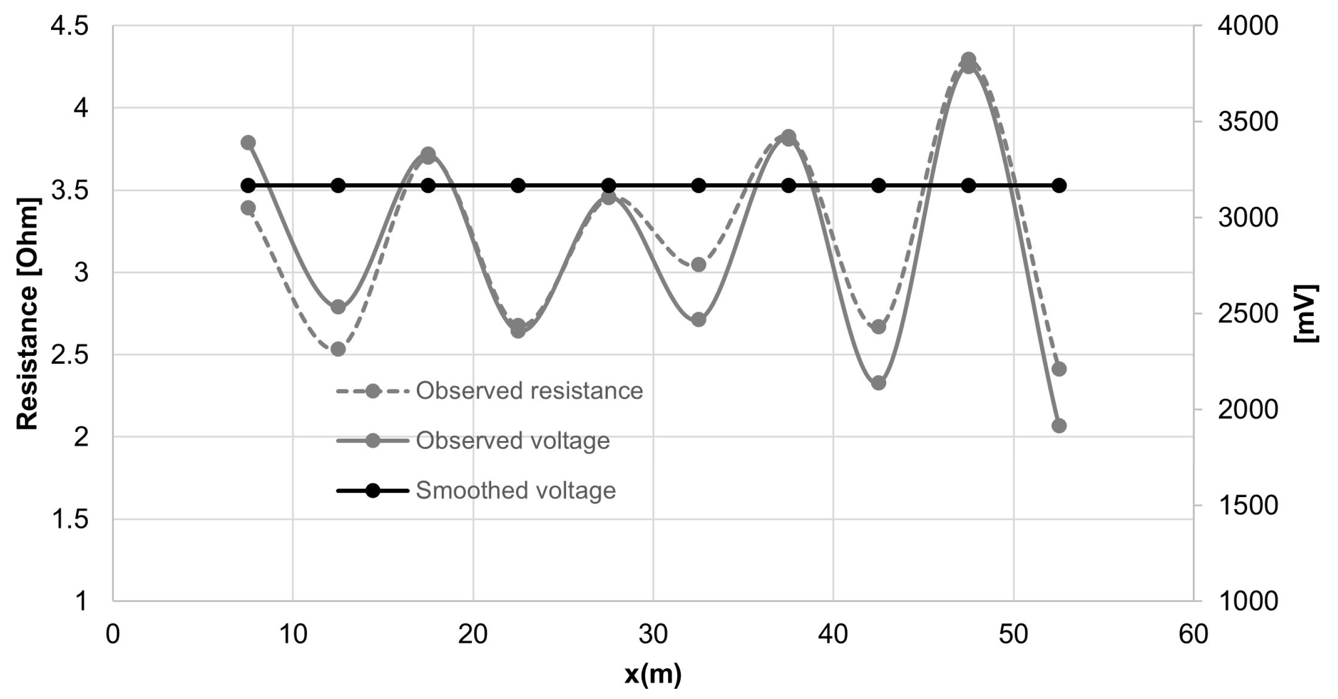
Figure 2.
Flow chart of the method proposal.
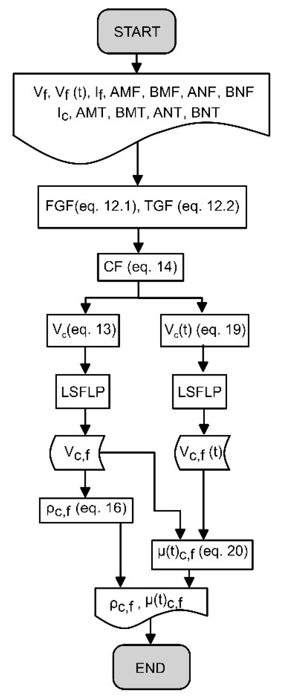
Figure 3.
El Calvario (The Calvary) and the Schlumberger – Wenner 2D profile.
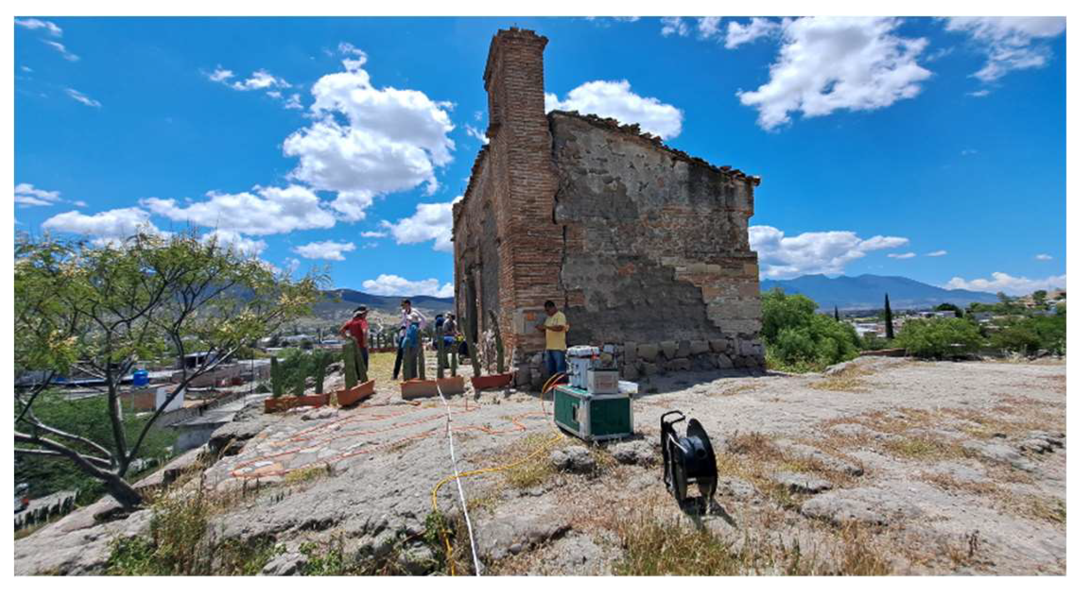
Figure 4.
The Calvary, ERT2D images. Seven resistivity sections were obtained from next data: (a) Raw resistivity data; (b) MA filtered data; (c) MA filtered and corrected data; (d) SG filtered data; (e) SG filtered and corrected data; (f) LSQFLP filtered data; (g) LSQFLP filtered and corrected data.
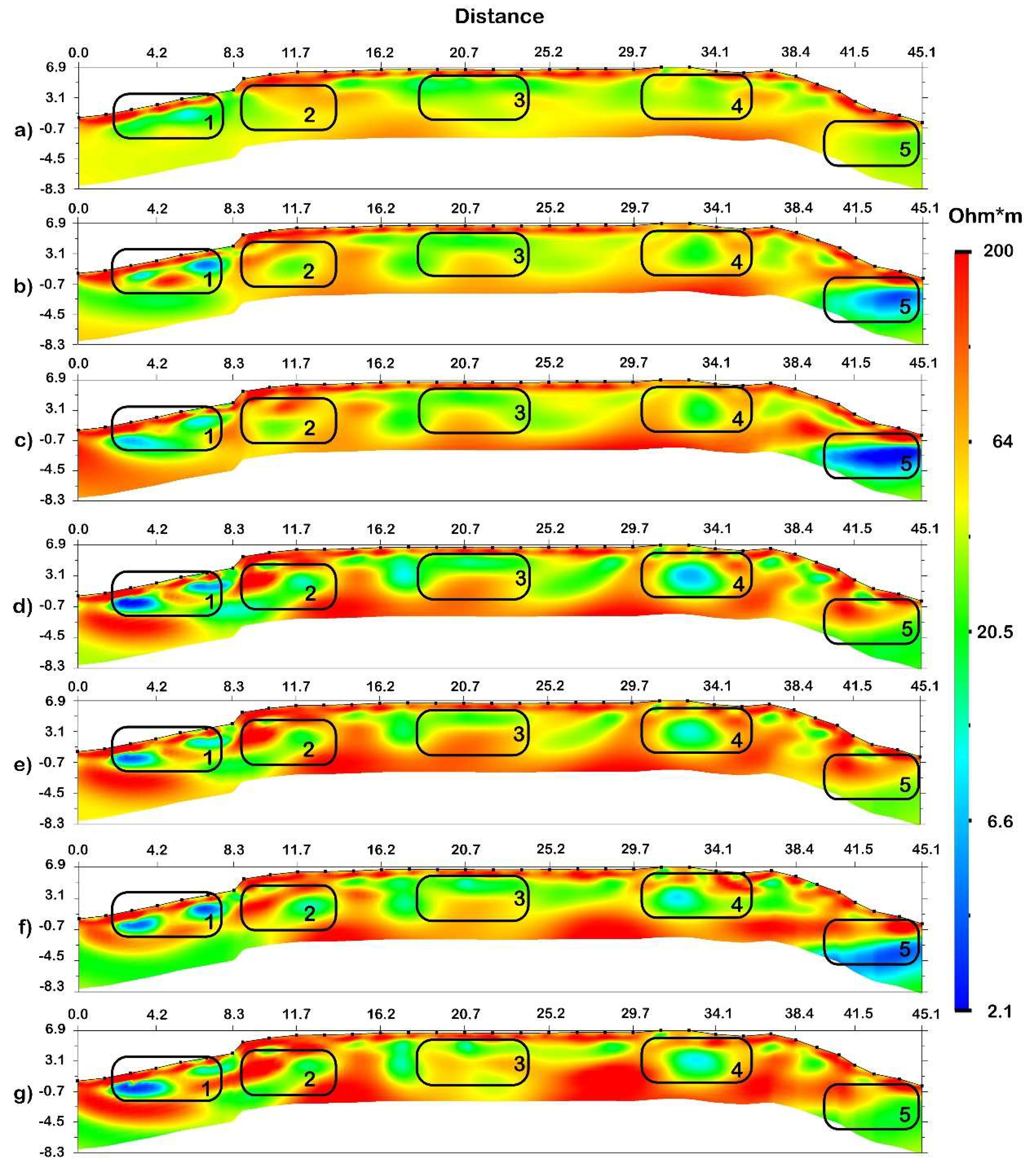
Figure 5.
The apparent resistivity curves for the Calvary site at a depth of 3 m are presented. The hall response is at X = 22.5 m. Raw (original data), moving average (MA), Savytzky-Golay (SG) and a least square weighted filter with Legendre polynomial (LSFLP).
Figure 5.
The apparent resistivity curves for the Calvary site at a depth of 3 m are presented. The hall response is at X = 22.5 m. Raw (original data), moving average (MA), Savytzky-Golay (SG) and a least square weighted filter with Legendre polynomial (LSFLP).
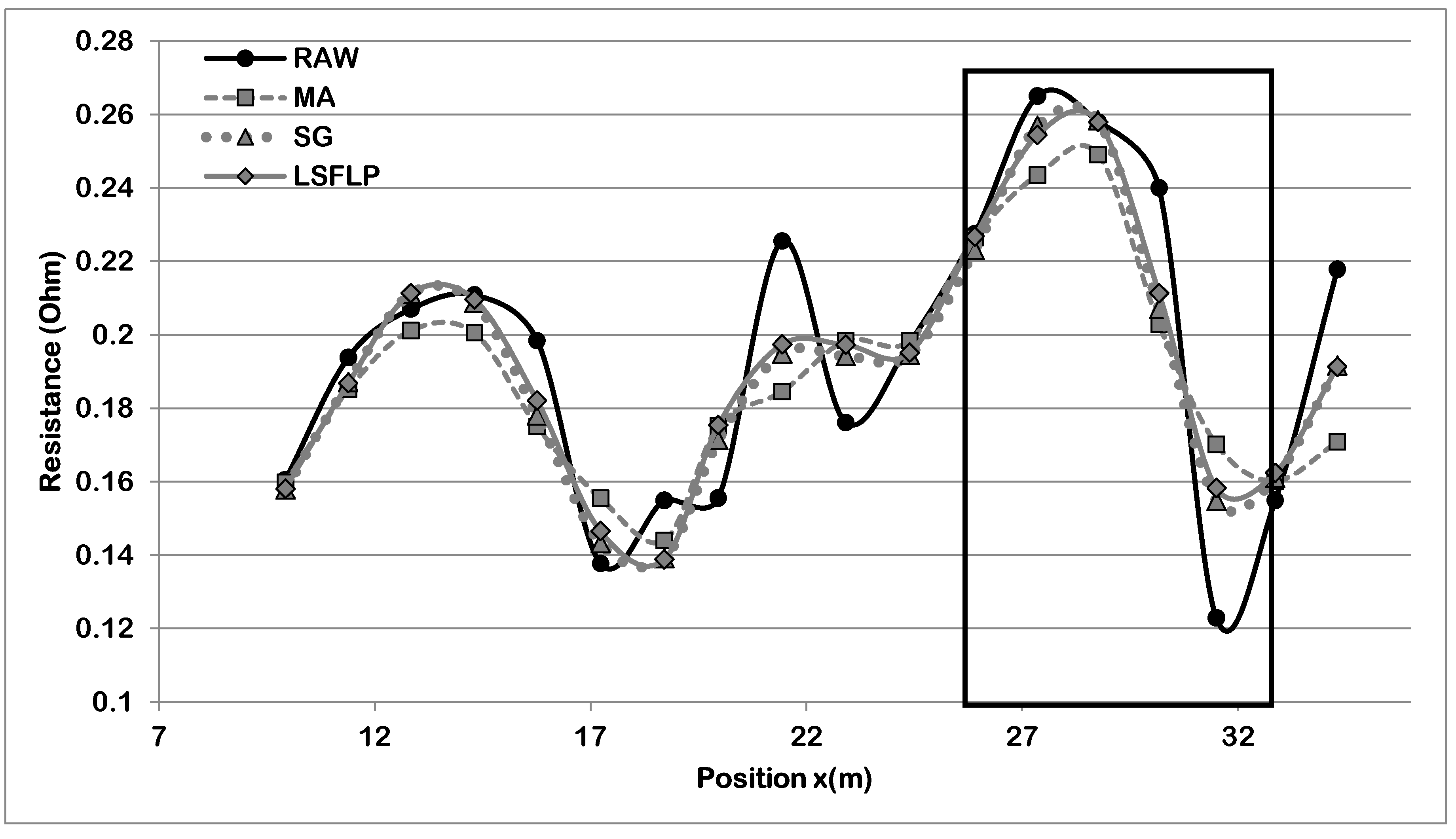
Figure 6.
Hydrocarbon contaminated sections ERT2D. Seven resistivity sections were obtained : Raw resistivity section and (a) its IP section (b) ; (c) MA filtered resistivity data section and (d) its IP section ; (e) MA filtered and corrected data and (f) its IP section ; (g) SG filtered data and (h) its IP section ; (i) SG filtered and corrected data and (j) its IP section ; (k) LSQFLP filtered data and (l) its IP section ; (m) LSQFLP filtered and corrected data and (n) its IP section. Drill’s name 21, 25, MF21 and A11 are shown at the top of the figure on each column. Red represents high values. Blue represents low values.

Table 1.
Values from a constant depth in a homogeneous half-space.
| x(m) | FGF | Current (A) | Voltage (V) | (V/A) | |
|---|---|---|---|---|---|
| 7.54 | 31.57 | 1000 | 3167.56 | 3.17 | 100 |
| 12.56 | 31.57 | 1000 | 3167.56 | 3.17 | 100 |
| 17.58 | 31.57 | 1000 | 3167.56 | 3.17 | 100 |
| 22.61 | 31.57 | 1000 | 3167.56 | 3.17 | 100 |
| 27.63 | 31.57 | 1000 | 3167.56 | 3.17 | 100 |
| 32.66 | 31.57 | 1000 | 3167.56 | 3.17 | 100 |
| 37.68 | 31.57 | 1000 | 3167.56 | 3.17 | 100 |
| 42.70 | 31.57 | 1000 | 3167.56 | 3.17 | 100 |
| 47.73 | 31.57 | 1000 | 3167.56 | 3.17 | 100 |
| 52.75 | 31.57 | 1000 | 3167.56 | 3.17 | 100 |
)is obtained from a horizontal linear (x(m)) at 2.6 m depth, homogeneous, and isotropic half-space medium. Current (A) is constant and spacing between electrodes is equal for all data.
Table 2.
Field and corrected data comparison from a non-equal spaced data acquisition.
| Geometric factor | Field data | Corrected data | ||||||
|---|---|---|---|---|---|---|---|---|
| Field | Teoretical | (A) | (V) | (V/A) | V | (V/A) | ||
| 29.49 | 31.57 | 1000 | 3390.979 | 3.390979 | 107.0532 | 3167.56414 | 3.167564 | 100 |
| 39.46 | 31.57 | 1000 | 2534.211 | 2.534211 | 80.00506 | 3167.56414 | 3.167564 | 100 |
| 27.03 | 31.57 | 900 | 3329.633 | 3.699593 | 116.7961 | 3167.56414 | 3.167564 | 100 |
| 37.36 | 31.57 | 900 | 2408.993 | 2.676659 | 84.50214 | 3167.56414 | 3.167564 | 100 |
| 28.95 | 31.57 | 900 | 3108.808 | 3.454231 | 109.0500 | 3167.56414 | 3.167564 | 100 |
| 32.82 | 31.57 | 810 | 2468.007 | 3.046922 | 96.19134 | 3167.56414 | 3.167564 | 100 |
| 26.13 | 31.57 | 891 | 3409.873 | 3.827018 | 120.8189 | 3167.56414 | 3.167564 | 100 |
| 37.47 | 31.57 | 801.9 | 2140.112 | 2.668801 | 84.25406 | 3167.56414 | 3.167564 | 100 |
| 23.29 | 31.57 | 882.09 | 3787.419 | 4.293688 | 135.5517 | 3167.56414 | 3.167564 | 100 |
| 41.43 | 31.57 | 793.881 | 1916.198 | 2.413709 | 76.20082 | 3167.56414 | 3.167564 | 100 |
* Columns 4, 5 and 6 depict behavior when the condition of Table 1 is not satisfied. Columns 7,8 and 9 when a corrected factor CF (equation 14) is applied.
Table 3.
Inversion data information from each section on Figure 4.
Table 3.
Inversion data information from each section on Figure 4.
| Initial data |
Final data |
Discarded data | RMS % | L2-Norm | Damping factor |
Smoothing factor |
|
|---|---|---|---|---|---|---|---|
| Raw data | 247 | 227 | 20 | 0.40 | 0.02 | 10.0 | 1.0 |
| MA Filtered | 247 | 227 | 20 | 0.97 | 0.10 | 10.0 | 1.0 |
| MA Filtered and Corrected | 247 | 236 | 11 | 0.98 | 0.11 | 10.0 | 1.0 |
| SG Filtered | 247 | 235 | 12 | 2.05 | 0.47 | 10.0 | 1.0 |
| SG Filtered and Corrected | 247 | 235 | 12 | 2.05 | 0.47 | 10.0 | 1.0 |
| LSQFLP Filtered | 247 | 238 | 9 | 2.05 | 0.47 | 10.0 | 1.0 |
| LSQFLP Filtered and Corrected | 247 | 236 | 11 | 2.43 | 0.66 | 10.0 | 1.0 |
Table 4.
Inversion data information from each section on Figure 5.
Table 4.
Inversion data information from each section on Figure 5.
|
Depth (m) |
21 (mg/L) |
25 (mg/L) |
MF21 (mg/kg) |
A11 (mg/kg) |
| 1.2 | 0.78 | 0.80 | ||
| 2.4 | 3.46 | 0.82 | ||
| 3.6 | 57.77 | 19.17 | ||
| 4.8 | 362.79 | 21.90 | ||
| 6.0 | 860.55 | 157.06 | ||
| 7.2 | 40.891 | 399.753 | 265.85 | 507.23 |
| 8.4 | 3329.74 | 896.92 |
* Only two samples were taken in water: one for drill number 21 and the other for drill number 25
Table 5.
Inversion data information from each section on Figure 5.
Table 5.
Inversion data information from each section on Figure 5.
| Initial data |
Final data |
Discarded data | RMS % | L2-Norm | ||
|---|---|---|---|---|---|---|
| Raw data | Resistivity Chargeability |
189 | 171 | 18 | 16.27 37.87 |
0.25 |
| MA filtered | Resistivity Chargeability |
189 | 176 | 13 | 6.99 18.92 |
0.52 |
| MA filtered and corrected | Resistivity Chargeability |
189 | 168 | 21 | 4.78 6.83 |
2.53 |
| SG filtered | Resistivity Chargeability |
189 | 166 | 23 | 7.59 15.21 |
0.60 |
| SG filtered and corrected | Resistivity Chargeability |
189 | 171 | 17 | 4.74 10.74 |
0.53 |
| LSFLP filtered | Resistivity Chargeability |
189 | 164 | 25 | 10.85 14.75 |
0.57 |
| LSFLP filtered and corrected | Resistivity Chargeability |
189 | 174 | 15 | 10.84 11.32 |
0.72 |
* Discarded data is a tool within inversion software, where several data are suggested to delete to get a better RMS. This option is displayed by a histogram data option.
Disclaimer/Publisher’s Note: The statements, opinions and data contained in all publications are solely those of the individual author(s) and contributor(s) and not of MDPI and/or the editor(s). MDPI and/or the editor(s) disclaim responsibility for any injury to people or property resulting from any ideas, methods, instructions or products referred to in the content. |
© 2025 by the authors. Licensee MDPI, Basel, Switzerland. This article is an open access article distributed under the terms and conditions of the Creative Commons Attribution (CC BY) license (http://creativecommons.org/licenses/by/4.0/).
Copyright: This open access article is published under a Creative Commons CC BY 4.0 license, which permit the free download, distribution, and reuse, provided that the author and preprint are cited in any reuse.


