Submitted:
21 June 2025
Posted:
24 June 2025
You are already at the latest version
Abstract
With the increasing frequency of marine activities, the significance of underwater target search and rescue has been highlighted, where precise and efficient path planning is critical for ensuring search effectiveness. This study proposes an underwater target search path planning method by incorporating the dynamic variations of marine acoustic environments driven by sea surface wind fields. First, wind-generated noise levels are calculated based on the sea surface wind field data of the mission area, and transmission loss is solved using an underwater acoustic propagation ray model. Then, a spatially variant search distance matrix is constructed by integrating the active sonar equation. Finally, a sixteen-azimuth path planning model is established, and a genetic algorithm (GA) is introduced to optimize the search path for maximum coverage. Numerical simulations in three typical sea areas (the South China Sea, Atlantic Ocean, and Pacific Ocean) demonstrate that the optimized search coverage of the proposed method increases by 54.32%–130.22% compared with the pre-optimization results, providing an efficient and feasible solution for underwater target search.
Keywords:
Underwater target search
; Path planning
; Sea surface wind field
; Underwater acoustic environment
; Genetic algorithm
1. Introduction
With the acceleration of globalization, the density of maritime traffic has been continuously increasing. Coupled with the frequent occurrence of extreme weather events, maritime search and rescue as well as underwater target detection tasks have become increasingly complex and urgent [1]. The helicopter maritime loss-of-contact incident in Japan on April 6, 2025, and the disappearance of the "Lucky Harvest" vessel on May 13, 2025, have brought widespread attention to underwater target search.
Underwater target search is one of the key technologies for ensuring navigation safety, and precise and efficient path planning is crucial to guaranteeing search effectiveness. In recent years, scholars have proposed various path planning algorithms for underwater target search. In 2020, Yu et al. [2] applied the particle swarm optimization (PSO) algorithm to collaborative tasks of multi-unmanned platforms, including unmanned aerial vehicle (UAV), unmanned surface vehicles (USV), and autonomous underwater vehicle (AUV), achieving efficient cooperative search. In 2023, Niu et al. [3] proposed a multi-AUV collaborative search model combining the improved k-means algorithm and PSO, further optimizing search path planning by constructing target scattering models and sonar search models. Yibing Li et al. [4] proposed a Voronoi diagram-based task allocation method in 2024, which extracts high-value sub-regions through peak filtering and achieves load balancing using a consensus bundling algorithm. On this basis, path planning combined with an improved Glasius bio-inspired neural network significantly enhances search efficiency. In the same year, Zekun Bai et al. [5] proposed an improved double deep Q-networks algorithm, which further improves global search capability and convergence performance by designing a reward function integrated with heuristic functions. Experimental results show that the algorithm performs excellently in complex unknown environments, generating safer and shorter global paths. In 2025, Qian Longxia et al. [6] proposed a hidden Markov model-Dijkstra underwater target search model and designed two search deployment algorithms. This method selects grid points as deployment positions by inversely sorting concealment evaluation data and realizes path planning by combining the improved Dijkstra algorithm, significantly improving search performance and stability. Zhe Cao et al. [7] proposed a multi-AUV collaborative adaptive coverage path planning algorithm, which initially formulates navigation paths through the neuronal activity reassigned algorithm, then optimizes the path planning process using a Glasius bio-inspired neural network. Finally, task area allocation is rationalized via the adaptive balance evolution algorithm, reducing path repetition rate and turning times. Qi et al. [8,9] proposed an improved heuristic rapidly-exploring random trees algorithm based on the velocity vector synthesis method, which counteracts ocean current effects by synthesizing AUV velocity vectors with current velocity vectors, enhancing AUV anti-ocean current disturbance capability. Experimental results show that the algorithm significantly narrows the search space while balancing path safety and smoothness. However, current research on underwater target search path planning rarely considers the influence of the marine acoustic environment, and the impact of sea surface wind fields on path planning has not been mentioned.
Sea surface wind fields affect the propagation characteristics of sound waves in underwater media [10,11], thereby influencing underwater target search path planning. In the field of underwater target search, sound waves are currently the only energy carriers capable of long-distance propagation underwater, playing a core and irreplaceable role. Sonars receiving acoustic signals reflected or emitted by underwater targets serve as the primary means for underwater target recognition and localization [12], with their performance described by the sonar equation. This requires considering parameters such as source level, transmission loss, target strength, receiving array directivity index, noise level, and detection threshold [13]. Among these, the noise level is one of the key factors affecting sonar search range. The noise level is a parameter describing the intensity of marine ambient noise, which results from the combined action of multiple noise sources, such as tides and waves, marine turbulence, ship noise, wind-generated noise, and thermal noise [14]. According to the Wenz spectrum [15], when the sound wave frequency is in the range of 100 Hz to 20 kHz, wind-generated noise is the main influencing factor, and the noise level is directly related to the wind speed at the location of the hydrophone. Hildebrand et al. [16] proposed an empirical model of wind-generated noise through statistical analysis of more than 100 years of wind-generated noise, showing a smaller slope (approximately 5 dB/decade) in the lower frequency band (10–100 Hz) and an increased slope to approximately 15 dB/decade in the high-frequency band (400 Hz–20 kHz) [16,17]. Wang Yang et al. [18] constructed a numerical calculation model of deep-sea wind-generated noise by combining the Harrison wind-generated noise source level formula with a sea surface noise transmission model. Although scholars have conducted extensive research on empirical models of wind-generated noise, how to link these models with sonar search performance remains a critical factor that must be considered for accurate underwater target search path planning.
Based on the above background, this paper focuses on the influence of wind-generated noise on the marine acoustic environment and proposes a sixteen-azimuth path planning method. First, a refined hydroacoustic environment is constructed. The noise level is calculated based on the wind speed distribution in the task sea area, and the search distance matrix of the active sonar is computed by combining other sonar parameters. On this basis, an underwater target search path planning model is established, and GA is introduced to optimize the search path, so as to maximize the search coverage.
The remaining chapters of this paper are organized as follows: Section 2 introduces the overall technical roadmap, including sonar performance modeling considering wind fields and the proposed path planning method for maximizing sonar search coverage. Section 3 presents numerical simulation experiments, demonstrating the search path optimization results of GA. Section 4 analyzes and compares the optimization effects of GA with PSO, differential evolution (DE), and cuckoo search (CS) on search paths. Section 5 concludes the full work.
2. Methods
2.1. Overall Technical Roadmap
Active sonar and passive sonar are two common types of underwater sonar systems, each suitable for distinct application scenarios. Due to factors such as high propagation loss, multipath propagation, and background noise affecting sound waves in seawater, passive sonar faces significant challenges in signal-to-noise ratio (SNR) during practical applications [19]. In contrast, active sonar performs target search by transmitting acoustic waves and receiving echo signals, enabling more precise measurement of parameters such as target distance, velocity, and azimuth angle [13,20]. Therefore, this paper employs active sonar for underwater target search path planning research. To accurately describe its search distance, the active sonar equation is required:
where SL is the source level, related to the transmitting power and transmit directivity index; TL is the transmission loss, describing the attenuation degree of sound wave intensity from the sound source to the receiving point; TS is the target strength, characterizing the ability of a target to reflect or scatter acoustic waves; NL is the ambient noise level, including marine environmental noise and equipment noise; DI is the directivity index of the receiving array, a key parameter measuring the spatial directivity gain of the array; DT is the detection threshold, depending on the signal processing algorithm and false alarm probability. When the left side of the active sonar equation is greater than the right side, the intensity of the sonar received signal exceeds the detection threshold. In hydroacoustic engineering, the combined sonar parameter signal excess (SE) is commonly defined as one of the key indicators for evaluating sonar system performance. SE refers to the redundancy of the received target echo signal relative to noise, and its definition is as follows:
Generally, it is considered that when SE > 0, the receiving array can effectively detect the target signal [21], indicating successful target acquisition. SL is determined by the sound source, TS is governed by target properties, and both DI and DT are defined by the receiving array characteristics—all these parameters are independent of the marine environment. In contrast, NL at specific frequencies is primarily dominated by noise generated from wind-induced bubbles, cavitation, and whitecaps caused by sea surface excitation [22]. TL is related to seawater temperature, salinity, pressure, density, as well as seabed topography and sediment properties. Thus, the marine environment influences the active sonar search distance by affecting NL and TL. Based on this principle, the active sonar search distance is estimated through the following steps: First, SL, TS, and DI are calculated using empirical formulas, and common values of DT are obtained from literature. Second, a sea surface wind field distribution model is constructed based on wind field data of the mission sea area to compute the spatial distribution of NL. Third, the sound speed profile is calculated using hydrological data of the mission area, and the ocean acoustic propagation model is employed to determine the spatial distribution of TL. Fourth, the mission sea area is grid-discretized, and SE > 0 is computed for each grid point to derive the active sonar search distance matrix.
After transforming the impacts of sea surface wind fields and marine acoustic environments into a search distance matrix, this paper establishes a sixteen-azimuth path planning model, constructs a fitness function to evaluate path search effectiveness, and defines objective functions and constraints. The search path is iteratively optimized via GA to ultimately obtain the optimal path that maximizes search coverage. A schematic diagram of the path planning is shown in Figure 1.
2.2. Sonar Search Performance Modeling Considering Wind Fields
2.2.1. Noise Level
The noise level is a physical quantity describing the intensity of background noise in the marine environment, reflecting the total acoustic energy of non-target signals received by the sonar. The noise level directly affects the sonar search range: the higher the noise level, the lower SNR of the received signal, and the greater the difficulty in searching targets. As discussed in Section 1, under specific frequency conditions, NL is primarily dominated by wind-generated noise, which is empirically described as a frequency spectrum-dependent process with parameters dependent on local wind speed [23]. The ambient noise level is calculated using the following empirical formula:
where U is the wind speed at 10 m above the sea surface. Using Eq. (3), the spatial distribution of NL can be calculated from the sea surface wind field.
2.2.2. Transmission Loss
TL is a key parameter in hydroacoustics describing the energy attenuation of sound waves propagating from the sound source to the receiving point. In practical applications, TL must be accurately calculated using an underwater acoustic propagation model considering the specific environment. The mainstream underwater acoustic propagation models currently include the normal mode model, parabolic equation model, ray model, etc. [24]. The normal mode model exhibits increased computational complexity with higher mode orders, making it unsuitable for high-frequency deep-sea problems. Due to the "adiabatic coupling" assumption, this model is only applicable to scenarios with horizontally smooth sound channels and gentle seabed slopes. The parabolic equation model cannot compute near-field sound fields and incurs heavy computational costs at high frequencies. Based on the high-frequency approximation, the ray model treats sound wave propagation as the propagation of numerous rays perpendicular to the equiphase surface, making it suitable for analyzing high-frequency acoustic propagation with advantages of intuitiveness and fast computation [25].
Active sonars for underwater target search typically operate in the frequency range of 1 kHz to 100 kHz, belonging to high-frequency acoustic signals. Thus, the ray model offers advantages in both computation speed and accuracy. The Bellhop model, a common ray model based on the Gaussian beam tracing method, can calculate ray trajectories and sound fields in horizontally inhomogeneous environments, making it suitable for hydroacoustic modeling in underwater target search. Therefore, this paper employs the Bellhop model to solve for marine underwater acoustic transmission loss.
To construct the Bellhop environment file, the sound speed profile of the mission sea area must be calculated, and the seabed topography data must be obtained. The sound speed profile affects sound wave deflection and attenuation, while seabed topography influences sound wave reflection and attenuation. The Frye & Pugh formula [26], a classic model in marine acoustics for calculating sound propagation speed in seawater, is constructed based on three core parameters: temperature, salinity, and pressure. This formula simplifies the Wilson equation while maintaining high accuracy, making it particularly suitable for underwater target search. Its complete form is:
where c is the sound speed in seawater (m/s), T is the temperature (°C), S is the salinity (‰), and P is the hydrostatic pressure (kg/cm²). The hydrostatic pressure P of seawater is related to the observation depth z (m), and the relationship can be expressed as:
After solving for the sound speed profile and obtaining the topographic data of the mission sea area, the spatial distribution of TL can be calculated using the Bellhop model.
2.3. Sixteen-Azimuth Path Planning Model
Common path planning methods include the lawn mower (LM) method, inner spiral method, outer spiral method, translation spiral method, and zigzag method [27,28]. However, for practical marine surveys and underwater target search, the search freedom of these methods is insufficient, and the search paths lack finesse. To address the problem of low path planning accuracy caused by limited search freedom, this paper proposes a sixteen-azimuth path planning model. Through more refined heading planning, it achieves precise underwater target search. A schematic diagram of the model is shown in Figure 2.
2.3.1. Discretized Azimuths
Suppose a path consists of several path nodes. For three adjacent path nodes ni-1, ni and ni+1, let θi denote the turning angle of the search vessel from the direction of to , which satisfies the following conditions:
Here, (xi-1, yi-1), (xi, yi) and (xi+1, yi+1) are the Cartesian coordinates of nodes ni-1, ni and ni+1 respectively. Eq. (6) gives the expression for θi, Eq. (7) indicates that the navigation azimuths of the search vessel are discretized into 16 equal parts, and Eq. (8) represents the maximum turning angle of the search vessel.
2.3.2. Inverse Distance Weighting (IDW) Interpolation
Generally, the sample points of the sonar search distance matrix do not coincide with the nodes of the search path, so a suitable interpolation method is required to estimate the sonar search distance at the path node ni. IDW is primarily based on the First Law of Geography, determining weights by the spatial distance between the path node ni and sample points [29]. That is, the farther the point to be interpolated is from the sample point, the smaller its influence, and vice versa, which is consistent with the actual situation in marine engineering. Therefore, this paper adopts the IDW method, which is described in detail below.
First, the distance between the path node ni and surrounding sample points is calculated:
where (xi, yi) represents the i-th path node ni, and (Xj, Yj), j = 1,2,3,4 represent the sample points in the north, east, south, and west directions of the path node, with specific position information as shown in Figure 2. Then, the weights of the four sample points are computed:
where ωj denotes the weight of each sample point. Finally, the sonar search distance r at any path node ni is obtained as:
2.4. Path Optimization Based on GA
GA is a method for searching optimal solutions by simulating the process of natural selection. Compared with other intelligent optimization algorithms, GA exhibits strong global search capability and adaptability. This paper performs special design for the optimization problem where the azimuth variable θi takes 16 discrete values, adopting adaptive mutation rate, selecting different parents via tournament selection, and introducing elitist reservation strategy, which significantly improves the performance of traditional GA and the quality of solutions.
2.4.1. Objective Function and Constraints
Since the position of underwater targets is uncertain, different from point-to-point path planning targeting the shortest path, the objective of this paper is to maximize the search coverage area by optimizing the search path of surface vessels within a limited time. The mathematical description is as follows:
where F is the objective function, the vector represents the search path, each component ni(i = 1,…,m) corresponds to the i-th node of the search path with Cartesian coordinates (xi, yi), and denotes the search coverage area corresponding to the path. v is the navigation speed of the search vessel, tm is the maximum search time, and {(x, y) ∣ g(x, y) ≤ 0} is the set of all points in the mission sea area. Eq. (12) indicates the optimization goal of maximizing coverage, Eq. (13) imposes a constraint on search time tm, and Eq. (14) restricts the search range within the mission sea area to avoid boundary collisions.
2.4.2. Initial Population Creation
The initial population serves as the starting point of the algorithm. Let the population size be M, and the number of chromosomes per individual be N, with its length defined as:
where d is the step length of the search vessel. Given the starting point n1(x1, y1), the coordinates of the i-th node ni are:
where θi is a randomly generated heading angle. N chromosomes ni(i = 1,…,N) form an individual denoted as Pj(j = 1,2,…,M), and M individuals compose a population denoted as Lk(k = 1,2,…,I), where I represents the maximum number of iterations. Each individual Pj must satisfy the constraints of Eqs. (7), (8) and (14).
2.4.3. Fitness Calculation
The fitness function provides a quantitative evaluation of an individual's adaptability. Individuals with higher fitness represent better solutions and have a higher probability of being selected for reproduction. For the specific problem of underwater target search path planning, a search path with a larger coverage area indicates a better solution, and the corresponding individual should be assigned higher fitness. Thus, the fitness function is defined as:
For each individual Pj, its fitness is calculated according to Eq. (17). An elitist reservation ratio r is set to retain the top r individuals in descending order of fitness, ensuring that the optimal solution is not lost during evolution. The remaining individuals undergo selection, crossover, and mutation operations in sequence.
2.4.4. Selection, Crossover and Mutation
In the process of natural selection, individuals with higher fitness are more likely to be selected and pass their genetic material to the next generation, which is the basic idea of the "selection" operation in GA. This paper employs Tournament Selection to randomly select a small candidate set L′k from the population Lk, then chooses the individual P with the highest fitness in L′k as one parent. This process is repeated until two different parent individuals are selected. This method maintains population diversity while favoring individuals with higher fitness, guiding the algorithm toward better solutions.
To create a pair of new individuals, "crossover" operation is performed by exchanging partial genes between two paired chromosomes. For path optimization based on GA, this paper uses uniform crossover, where each locus of N chromosomes ni in individual Pj is exchanged with the same crossover probability to form new individuals.
The "mutation" operation in GA involves replacing gene values at certain loci in an individual's chromosome with other alleles at the same loci to form new individuals. This paper improves the traditional GA by adopting an adaptive mutation rate, which dynamically adjusts the mutation rate according to the maximum number of path nodes N: the mutation rate decreases automatically when N is large to reduce destructiveness, and increases when N is small to enhance exploration capability.
2.4.5. Termination Condition Judgment
When the algorithm reaches the maximum number of iterations I or the fitness function f converges, the iteration loop terminates. The chromosomes of the optimal individual P are converted into latitude and longitude coordinates to obtain the optimal search path.
3. Results
3.1. Experimental Data and Areas
Three mission sea areas are selected for numerical simulation experiments: Sea Area 1: South China Sea (18°N–19°N, 117°E–118°E), Sea Area 2: Atlantic Ocean (32°N–33°N, 73°W–74°W), and Sea Area 3: Pacific Ocean (40°N–41°N, 146°E–147°E), covering areas of 11,760 km², 10,406 km², and 9,381 km², respectively. The specific regions are shown in Figure 3. To perform sonar search performance modeling, temperature, salinity, depth data, and wind speed data at 10 m above the sea surface of these three sea areas are obtained. The hydrological data (temperature, salinity) used in this paper are from the Global Ocean Physics Analysis and Forecast database of The Copernicus Marine Environment Monitoring Service (CMEMS), with a horizontal spatial resolution of 1/12˚ and 50 vertical layers; the wind speed data at 10 m above the sea surface are from the Global Ocean Daily Gridded Sea Surface Winds from Scatterometer database, with a horizontal spatial resolution of 1/8˚. The above data are all dated May 20, 2025; the topographic data are from the ETOPO Global Relief Model at https://www.ncei.noaa.gov/products/etopo-global-relief-model, with a horizontal spatial resolution of 15″.
This paper uses an active towed line array sonar, assuming the underwater target is a rigid sphere at a depth of 200 m. Referencing the empirical formulas for various sonar parameters proposed in literatures [13,30,31]:
where Pa is the transmitted acoustic power of the active towed line array sonar (W), DIT is the transmit directivity index (dB), a is the radius of the target sphere (m), and N is the equivalent number of elements. Referencing common values in underwater acoustic engineering, the detection threshold DT is set to 10 dB, the operating frequency of the active towed line array sonar is 10 kHz, with Pa = 4000 W, DIT = 15 dB, a = 1 m, N = 500. According to the empirical formulas, SL = 221.82 dB, TS = -6.02 dB, and DI = 26.99 dB.
The navigation parameters of the search vessel in this paper refer to actual navigation conditions, with the navigation speed set to 5 knots, the maximum search time not exceeding 12 h, the step length d set to 5000 m, and the turning angle of the search vessel not exceeding 120°.
3.2. Sonar Search Performance
After obtaining the empirical values of SL, TS, DI, and DT, the NL and TL fields of the three mission sea areas were simulated, respectively. The SE of each sample point in the mission sea areas was then calculated according to Eq.(2). If SE > 0, the current area can be detected by the active sonar; otherwise, it cannot. The horizontal distance from the sonar to the endpoint where SE > 0 is taken as the active sonar search distance. Based on the experimental data, the NL fields of the three mission sea areas were solved, followed by calculation of the sound speed profiles. Combining with the seabed topography data, the TL fields were computed using the ray model, thereby obtaining the sonar search distance matrix. The sound speed profiles, spatial distributions of NL, and spatial distributions of active sonar search distance were plotted, as shown in Figure 4, Figure 5 and Figure 6 respectively.
Figure 4a-c show the sound speed profiles of Sea Area 1, Sea Area 2, and Sea Area 3, respectively. The sound speed in these three sea areas generally decreases first and then increases with depth. Sea Area 2 exhibits a positive sound speed gradient distribution at depths of 100 m to 500 m. Figure 5a-c displays the spatial distributions of noise level in Sea Area 1, Sea Area 2, and Sea Area 3, respectively. As analyzed in Section 2.2.1, the spatial distribution of NL at specific frequencies is mainly affected by the sea surface wind speed. Analysis of Figure 5 reveals that the NL distributions of the three sea areas vary, but they share a common feature: regions with higher sea surface wind speeds have higher noise levels. According to Eq. (3), sea surface wind speed is positively correlated with noise level, which is consistent with practical conclusions. Figure 6a-c shows the spatial distributions of active sonar search distance for detecting a 200 m deep underwater target in Sea Area 1, Sea Area 2, and Sea Area 3, respectively. A comparative analysis of Figure 5 and Figure 6 indicates that the spatial distribution of NL and the spatial distribution of active sonar search distance in the same sea area roughly correspond: areas with higher NL have smaller sonar search distances, and areas with lower NL have larger sonar search distances. This reflects that the sea surface wind field significantly influences sonar search performance, where wind-generated noise shortens the sonar search distance, thereby affecting the results of path planning.
3.3. Path Planning Results
As described in Section 2.1, after obtaining the sonar search distance matrix, the sixteen-azimuth path planning model established in this paper is used to plan the underwater target search paths for the three sea areas, and then a GA is employed to optimize the search paths to achieve the maximum search coverage area. The search starting points for the three sea areas are set as (18.2°N, 117.2°E), (32.2°N, 73.8°W), and (40.2°N, 146.2°E), respectively. The search paths before optimization (initial population of the GA) are shown in Figure 7, and the search paths optimized by the GA are shown in Figure 8, Figure 9 and Figure 10.
Figure 7a–c show the paths of Sea Area 1, Sea Area 2, and Sea Area 3 before GA optimization, with search coverage areas of 2,280 km2, 2,355 km2, and 1,158 km2, respectively. The initial paths have the following issues: First, the distance between path nodes is too close, causing overlapping of active sonar search coverage at nodes, which is not conducive to maximizing search coverage; Second, there are U-turn paths and circular paths, leading to repeated searches in some areas; Third, the search purpose is not strong, basically only covering the area near the search starting point.
Figure 8, Figure 9 and Figure 10 show three search paths for Sea Area 1, Sea Area 2, and Sea Area 3 optimized by the GA, respectively. Their search coverage areas have reached the maximum values under corresponding conditions, namely 5,249 km2, 4,678 km2, and 1,787 km2, increasing by 130.22%, 98.64%, and 54.32% compared with those before optimization. After GA optimization, the search paths extend well outward, the distance between nodes is increased, there are no U-turn or circular paths, and the search has a strong purpose, maximizing the search coverage within the limited search time. Meanwhile, it can be found that the search path curves are smooth, the turns are natural, and there is no sudden large-scale turning, which is closely related to the sixteen-azimuth path planning model proposed in Section 2.3. A comparative analysis of Figure 6, Figure 7, Figure 8, Figure 9 and Figure 10 reveals that the search paths tend to extend to areas with large active sonar search distances, which is consistent with the goal of maximizing search coverage.
4. Discussion
To comprehensively evaluate the performance of GA, this paper compares it with PSO, DE and CS. To ensure the fairness of testing, accuracy of numerical simulation, and credibility of results, all parameters are set identically for the three sea areas. The four algorithms are based on the same initial population, with the number of iterations set to 200. Each algorithm undergoes 50 independent repeated experiments, and the average search coverage area is used as the evaluation index.
4.1. Convergence Curves and Optimization Effects
Figure 11, Figure 12 and Figure 13 show the path optimization performance of the four algorithms in Sea Area 1, Sea Area 2, and Sea Area 3, respectively. Subfigure (a) in each figure displays the convergence curves of the four algorithms, and subfigure (b) shows the line chart of the search coverage area after 200 iterations of the four algorithms in each test. Comparing the three test cases, GA exhibits the best optimization effect, outperforming the other three algorithms in both convergence speed and maximum search coverage area. The search coverage areas in the three sea areas reach 5,249 km2, 4,678 km2, and 1,787 km2, respectively, which are significantly higher than the pre-optimization areas. Among the other three algorithms, PSO has a convergence speed and coverage area slightly lower than GA, indicating good performance; DE ranks intermediate in both convergence speed and maximum search coverage area; CS shows the slowest convergence speed and the lowest maximum search coverage area.
4.2. Optimization Time
This paper evaluates the optimization time of the four algorithms from two aspects: the average time consumption of a single experiment for the four algorithms in three sea areas, and the average time consumption when the ratio g of the search coverage area to the maximum search area is optimized to a specific value. As analyzed in 4.1, GA has the best optimization effect, so the search coverage area SGA after 200 iterations of GA is taken as a reference. The definition of g is:
where Scurrent represents the current search coverage area.
Figure 14 shows the time consumption of the four algorithms in 50 independent repeated experiments, and Table 1 shows the average single calculation time of the four algorithms. It can be seen that GA and PSO have the shortest average time consumption, about 65 s, while DE and CS have longer average time consumption, both over 120 s. Therefore, in terms of optimization speed, GA and PSO are superior to DE and CS. Table 2 shows the average time consumption of the four algorithms when optimizing the ratio of the search coverage area to the maximum search area to a certain value. It can be seen that in the three sea areas, GA and PSO only need about 7 s to reach the vicinity of the maximum search coverage area, while DE and CS require far more than 60 s.
4.3. Performance Analysis
As analyzed in Section 4.1 and Section 4.2, GA belongs to the first echelon in optimization performance, PSO to the second echelon, and DE/CS to the third echelon. The underlying reasons are analyzed as follows. The path planning problem is essentially a discrete combinatorial optimization problem, for which GA is particularly suitable. The sixteen-azimuth model discretizes the search directions into 16 fixed angles, which perfectly matches the discrete coding characteristics of GA. The chromosome coding of GA can directly represent the turning angles of path nodes, enabling intuitive and efficient operations. Through strategies such as tournament selection and adaptive mutation, GA achieves global search, while the elitist reservation strategy ensures that excellent individuals are not lost, increasing the probability of converging to the global optimum. In contrast, PSO is inherently designed for continuous optimization problems. Its velocity and position update mechanisms are less natural when handling discrete azimuths, requiring additional discretization processing that reduces efficiency. DE's mutation operation, based on difference vectors, may generate invalid solutions in discrete problems, necessitating extra repair mechanisms and increasing computational burden. CS relies on Lévy flight-based random walk mechanisms, which perform well in continuous spaces but exhibit low efficiency in discrete path planning due to the generation of numerous invalid solutions.
5. Conclusions
This paper addresses the path planning problem for underwater target search in marine environments by proposing a sonar performance modeling and path optimization method considering the influence of sea surface wind fields. First, the impact of sea surface wind fields on underwater sonar search distance is considered, and a refined hydroacoustic environment model is constructed, including the spatial distributions of wind-generated NL and TL, to accurately evaluate the search performance of active sonar. Then, a sixteen-azimuth path planning model is established, and IDW interpolation method is used to estimate the sonar search distance at path nodes. Subsequently, GA is introduced to optimize the search path for maximizing the search coverage area. Numerical simulation experiments in typical sea areas of the South China Sea, Atlantic Ocean, and Pacific Ocean validate the effectiveness of the proposed method. Experimental results show that GA exhibits higher search coverage, faster convergence speed, and shorter optimization time compared with PSO, DE and CS algorithms. The main contributions of this paper are summarized as follows:
- The dynamic changes of the acoustic environment driven by sea surface wind fields are first incorporated into the underwater target search path planning model, revealing the quantitative influence mechanism of wind-generated noise on the active sonar search distance;
- A sixteen-azimuth path planning model is proposed and optimized by GA, addressing the problem of maximizing the search range of surface search vessels in complex marine environments;
- Path planning based on in-situ marine data provides a highly adaptive path planning tool for underwater target search tasks, which is of engineering significance for improving underwater target search efficiency.
Author Contributions
For research articles with several authors, a short paragraph specifying their individual contributions must be provided. The following statements should be used “Conceptualization, W.W., W.X. and Y.L.; methodology, W.W. and W.X.; software, W.W. and Y.L.; validation, W.W. and W.X.; formal analysis, W.W., W.X. and Y.L.; investigation, W.W. and W.X.; resources, W.W. and W.X.; data curation, W.W. and Y.L.; writing—original draft preparation, W.W.; writing—review and editing, W.W. and W.X.; visualization, W.W.; supervision, W.X.; project administration, W.X.; funding acquisition, W.X. All authors have read and agreed to the published version of the manuscript.
Funding
This research was funded by the National Key Research and Development Program of China, Grant No. 2016YFC1401800.
Data Availability Statement
The data presented in this study are openly available in Global Ocean Physics Analysis and Forecast at https://doi.org/10.48670/moi-00016, Global Ocean Daily Gridded Sea Surface Winds from Scatterometer at https://doi.org/10.48670/moi-00182, and ETOPO Global Relief Model at https://www.ncei.noaa.gov/products/etopo-global-relief-model.
Acknowledgments
Special thanks are extended to senior fellow Siyuan Liao for his guidance, assistance, and support.
Conflicts of Interest
The authors declare no conflicts of interest.
References
- Wang, Y.; Liu, W.; Liu, J. Cooperative USV-UAV marine search and rescue with visual navigation and reinforcement learning-based control. ISA Trans. 2023, 137, 222–235. [Google Scholar] [CrossRef] [PubMed]
- Wu, Y.; Low, K.H.; Lv, C. Cooperative Path Planning for Heterogeneous Unmanned Vehicles in a Search-and-Track Mission Aiming at an Underwater Target. IEEE Trans. Veh. Technol. 2020, 69, 6782–6787. [Google Scholar] [CrossRef]
- Niu, Y.L.; Mu, Y.; Zhang, K.; Zhang, J.J.; Yang, H.H.; Wang, Y.M. Path planning and search effectiveness of USV based on underwater target scattering model. J. Phys. Conf. Ser. 2023, 2478, 102035. [Google Scholar] [CrossRef]
- Li, Y.; Huang, Y.; Zou, Z.; Yu, Q.; Zhang, Z.; Sun, Q. Multi-AUV underwater static target search method based on consensus-based bundle algorithm and improved Glasius bio-inspired neural network. Inf. Sci. 2024, 673, 120684. [Google Scholar] [CrossRef]
- Bai, Z.; Pang, H.; He, Z.; Zhao, B.; Wang, T. Path Planning of Autonomous Mobile Robot in Comprehensive Unknown Environment Using Deep Reinforcement Learning. IEEE Internet Things J. 2024, 11, 22153–22166. [Google Scholar] [CrossRef]
- Qian, L.; Li, H.; Wang, H.; Hong, M.; Han, J. Underwater target search and placement strategies based on an improved hidden Markov model. Sci. Sin. Technol. 2025, 55, 520–539. [Google Scholar] [CrossRef]
- Cao, Z.; Fan, H.; Hu, X.; Chen, Y.; Kang, S. Complete Coverage Search for Multiple Autonomous Underwater Vehicles Based on Neuronal Activity Reassignment. IEEE Trans. Intell. Transp. Syst. 2025, 1–18. [Google Scholar] [CrossRef]
- Qi, B.; Li, Y.; Miao, H.; Chen, J.; Li, C. Research on Path Planning Method for Autonomous Underwater Vehicles Based on Improved Informed RRT. Xitong Fangzhen Xuebao / Journal of System Simulation 2025, 37, 245–256. [Google Scholar] [CrossRef]
- Yu, F.; Shang, H.; Zhu, Q.; Zhang, H.; Chen, Y. An efficient RRT-based motion planning algorithm for autonomous underwater vehicles under cylindrical sampling constraints. Auton. Robots 2023, 47, 281–297. [Google Scholar] [CrossRef]
- Gao, F.; Xu, F.; Li, Z.; Qin, J.; Zhang, Q. Acoustic propagation uncertainty in internal wave environments using an ocean-acoustic joint model. Chin. Phys. B 2023, 32, 34302. [Google Scholar] [CrossRef]
- Pierre-Antoine Dumont, F.A.Y.S. Modelling acoustic propagation in realistic ocean through a time-domain environment-resolving ocean model. The Journal of the Acoustical Society of America 2024, 156, 4099–4115. [Google Scholar] [CrossRef] [PubMed]
- Zheng, L.; Hu, T.; Zhu, J. Underwater Sonar Target Detection Based on Improved ScEMA-YOLOv8. IEEE Geosci. Remote Sens. Lett. 2024, 21, 1–5. [Google Scholar] [CrossRef]
- Liao, S.; Xiao, W.; Wang, Y. Optimization of route planning based on active towed array sonar for underwater search and rescue. Ocean Eng. 2025, 330, 121249. [Google Scholar] [CrossRef]
- Liu, B.; Huang, Y.; Chen, W. Principles of Underwater Acoustic, 3rd ed.; Science Press: Beijing, China, 2019; pp. 268–272. ISBN 978-7-03-063011-7. [Google Scholar]
- Wenz, G.M. Acoustic ambient noise in the ocean : speactra and source. J. Acoust. Soc. Am. 1962, 34, 1936–1956. [Google Scholar] [CrossRef]
- Hildebrand, J.A.; Frasier, K.E.; Baumann-Pickering, S.; Wiggins, S.M. An empirical model for wind-generated ocean noise. J. Acoust. Soc. Am. 2021, 149, 4516–4533. [Google Scholar] [CrossRef]
- Stockhausen, J.H. Measurement and modeling of the vertical directionality of wind-generated ocean ambient noise. J. Acoust. Soc. Am. 1981, 70, S65. [Google Scholar] [CrossRef]
- Yang, W.; Dongge, J.; Zhenglin, L.; Zhaohui, P.; Qingyu, L. Characterization and source level modeling revision of thewind-generated ambient noise in South China Sea. Chinese Journal of Acoustics 2020, 45, 655–663. [Google Scholar] [CrossRef]
- Abbas, A.A.M.; Mohideen, K.M.S.; Narayanaswamy, V. A passive sonar based underwater acoustic channel model for improved search and rescue operations in deep sea. International Journal of Electrical and Computer Engineering 2024, 14, 6148–6159. [Google Scholar] [CrossRef]
- Yu, C.; Gao, W.; Li, S.; Ge, Q. Detection model construction and performance analysis for target search and rescue via autonomous underwater vehicles. Kongzhi Yu Juece/Control and Decision 2025, 40, 170–179. [Google Scholar] [CrossRef]
- Freitas, E.B.A.; Albergamo, A.; Leite, M.; Leston, S.; Di Bella, G. Proceedings of the 1st International Conference - BeSafeBeeHoney (BEekeeping Products Valorization and Biomonitoring for the SAFEty of BEEs and HONEY). Bee World 2024, 101, 82–108. [Google Scholar] [CrossRef]
- Walkinshaw, H.M. Low-Frequency Spectrum of Deep Ocean Ambient Noise. J. Acoust. Soc. Am. 1960, 32, 1497. [Google Scholar] [CrossRef]
- Brown, M.G. A directional spectrum evolution model for wind-generated ocean noise. The Journal of the Acoustical So-ciety of America 2025, 157, 3245–3255. [Google Scholar] [CrossRef] [PubMed]
- Liao, S.; Xiao, W.; Wang, Y. Dynamic hybrid parallel computing of the Ray Model for solving underwater acoustic fields in vast sea. Sci. Rep. 2024, 14, 25385. [Google Scholar] [CrossRef] [PubMed]
- Oliveira, T.C.A.; Lin, Y.; Porter, M.B. Underwater Sound Propagation Modeling in a Complex Shallow Water Environment. Front. Mar. Sci. 2021, 8. [Google Scholar] [CrossRef]
- Frye, H.W.; Pugh, J.D. A New Equation for the Speed of Sound in Seawater. J. Acoust. Soc. Am. 1971, 50, 384–386. [Google Scholar] [CrossRef]
- Zhang, H.Z.H.; Lin, W.L.W.; Chen, A.C.A. Path Planning for the Mobile Robot: A Review. Symmetry-Basel 2018, 10, 450. [Google Scholar] [CrossRef]
- Yuhang, R.; Liang, Z. An adaptive evolutionary multi-objective estimation of distribution algorithm and its application to Multi-UAV path planning. IEEE Access 2023, 11, 1. [Google Scholar] [CrossRef]
- Harman, B.I.; Koseoglu, H.; Yigit, C.O.C.G. Performance evaluation of IDW, Kriging and multiquadric interpolation methods in producing noise mapping: A case study at the city of Isparta, Turkey. Appl. Acoust. 2016, 112, 147–157. [Google Scholar] [CrossRef]
- Nuo, L.; Xuanzhen, C.; Wei, L. Research on the Best Working Depth for Active Sonar in Shallow Sea. Audio Engineering 2023, 47, 38–41. [Google Scholar] [CrossRef]
- Lan, T.; Wang, Y.; Qiu, L.; Liu, G. Array shape estimation based on tug vehicle noise for towed linear array sonar during turning. Ocean Eng. 2024, 303, 117554. [Google Scholar] [CrossRef]
Figure 1.
Schematic diagram of path planning.
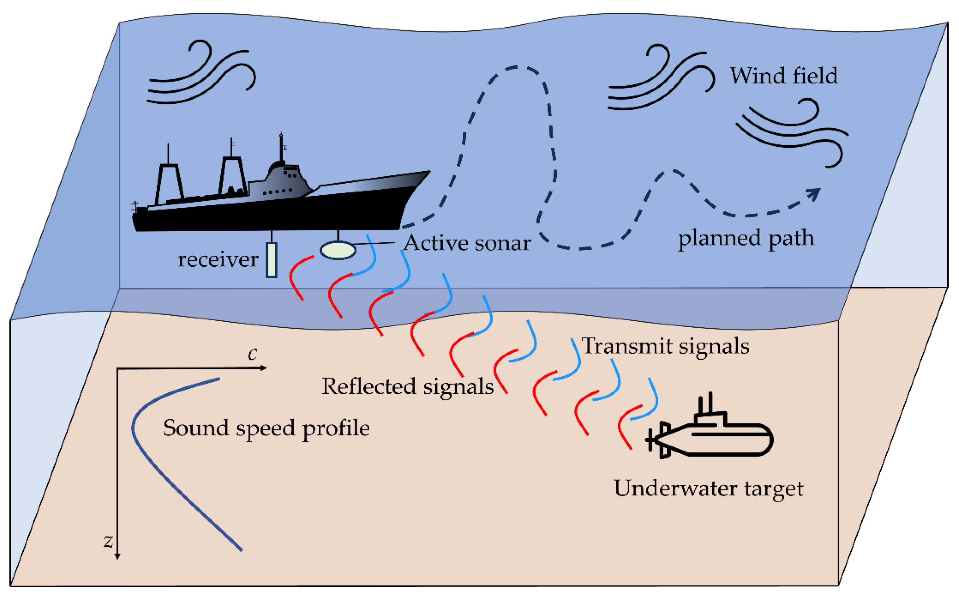
Figure 2.
Sixteen-azimuth path planning model.
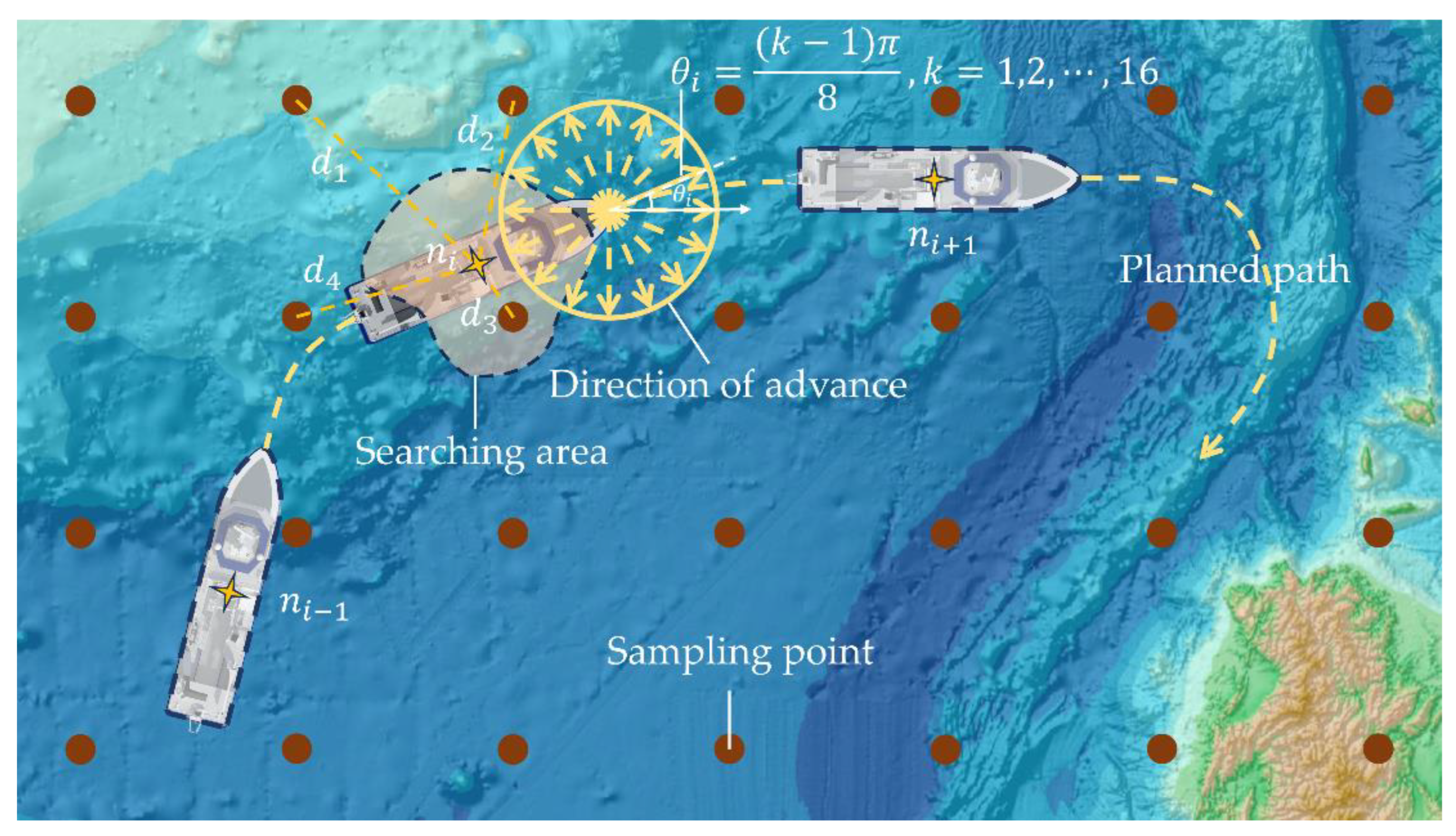
Figure 3.
Schematic diagram of mission sea areas.
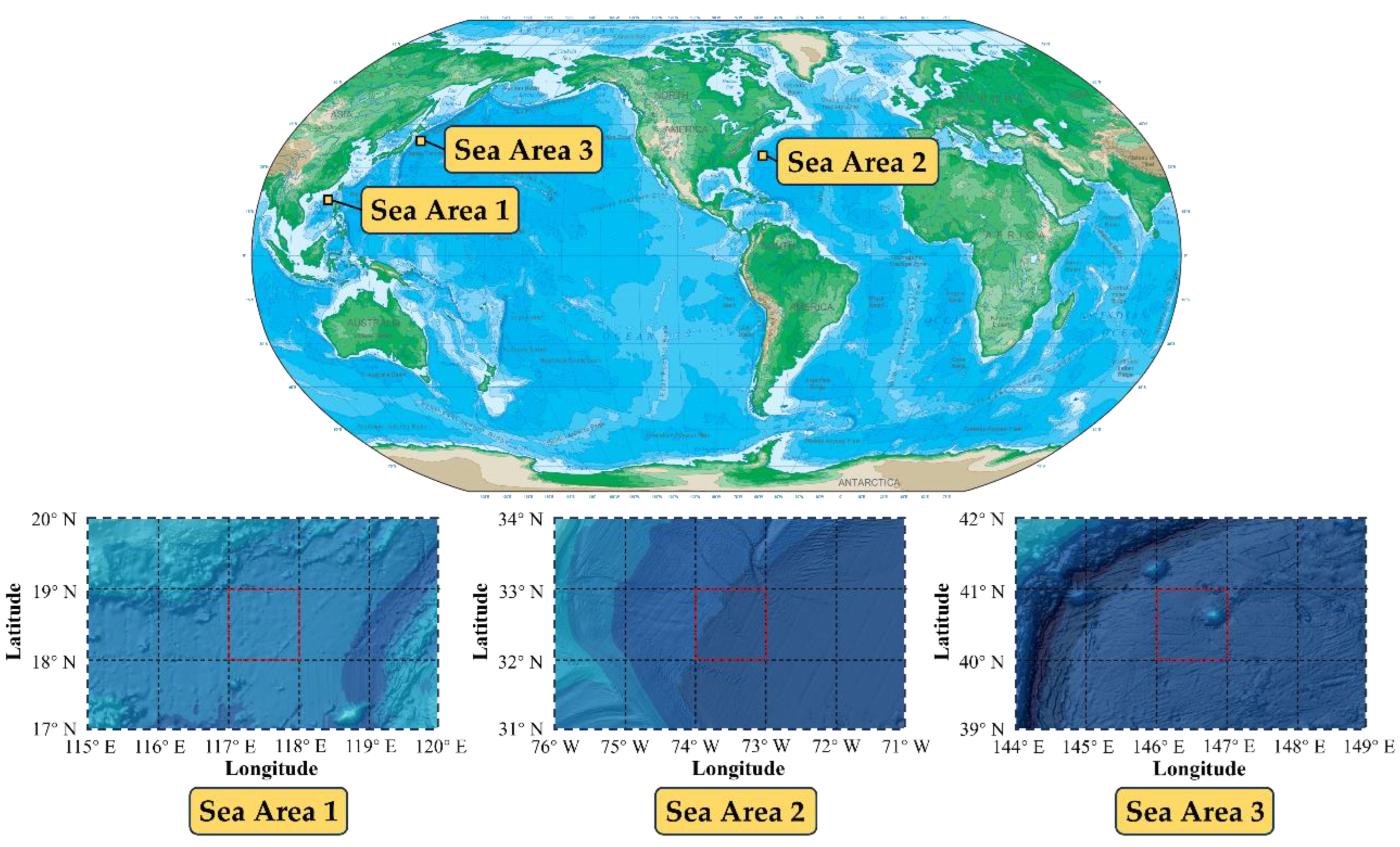
Figure 4.
Sound speed profiles. (a) Sea area 1; (b) Sea area 2; (c) Sea area 3.
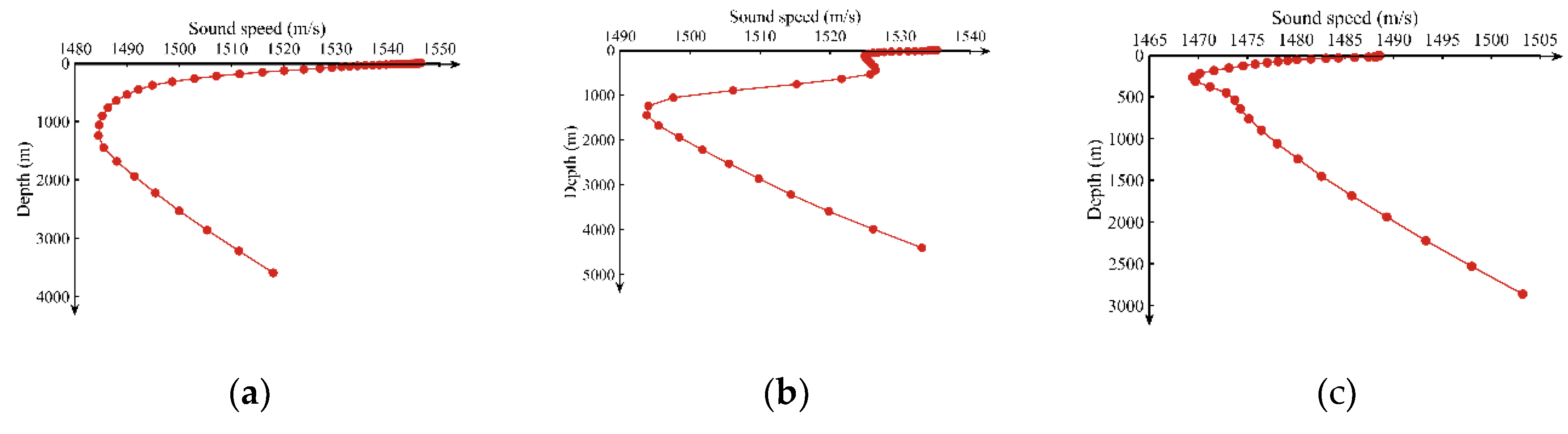
Figure 5.
Spatial distribution of NL. (a) Sea area 1; (b) Sea area 2; (c) Sea area 3.
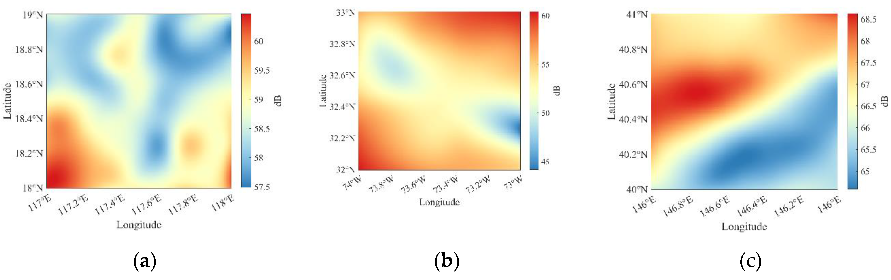
Figure 6.
Spatial distribution of active sonar search distance. (a) Sea area 1; (b) Sea area 2; (c) Sea area 3.
Figure 6.
Spatial distribution of active sonar search distance. (a) Sea area 1; (b) Sea area 2; (c) Sea area 3.

Figure 7.
Search paths before optimization. (a) Sea area 1; (b) Sea area 2; (c) Sea area 3.
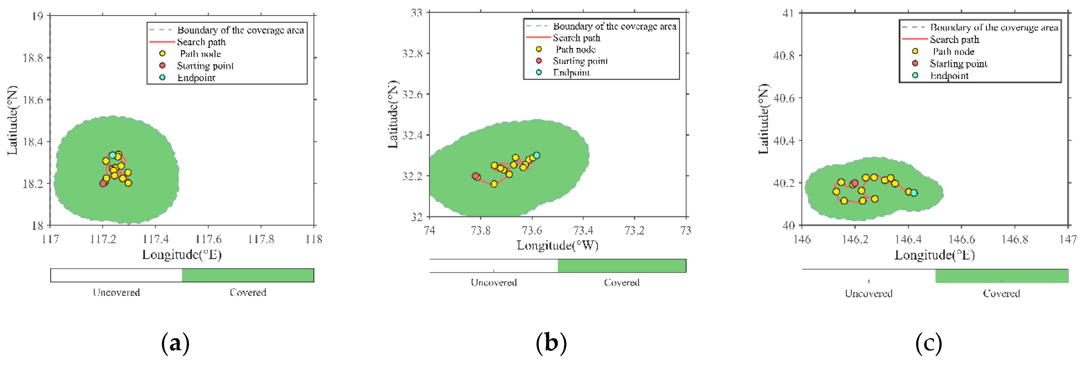
Figure 8.
Optimized search paths (Sea Area 1). (a) Path 1; (b) Path 2; (c) Path 3.
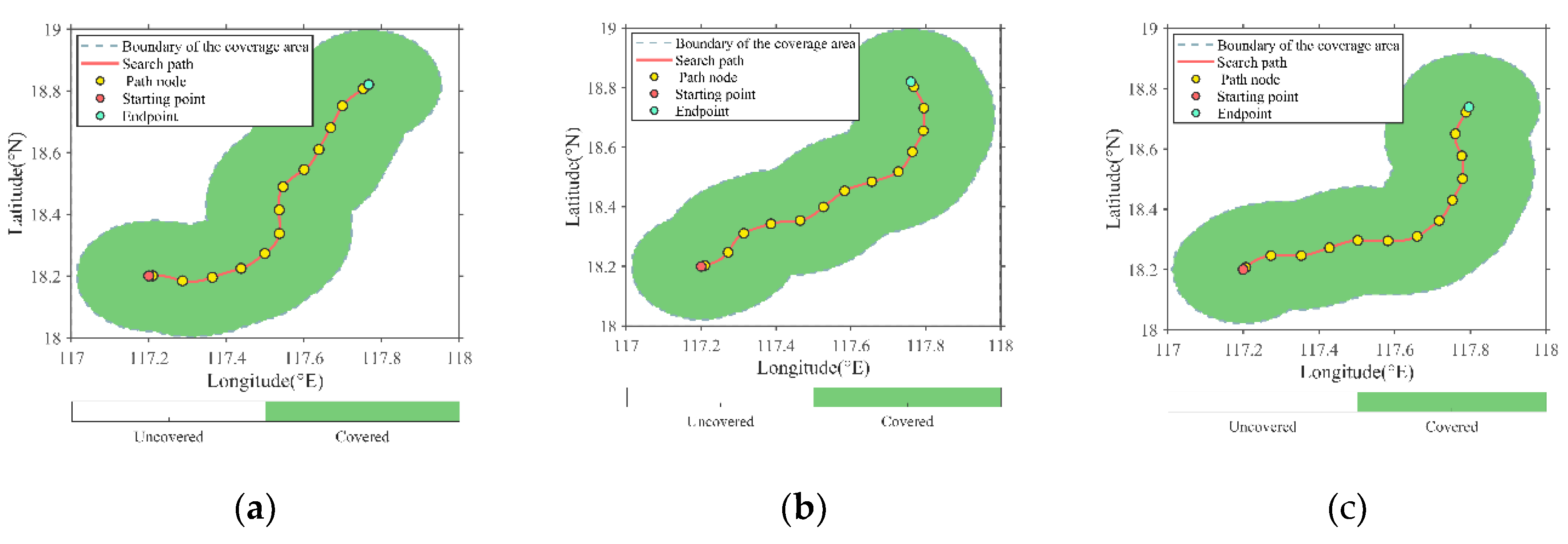
Figure 9.
Optimized search paths (Sea Area 2). (a) Path 1; (b) Path 2; (c) Path 3.
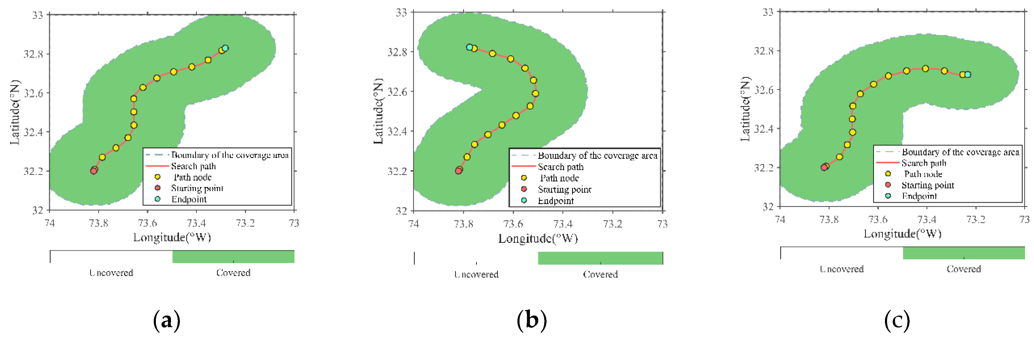
Figure 10.
Optimized search paths (Sea Area 3). (a) Path 1; (b) Path 2; (c) Path 3.
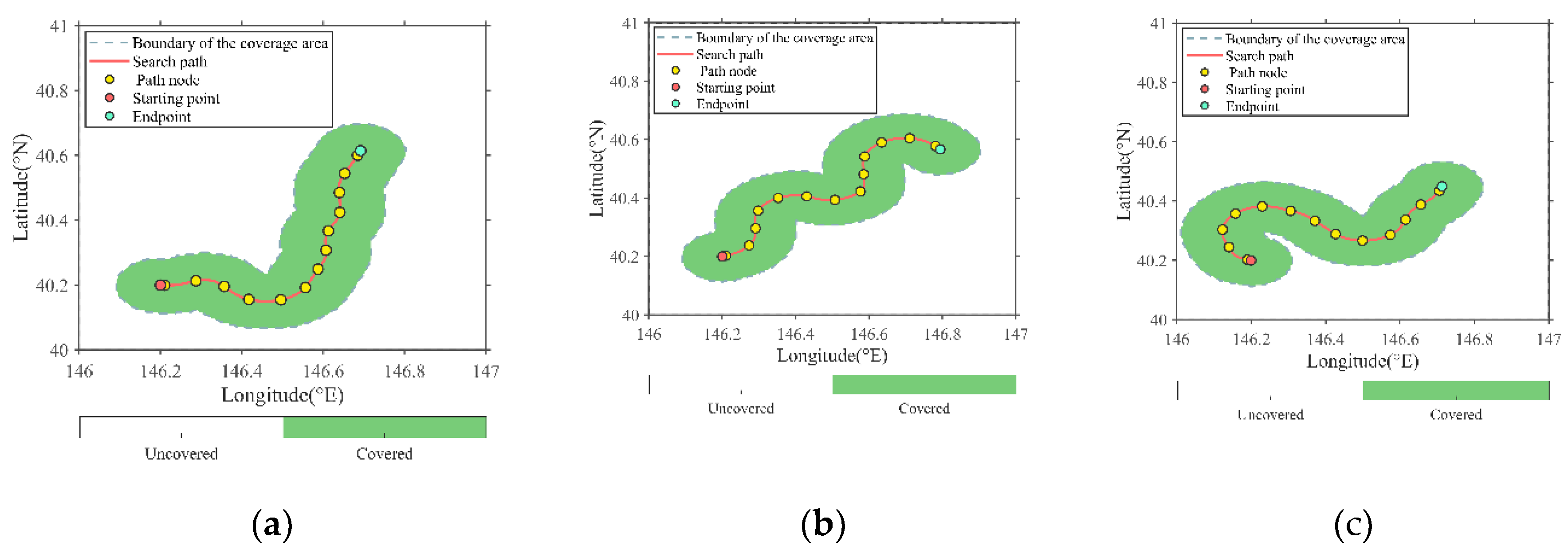
Figure 11.
Convergence curves and maximum coverage area of four algorithms (Sea Area 1). (a) Convergence curves; (b) Maximum search coverage area.
Figure 11.
Convergence curves and maximum coverage area of four algorithms (Sea Area 1). (a) Convergence curves; (b) Maximum search coverage area.
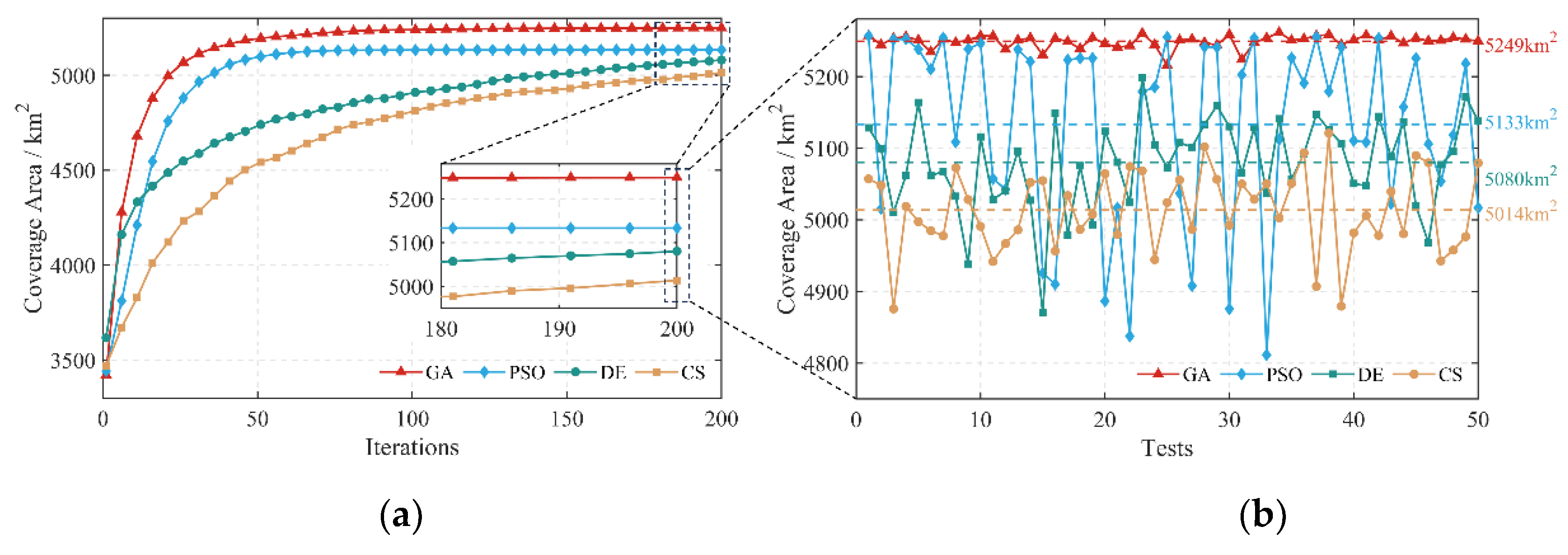
Figure 12.
Convergence curves and maximum coverage area of four algorithms (Sea Area 2). (a) Convergence curves; (b) Maximum search coverage area.
Figure 12.
Convergence curves and maximum coverage area of four algorithms (Sea Area 2). (a) Convergence curves; (b) Maximum search coverage area.
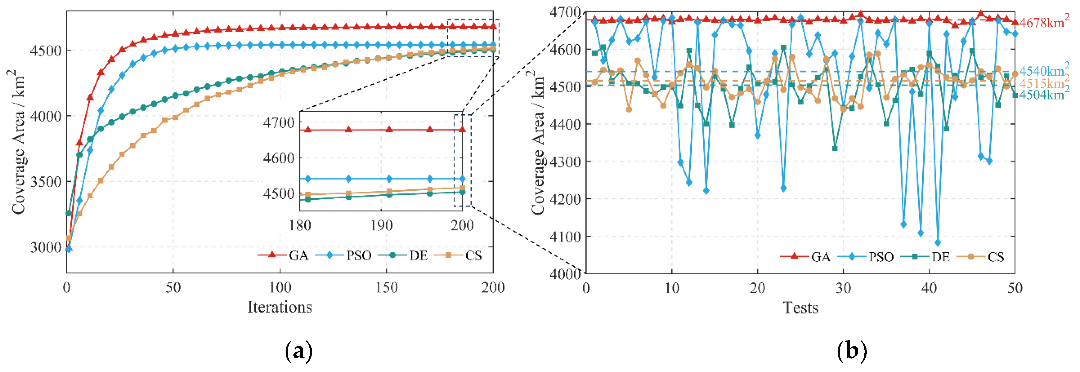
Figure 13.
Convergence curves and maximum coverage area of four algorithms (Sea Area 3). (a) Convergence curves; (b) Maximum search coverage area.
Figure 13.
Convergence curves and maximum coverage area of four algorithms (Sea Area 3). (a) Convergence curves; (b) Maximum search coverage area.
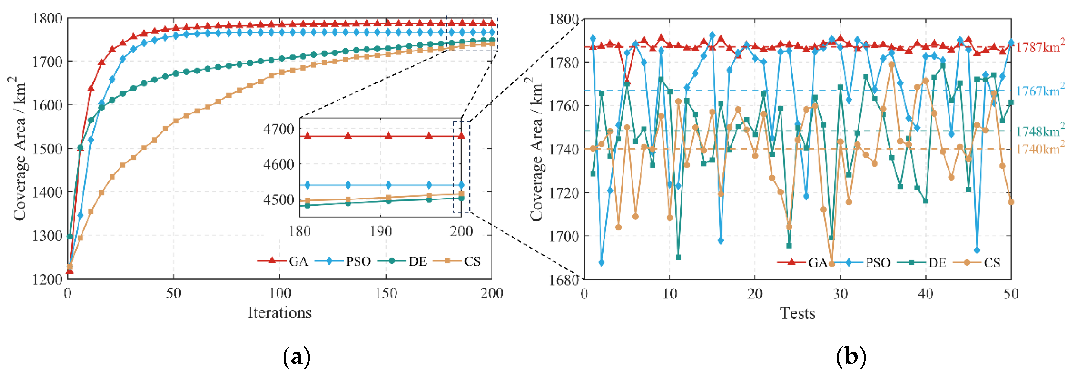
Figure 14.
Time consumption of four algorithms in 50 independent repeated experiments. (a) Sea area 1; (b) Sea area 2; (c) Sea area 3.
Figure 14.
Time consumption of four algorithms in 50 independent repeated experiments. (a) Sea area 1; (b) Sea area 2; (c) Sea area 3.
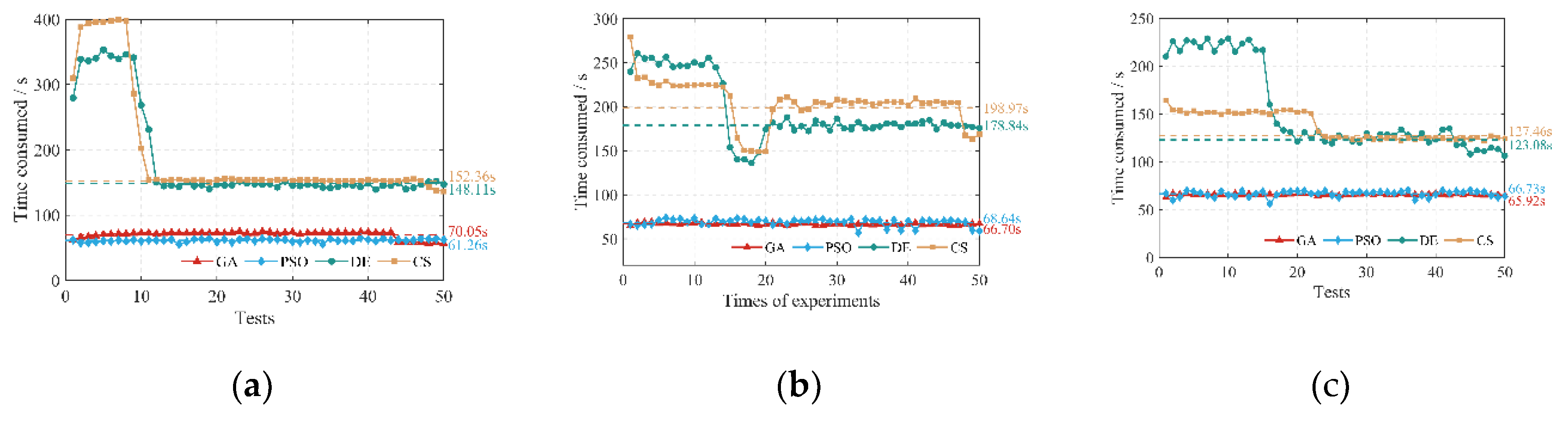

Table 1.
Average single calculation time of four algorithms (s).
| Mission sea areas | GA | PSO | DE | CS |
| Sea area 1 | 70.05 | 61.26 | 148.11 | 152.36 |
| Sea area 2 | 66.70 | 68.64 | 178.84 | 198.97 |
| Sea area 3 | 65.92 | 66.73 | 123.08 | 127.46 |
Table 2.
Average single calculation time of four algorithms (s).
| Mission sea areas | g | GA | PSO | DE | CS |
| Sea area 1 | 65% | 0.381 | 0.332 | 0.791 | 0.923 |
| 70% | 1.011 | 0.717 | 1.596 | 6.463 | |
| 75% | 1.341 | 1.063 | 3.192 | 12.948 | |
| 80% | 2.020 | 1.496 | 5.606 | 23.211 | |
| 85% | 3.042 | 2.196 | 16.401 | 40.134 | |
| 90% | 4.066 | 3.506 | 42.791 | 73.360 | |
| 95% | 7.177 | 6.817 | 118.733 | 178.301 | |
| Sea area 2 | 65% | 0.663 | 0.709 | 0.834 | 0.978 |
| 70% | 0.971 | 0.957 | 1.686 | 6.791 | |
| 75% | 1.290 | 1.409 | 3.394 | 16.549 | |
| 80% | 1.933 | 1.941 | 6.844 | 28.172 | |
| 85% | 2.916 | 2.786 | 22.163 | 46.098 | |
| 90% | 4.222 | 4.375 | 57.741 | 82.462 | |
| 95% | 7.517 | 9.172 | 146.598 | 154.811 | |
| Sea area 3 | 65% | 0.359 | 0.364 | 0.639 | 0.658 |
| 70% | 0.663 | 0.689 | 0.639 | 2.606 | |
| 75% | 0.969 | 0.812 | 1.287 | 6.529 | |
| 80% | 1.599 | 1.377 | 2.572 | 13.767 | |
| 85% | 2.234 | 1.713 | 4.550 | 27.078 | |
| 90% | 3.216 | 2.953 | 14.247 | 48.200 | |
| 95% | 5.507 | 5.374 | 65.999 | 84.462 |
Disclaimer/Publisher’s Note: The statements, opinions and data contained in all publications are solely those of the individual author(s) and contributor(s) and not of MDPI and/or the editor(s). MDPI and/or the editor(s) disclaim responsibility for any injury to people or property resulting from any ideas, methods, instructions or products referred to in the content. |
© 2025 by the authors. Licensee MDPI, Basel, Switzerland. This article is an open access article distributed under the terms and conditions of the Creative Commons Attribution (CC BY) license (http://creativecommons.org/licenses/by/4.0/).
Copyright: This open access article is published under a Creative Commons CC BY 4.0 license, which permit the free download, distribution, and reuse, provided that the author and preprint are cited in any reuse.


