Submitted:
19 June 2025
Posted:
20 June 2025
You are already at the latest version
Abstract
The conventional Bellhop ray model is constrained by its assumption of vertical stratification in sound speed, which limits its ability to accurately account for the deflection of ray trajectories caused by horizontal gradients in sound speed within the mixed layer. This limitation leads to inaccuracies in predicting convergence zone characteristics. This study introduces an enhanced ray model that incorporates the horizontal inhomogeneity of sound speed in the mixed layer, thereby enabling precise tracking of ray trajectories and accurate prediction of convergence zone characteristics. Experimental results demonstrate that, in comparison to the traditional Bellhop model, the proposed improved ray model reduces the prediction error of the distance to the first convergence zone in deep-sea environments by 2.26%. The enhanced model significantly enhances the accuracy of convergence zone characteristic predictions and can be effectively applied to the estimation of underwater acoustic detection ranges and the evaluation of sonar detection performance.
Keywords:
deep sea
; convergence zone
; characteristic forecasting
; ray model
1. Introduction
The convergence zone represents a distinctive acoustic propagation phenomenon within the deep-sea environment. This phenomenon is characterized by a periodically focused acoustic energy structure, which facilitates the transmission of acoustic signals over extended distances with reduced attenuation, thereby significantly augmenting the operational efficacy of sonar detection systems [1]. Predicting the characteristic parameters of the deep-sea convergence zone necessitates an examination of its distance, width, and gain. Investigating these parameters enables underwater combat units to precisely understand the influence of convergence zone characteristics on equipment performance. This understanding provides a supplementary basis for decision-making in the formulation of detection maneuver strategies during deep-sea operations.
In contemporary research, the primary approach for predicting the characteristic parameters of convergence zones involves analyzing the propagation paths of acoustic rays through the development of acoustic field models [2,3,4,5,6]. Notably, the Bellhop ray acoustic field model, introduced by Porter and Bueker, serves as a prominent method for modeling acoustic fields in horizontally inhomogeneous environments [7]. This model has gained widespread application in recent years for examining acoustic propagation characteristics. For instance, Weishuai et al. utilized the Douglas-Peucker algorithm to extract oceanographic factors from a database and employed the BELLHOP ray tracing model to derive acoustic propagation characteristics, thereby offering a predictive tool for studying underwater acoustic propagation in oceanic front environments [8] . Similarly, Liu et al. utilized a three-dimensional ocean acoustic framework, integrating the MITgcm and BELLHOP ray model, to investigate the coupling effects of the Luzon cold vortex and tidal waves [9]. Additionally, Ma et al. applied the BELLHOP ray theory model to explore the acoustic field characteristics associated with a pair of cyclonic vortices and a typical anticyclonic vortex [10].
Moreover, there is still a significant discrepancy between predictions using traditional ray models and acoustic experimental observations [12,13]. Therefore, data-driven prediction methods have been widely applied. Yang et al. designed an intelligent convergence zone recognition algorithm based on convolutional neural networks [14]. By inputting sound speed profiles and acoustic propagation loss data, the algorithm automatically extracts the spatiotemporal characteristics of caustic zones and achieved synchronous prediction of convergence zone distance and width in the East China Sea experiment, significantly improving efficiency compared to traditional physical models. Xu et al. developed a convergence zone prediction model based on high-resolution ocean fronts and tested 24 machine learning algorithms using k-fold cross-validation [15]. Li et al. constructed a convergence zone parameter prediction model under the influence of mesoscale eddies by integrating numerical simulations and measured data in multiple dimensions [16]. Ibebuchi and Richman used an autoencoder neural network to encode nonlinear sea surface temperature patterns in the tropical Pacific to predict the Nino 3.4 index [17]. Xu et al.utilized physics-informed machine learning methods to identify and predict acoustic convergence zone characteristics of mesoscale eddies under limited data conditions [18]. However, data-driven prediction methods struggle to cover multi-spatiotemporal scale acoustic-ocean joint datasets and face dual challenges of data quality and model interpretability due to their opaque physical mechanisms.
The actual marine environment is highly spatially heterogeneous and dynamically complex. Sound speed profiles are not uniformly distributed but are influenced by factors such as temperature and salinity, exhibiting significant horizontal gradient characteristics [19]. Particularly in the upper ocean (mixed layer), due to the effects of solar radiation, seasonal temperature differences, and ocean current shearing, sound speed profiles often show strong inhomogeneity [20]. Neither traditional ray models nor data-driven prediction methods have fully considered the horizontal inhomogeneity of sound speed in the deep-sea mixed layer, resulting in cumulative offsets in ray trajectories and directly affecting the prediction accuracy of convergence zone distance and width.
In this article, a horizontal sound speed gradient term is introduced into the ray equation, and a fourth-order Runge-Kutta numerical solution algorithm is designed. This breakthrough overcomes the limitation of traditional ray models that cannot represent the influence of horizontal sound speed gradients, thereby improving the prediction accuracy of convergence zone ray trajectories. The main innovations are as follows.
- A method for constructing horizontally inhomogeneous sound speed profiles in the deep-sea mixed layer is proposed. By using EOF decomposition technology to extract the spatial modal characteristics of temperature and salinity fields and combining them with the Del Grosso formula, a three-dimensional continuous sound speed field is generated. This approach overcomes the limitation of traditional models that simplify mixed layer sound speed as vertically stratified, achieving dynamic coupled modeling of sound speed profiles with horizontal distance and vertical depth.
- An improved ray tracing algorithm based on non-uniformly distributed sound speed profiles is developed. By introducing the horizontal sound speed gradient term into the ray equation and designing a fourth-order Runge-Kutta numerical solution algorithm, the bottleneck of traditional ray models in representing the influence of horizontal sound speed gradients is overcome, thereby improving the prediction accuracy of convergence zone ray trajectories.
- The enhanced algorithm for forecasting convergence zone characteristic parameters was validated using environmental parameters from a representative marine area. The findings indicate that the refined ray model successfully accounted for the forward displacement of the convergence zone induced by the horizontal gradient of sound speed within the mixed layer, thereby enhancing the forecast’s accuracy.
The rest of the article is organized as follows. Section 2 is the analysis of the non-uniform sound speed profile in the deep-sea mixed layer. Section 3 is the forecast of convergence zone characteristic parameters based on an improved ray model. Section 4 is the simulation. Section 5 is the conclusion.
2. Analysis of the Non-uniform Sound Speed Profile in the Deep-sea Mixed Layer
This article constructs a non-uniform sound speed profile model for the mixed layer by measuring temperature, salinity, and pressure data and substituting them into empirical formulas [21,22]. Firstly, the driving factors of sound speed in the mixed layer are analyzed from the perspective of physical mechanisms. It is clarified that the horizontal gradients of the temperature and salinity fields are the main sources of spatial heterogeneity of sound speed, while the pressure field dominates the vertical stratification structure through the hydrostatic effect. Secondly, within the framework of the classical Del Grosso sound speed formula [23], the temperature and salinity parameters are decomposed into coupled functions of horizontal distance and vertical depth using gridded measured temperature, salinity, and pressure data, thereby establishing the non-uniform distribution relationship of sound speed with horizontal distance and vertical depth within the mixed layer of the sea area. Finally, the mixed layer depth is introduced as a boundary threshold to construct a piecewise continuous sound speed profile model. The steps are shown in Figure 1.
2.1. Analysis of Factors Affecting Sound Speed in the Mixed Layer
This section employs the empirical formulae for ocean sound velocity calculation [23,24,25], to analyze the impact mechanisms of the mixed layer sound velocity from the perspective of physical mechanisms, which are shown in equation (1), (2) and (3):
where C and V represent the sound speed, T is the temperature of sea, S is the salinity of sea, Z is depth and P is pressure. According to the theory of the wave equation, sound speed refers to the phase velocity of a plane wave, which is a longitudinal wave and is related to density and compressibility. It can be expressed as:
where and represent The density and adiabatic compressibility of seawater.
2.1.1. The Effection of Temperature on Sound Speed
Based on the functional relationship between the compressibility of seawater and the temperature field, an empirical relationship model was established using marine observational data [26]:
Let , , then we have
Within the typical fluctuation range of conventional marine environmental parameters, the variation in density is minimal. By adopting the assumption of approximate constancy, we have
where represents the sound speed at a temperature of C.
By applying the Taylor series expansion method to linearize the above equation and retaining the first and second-order terms to construct a simplified model, then we have
The expression for the change in sound speed derived through this model is
Equation(9) indicates that when the temperature changes by C, the relative increase in sound speed is approximately 0.354% of the original value.
2.1.2. The Effection of Salinity on Sound Speed
According to the empirical formula between seawater density and salinity [26], we have
where S represents salinity. The relationship between the compressibility coefficient of seawater and salinity can be expressed as
From equation (10) and equation (11), it can be seen that When the salinity increases by 1, the compressibility decreases by 0.24%, and the sound speed increases; when the density increases by 0.08%, the sound speed decreases. Substituting equation (10) and equation (11) into equation (4), we have
Substituting and into equation (12) , we have
From equation (13), it can be concluded that when salinity increases by 1, the relative increase in sound speed is approximately 0.0825% of the original value.
2.1.3. The Effect of Pressure on the Speed of Sound
The change in sound speed due to pressure mainly depends on the variation of the compressibility coefficient . For seawater, the greater the pressure, the more difficult it is to compress, and the smaller the compressibility coefficient becomes, which ultimately leads to an increase in sound speed. Therefore, pressure is positively correlated with sound speed. The following is the expression for the relationship between the static pressure of seawater and the compressibility coefficient:
where the pressure is measured in units of one standard atmosphere (101325 Pa). Substituting equation (14) into equation (4), the change in sound speed is finally obtained as
As can be seen from equation (15), when the pressure increases by 1 Pa, the relative increase rate of sound speed is approximately 0.022% of its original value.
2.2. Construction of Non-uniform Sound Speed Profiles
This section elaborates on the data-driven method for constructing non-uniform sound speed profiles, including data acquisition and processing, modeling of the horizontal-vertical distribution of temperature and salinity, and Del Grosso sound speed coupling analysis.
2.2.1. Data Acquisition and Preprocessing
The data source used in this article is the ocean space temperature, salinity, and pressure data, which is derived from the global ocean Argo gridded data set (BOA_Argo) provided by the Argo Real-Time Data Center [27]. The data applied include longitude, latitude, pressure, salinity, temperature, and mixed layer depth. Taking temperature as an example, its surface distribution is shown in Figure 2(a). After obtaining the measured data, the data are preprocessed by regional clipping according to the research sea area. The index corresponding to longitude is obtained through the following minimization formula, and the same applies to latitude j. The final longitude and latitude index ranges are determined as and , and the clipped sea area is shown in Figure 2(b).
2.2.2. Modeling the horizontal and vertical distribution of temperature and salinity
To accurately characterize the continuous spatial distribution of temperature, salinity, and pressure, this article employs a two-dimensional Empirical Orthogonal Function (EOF) decomposition method, combined with measured data and function interpolation techniques, to construct a temperature field parameterization model [28]. The original temperature and salinity data have a horizontal resolution of , and are vertically divided at 10m intervals within the mixed layer. The data are preprocessed to eliminate the dimensional differences in the vertical stratification and to highlight the spatial characteristics of the temperature and salinity fields. Each depth layer of the temperature and salinity fields is normalized.
Based on the BOA_Argo data, the horizontal-vertical distribution model of temperature and salinity established using EOF and the comparison with the original data are shown in Figure 3.
2.2.3. Del Grosso acoustic velocity coupling
Considering the horizontal inhomogeneity of the sound speed profile in the deep-sea mixed layer, the sound speed profile is described in segments. The entire sound speed profile can be represented by the following equation:
where, r represents the horizontal distance, z represents the vertical depth, represents the depth of the mixed layer, and H represents the sea depth. When , the sound speed profile will fluctuate with changes in horizontal distance and vertical depth, exhibiting non-uniform distribution characteristics. When , the sound speed is located below the mixed layer and varies only with depth. The schematic diagram of the sound speed profile is shown in Figure 4, with the mixed layer above the stratification line. The solid line represents the simplified equivalent sound speed profile that ignores the non-uniform changes in the marine environment, and the shaded area represents the fluctuation range caused by the non-uniform distribution of sound speed.
The Del Grosso algorithm, as shown in equation (1). To ensure the continuity of the sound speed profile at , the function C in equation (16) must satisfies .
The temperature and salinity at the base of the mixed layer must smoothly transition to the deep-layer constant values, which is specifically realized by introducing the transition function :
where is a cubic polynomial weighting function:
To avoid a significant impact on the sound speed, the thickness of the transition layer, , is set to only 2-5m, to ensure the continuity of the first-order derivative of the sound speed. In this case, the temperature gradient at the base of the mixed layer, , and the salinity gradient, , will smoothly decay to zero, avoiding the occurrence of a sawtooth discontinuity in the sound speed at the boundary point.
3. Forecast of Convergence Zone Characteristic Parameters Based on an Improved Ray Model
3.1. Ray model improvement
Starting from the classical ray equation, this section derives the improved ray tracing equation for non-uniform media, designs a numerical solution algorithm, and clarifies the implementation process of the improved model in the prediction of parameters in the convergence zone. According to the eikonal equation, the ray direction is defined as the normal direction of the wavefront, where the wavefront is the set of points with the same acoustic pressure vibration phase. The normal direction at any point on the wavefront is the direction of the phase gradient at that point, representing the direction of sound wave propagation, that is:
Combining the eikonal equation , we have
Differentiate with respect to s, using the chain rule, we have
after expanding equation(20), we obtain that
In the two-dimensional vertical plane (horizontal x, vertical z), let the angle between the sound ray and the horizontal plane be , then we have
Differentiate with respect to , using the geometric relationship, we have
Finally, we obtain the differential equation system describing the sound ray trajectory in the traditional ray model by equation (19) – (24):
In the equation, s is the arc length of the sound ray, is the angle between the sound ray and the horizontal plane, and is the vertically stratified sound speed. This model does not consider the effect of the horizontal gradient term of the sound speed .
Considering the non-uniform sound speed profile that depends on both the horizontal position r and depth z, the ray model is improved starting from the eikonal equation, and the model must include the horizontal gradient term . The propagation of sound waves can be regarded as particles moving along ray trajectories. Therefore, starting from the Hamiltonian mechanics framework, the ray tracing problem is transformed into a particle trajectory problem in classical mechanics. The position coordinates are defined as and the momentum as , with the Hamiltonian [29]
The equations of motion in Hamiltonian mechanics are:
After expanding equation (27) and using equation (26), the canonical equation that the ray trajectory satisfies:
From the eikonal equation , the physical meaning of the momentum is the direction of the wave vector. Combining this with the sound ray direction angle , we can write and . Through variable substitution, we obtain the improved ray equation system:
Compared with the classical equation (25), the added term in equation (29) quantifies the contribution of the horizontal gradient to the curvature of the sound ray. When , the sound ray will deflect towards the direction of increasing sound speed, resulting in a lateral displacement of the propagation path, as shown in Figure 5.
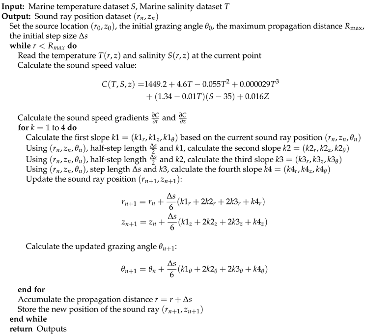
The complexity of the improved ray-tracing algorithm makes the equations analytically intractable, necessitating the use of numerical methods. This article employes the fourth-order Runge-Kutta method (RK4) to numerically integrate the improved ray equations. The pseudocode for its algorithm implementation is shown as Algorithm 1.
3.2. Forecast of Convergence Zone Characteristic Parameters
The construction of sound rays in the acoustic field is achieved using the Bellhop acoustic toolbox in Matlab, which further enables the calculation of the distance, width, and gain of the first convergence zone. The subsequent rows contain the actual sound speed values, in meters per second, with each row corresponding to a fixed depth. The actual depths used are taken from the depth data below the fifth line in the environmental file.
When analyzing specific sea areas, bathymetric data can be obtained from the General Bathymetric Chart of the Oceans (GEBCO) database [30]. The plotssp2d command is used to draw the horizontal inhomogeneous distribution of sound speed profiles in the mixed layer. The resulting sound speed profile curves associated with horizontal distance and vertical depth, as well as the color-mapped sound speed profile images, are shown in Figure 6(a) and Figure 6(b), respectively. The plotray command is used to track sound rays and generate the sound field model of the convergence zone, as shown in Figure 6(c). It can be seen that the sound rays in the convergence zone, considering the horizontally inhomogeneous sound speed profile, exhibit significant fluctuations compared to those under the typical Munk profile during propagation. The overall shape of the sound rays is more complex and clearly conforms more closely to the actual sound signal propagation patterns. Based on this, the prediction of the distance and width of the first convergence zone is consistent with the method under the typical Munk profile and can be easily calculated by measuring the upper bending point of the sound ray with a launch angle and the critical depth bending sound ray. The prediction of the gain in the first convergence zone is also calculated by constructing a transmission loss model, as shown in Fig. Figure 6(d).
4. Simulation
In this section, the acoustic propagation characteristic experiment conducted in the South China Sea in 2018 is selected as the benchmark case data.
4.1. Characteristic Features of Typical Marine Environment and Data Preparation
The typical sea area selected for the simulation experiment of the convergence zone characteristic parameter forecasting algorithm is covered by the sea area of the 2018 spring South China Sea acoustic propagation experiment. The selected area is located at N latitude and E-E longitude in the South China Sea, with a depth of approximately 3500 meters and a horizontal distance of about 110 kilometers. The environmental characteristic data include temperature, salinity, pressure, and mixed layer depth. The temperature and salinity profiles are shown in Figure 7.
| Algorithm 1 Improved sound ray tracing algorithm for the ray model. |
 |
In the South China Sea experiment, the source depth was 80 m and the source frequency was 300 Hz. The convergence zone characteristic parameters obtained using the first-order internal wave normal mode basis function model are shown in Table 1, which will be used to verify the accuracy of the Bellhop ray model and the improved ray model in predicting convergence zone characteristics.
4.2. Simulation of Convergence Zone Characteristic Parameter Forecasting and Comparative Analysis of Results
The temperature, salinity, and depth data of the typical sea area are substituted into the empirical sound speed formula of Del Grosso. The sound speed profile is then written into the environmental file to generate a simplified equivalent sound speed profile for the entire sea area under the traditional ray model, as shown in Figure 8.
Under the Bellhop ray model, the simple equivalent sound speed profile is relatively smooth. The mixed layer does not take into account the horizontal distance. The sound channel axis is located at a depth of about 800 meters. The minimum sound speed is 1496.74 m/s, the sea surface sound speed is 1515.9 m/s, and the sea bottom sound speed is 1518.67 m/s. Under this sound speed profile, there is a convergence zone effect.
Combining the temperature, salinity, and depth data with the latitude and longitude data of typical sea areas, a horizontal-vertical distribution model of the temperature-salinity field was constructed using the two-dimensional empirical orthogonal functions. By coupling the Del Grosso empirical formula for sound speed, the horizontally non-uniform sound speed profiles in the mixed layer were obtained, as shown in Figure 9 and Figure 10.
Figure 9 shows that the sound speed profile changes with horizontal distance due to the mixed layer’s temperature and salinity inhomogeneity. At the sea surface, sound speed is 1515.86 m/s at E, 1517.65 m/s at E, and 1519.67 m/s at E, while it is nearly constant below the mixed layer. This is because the mixed layer’s temperature and salinity increase with distance, but remain constant below it. The color mapping of sound speed also shows that the mixed layer’s sound speed rises with distance. Although the sound speed considering the mixed layer’s non-uniformity differs from the simple equivalent sound speed, their overall trends are similar, with the sound channel axis depth around 800 m. This confirms the effectiveness of the improved sound speed profile.
Based on the construction of the sound speed profile, the acoustic propagation paths under the Bellhop ray model and the improved ray model are simulated. According to the experimental scenario, the source depth is set to 80 m, the source frequency is set to 300 Hz, and the emission angle range is set to . The sound rays of the sound field drawn by the Bellhop ray model and the improved ray model are shown in Figure 11.
The improved ray model sound field shifts significantly forward compared to the Bellhop ray model sound field. This is due to the consideration of the horizontally inhomogeneous sound speed distribution, which changes the turning points of the sound rays. Specifically, the turning point depth of rays with smaller emission angles becomes shallower, while that of rays with larger emission angles becomes deeper. The upper turning points of the emission angle ray and the critical depth bending ray are shown in Figure 12.
It can be seen that, according to the Bellhop ray model, the distance to the first convergence zone is 63.6742 km, and the width of the first convergence zone is 20.1763 km; according to the improved ray model, the distance to the first convergence zone is 60.7144 km, and the width of the first convergence zone is 20.7463 km.
The first convergence zone gain is obtained by plotting the propagation loss model. The magnitude of the propagation loss varies with the receiver location. Therefore, according to the experimental setup, the receiver is placed at a depth of 200 meters within the convergence zone distance to measure the magnitude of the convergence zone gain. The propagation loss models of the Bellhop ray model and the improved ray model are shown in Figure 13.
The Bellhop ray model shows a propagation loss of about 93 dB outside the convergence zone and a minimum loss of 77.8827 dB inside it, giving a convergence zone gain of around 15.12 dB. The improved ray model has a propagation loss of about 90 dB outside the convergence zone and a minimum loss of 77.334 dB inside, resulting in a gain of about 12.67 dB. Thus, the convergence zone gain from the Bellhop model is slightly higher than that from the improved model. Compare the prediction results of the characteristics parameters of the first convergence zone by the Bellhop ray model and the improved ray model with the experimental results, as shown in Table 2.
The comparison shows that the improved ray model has enhanced the accuracy of the first convergence zone distance prediction by 2.26%, the first convergence zone width prediction by 2.66%, and the first convergence zone gain prediction by approximately 5.85% compared with the Bellhop ray model, which demonstrates the effectiveness of the improvements made to the ray model in this article.
5. Conclusion
This article proposes an improved ray model framework that constructs a sound speed profile model with horizontal gradient corrections by integrating real measured ocean environmental data, and verifies its effectiveness. The model significantly enhances the prediction accuracy of deep-sea convergence zone characteristic parameters, effectively addressing the forecast deviation caused by traditional models ignoring the horizontal inhomogeneity of sound speed in the mixed layer. Future research will employ machinoee learning methods to further improve the prediction capability of convergence zone acoustic field effects and apply it to practical mission scenarios, thereby promoting the development of underwater detection and communication technologies.
Author Contributions
Conceptualization, Guangyu Luo and Dongming Zhao; Data curation, Hao Zhou; Formal analysis, Hanyi Wang; Funding acquisition, Xuan Guo; Investigation, Heng Fang; Methodology, Hao Zhou; Project administration, Dongming Zhao; Resources, Guangyu Luo; Software, Xuan Guo; Supervision, Kai Xia; Validation, Hanyi Wang, Caihua Fang and Kai Xia; Visualization, Heng Fang; Writing – original draft, Guangyu Luo; Writing – review & editing, Dongming Zhao. All authors will be updated at each stage of manuscript processing, including submission, revision, and revision reminder, via emails from our system or the assigned Assistant Editor.
Funding
This research was funded by the China Postdoctoral Science Foundation under Grant Number 2024M752505.
Data Availability Statement
Data will be made available on request.
Conflicts of Interest
The authors declare no conflicts of interest.
References
- Zhao, D.; Liang, S.; Chen, P.; Hu, Y.; Dang, Y.; Li, Y.; Liang, R.; Guo, X. Design of Deep-Sea Imaging Sonar System With Universal-Scene Sparse Array. IEEE Transactions on Instrumentation and Measurement 2025. [Google Scholar] [CrossRef]
- Li, Y.; Jia, N.; Huang, J.; Han, R.; Guo, Z.; Guo, S. Analysis of High-Frequency Communication Channel Characteristics in a Typical Deep-Sea Incomplete Sound Channel. Electronics 2023, 12, 4562. [Google Scholar] [CrossRef]
- Papkova, Y.I. Sound Fields in Marine Waveguides with a Heterogeneous Speed of Sound Along the Depth and Path. Moscow University Physics Bulletin 2021, 76, 157–166. [Google Scholar] [CrossRef]
- Bhatt, E.C.; Baggeroer, A.B.; Weller, R.A. Overflow waters in the western Irminger Sea modify deep sound speed structure and convergence zone propagation. The Journal of the Acoustical Society of America 2024, 155, 1216–1229. [Google Scholar] [CrossRef]
- Wu, S.; Li, Z.; Qin, J.; Wang, M.; Li, W. The effects of sound speed profile to the convergence zone in deep water. Journal of Marine Science and Engineering 2022, 10, 424. [Google Scholar] [CrossRef]
- Shu-Qing, M.; Xiao-Jin, G.; Li-Lun, Z.; Qiang, L.; Chuang-Xia, H. Riemannian geometric modeling of underwater acoustic ray propagation? application–Riemannian geometric model of convergence zone in deep ocean remote sound propagation br. ACTA PHYSICA SINICA 2023, 72. [Google Scholar]
- Porter, M.B.; Bucker, H.P. Gaussian beam tracing for computing ocean acoustic fields. The Journal of the Acoustical Society of America 1987, 82, 1349–1359. [Google Scholar] [CrossRef]
- Weishuai, X.; Zhang, L.; Hua, W. The Influential Factors and Prediction of Kuroshio Extension Front on Acoustic Propagation-Tracked. Archives of Acoustics 2023, 49, 95–106. [Google Scholar]
- Liu, Y.; Zhang, X.; Fu, H.; Qian, Z. Response of sound propagation characteristics to Luzon cold eddy coupled with tide in the Northern South China Sea. Frontiers in Marine Science 2023, 10, 1278333. [Google Scholar] [CrossRef]
- Ma, X.; Zhang, L.; Xu, W.; Li, M. Analysis of acoustic field characteristics of mesoscale eddies throughout their complete life cycle. Frontiers in Marine Science 2025, 11, 1471670. [Google Scholar] [CrossRef]
- Cheng, C.; Zheng, C.; Hong, X. A deep-sea direct sound ranging method based on effective sound velocity estimation for turning ray. JASA Express Letters 2025, 5. [Google Scholar] [CrossRef]
- Talha, R.M.; Farooq, M.A.; Khan, S.; Iqbal, K.; Ismail, M.A. Development of Oceanographic Acoustic Modelling Tools for Streamlined Transmission Loss Analysis. In Proceedings of the 2024 21st International Bhurban Conference on Applied Sciences and Technology (IBCAST). IEEE; 2024; pp. 694–700. [Google Scholar]
- Peng, Z.; Zheng-Lin, L.; Li-Xin, W.; Ren-He, Z.; Ji-Xing, Q. Characteristics of convergence zone formed by bottom reflection in deep water. ACTA PHYSICA SINICA 2019, 68. [Google Scholar]
- Yang, Y.; Mao, Y.; Xie, R.; Hu, Y.; Nan, Y. A novel optimal route planning algorithm for searching on the sea. The Aeronautical Journal 2021, 125, 1064–1082. [Google Scholar] [CrossRef]
- Xu, W.; Zhang, L.; Wang, H. Machine learning–based feature prediction of convergence zones in ocean front environments. Frontiers in Marine Science 2024, 11, 1337234. [Google Scholar] [CrossRef]
- Li, M.; Liu, Y.; Sun, Y.; Liu, K. Quantitative analysis and prediction of the sound field convergence zone in mesoscale eddy environment based on data mining methods. Acta Oceanologica Sinica 2024, 43, 110–120. [Google Scholar] [CrossRef]
- Ibebuchi, C.C.; Richman, M.B. Deep learning with autoencoders and LSTM for ENSO forecasting. Climate Dynamics 2024, 62, 5683–5697. [Google Scholar] [CrossRef]
- Xu, W.; Zhang, L.; Li, M.; Ma, X.; Wang, H. A physics-informed machine learning approach for predicting acoustic convergence zone features from limited mesoscale eddy data. Frontiers in Marine Science 2024, 11, 1364884. [Google Scholar] [CrossRef]
- Zhang, W.; Jin, S.; Bian, G.; Peng, C.; Xia, H. A Method for Full-Depth Sound Speed Profile Reconstruction Based on Average Sound Speed Extrapolation. Journal of Marine Science and Engineering 2024, 12, 930. [Google Scholar] [CrossRef]
- Richards, E.L.; Colosi, J.A. Observations of ocean spice and isopycnal tilt sound-speed structures in the mixed layer and upper ocean and their impacts on acoustic propagation. The Journal of the Acoustical Society of America 2023, 154, 2154–2167. [Google Scholar] [CrossRef] [PubMed]
- Wu, P.; Sun, J.; Shan, G.; Sun, Z.; Wei, P. Inversion of deep-water velocity using the munk formula and the seabed reflection traveltime: an inversion scheme that takes the complex seabed topography into account. IEEE Transactions on Geoscience and Remote Sensing 2023, 61, 1–14. [Google Scholar] [CrossRef]
- Yang, F.; Hu, T.; Wang, Z. Effects of sound velocity perturbations in the upper layer on the position of sound convergence zones in deep water. In Proceedings of the 2021 OES China Ocean Acoustics (COA). IEEE; 2021; pp. 327–330. [Google Scholar]
- Del Grosso, V.A. New equation for the speed of sound in natural waters (with comparisons to other equations). The Journal of the Acoustical Society of America 1974, 56, 1084–1091. [Google Scholar] [CrossRef]
- Wilson, W.D. Extrapolation of the equation for the speed of sound in sea water. The Journal of the Acoustical Society of America 1962, 34, 866–866. [Google Scholar] [CrossRef]
- Kang, E.J.; Sohn, B.J.; Kim, S.W.; Kim, W.; Kwon, Y.C.; Kim, S.B.; Chun, H.W.; Liu, C. A revised ocean mixed layer model for better simulating the diurnal variation in ocean skin temperature. Geoscientific Model Development 2024, 17, 8553–8568. [Google Scholar] [CrossRef]
- McDougall, T.J.; Jackett, D.R.; Wright, D.G.; Feistel, R. Accurate and computationally efficient algorithms for potential temperature and density of seawater. Journal of Atmospheric and Oceanic Technology 2003, 20, 730–741. [Google Scholar] [CrossRef]
- Li, H.; Xu, F.; Zhou, W.; Wang, D.; Wright, J.S.; Liu, Z.; Lin, Y. Development of a global gridded A rgo data set with B arnes successive corrections. Journal of Geophysical Research: Oceans 2017, 122, 866–889. [Google Scholar] [CrossRef]
- Obled, C.; Creutin, J. Some developments in the use of empirical orthogonal functions for mapping meteorological fields. Journal of Applied Meteorology and Climatology 1986, 25, 1189–1204. [Google Scholar] [CrossRef]
- Koyanagi, S.; Nakano, T.; Kawabe, T. Application of Hamiltonian of ray motion to room acoustics. The Journal of the Acoustical Society of America 2008, 124, 719–722. [Google Scholar] [CrossRef]
- Zaki, A.; Bashir, B.; Alsalman, A.; Elsaka, B.; Abdallah, M.; El-Ashquer, M. Evaluating the Accuracy of Global Bathymetric Models in the Red Sea Using Shipborne Bathymetry. Journal of the Indian Society of Remote Sensing 2025, 53, 277–291. [Google Scholar] [CrossRef]
Figure 1.
The steps for analyzing the non-uniform sound speed profile.
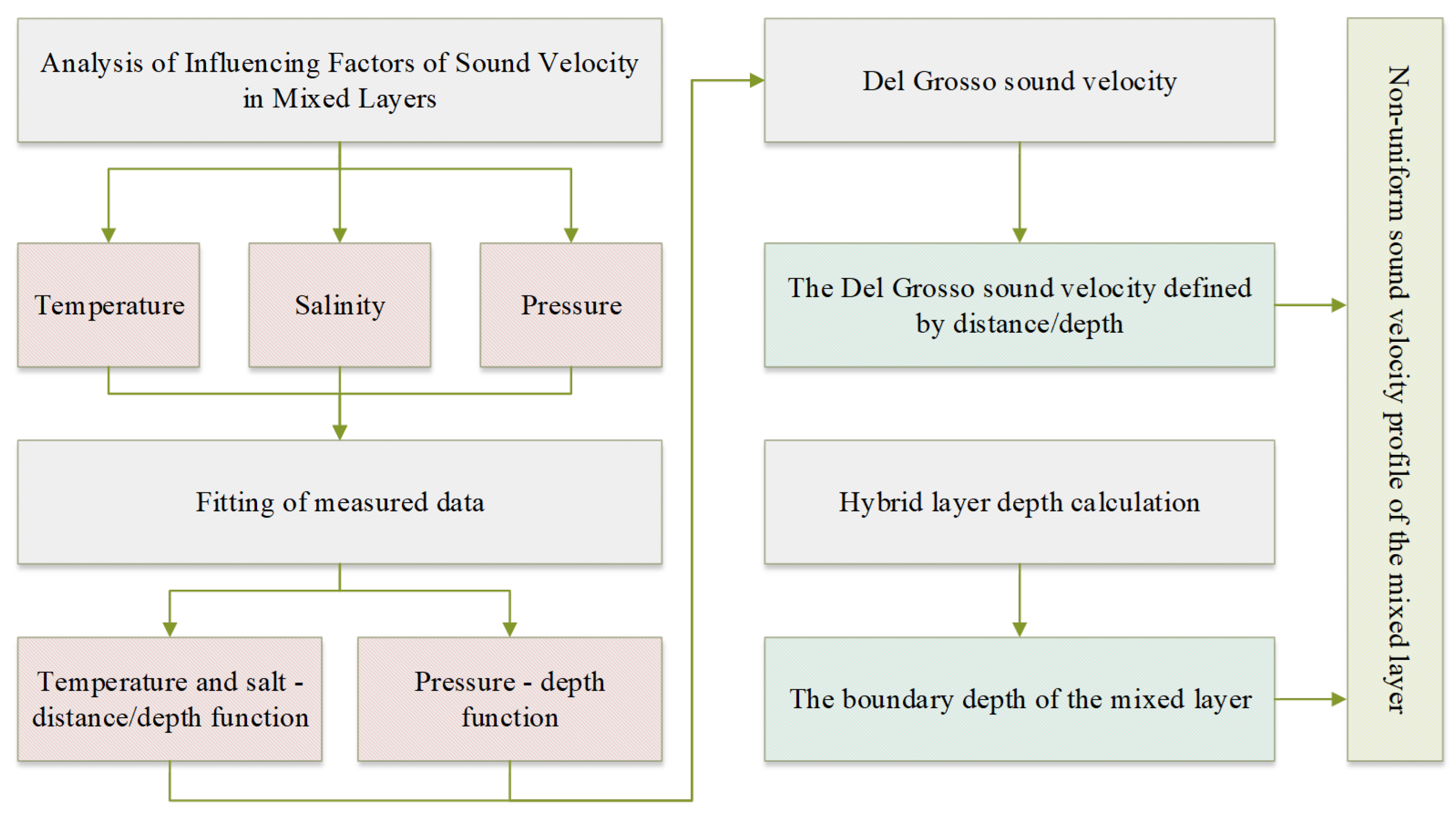
Figure 2.
BOA_Argo data.
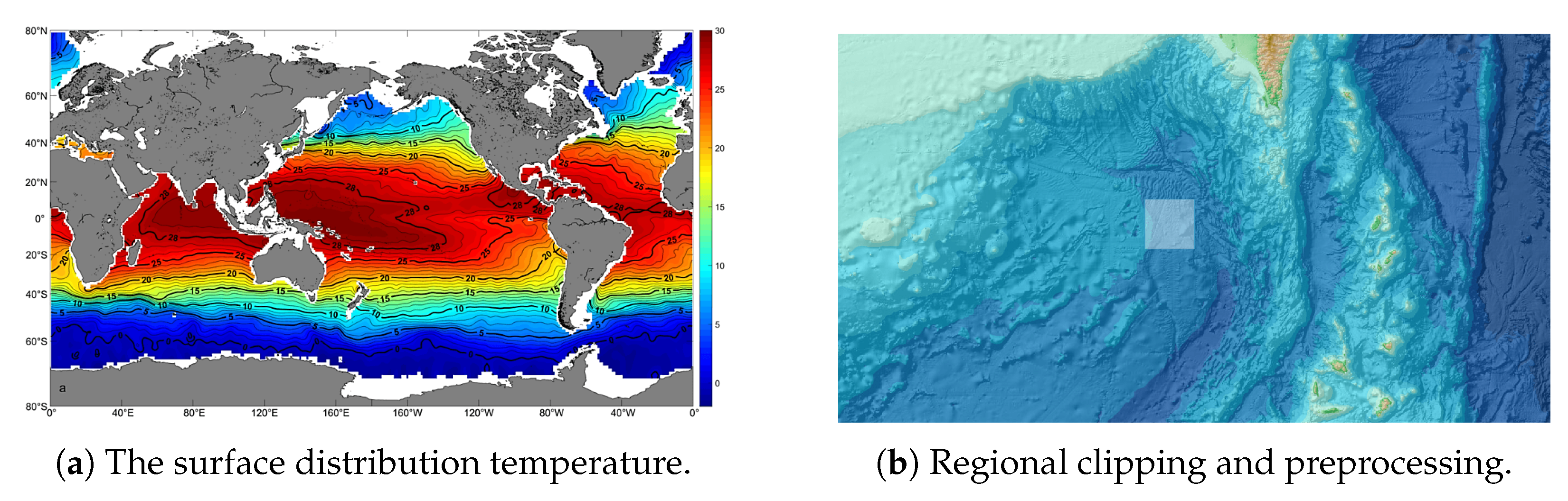
Figure 3.
Comparison of the continuous temperature and salinity distribution model after EOF decomposition with the original data.
Figure 3.
Comparison of the continuous temperature and salinity distribution model after EOF decomposition with the original data.
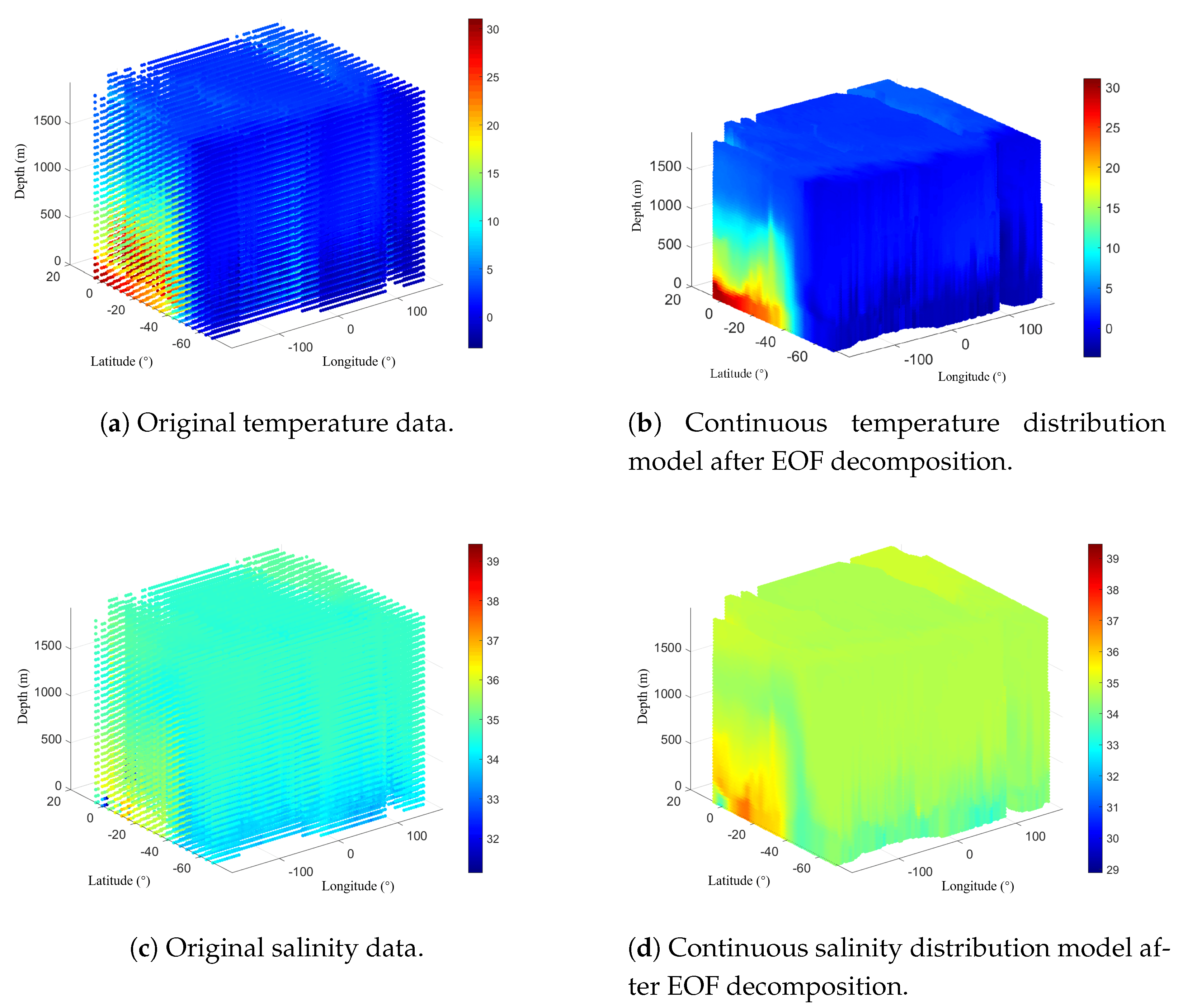
Figure 4.
Schematic of non-uniform sound speed distribution in the mixed layer.
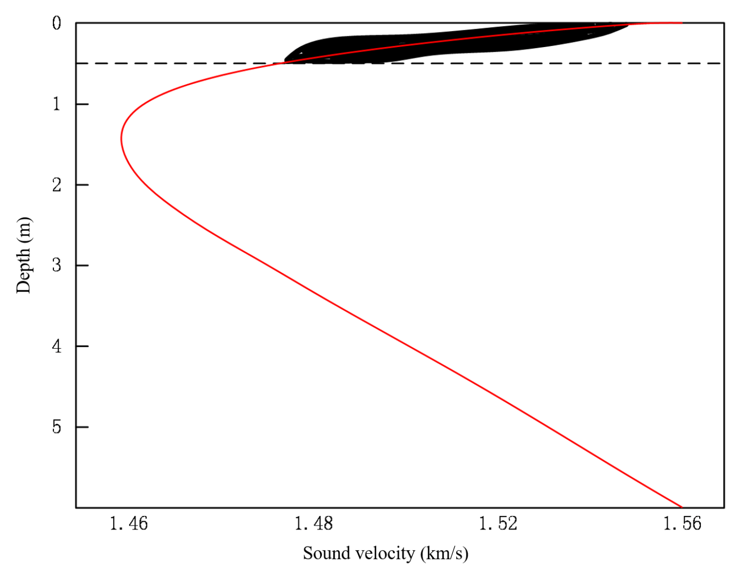
Figure 5.
Horizontal non-uniformity improved ray model path offset.
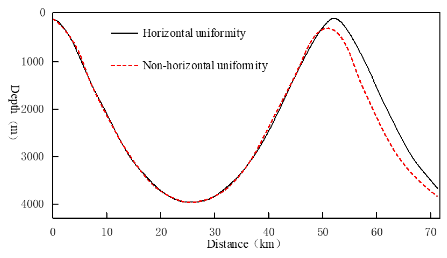
Figure 6.
Convergence Zone Characteristic Parameter Forecast.
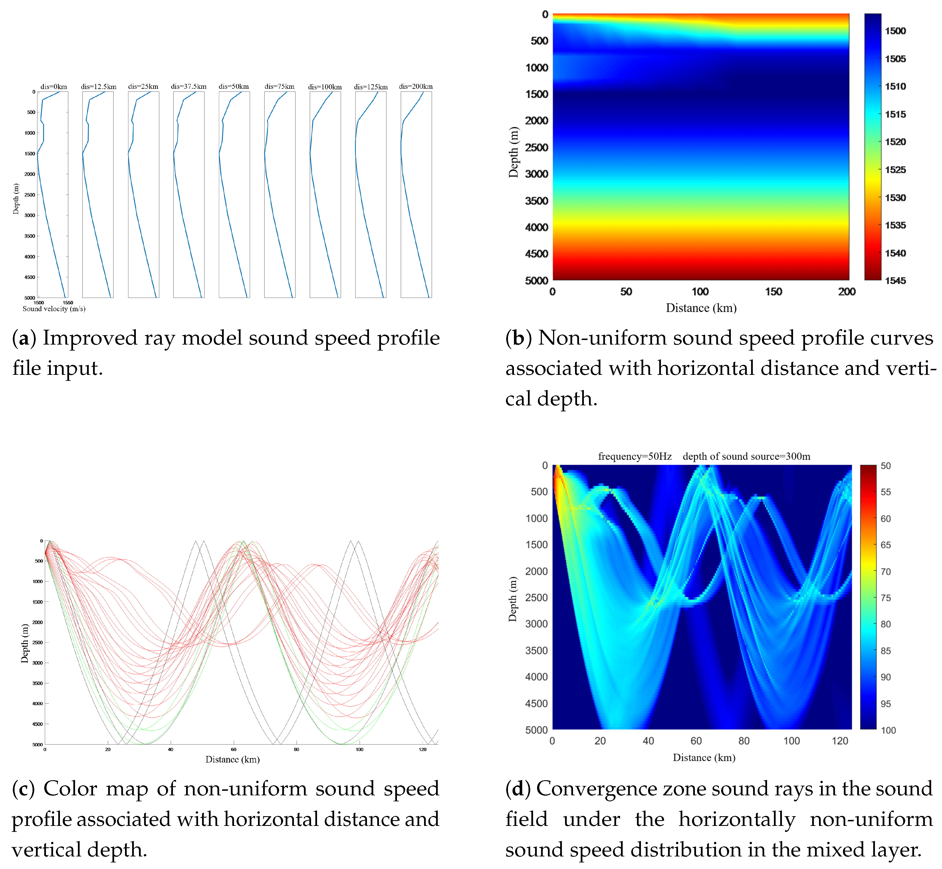
Figure 7.
Typical ocean profile.
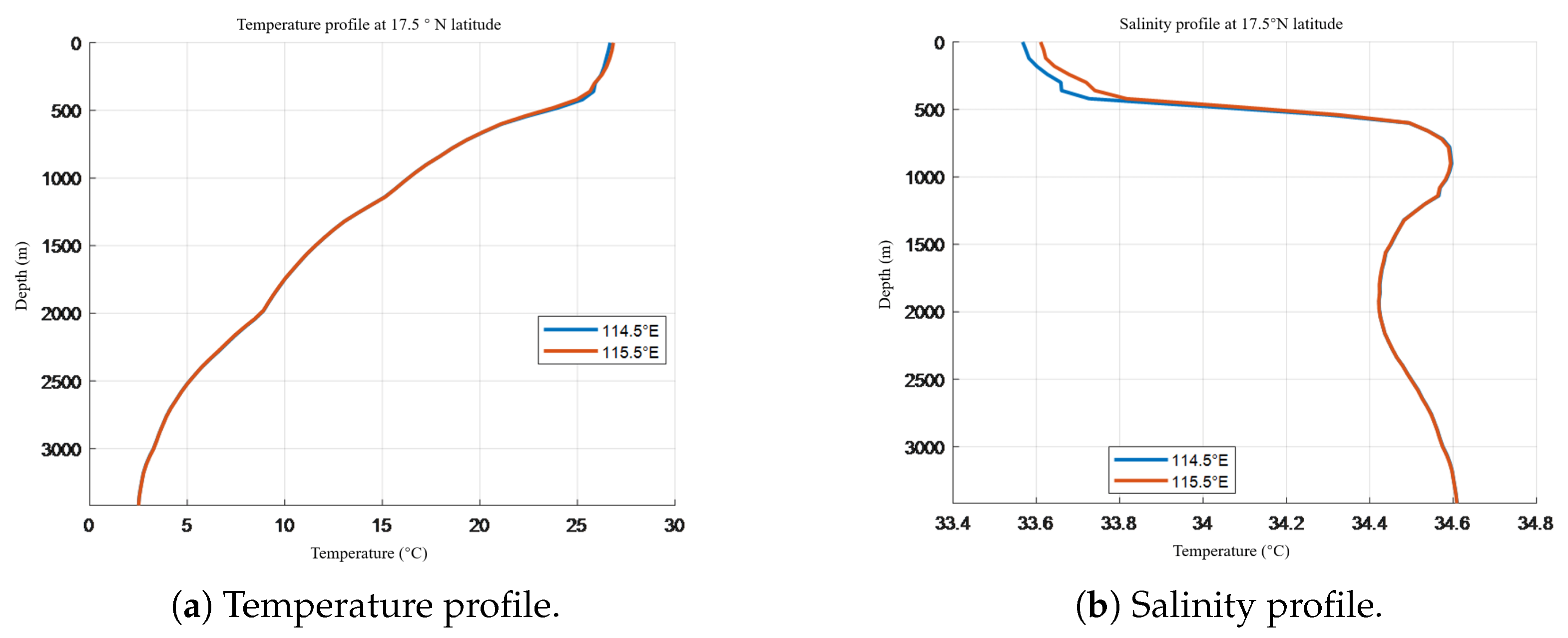
Figure 8.
Horizontally non-uniform sound speed profile curve.
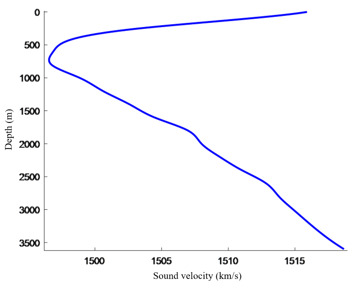
Figure 9.
Simple equivalent sound speed profile of the Bellhop ray model.
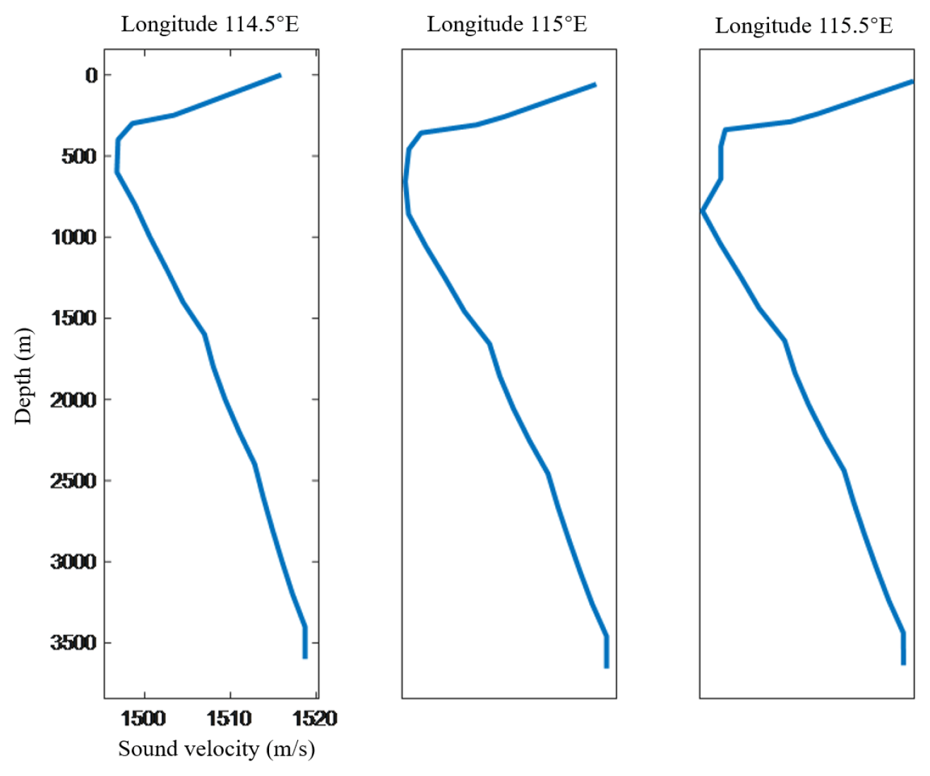
Figure 10.
Color map of horizontally inhomogeneous sound speed profile.
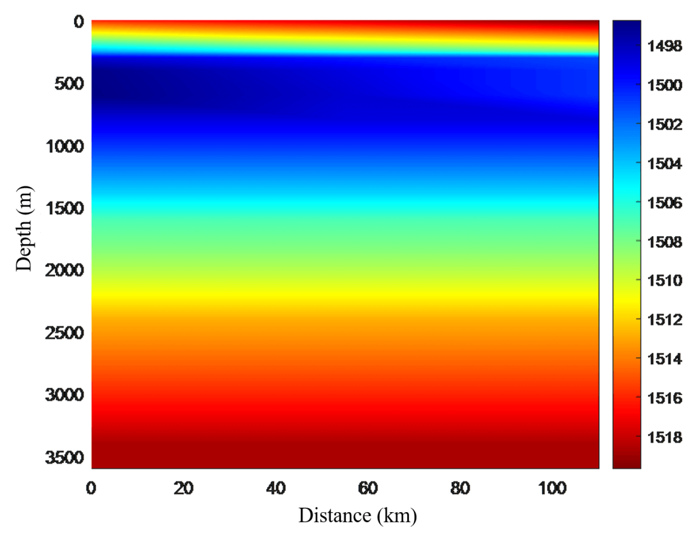
Figure 11.
Comparison of acoustic ray propagation paths.
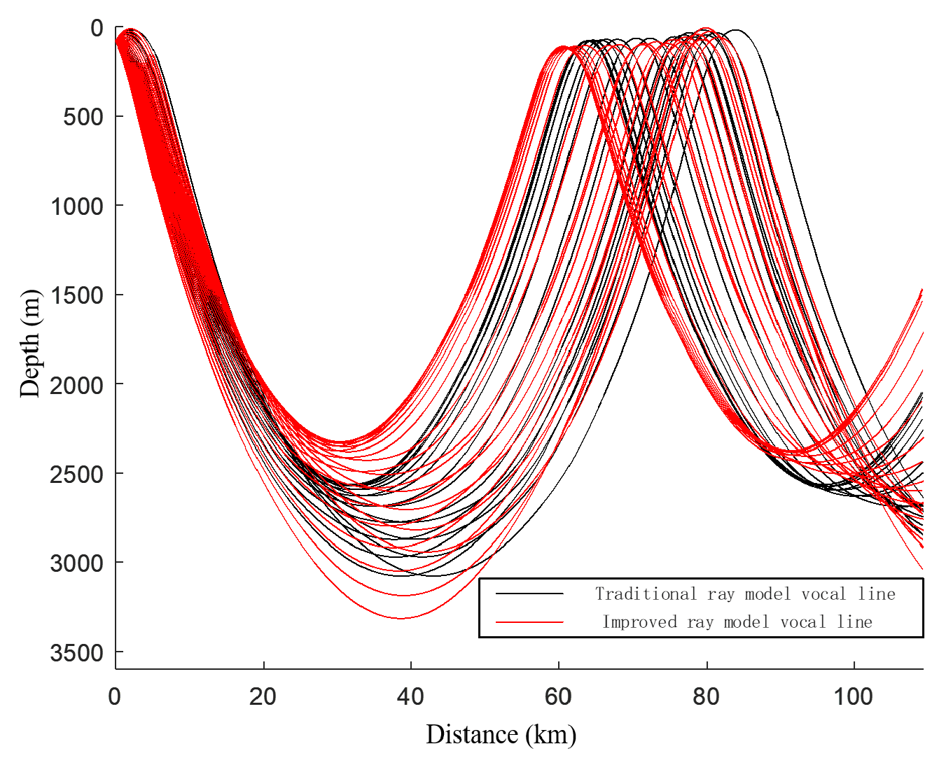
Figure 12.
Comparison of acoustic field parameters in the convergence zone.
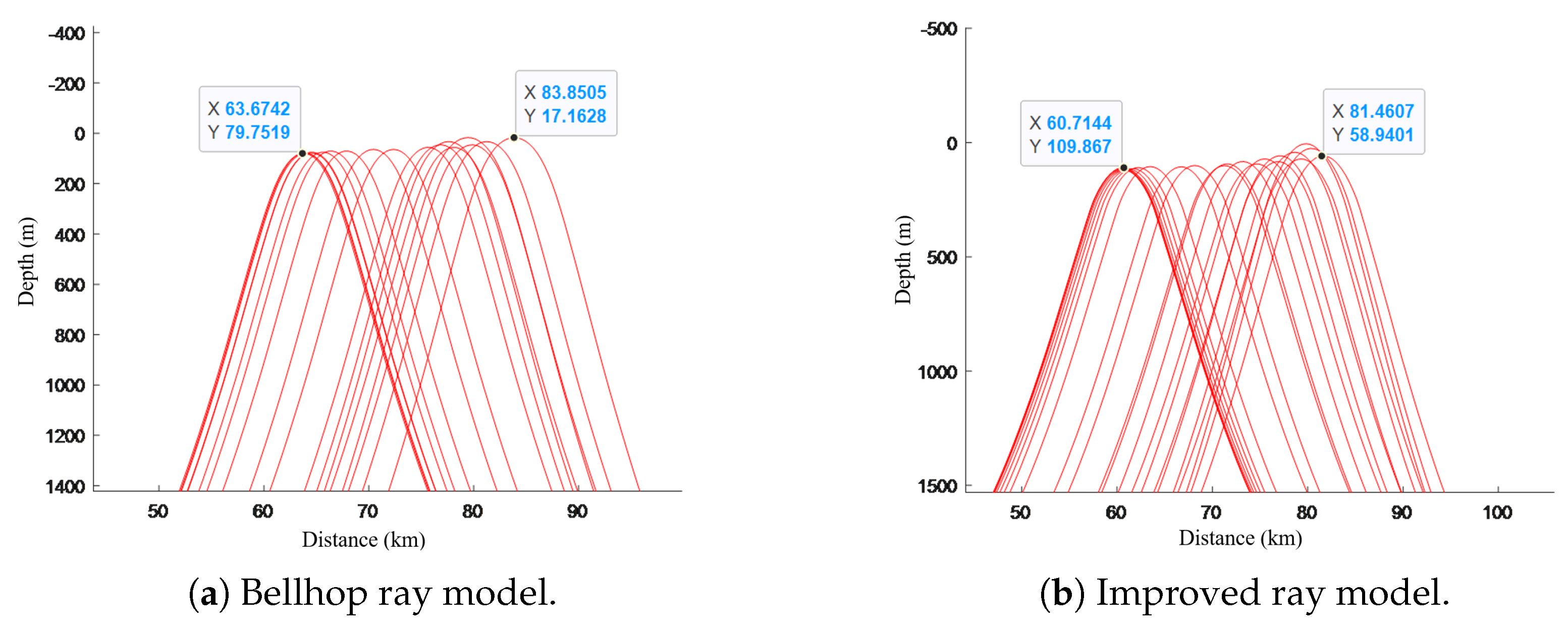
Figure 13.
Acoustic propagation loss comparison.
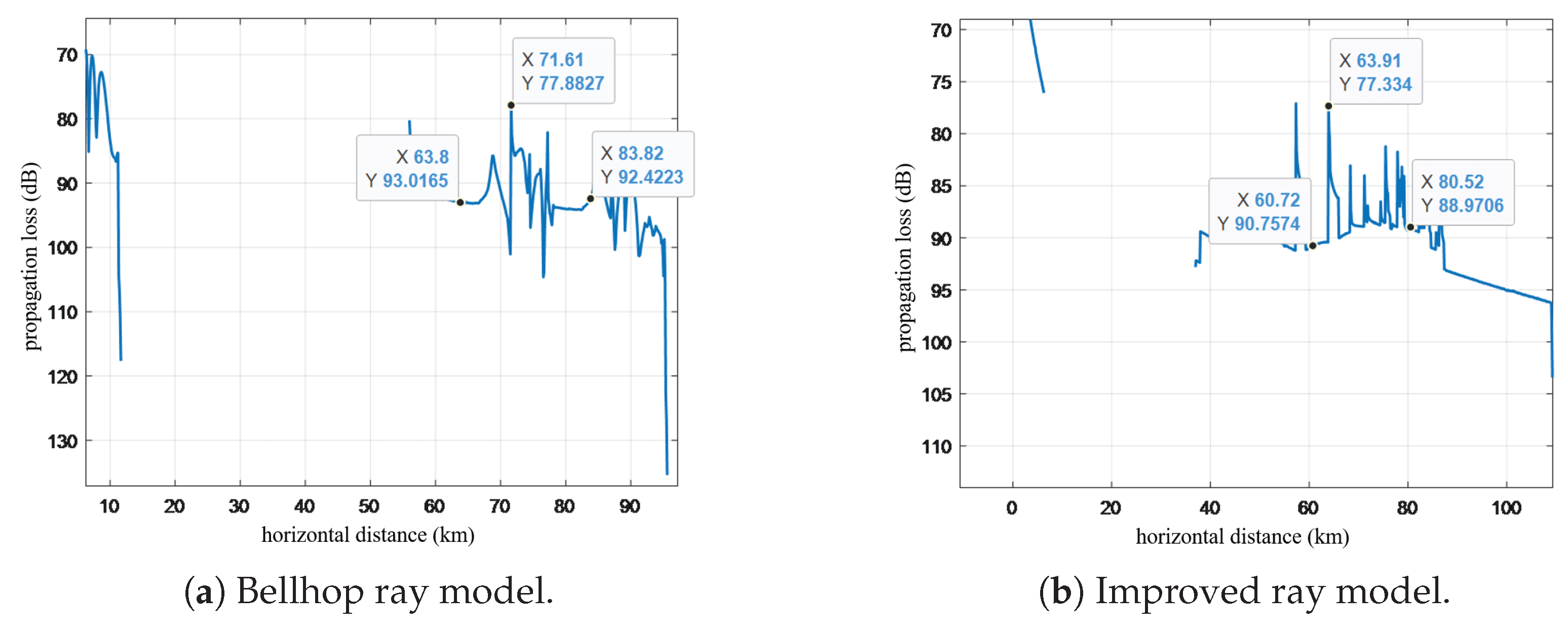

Table 1.
The characteristic parameters of the convergence zone predicted in the South China Sea experiment
Table 1.
The characteristic parameters of the convergence zone predicted in the South China Sea experiment
| Distance(km) | Width(km | Gain(dB) |
| 61.5 | 21.4 | 13.5 |
Table 2.
Comparison of Forecast Results
| Method | Distance(km) | Width (km) | Gain(dB) |
| Measured | 61.5 | 21.4 | 13.5 |
| Bellhop | 63.6742 | 20.1763 | 15.12 |
| Improved | 60.7144 | 20.7463 | 12.67 |
Disclaimer/Publisher’s Note: The statements, opinions and data contained in all publications are solely those of the individual author(s) and contributor(s) and not of MDPI and/or the editor(s). MDPI and/or the editor(s) disclaim responsibility for any injury to people or property resulting from any ideas, methods, instructions or products referred to in the content. |
© 2025 by the authors. Licensee MDPI, Basel, Switzerland. This article is an open access article distributed under the terms and conditions of the Creative Commons Attribution (CC BY) license (http://creativecommons.org/licenses/by/4.0/).
Copyright: This open access article is published under a Creative Commons CC BY 4.0 license, which permit the free download, distribution, and reuse, provided that the author and preprint are cited in any reuse.


