Submitted:
27 April 2025
Posted:
29 April 2025
You are already at the latest version
Abstract
This study examines the combined effects of mesoscale eddies and rough sea surfaces on acoustic propagation in the eastern Arabian Sea and Gulf of Aden during summer mon-soon conditions. Using three-dimensional sound speed fields from CMEMS, sea surface spectra from the SWAN wave model validated by Jason-3 altimetry, and the BELLHOP ray-tracing model, we quantify their synergistic impacts on underwater sound. A Monte Carlo-based dynamic sea surface roughness model is coupled with BELLHOP to analyze multiphysical interactions. Results show that sea surface roughness dominates surface duct propagation, increasing transmission loss by ~20 dB compared to smooth surfaces, while mesoscale eddies deepen the surface duct and broaden convergence zones by up to 5 km. In deeper waters, eddies shift convergence zones and reduce peak sound intensity in the deep sound channel. These findings enhance sonar performance and underwater communication in dynamic, monsoon-influenced marine environments.
Keywords:
numerical simulation
; mesoscale eddies
; rough sea surfaces
; acoustic propagation
; multiphysics coupling
1. Introduction
Underwater acoustic propagation research essentially involves solving wave equations in heterogeneous marine media, with its core focus on revealing how spatiotemporal variations of environmental parameters modulate acoustic fields[1]. Mesoscale processes including eddies, oceanic fronts, and internal waves alter sound speed profile structures through thermohaline redistribution [2,3], leading to acoustic path refraction and modal energy redistribution [4]. Baroclinic instability-generated mesoscale eddies induce potential vorticity anomalies that deform isopycnal surfaces, modifying vertical sound speed gradients. Such perturbations affect convergence zone distributions within the theoretical framework of waveguide invariants [5,6]. Studies have shown that the presence of mesoscale eddies significantly alters the primary characteristics of the acoustic field compared to fields without eddies. These changes include the shift of convergence zones, changes in the order of multipath arrivals, and horizontal refraction issues [7]. Additionally, mesoscale eddies can lead to modifications in the structural characteristics of convergence zones and the emergence or disappearance of surface duct effects[8]. Research on theoretical models for acoustic field calculation under rough sea surfaces has led to the development of many mature theories and methods. Commonly used approaches include the Kirchhoff approximation, the small-slope approximation [9,10], and the RAM (Range-dependent Acoustic Model) based on parabolic equations [11,12]. Scholars have conducted extensive research on the characteristics of acoustic fields under rough sea surfaces, primarily focusing on the effects of acoustic attenuation, spatiotemporal correlations, and the time-of-arrival of signals.
In the Gulf of Aden, acoustic propagation characteristics are controlled by monsoon-driven multiscale processes. The summer southwest monsoon (June-September mean wind speed >12 m/s) activates the Somali Current (surface velocity >1.5 m/s) [13], generating the Great Whirl eddy through barotropic instability. Argo float observations indicate that this eddy modifies thermohaline structures via vertical mixing, producing mixed layer depth anomalies up to 26.7 m in its core region [1]. Enhanced sea surface roughness under monsoon conditions (significant wave height reaching 4 m [14]) creates coupled perturbations through air-sea interactions, establishing compound modulation sources for acoustic propagation [15].
The coupled effects of mesoscale eddies and sea surface roughness on acoustic propagation have gained increasing attention [16,17]. Early theoretical models quantified eddy-induced sound speed variations using quasi-geostrophic potential vorticity equations [5], while contemporary studies employ three-dimensional ocean-acoustic coupled frameworks. Regarding the influence of eddies on sound propagation, [18] utilized the FOR3D model to investigate the impact of a cold eddy in the Luzon Strait on the convergence zone of the sound field based on the 3-D temperature and salinity fields output from the HYCOM model .[19] demonstrated through MITgcm-BELLHOP integration that interactions between Luzon cold eddies and tidal currents shift convergence zones forward by 5 km with 0.1-s arrival delays. Regarding rough surface impacts, [20] compared the acoustic pressure fields generated by broadband sound sources under different wind speed conditions and concluded that sea surface roughness is the primary factor causing acoustic signal attenuation, while bubble scattering and Doppler shifts are secondary factors. [21]applied Ramsurf modeling with PM spectra and Monte Carlo simulations, revealing 4-6 dB increases in transmission loss under realistic sea states compared to smooth surface conditions.
Current research limitations persist in two aspects:
1) Most eddy-acoustic studies assume idealized smooth surfaces, overlooking coupled effects between vortical flows and wind-driven roughness[22];
2) Traditional PM spectra fail to accurately represent sea states in topographically complex regions like the Gulf of Aden, where monsoon-regulated fetch limitations reduce spectral fidelity.
This study develops a coupled model integrating three-dimensional eddy-resolving sound speed fields and sea surface spectra simulated by SWAN (Simulating WAves Nearshore). Through BELLHOP ray tracing simulations, we quantify the synergistic interaction between mesoscale eddies and sea surface roughness on acoustic propagation, providing theoretical support for optimizing underwater detection systems in monsoon-affected seas.
2. Methodology
To accurately characterize sea surface roughness in the target maritime area, the SWAN wave model was implemented to replace the conventional PM spectrum [23]. This approach was combined with the Monte Carlo method (also termed linear filtering technique) to establish a one-dimensional dynamic sea surface roughness model. The study area exceeds 3000 m in depth, satisfying deep-water waveguide assumptions. Furthermore, BELLHOP's multi-patch configuration efficiently incorporates rough sea surface boundaries, making it the ideal choice for acoustic propagation simulations. By parameterizing the upper boundary conditions, this framework systematically integrates sea surface perturbation effects. At the same time, it ensures computational stability in deep-water scenarios.
2.1. Wave Model
The SWAN (Simulating WAves Nearshore) model, developed at Delft University of Technology, represents a third-generation spectral wave model that has reached operational maturity through decades of refinement. Its theoretical foundation is established through the action balance equation derived from energy conservation principles, incorporating the core features of third-generation wave models while specifically addressing shallow-water hydrodynamic requirements[24]. The governing equations are solved using a fully implicit finite-difference scheme, ensuring unconditional numerical stability that eliminates spatial grid and temporal step constraints. The source terms encompass conventional energy components including wind input, nonlinear wave-wave interactions, whitecap dissipation, and bottom friction, with additional incorporation of depth-induced wave breaking mechanisms to enhance simulation fidelity across coastal-offshore transition zones.[25,26]
The SWAN model solves the spectral action balance equation. While spectral energy density becomes non-conservative in ambient currents due to Doppler-shifting and energy transfer, the wave action N(σ, θ) remains a conserved quantity that advects with the sum of group velocity and ambient current velocity. In a Cartesian coordinate system, the wave action balance equation can be expressed as:
In the governing equation, the first term on the left-hand side (LHS) represents the temporal variation rate of wave action density. The second and third terms denote the propagation of wave action in the x- and y-directions of the geographical space, respectively. The fourth term accounts for the advection of wave action in the σ-space (relative frequency domain) induced by ambient currents and varying water depths. The fifth term describes the refraction-induced redistribution of wave action in the θ-space (directional domain), which arises from depth- and current-driven modifications to wave phase speed. The right-hand side (RHS) S/σ encapsulates the source/sink terms, where S aggregates energy inputs and outputs from Wind energy transfer (Sin); Nonlinear wave-wave interactions(Snl); Bottom friction dissipation(Sbot); Whitecap dissipation(Swc); Depth-induced wave breaking(Sds)
The governing velocity components in the wave action balance equation are defined as:
The propagation velocities in the wave action balance equation encapsulate distinct physical mechanisms governing spectral evolution. In geographical space, and Cy represent the total advection velocities in the x- and y-directions, respectively, combining the wave group velocity components (Cg cos θ and Cg sin θ) with ambient current velocities (U and V) to resolve wave-energy transport under coexisting wave-current dynamics. In spectral space, Cσ quantifies the frequency shifting rate in the relative frequency (σ) domain, driven by temporal variations () and spatial gradients of currents or depths (), which collectively induce Doppler-like spectral compression/expansion. Meanwhile, Cθ governs refraction in the directional (θ) domain, where depth- or current-induced gradients (,) redirect wave energy through phase-speed modifications, with the 1/k term (k: wavenumber) ensuring kinematic consistency with the linear dispersion relation .
2.2. Acoustic Ray Model
Selecting an appropriate sound field model is essential for accurately investigating the principles of sound propagation in the ocean. Such a model must be capable of capturing the complexities of the horizontally varying ocean environment. In the 1980s, Porter and Bucker [27] introduced the Gaussian beam approximation, initially used in geoacoustics, into underwater acoustic computations. The model is available through the Acoustics Toolbox, a widely used software suite for underwater acoustic simulations. This innovation led to the development of the BELLHOP ray model, which calculates the sound field based on a given sound speed profile—an essential factor in underwater acoustic propagation. Notably, it can simulate the sound field in acoustic shadow zones and focal dispersion regions, areas where traditional ray acoustics often fail. Additionally, the model addresses challenges associated with low-frequency sound propagation, further enhancing accuracy in such scenarios. Due to its clear physical interpretation and computational efficiency, the BELLHOP ray model has been widely adopted in range-dependent hydroacoustic propagation studies[28,29,30,31,32,33,34,35].
The BELLHOP model employs the Gaussian beam method as its primary approach. The Gaussian beam method models sound propagation using beams of specific width, characterized by two parameters: curvature and width. The intensity distribution of the sound beam is described by a Gaussian function. This approach represents the sound field generated by the source as the superposition of energy contributions from multiple sound beams.[36]
The Gaussian beam model simplifies the vector equation that describes sound propagation into the ray equation and its accompanying equation:
where c is the sound speed; r(s), z(s) indicate the coordinates of the ray in the column coordinate system; s represents the arc length in the direction of the ray. Here, the auxiliary variables ξ(s), ξ(s) are introduced to write the equation in first-order form. A set of concomitant components p(s) and q(s) are used to describe the curvature and width of the ray, and they form the accompanying equation for ray tracing:
where is the sound speed curvature in the normal direction of the ray path. To derive , first note that the derivative of c in the normal direction can be presented as:
where n = (n(r), n(z)) is the normal of the ray and then the derivative is repeated in the normal direction, yielding:
Combining the auxiliary variables in Eq. (6)-(9), finally yielding:
This curvature formula utilizes only the second-order derivative of the sound speed concerning the coordinate r and z. In order to determine the trajectory of each beam and the accompanying parameters, the above equations should be discretized, initial conditions set, and then recurse. By summing the contribution of each beam, the distribution of the sound field can be obtained.
2.3. One-Dimensional Rough Sea Surface Model
Rough sea surfaces critically influence acoustic fields through repeated interactions in surface ducts, necessitating physically consistent sea surface modeling. Current methodologies are divided into two primary categories. Physics-based approaches employ linear/nonlinear wave theories to solve hydrodynamic equations, achieving high fidelity at the cost of computational complexity. Stochastic spectral methods utilize wave spectrum analysis to derive statistical wave characteristics. The sea surface elevation spectrum, defined as the Fourier transform of sea surface height correlation functions, provides measurable harmonic component distributions across wavenumbers. This capability enables efficient surface reconstruction via the Monte Carlo (linear filtering) method.
The ocean wave spectrum is defined as the Fourier transform of the spatial correlation function of sea surface height fluctuations. It quantitatively characterizes the energy distribution of harmonic wave components across the wavenumber domain. This parameter is experimentally measurable and can be obtained through field measurement techniques to capture wave spectral characteristics in specific marine regions.
Based on measured ocean wave spectra, a Monte Carlo method can be employed to reconstruct randomly rough sea surfaces. The technical workflow comprises three key steps. First, discrete spatial sampling of Gaussian white noise is performed. Second, spectral amplitude modulation is applied in the wavenumber domain. Finally, inverse Fourier transformation generates sea surface elevation profiles that satisfy the prescribed spectral properties.
The methodology offers two principal advantages. First, it ensures statistical consistency between reconstructed surfaces and real marine environments by incorporating empirical spectral constraints. Second, its numerical implementation via fast Fourier transforms (FFT) drastically reduces computational complexity, enabling real-time processing capabilities suitable for engineering applications. As a result, this approach has become a standard for sea surface modeling in both research and engineering applications.
The specific Monte Carlo formulation for 1D stochastic rough sea surface modeling is as follows[37]:
This formulation describes a Monte Carlo-based reconstruction of 1D rough sea surfaces using discrete Fourier transforms. The surface elevation at discrete spatial points (where ) is synthesized through an inverse Fourier series summation , with representing discrete wavenumbers. The complex Fourier coefficients are generated by combining the ocean wave spectrum with Gaussian random phases: , where ϕ follows distinct statistical rules for different wavenumber indices. For non-symmetric modes (), ϕ is constructed using complex normal variables, ensuring Hermitian symmetry in the spatial domain. At symmetric wavenumbers (), real-valued Gaussian variables N(0, 1) are used instead to maintain physical consistency. This dual treatment preserves both the spectral energy distribution (via ) and the stochastic nature of sea surface fluctuations.
3. Data and Model
3.1. Mesoscale Eddy Data
The hydrographic data utilized in this study were sourced from the Copernicus Marine Environment Monitoring Service (CMEMS, https://marine.copernicus.eu/), while the bathymetric data were obtained from the ETOPO2022 dataset (https://www.ncei.noaa.gov/). The temporal and spatial scope of the analysis is confined to 00:00 UTC on July 31, 2024, in the eastern Arabian Sea, adjacent to the Gulf of Aden.
Prior to conducting acoustic propagation simulations, it is imperative to validate the presence of mesoscale eddies within the study area. Following the acquisition of hydrographic data from CMEMS, the Parallel Eddy Tracking (PET) algorithm was employed for eddy identification. The PET algorithm, which integrates closed contour topology and overlapping trajectory optimization techniques[38], serves as the core detection framework for the global mesoscale eddy database META3.1exp[39]. This algorithm reconstructs the three-dimensional kinematic characteristics of eddies based on the Absolute Dynamic Topography (ADT) field, demonstrating an 18% improvement in eddy boundary identification accuracy in regions of strong currents compared to traditional Sea Level Anomaly (SLA) methods. In this study, the PET tool was applied to perform eddy trajectory backtracking in the target region, thereby providing a robust eddy dynamic background field for subsequent acoustic propagation modeling. The results of the eddy identification are presented as (Figure 1):
The study area is located in the eastern Arabian Sea, adjacent to the Gulf of Aden(Figure 2), spanning the region between 5.5°–9.5°N and 52°–56°E. For the analysis, the temperature and salinity fields at 00:00 UTC on July 31, 2024, were selected to calculate the sound speed profile in seawater.
Specifically, nine depth levels (0 m, 50 m, 100 m, 150 m, 200 m, 300 m, 400 m, 600 m, and 800 m) were chosen. These levels were used to display the three-dimensional sound speed structure within the region bounded by 5.5°–9.5°N and 52°–56°E (Figure 3).
The mesoscale eddy structure is evident, with a horizontal scale of up to 400 km. Its core is approximately located at 7.5°N, 54°E, where the sound speed reaches its maximum value. While the eddy's morphology is distinct in the upper 200 m layer, the core shifts and the structure gradually weakens with increasing depth.
To further investigate the characteristics of sound speed near the eddy core, Figure 4 illustrates the sound speed anomalies along the vertical sections at 54°E and 7.5°N. The anomalies induced by the warm eddy extend to a depth of approximately 1000 m. The strongest eddy signature is observed around 200 m below the surface, consistent with Figure 3. At the eddy core, the maximum sound speed anomaly reaches approximately 8 m/s. The corresponding latitude and longitude provide precise horizontal coordinates for the eddy core.
3.2. SWAN Model Setup
Given the complex seabed topography and significant coastline effects in the eastern Gulf of Aden, this study employs the third-generation wave model SWAN (Simulating WAves Nearshore) to conduct high-precision wave numerical simulations. The SWAN model solves the wave action balance equation (WABE), incorporating physical processes such as wave generation, nonlinear wave-wave interactions, whitecapping dissipation, and bottom friction dissipation, making it particularly suitable for simulating wave evolution in nearshore regions with complex topography.
The study area focuses on the eastern Arabian Sea and Gulf of Aden (48-55°E, 5-11°N). An unstructured triangular mesh is utilized for spatial discretization, comprising 28,093 nodes with an average grid resolution of 3 km. Grid refinement is implemented in regions with prominent mesoscale eddies. The simulation period spans from 00:00 UTC on July 27, 2024, to 00:00 UTC on July 31, 2024 (a total of 97 hours), covering a typical summer mesoscale eddy activity period. To verify the correctness of the model, add the model from 00:00 UTC on July 17, 2024, to 00:00 on July 21, 2024, for simulation calculations.
In this study, 55 equally spaced sampling points were deployed along the 54°E meridian (7.5°N–10°N) within the SWAN model, with a spacing of 5 km and a total span of approximately 275 km (Figure 5). This deployment was designed to capture the spatial variability of wave spectra across the study area.
One-dimensional wave spectrum data from the last hour of the simulation was extracted and, based on the Monte Carlo method, transformed into one-dimensional static sea surface realizations using the wave spectrum parameters output by SWAN. With each sampling point simulating a 5 km rough sea surface, the total simulation length reached 275 km. Figure 6 presents an example of the simulated rough sea surface.
To validate whether the wave spectra provided by SWAN can better simulate rough sea surfaces, and considering the stochastic nature of the Monte Carlo method in generating rough sea surfaces, it is challenging to determine which method is superior based solely on the simulated rough sea surfaces. Therefore, the wave energy density spectra calculated by SWAN were used to derive significant wave height (SWH) using Equation (12)-(13). Furthermore, the classical PM spectrum, combined with wind field data, was utilized to calculate the SWH for PM-based sea surface simulations using Equation (14)-(16).
To validate model reliability, a comparative analysis was conducted between Jason-3 satellite Ku-band SWH data (https://www.ncei.noaa.gov/data/oceans/) and SWAN-modeled SWH. The comparison revealed excellent agreement between the SWAN-derived SWH and Jason-3 observations. Furthermore, SWH calculations based on the ERA5 wind field-derived PM spectrum were compared with both Jason-3 measurements and SWAN simulations(Figure 7). This methodological enhancement improved the traditional SWH calculation methodology, demonstrating that the SWAN model more accurately represents real marine conditions compared to conventional approaches.
In Figure 7, red represents Jason-3 altimetry data, green denotes SWH calculated using the ERA5 wind fields with the PM spectrum, and blue corresponds to SWAN-modeled results. Comparison with data from July 18-19 demonstrates that the SWAN-derived SWH achieves a mean RMSE of 0.17, whereas the PM spectrum-based calculation yields a higher mean RMSE of 0.40. Similarly, for the July 28-29 period, the SWAN results show a mean RMSE of 0.20, compared to the PM spectrum's mean RMSE of 0.42. These results indicate that traditional PM spectrum-based SWH calculations systematically overestimate wave heights, likely due to the PM spectrum's exclusive consideration of fully-developed sea states. In contrast, the SWAN model outputs align more closely with observational altimetry data, providing reliable foundations for subsequent rough sea surface modeling.
4. Sound Propagation
This study employs the BELLHOP acoustic model to systematically analyze the mechanisms of acoustic propagation variability under the multiphysical coupling of mesoscale eddies and rough sea surfaces, aiming to understand their combined effects on underwater sound propagation. The experimental region is centered at the core of a mesoscale eddy (7.5°N, 54°E). A circular computational domain with a radius of 200 km is constructed around it (Figure 2a).
The seafloor topography in this region is flat, with a water depth of approximately 5303 m. This effectively reduces the impact of topographic scattering on acoustic propagation. Detailed parameter settings for the model are provided in Table 1.
In this study, the 54°E meridian (dashed line in Figure 2b) is selected as the cross-section for analyzing acoustic propagation characteristics due to its alignment with the mesoscale eddy core. A three-layer sound source deployment scheme is implemented to investigate the response mechanisms at different depths: 10 m depth to represent surface duct propagation, 200 m depth to examine the formation mechanisms of convergence zones, and 800 m depth to analyze the propagation patterns of the deep sound channel [40].
The experimental design includes four comparative scenarios (Table 2):
1.Baseline scenario: A static sea surface and homogeneous water body.
2.Pure eddy scenario: Retains only the mesoscale eddy's temperature and salinity structures.
3.Pure roughness scenario: Combines a wind-wave field described by the PM spectrum with a flat-bottom topography.
4.Fully coupled scenario: Joint effects of mesoscale eddies and rough sea surfaces.
Using stratified comparisons, this study quantitatively examines three mechanisms:
1.How mesoscale eddy-induced sound speed anomalies affect the reconstruction of convergence zones.
2.How rough sea surfaces influence near-field scattering losses.
3.The nonlinear coupling effects of multi-scale marine environmental factors.
4.1. Experiment 1: Baseline Scenario
The first sub-experiment serves as the baseline scenario for comparative analysis with the other three cases, providing a reference to isolate the effects of mesoscale eddies and sea surface roughness on acoustic propagation. This sub-experiment excludes the influence of mesoscale eddies and sea surface roughness on acoustic propagation. The temperature and salinity data from point A (55.5°E, 9°N) in Figure 2b is used as representative values for the experimental region. Additionally, the sea surface is set to a flat, calm condition to eliminate roughness effects. These conditions are then implemented in the BELLHOP model to simulate acoustic propagation in a simplified environment. A comparison of sound speed profiles between point A and the eddy center is presented in Figure 8.
Figure 9 illustrates the transmission loss for three distinct acoustic propagation modes—surface duct propagation, convergence zone propagation, and deep sound channel propagation—along the northward direction (red dashed line) from the sound source in Figure 2b.
When the sound source is placed at a depth of 10 m, a distinct surface duct is observed, characterized by low transmission loss due to the trapping of sound energy near the sea surface. With the sound source positioned at 200 m depth, three convergence zones appear within the 200 km propagation range, reflecting the focusing of sound energy at specific intervals due to the interaction with the mesoscale eddy's sound speed structure. When the sound source is set at 800 m depth, four convergence zones emerge within the same propagation range, demonstrating the influence of the deep sound channel on long-range acoustic propagation.
As shown in Figure 9, the sound rays are distributed throughout the propagation region, closely interacting with the sea surface and the mesoscale eddy's thermohaline structure. These interactions highlight the complex modulation effects of the marine environment on acoustic propagation, providing a foundation for subsequent analysis of multiphysical coupling mechanisms.
4.2. Experiment 2: Pure Eddy Scenario
In this sub-experiment, the impact of mesoscale eddies on the sound speed field is exclusively investigated. The distribution of sound speed anomalies in the vertical cross-section corresponds to the spatial pattern shown in Figure 8. To more intuitively observe the variation of acoustic transmission loss with propagation distance, one-dimensional transmission loss curves are provided for each sound source depth (Figure 10). These curves highlight the modulation effects of mesoscale eddy-induced sound speed anomalies on acoustic propagation, providing insights into the interaction between ocean dynamics and underwater acoustics. Sz denotes the source depth, and Rz denotes the receiver depth.
Figure 10a compares the transmission loss characteristics under the influence of a mesoscale eddy with those in the baseline environment. When both the sound source and receiver are positioned at a depth of 10 m, the transmission loss curve exhibits periodic fluctuations (red curve) due to perturbations in the sound speed profile caused by the warm eddy. The fluctuation amplitude increases by approximately 5 dB compared to the baseline environment (black curve). This oscillatory behavior arises from the phase interference of sound wave propagation paths altered by the sound speed anomaly induced by the mesoscale eddy. Notably, when the propagation distance exceeds 150 km, the transmission loss under eddy influence decreases by about 3-5 dB compared to the baseline, suggesting a potential waveguide enhancement effect at this distance scale.
When the sound source and receiver are both at a depth of 200 m, the first, second, and third convergence zones shift forward by 4 km, 10 km, and 17 km, respectively, under the influence of the mesoscale eddy. The peak energy in the first and second convergence zones decreases by approximately 6 dB compared to the baseline. However, in non-convergence regions, the transmission loss under eddy influence is slightly lower than that in the baseline scenario. To investigate this phenomenon, the sound ray diagram is plotted in Figure 11. Compared to the baseline, the sound speed gradient under the warm eddy is steeper, resulting in a smaller curvature radius of the limiting rays. This causes the convergence positions to shift forward and the turning depth to increase, reducing the number of red rays that retain most of the acoustic energy. Consequently, the transmission loss in the convergence zones increases. Some rays, after reflecting without touching the seafloor, reverse again and reach the sea surface, leaking into the shadow zone. This leads to slightly lower transmission loss in the shadow zone compared to the baseline scenario.
When both the sound source and receiver are positioned at a depth of 800 m, the convergence zones still exhibit a forward shift under the influence of the mesoscale eddy. Additionally, the number of convergence zones increases, while their characteristic features become less pronounced. This phenomenon can be attributed to the same mechanisms described earlier, where the altered sound speed gradient and reduced curvature radius of the limiting rays lead to changes in the convergence patterns and energy distribution. These observations highlight the complex interplay between mesoscale eddies and deep-sea acoustic propagation, particularly in the context of the deep sound channel.
4.3. Experiment 3: Pure Rough Sea Surface Scenario
In this experiment, the hydrological environment is maintained consistent with the baseline scenario to ensure an identical sound speed field, focusing solely on analyzing the impact of rough sea surfaces on acoustic propagation. A schematic of the rough sea surface (part) is illustrated in Figure 6. In the BELLHOP model, the sea surface height is updated every 0.25 km. The simulation results for Experiment 1 (baseline) and Experiment 3 (rough sea surface) are presented in Figure 12.
Figure 12a shows the transmission loss when the sound source is at a depth of 10 m, without considering eddies or rough sea surfaces. Figure 12b depicts the transmission loss when only the influence of rough sea surfaces is considered. To more intuitively observe the variation of acoustic transmission loss with distance, one-dimensional transmission loss curves for the 10 m sound source depth are provided in Figure 13.
When sound waves interact with the sea surface, they follow Snell's law of refraction. Within the surface duct, the sound rays undergo continuous refraction due to the sound speed gradient, effectively confining energy within the duct and leading to significant energy accumulation in convergence zones. However, when the sea surface is rough, the interaction between sound waves and the irregular surface alters the incident angles of the rays. According to Snell's law, minor changes in the incident angle result in significant adjustments to the refraction angle. Consequently, some rays escape the surface duct due to increased refraction angles, highlighting the modulation effects of sea surface roughness on acoustic propagation.
Assuming the ray's launch angle is , the sound speed at the source location is , and the ray's turning angle at the lower boundary of the surface duct is =0° with the sound speed at the lower boundary being , Snell's law of refraction = yields = , which defines the critical angle at which the ray turns. Therefore, rays with launch angles within interact only with the sea surface and propagate within the surface duct. As the grazing angle increases, the rays no longer turn upward but instead turn downward, becoming rays that no longer interact with the sea surface. When the grazing angle continues to increase, the rays escape the surface duct and follow the convergence zone propagation pattern.
This process reduces the energy density within the surface duct and weakens the sound intensity distribution in the far-field convergence zones. The 'escaped' rays enhance the convergence zone characteristics, resulting in nearly identical peak energy levels as in Experiment 1. However, in the shadow zone, the energy difference caused by the rough sea surface is approximately 20 dB. These findings underscore the significant impact of sea surface roughness on acoustic propagation, particularly in altering energy distribution between the surface duct, convergence zones, and shadow zones.
When the sound source is positioned at depths of 200 m and 800 m, and only the influence of rough sea surfaces is considered, the relationship between distance and propagation loss is illustrated in Figure 14. The results show good agreement in both scenarios, indicating that the impact of rough sea surfaces on convergence zone propagation and deep sound channel propagation is relatively minor. This suggests that the primary effects of sea surface roughness are confined to near-surface acoustic propagation, while deeper propagation modes remain largely unaffected.
4.4. Experiment 4: Coupled Rough Sea Surface and Eddy Scenario
In this experiment, the sound speed field is derived from CMEMS hydrological data combined with empirical formulas, while the upper boundary for acoustic propagation is obtained using the SWAN wave model to generate the wave spectrum of the target area, combined with the Monte Carlo method, representing a realistic and complex marine environment. Acoustic propagation analysis is conducted using the sound speed field and rough sea surface conditions at 00:00 on July 31. For comparative analysis, transmission loss curves at different depths are provided (Figure 15). The black curve represents Experiment 1 (baseline), the red curve represents Experiment 2 (pure eddy), the blue curve represents Experiment 3 (pure rough sea surface), and the green curve represents Experiment 4 (coupled rough sea surface and eddy).
As shown in the figures, when the sound source is positioned at a depth of 10 m, the acoustic energy is primarily confined within the surface duct. The propagation loss is mainly influenced by the rough sea surface, while the presence of the eddy slightly reduces the propagation loss and weakens the convergence zone characteristics. This is likely because the eddy expands the depth of the surface duct, reducing the escape of sound rays and thereby increasing the acoustic energy compared to the scenario with only rough sea surfaces.
When the sound source is set at depths of 200 m and 800 m, the blue and black curves show good agreement, indicating that the rough sea surface has a minimal impact on acoustic propagation at these depths. The presence of the eddy causes the convergence zones to shift forward and reduces their peak energy, consistent with the findings in Experiment 2. When both rough sea surfaces and eddies are considered, the green and red curves exhibit good agreement, suggesting that the eddy dominates the propagation loss. Additionally, the rough sea surface stabilizes the acoustic energy, reducing fluctuations in propagation loss.
The conclusions drawn from these three scenarios are relatively general and do not clearly distinguish the boundary depth at which rough sea surfaces or eddies play a dominant role. Therefore, a supplementary experiment is designed. Considering that the influence of rough sea surfaces is closely related to the surface duct, Figure 8 shows that the sound speed in Experiment 1 exhibits a positive gradient above 40 m and a negative gradient below 40 m. Under eddy influence, the sound speed profile maintains a positive gradient up to 80 m. Thus, the sound source in the supplementary experiment is set at a depth of 40 m. In Experiment 1, the sound rays follow the convergence zone propagation pattern, while in Experiment 2, they still adhere to the surface duct propagation rules. The resulting one-dimensional propagation loss plot is shown in Figure 16.
In Experiment 1 (baseline), represented by the black curve, the sound rays are not confined to the surface duct, resulting in distinct convergence zones and shadow zones.
In Experiment 2 (pure eddy), represented by the red curve, the higher sea surface temperature expands the range of the surface duct, confining most of the acoustic energy within it. As a result, the sound ray fluctuations are relatively smooth, with a gradual decrease in propagation loss over distance. Compared to the baseline, the propagation loss shows significant differences.
In Experiment 3 (pure rough sea surface), represented by the blue curve, prominent convergence zones and shadow zones still exist. However, the convergence zones shift forward by approximately 5 km compared to Experiment 1, while the peak energy remains unchanged. This phenomenon may be related to the excessive refraction of sound rays caused by the rough sea surface. It indicates that rough sea surfaces not only affect the propagation mechanisms within the surface duct but also influence sound rays in shallow water that follow the convergence zone propagation pattern.
When both rough sea surfaces and eddies are considered (Experiment 4), represented by the green curve, the overall acoustic energy increases compared to Experiment 3, and the convergence zone characteristics are weakened. This is consistent with the earlier explanation that the warm eddy expands the surface duct, concentrating the acoustic energy. The significant difference between the red and green curves is due to the destruction of the surface duct by the rough sea surface, causing sound rays to 'escape' and reducing the energy in the green curve. Compared to the black curve, the blue curve shows a partial forward shift, indicating that when the sound source is in shallow water and follows the convergence zone propagation pattern, rough sea surfaces still have an impact, albeit much smaller than their effect on the surface duct.
5. Conclusions
This study systematically reveals the synergistic regulation mechanism of mesoscale eddies and rough sea surfaces on acoustic propagation in the Gulf of Aden during summer by constructing a SWAN-BELLHOP multiphysics coupling model, validated against Jason-3 satellite altimetry data to ensure the accuracy of the SWAN simulations. Key findings demonstrate that rough sea surfaces dominate near-field propagation loss in the surface duct (10 m depth), increasing it by approximately 20 dB compared to an ideal smooth sea surface, while mesoscale eddies expand the surface duct depth from 40 m to 80 m, reducing acoustic energy leakage and modulating convergence zone characteristics. At the transition depth (40 m), rough sea surfaces cause the first convergence zone to shift forward by approximately 5 km, with unchanged peak sound intensity, whereas mesoscale eddies enhance the trapping efficiency of the surface duct, re-confining escaped sound rays and providing insights for optimizing shallow-water sonar performance. In deep-water propagation (≥200 m), mesoscale eddies dominate, with warm eddies (Δc = 8.3 m/s) shifting convergence zones forward and attenuating peak sound intensity by approximately 10 dB, while rough sea surfaces exhibit negligible influence. The established multiscale coupling model of mesoscale eddies-rough sea surfaces-acoustic analysis' overcomes the limitations of traditional single-factor methods, improving the reliability of acoustic propagation predictions under complex sea conditions by introducing SWAN-simulated wave spectra to replace the classical PM spectrum. These findings provide critical theoretical support for underwater target detection and acoustic communication system optimization in the Gulf of Aden, with direct applications in sonar array deployment depth selection and dynamic convergence zone correction.
6. Patents
Author Contributions
Conceptualization, S.J.; methodology, C.X.; validation, Z.S.; investigation, Z.S.; writing—original draft preparation, Z.S. All authors have read and agreed to the published version of the manuscript.
Funding
This research was funded by the National Natural Science Foundation of China (Grant No. 12201636); Research Fund of National University of Defense Technology (Grant No. ZK22-37); Science and Technology Innovation Program of Hunan Province (Grant No. 2023RC3013); Hunan Provincial Natural Science Fund for Excellent Youths (Grant No. 2023JJ20046); and Young Elite Scientists Sponsorship Program by China Association for Science and Technology (Grant No. 2023-JCJQ-QT-049).
Conflicts of Interest
The authors declare no conflicts of interest.
Abbreviations
The following abbreviations are used in this manuscript:
| PM | Pierson-Moskowitz Spectrum |
| RHS | Right side hand |
| PET | Parallel Eddy Tracking |
| SWH | significant wave height |
| SOFAR | Sound Fixing and Ranging Channel |
| Sz | Source Depth |
| Rz | Receiver Depth |
References
- Chen, C.; Jin, T.; Zhou, Z. Effect of Eddy on Acoustic Propagation from the Surface Duct Perspective. Applied Acoustics 2019, 150, 190–197. [Google Scholar] [CrossRef]
- Chen, W.; Zhang, Y.; Liu, Y.; Ma, L.; Wang, H.; Ren, K.; Chen, S. Parametric Model for Eddies-Induced Sound Speed Anomaly in Five Active Mesoscale Eddy Regions. Journal of Geophysical Research: Oceans 2022, 127, e2022JC018408. [Google Scholar] [CrossRef]
- Zhou, J.-X.; Zhang, X.-Z.; Peng, Z.; Martin, J.S. Sea Surface Effect on Shallow-Water Reverberation. The Journal of the Acoustical Society of America 2007, 121, 98–107. [Google Scholar] [CrossRef]
- Alpers, W. Monte Carlo Simulations for Studying the Relationship between Ocean Wave and Synthetic Aperture Radar Image Spectra. Journal of Geophysical Research: Oceans 1983, 88, 1745–1759. [Google Scholar] [CrossRef]
- Jian, Y.J.; Zhang, J.; Liu, Q.S.; Wang, Y.F. Effect of Mesoscale Eddies on Underwater Sound Propagation. Applied Acoustics 2009, 70, 432–440. [Google Scholar] [CrossRef]
- R. J. Burkholder; M. R. Pino; F. Obelleiro A Monte Carlo Study of the Rough-Sea-Surface Influence on the Radar Scattering from Two-Dimensional Ships. IEEE Antennas and Propagation Magazine 2001, 43, 25–33. [CrossRef]
- Munk, W.H. Horizontal Deflection of Acoustic Paths by Mesoscale Eddies. Journal of Physical Oceanography 1980, 10, 596–604. [Google Scholar] [CrossRef]
- Zhang; Cheng; Qiu Abnormal Features of the Convergence Zone Caused by the Cold Eddy in Western Pacific. Marine science bulletin 2015, 34, 130–137. [CrossRef]
- Broschat, S.L.; Thorsos, E.I. An Investigation of the Small Slope Approximation for Scattering from Rough Surfaces. Part II. Numerical Studies. The Journal of the Acoustical Society of America 1997, 101, 2615–2625. [Google Scholar] [CrossRef]
- Thorsos, E.I.; Broschat, S.L. An Investigation of the Small Slope Approximation for Scattering from Rough Surfaces. Part I. Theory. The Journal of the Acoustical Society of America 1995, 97, 2082–2093. [Google Scholar] [CrossRef]
- Collins, M.D. Applications and Time-domain Solution of Higher-order Parabolic Equations in Underwater Acoustics. The Journal of the Acoustical Society of America 1989, 86, 1097–1102. [Google Scholar] [CrossRef]
- Coury, R.A.; Siegmann, W.L.; Collins, M.D. Three-dimensional Acoustic Propagation in a Waveguide of Variable Thickness. The Journal of the Acoustical Society of America 1995, 97, 3313–3313. [Google Scholar] [CrossRef]
- Liu, R.-Y.; Li, Z.-L. Effects of Rough Surface on Sound Propagation in Shallow Water. Chinese physics B 2019, 28, 014302. [Google Scholar] [CrossRef]
- Li Ya-jie; LI De-lin; XU Feng; CHAI Bo-yu; HAN Li-guo; CHEN Si-qi; YANG Jin-yi; ZHANG Shao-jing Synergistic Effects of the Somali Jet Stream and the South Asia High on Onset of Indian Summer Monsoon. Journal of Guandong Ocean University 2022, 42, 67–77. [CrossRef]
- Mahanty, M.M.; Ganeshan, L.; Govindan, R. Soundscapes in Shallow Water of the Eastern Arabian Sea. Progress in Oceanography 2018, 165, 158–167. [Google Scholar] [CrossRef]
- Tsuchiya, T.; Okuyama, T.; Endoh, N.; Anada, T. Numerical Analysis of Acoustical Propagation in Ocean with Warm and Cold Water Mass Used by The Three-Dimensional Wide-Angle Parabolic Equation Method. Japanese Journal of Applied Physics 1999, 38, 3351. [Google Scholar] [CrossRef]
- Zhang, Z.; Wang, W.; Qiu, B. Oceanic Mass Transport by Mesoscale Eddies. Science 2014, 345, 322–324. [Google Scholar] [CrossRef]
- Ruan, H.; Yang, Y.; Wen, H.; Xie, X.; Niu, F. Analysis the Influence of a Mesoscale Cold Eddy on Underwater Sound Propagation in the East of Luzon Strait. In Proceedings of the 2nd International Conference on Information, Communication and Engineering (in Chinese); 2019.
- Liu, Y.; Zhang, X.; Fu, H.; Qian, Z. Response of Sound Propagation Characteristics to Luzon Cold Eddy Coupled with Tide in the Northern South China Sea. Frontiers in Marine Science 2023, 10, 1278333. [Google Scholar] [CrossRef]
- Z. Zou; M. Badiey Effects of Wind Speed on Shallow-Water Broadband Acoustic Transmission. IEEE Journal of Oceanic Engineering 2018, 43, 1187–1199. [CrossRef]
- Yao; Lu; Guo; Ma Several Sound Propagation Calculation Methods under Rough Sea Surface. Journal of Harbin Engineering University 2019, 40, 781–785. [CrossRef]
- Porter, M.B. The Bellhop Manual and User’s Guide: Preliminary Draft. Heat, Light, and Sound Research, Inc., La Jolla, CA, USA, Tech. Rep 2011, 260.
- Pierson Jr, W.J.; Moskowitz, L. A Proposed Spectral Form for Fully Developed Wind Seas Based on the Similarity Theory of SA Kitaigorodskii. Journal of geophysical research 1964, 69, 5181–5190. [Google Scholar] [CrossRef]
- Booij, N.; Ris, R.C.; Holthuijsen, L.H. A Third-Generation Wave Model for Coastal Regions: 1. Model Description and Validation. Journal of Geophysical Research: Oceans 1999, 104, 7649–7666. [Google Scholar] [CrossRef]
- Liang, B.; Gao, H.; Shao, Z. Characteristics of Global Waves Based on the Third-Generation Wave Model SWAN. Marine Structures 2019, 64, 35–53. [Google Scholar] [CrossRef]
- Ou, S.-H.; Liau, J.-M.; Hsu, T.-W.; Tzang, S.-Y. Simulating Typhoon Waves by SWAN Wave Model in Coastal Waters of Taiwan. Ocean Engineering 2002, 29, 947–971. [Google Scholar] [CrossRef]
- Mizobata, K.; Saitoh, S.; Wang, J. Interannual Variability of Summer Biochemical Enhancement in Relation to Mesoscale Eddies at the Shelf Break in the Vicinity of the Pribilof Islands, Bering Sea. Deep Sea Research Part II: Topical Studies in Oceanography 2008, 55, 1717–1728. [Google Scholar] [CrossRef]
- Gul, S.; Zaidi, S.S.H.; Khan, R.; Wala, A.B. Underwater Acoustic Channel Modeling Using BELLHOP Ray Tracing Method. In Proceedings of the 2017 14th International Bhurban Conference on Applied Sciences and Technology (IBCAST); IEEE, 2017; pp. 665–670.
- Hassantabar Bozroudi, S.H.; Ciani, D.; Mohammad Mahdizadeh, M.; Akbarinasab, M.; Aguiar, A.C.B.; Peliz, A.; Chapron, B.; Fablet, R.; Carton, X. Effect of Subsurface Mediterranean Water Eddies on Sound Propagation Using ROMS Output and the Bellhop Model. Water 2021, 13, 3617. [Google Scholar] [CrossRef]
- J. Yang; L. He; C. Shuai The Simulation of Underwater Acoustic Propagation with the Horizontal Changes of Sound Speed Profiles. In Proceedings of the 2016 IEEE/OES China Ocean Acoustics (COA); January 9 2016; pp. 1–4.
- Li, J.X.; Zhang, R.; Chen, Y.D.; Jin, B. Ocean Mesoscale Eddy Modeling and Its Application in Studying the Effect on Underwater Acoustic Propagation. Marine Science Bulletin 2011, 30, 37–46. [Google Scholar]
- Mahpeykar, O.; Larki, A.A.; NASAB, M.A. The Effect of Cold Eddy on Acoustic Propagation (Case Study: Eddy in the Persian Gulf). Archives of Acoustics 2022, 47, 413–423. [Google Scholar]
- Xiao, Y.; Li, Z.; Li, J.; Liu, J.; Sabra, K.G. Influence of Warm Eddies on Sound Propagation in the Gulf of Mexico. Chinese Physics B 2019, 28, 054301. [Google Scholar] [CrossRef]
- Zhang, X.; Zhang, J.-X.; Zhang, Y.-G.; Dong, N. Effect of Acoustic Propagation in Convergence Zone under a Warm Eddy Environment in the Western South China Sea. Ocean Engineering(Haiyang Gongcheng) 2011, 29, 83–91. [Google Scholar]
- Zhenqing, C.; ZHANG, Y.; LI, Q. Impact of Seasonal Factors on the Acoustic Propagation in Atlantic Ocean [J]. Journal of Applied Oceanography 2018, 37, 514–524. [Google Scholar]
- Lianrong, C.; Zhaohui, P.; Mingxing, N. The Application of Gaussian Beam Method in Deep Ocean Matched-Field Localization. Acta Acustica 2013, 38, 715–723. [Google Scholar]
- GUO; WANG; WU Basic Theory and Method of Random Rough Surface Scattering; Science Press: Beijing, 2009.
- Mason, E.; Pascual, A.; McWilliams, J.C. A New Sea Surface Height–Based Code for Oceanic Mesoscale Eddy Tracking. Journal of Atmospheric and Oceanic Technology 2014, 31, 1181–1188. [Google Scholar] [CrossRef]
- Pegliasco, C.; Delepoulle, A.; Mason, E.; Morrow, R.; Faugère, Y.; Dibarboure, G. META3.1exp: A New Global Mesoscale Eddy Trajectory Atlas Derived from Altimetry. Earth Syst. Sci. Data 2022, 14, 1087–1107. [CrossRef]
- Zhang, L.; Liu, D.; CHEN, W.; Sun, X. Deep-Sea Acoustic Field Effect under Mesoscale Eddy Conditions. Marine Sciences 2020, 44, 66–73. [Google Scholar]
Figure 1.
Eddy Identification.
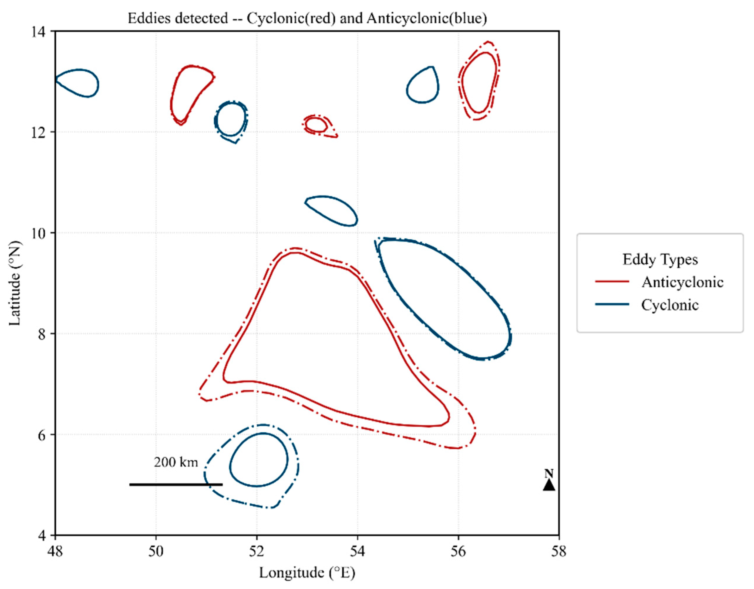
Figure 2.
experimental location. (a) is the Arabian Sea east of the Gulf of Aden, while (b) is the experimental Sea area.
Figure 2.
experimental location. (a) is the Arabian Sea east of the Gulf of Aden, while (b) is the experimental Sea area.
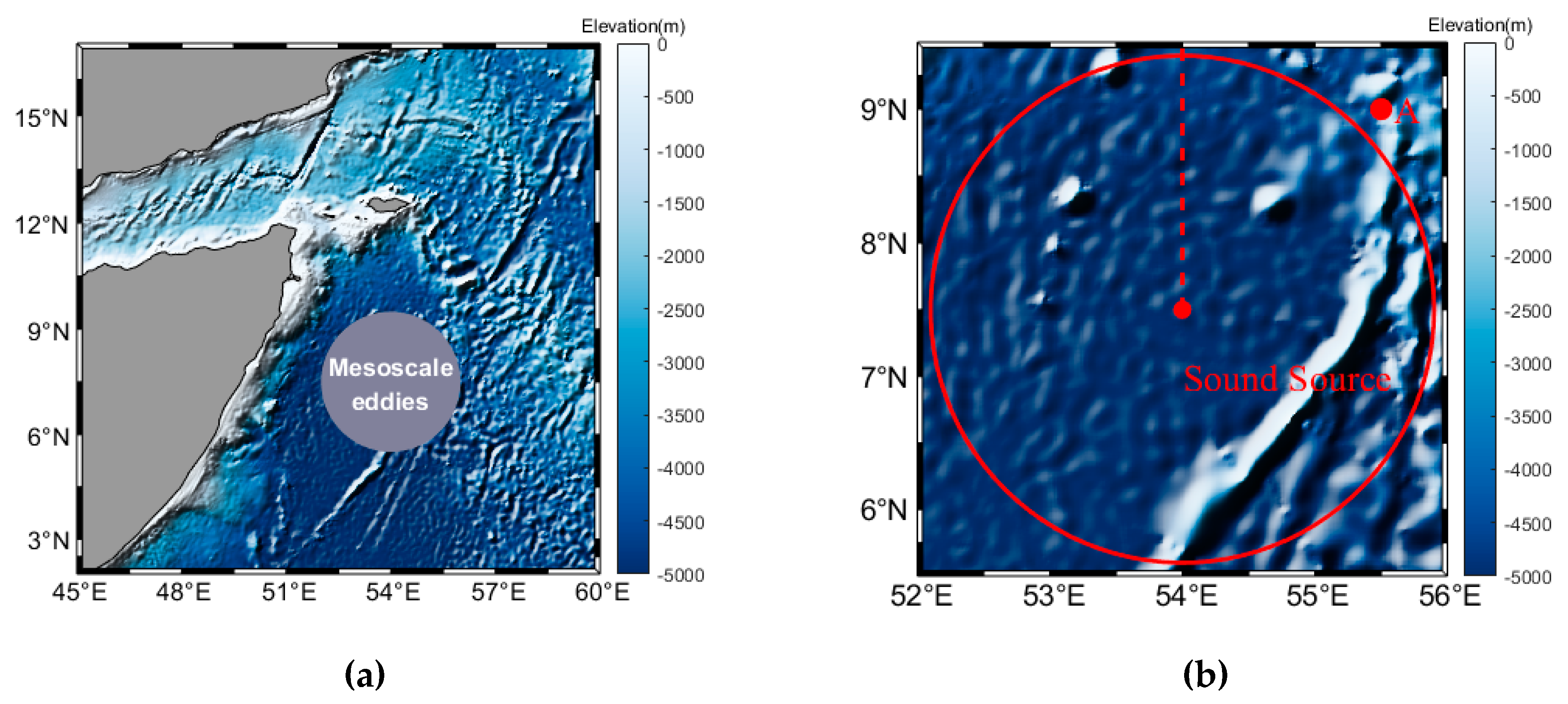
Figure 3.
Eddy Acoustic Velocity Field. (a)-(i) represent the distribution of sound velocity at different depths.
Figure 3.
Eddy Acoustic Velocity Field. (a)-(i) represent the distribution of sound velocity at different depths.
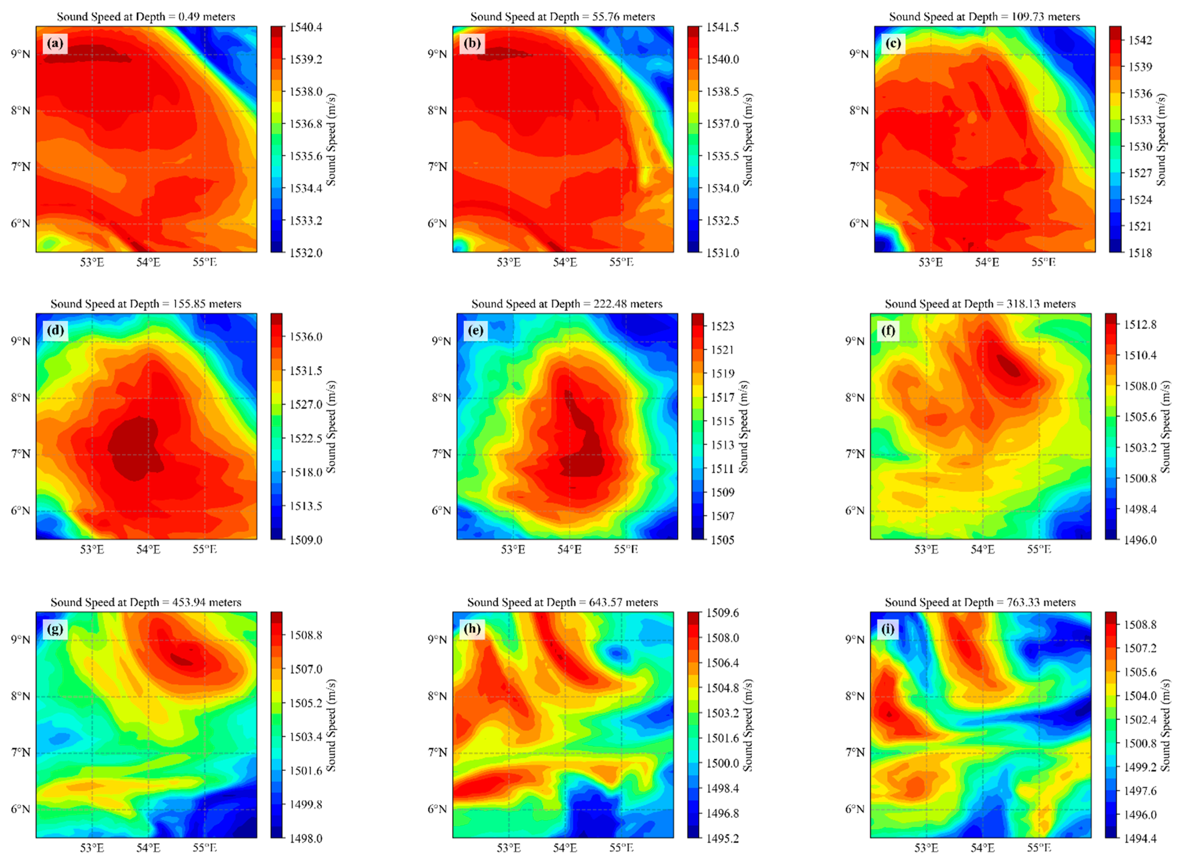
Figure 4.
Figure 4. (a) Abnormal distribution of sound speed along 54° E. (b) Abnormal distribution of sound speed along 7.5° N.
Figure 4.
Figure 4. (a) Abnormal distribution of sound speed along 54° E. (b) Abnormal distribution of sound speed along 7.5° N.
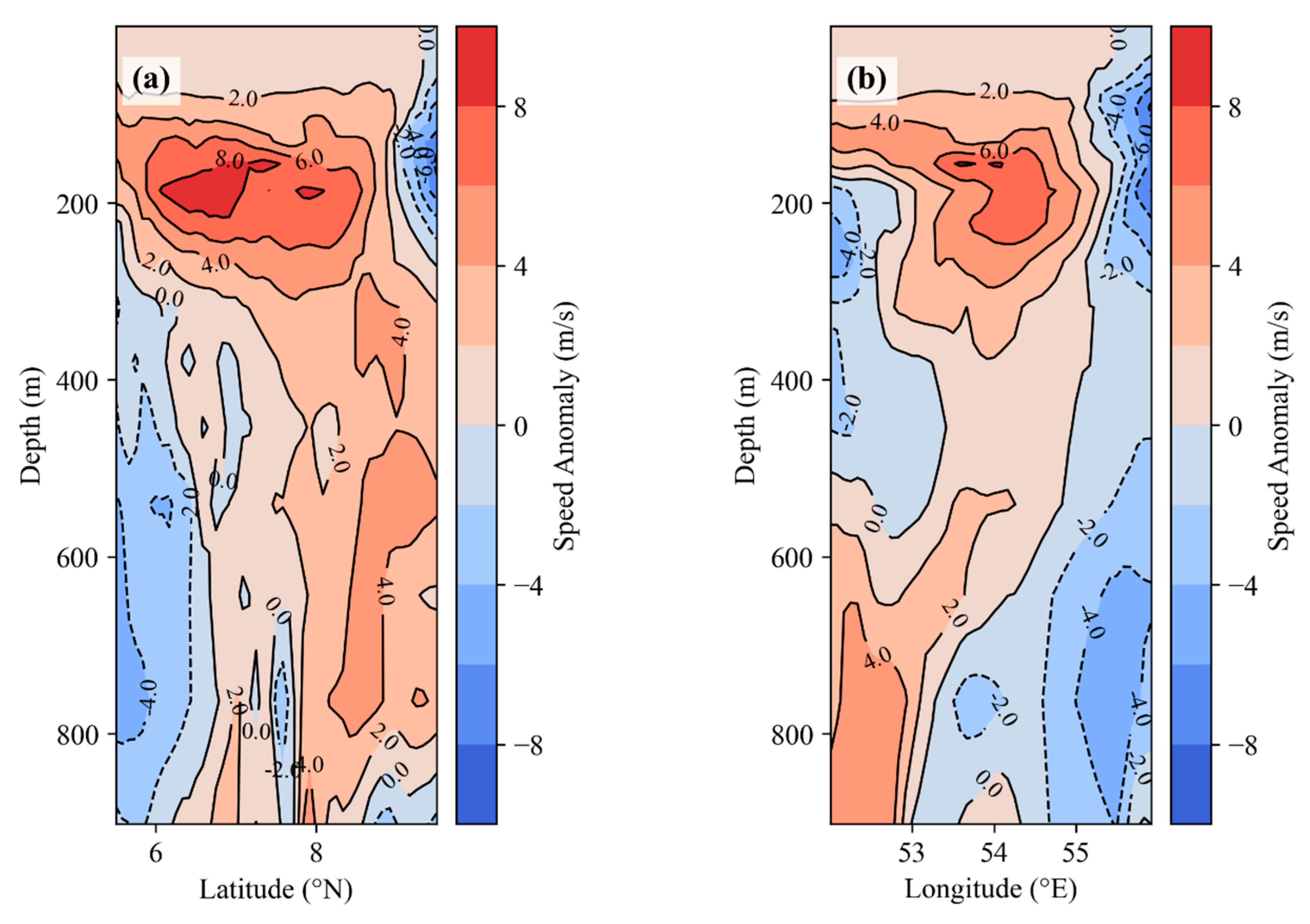
Figure 5.
SWAN-Derived Significant Wave Heights and Strategic Deployment of Directional Wave Spectra Sensors.
Figure 5.
SWAN-Derived Significant Wave Heights and Strategic Deployment of Directional Wave Spectra Sensors.

Figure 6.
Numerical Simulation of One-Dimensional Static Rough Sea Surface.
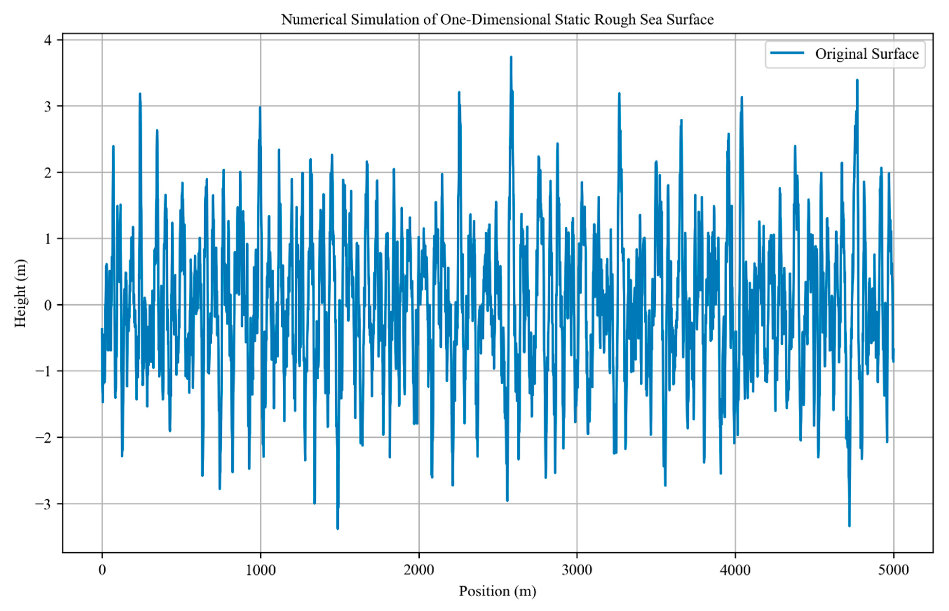
Figure 7.
Comparison of Jason-3, SWAN, and PM Spectrum Results.
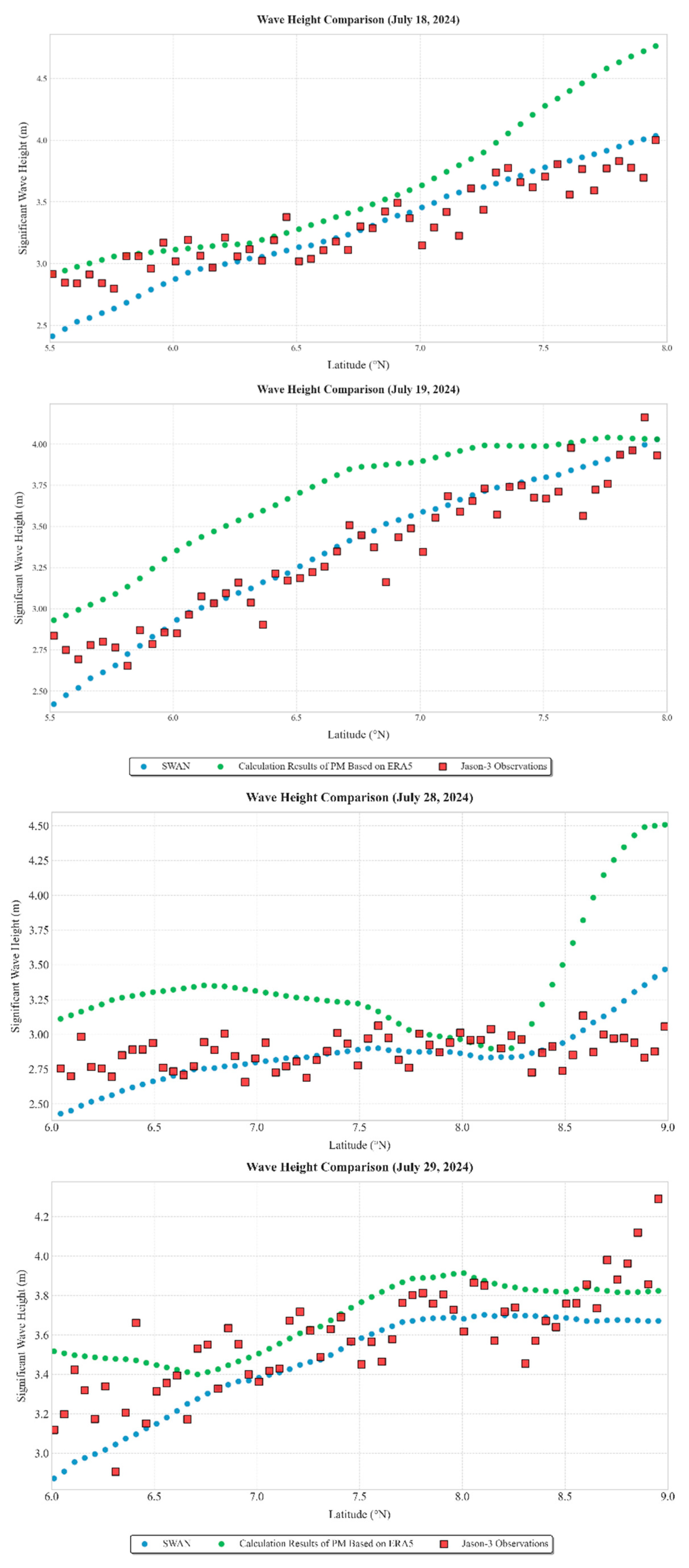
Figure 8.
Comparative Analysis of Sound Velocity Profiles Within and Outside the Eddy Core.
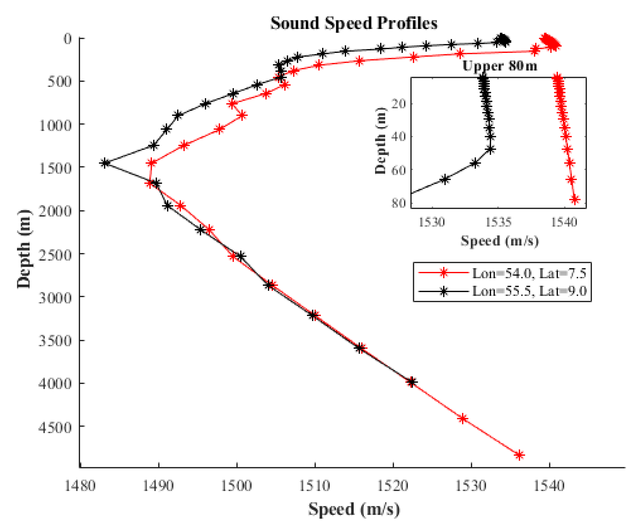
Figure 9.
Propagation Loss Profiles at Three Depths Under Baseline Conditions.; (a) Surface duct; (b) Convergence zone; (c) Deep SOFAR.
Figure 9.
Propagation Loss Profiles at Three Depths Under Baseline Conditions.; (a) Surface duct; (b) Convergence zone; (c) Deep SOFAR.
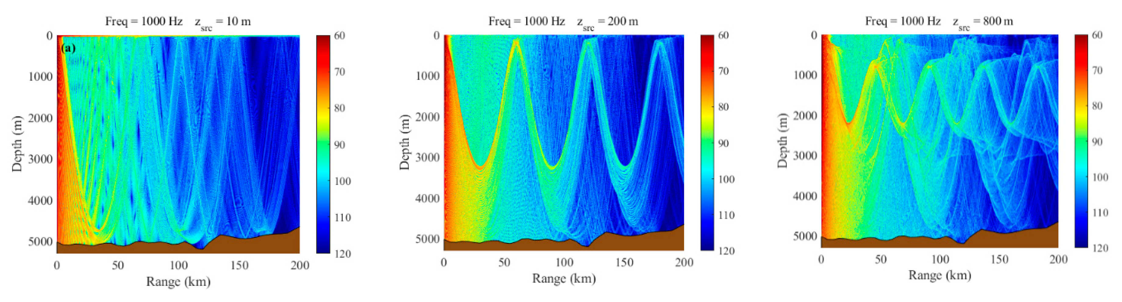
Figure 10.
Depth-Dependent Propagation Loss Analysis in Experiment 2. (a) at 10m south depth; (b) at 200m south depth; (c) at 800m south depth;.
Figure 10.
Depth-Dependent Propagation Loss Analysis in Experiment 2. (a) at 10m south depth; (b) at 200m south depth; (c) at 800m south depth;.
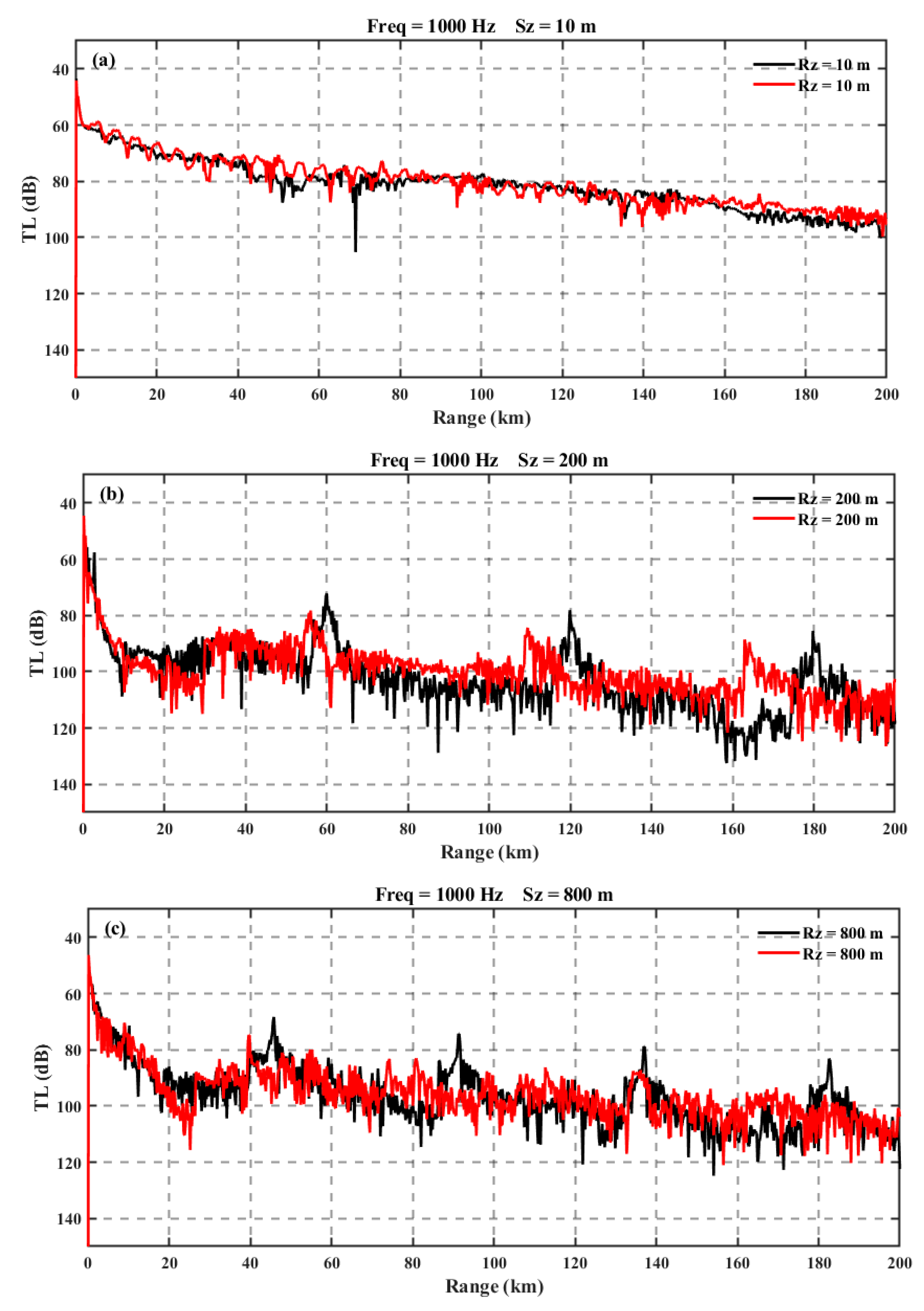
Figure 11.
Ray Path Analysis of Convergence Zone Propagation Mechanisms. (a) Ray Distribution Patterns Under Baseline Condition; (b) Ray Distribution Patterns Modulated by Eddies.
Figure 11.
Ray Path Analysis of Convergence Zone Propagation Mechanisms. (a) Ray Distribution Patterns Under Baseline Condition; (b) Ray Distribution Patterns Modulated by Eddies.
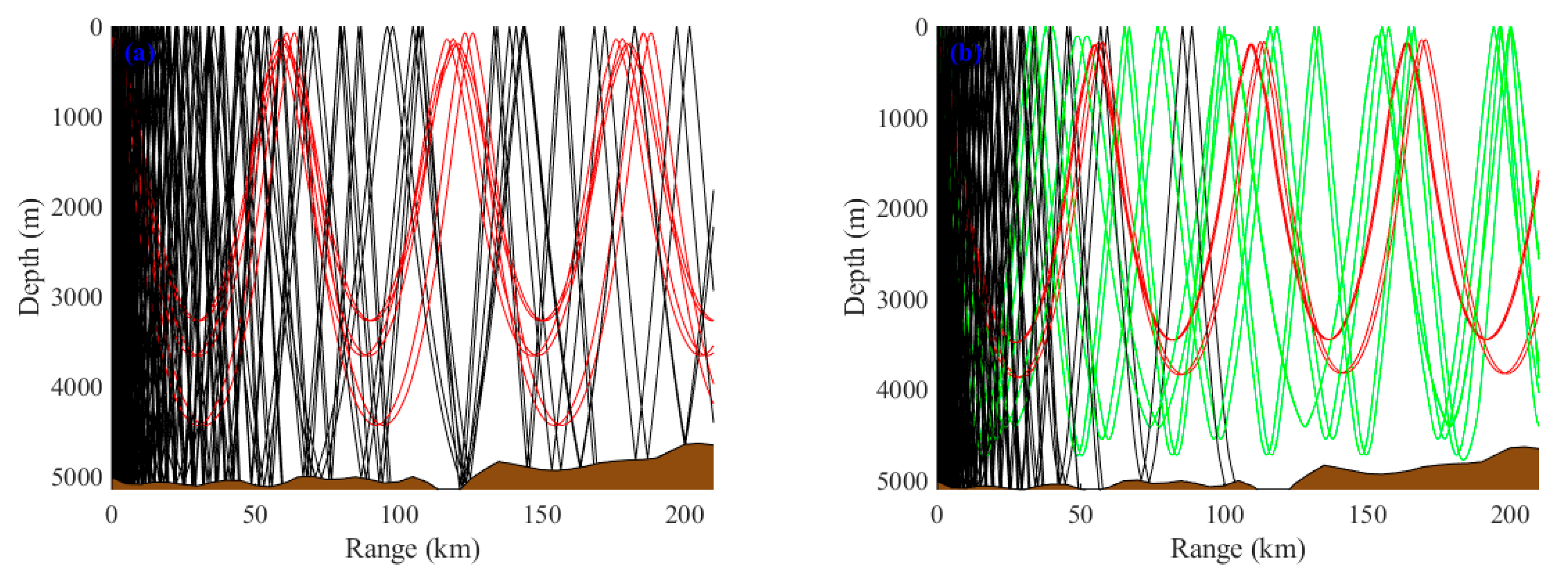
Figure 12.
Experimental Observations of Transmission Loss at 10 Meters Depth. (a) TL under baseline condition; (b) TL under rough sea surface condition.
Figure 12.
Experimental Observations of Transmission Loss at 10 Meters Depth. (a) TL under baseline condition; (b) TL under rough sea surface condition.
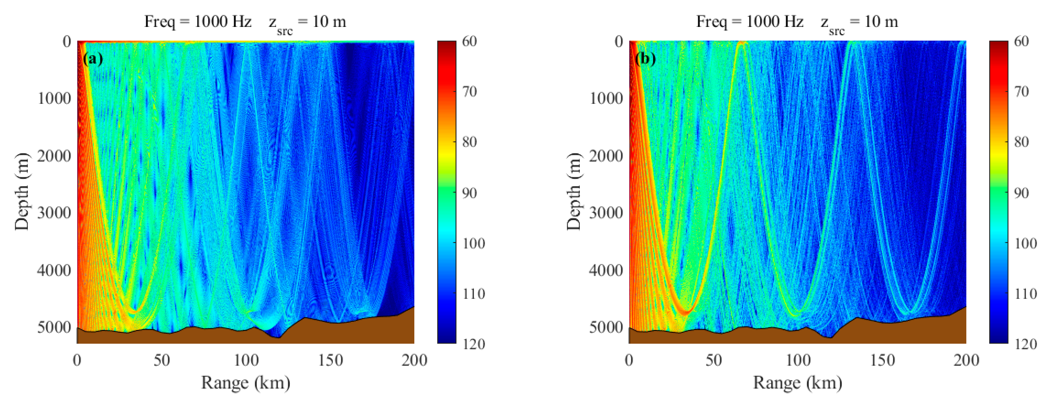
Figure 13.
Comparative Analysis of Horizontal Transmission Loss at 10m Source Depth Between Experiment 1 and 3.
Figure 13.
Comparative Analysis of Horizontal Transmission Loss at 10m Source Depth Between Experiment 1 and 3.
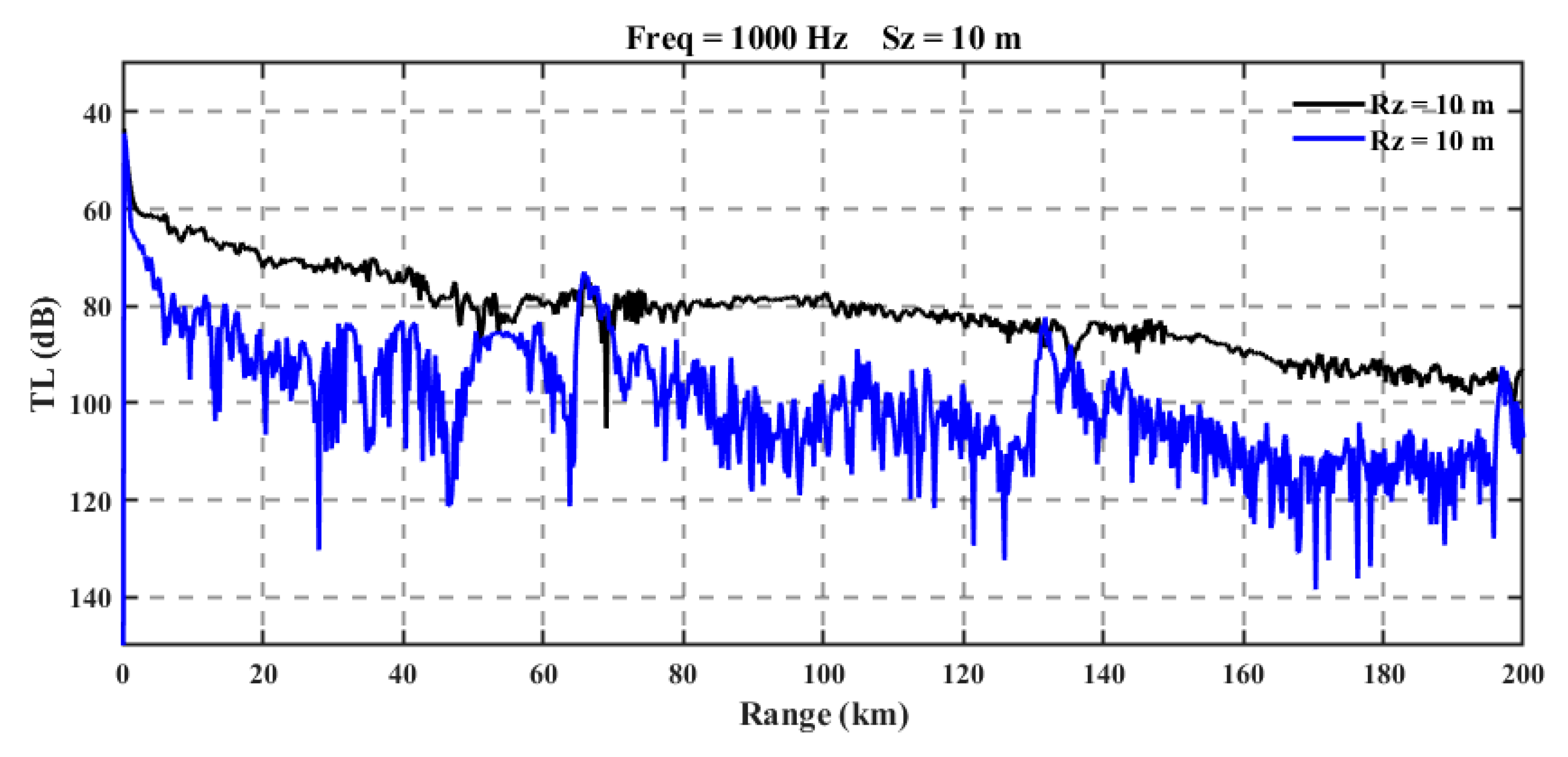
Figure 14.
Comparative vertical profiling of transmission loss between Experiment 1 and 3. (a) at 200m south depth; (b) at 800m south depth.
Figure 14.
Comparative vertical profiling of transmission loss between Experiment 1 and 3. (a) at 200m south depth; (b) at 800m south depth.
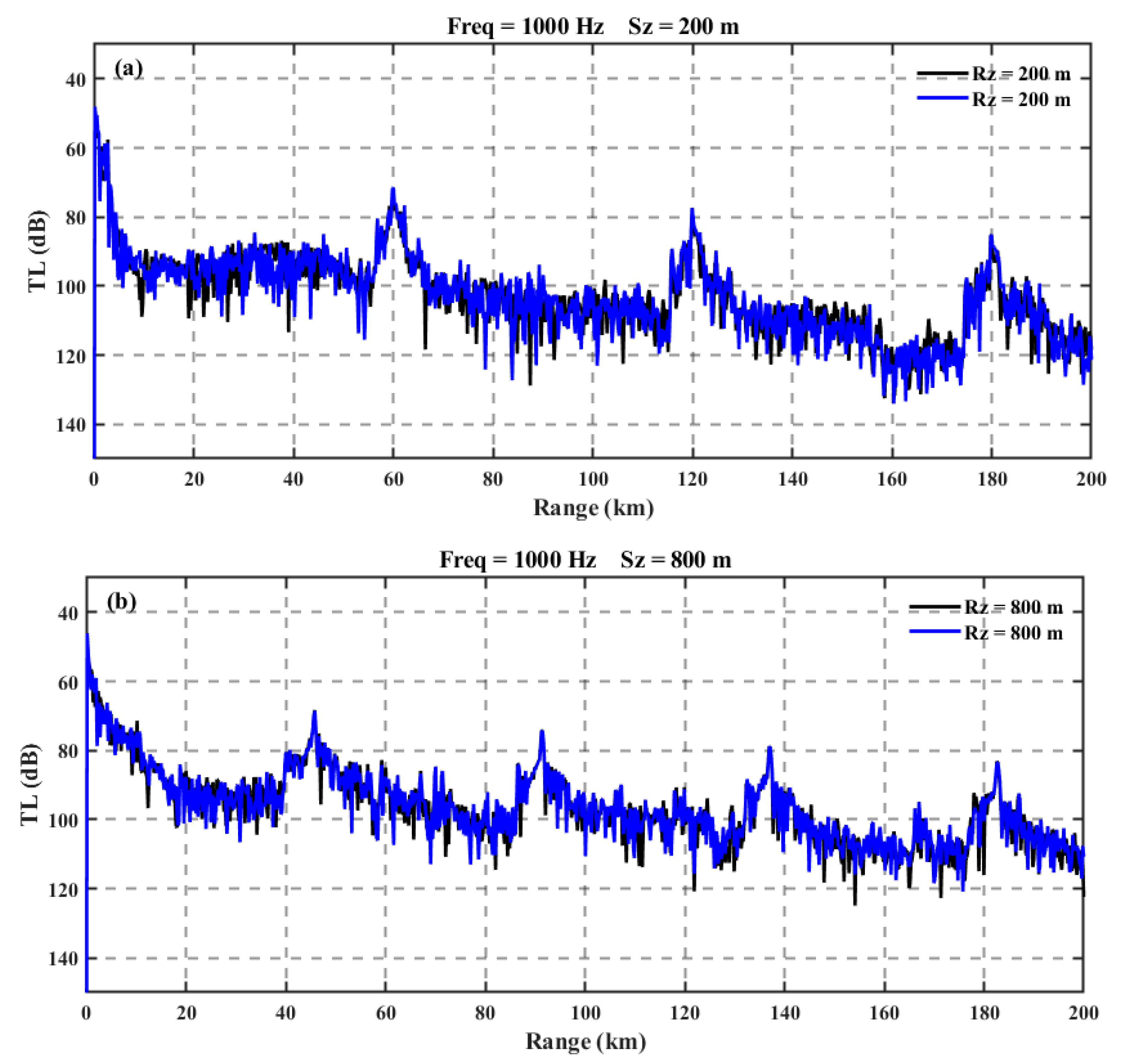
Figure 15.
Comparison of Underwater Sound Propagation Loss in Four Distinct Experimental Conditions. (a) at10m south depth; (b) at 200m south depth; (c) at 800m south depth.
Figure 15.
Comparison of Underwater Sound Propagation Loss in Four Distinct Experimental Conditions. (a) at10m south depth; (b) at 200m south depth; (c) at 800m south depth.
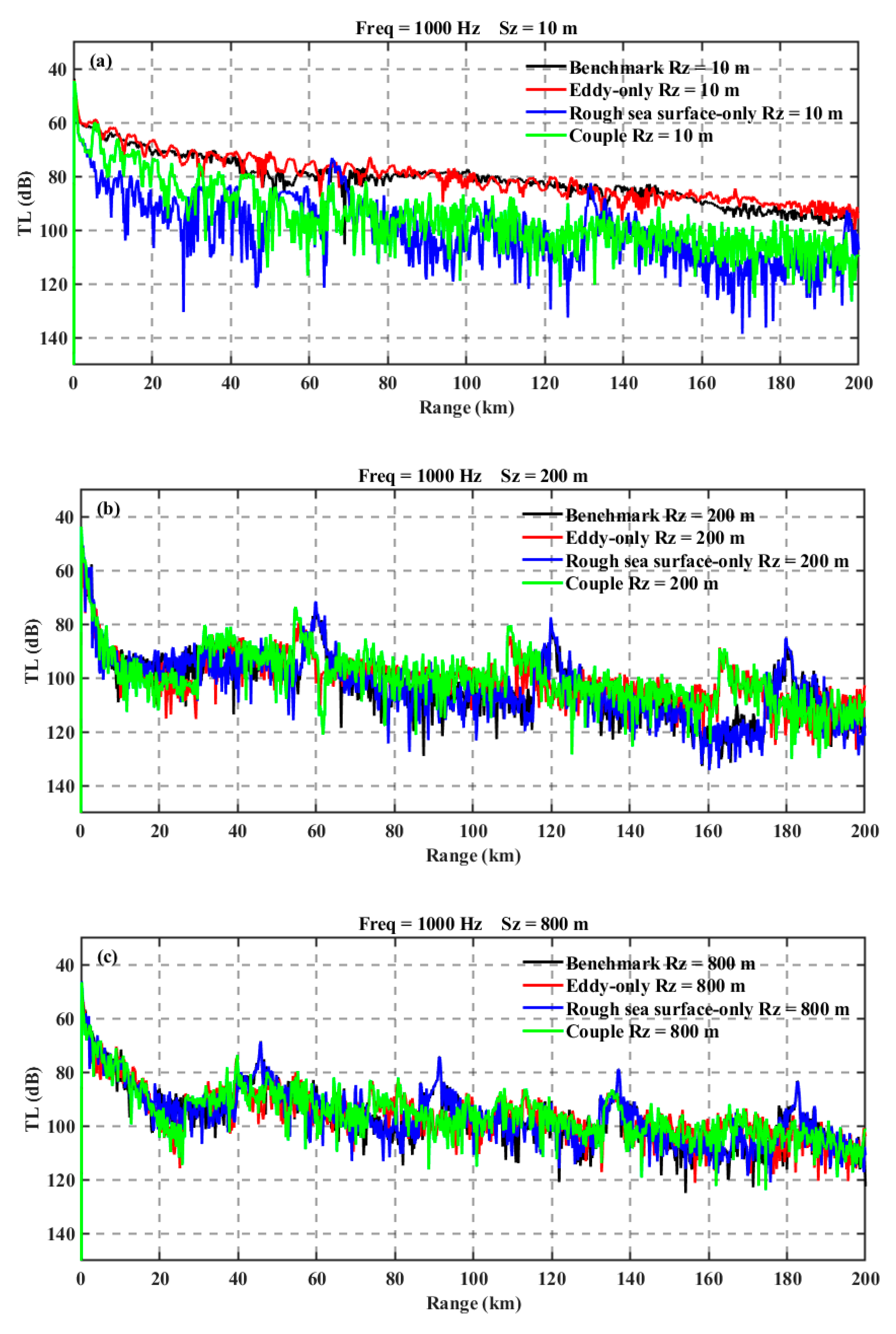
Figure 16.
Mechanistic Transition at 40m Source Depth: Comparative Analysis of Acoustic Propagation Modes Across Four Experimental Conditions.
Figure 16.
Mechanistic Transition at 40m Source Depth: Comparative Analysis of Acoustic Propagation Modes Across Four Experimental Conditions.
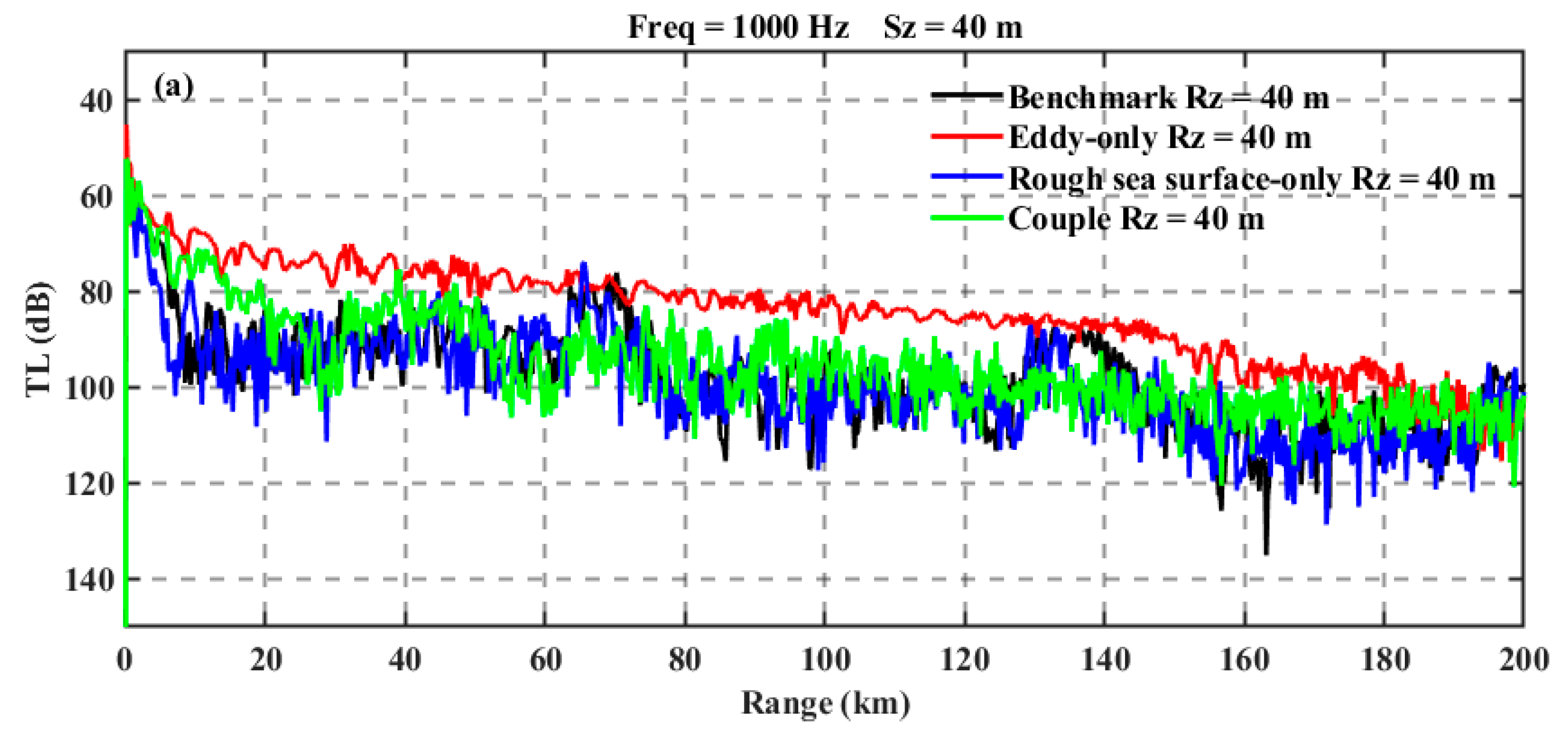

Table 1.
Key Parameter Matrix for Underwater Sound Propagation.
| Parameter | Value | Physical Implication |
| Source Frequency | 1 kHz | high frequency sound wave |
| Source Depths | 10/200/800 m | Surface duct/Convergence zone/Deep SOFAR |
| Bottom Density | 1.3 g/cm³ | Sandy sediment characteristics |
| Bottom Sound Speed | 1600 m/s | Geoacoustic inversion results |
| Attenuation Coefficient | 0.6 dB/λ | High-frequency scattering loss |
Table 2.
Set-up of the four sound propagation experiments.
| Sub-Experiment | With Eddy | With Tide | Purpose |
|---|---|---|---|
| Baseline | F | F | Reference for the following experiments |
| Pure eddy | T | F | Study the effect of eddy only without rough sea surface |
| Pure roughness | F | T | Study the effect of rough sea surface only without eddy |
| Couple | T | T | Study the effect of eddy coupled with rough sea surface |
Disclaimer/Publisher’s Note: The statements, opinions and data contained in all publications are solely those of the individual author(s) and contributor(s) and not of MDPI and/or the editor(s). MDPI and/or the editor(s) disclaim responsibility for any injury to people or property resulting from any ideas, methods, instructions or products referred to in the content. |
© 2025 by the authors. Licensee MDPI, Basel, Switzerland. This article is an open access article distributed under the terms and conditions of the Creative Commons Attribution (CC BY) license (http://creativecommons.org/licenses/by/4.0/).
Copyright: This open access article is published under a Creative Commons CC BY 4.0 license, which permit the free download, distribution, and reuse, provided that the author and preprint are cited in any reuse.


