
Submitted:
19 June 2025
Posted:
20 June 2025
You are already at the latest version
Abstract
Steel is an important product in many engineering sectors, however, the steelmaking industry is one of the largest CO2 emitters. Because of this, new governmental policies push the steelmaking industry toward a cleaner and more sustainable operation. Becoming carbon neutral, utilizing more scrap is one of the feasible solutions to achieve this goal. However, because of the heterogeneity of the scrap in size, shape, and composition, knowledge gaps need to be dealt with to assess the influence of increasing scrap ratio on the Basic Oxygen Furnace (BOF) steelmaking operation. In the context of steel production, understanding heat transfer and the melting behavior of the scrap in the BOF is crucial for two reasons. First, better heat transfer contributes to efficient energy utilization, reduces scrap melting time which potentially leads to more scrap content, prevents non-homogeneous temperature distribution, and improves the BOF operation and lifetime. Second, understanding the melting behavior of the scrap helps designing a better scrap charging process which will lead to a homogenized melt (if good mixing was not applied). The present study is divided into two parts. First, the difference in melting behavior with emphasis on the melting of a single metal element (e.g., Rod, Sphere, Prism) under the influence of natural and forced convection conditions and their corresponding correlations is highlighted. Also, the influence of solid fraction on the melting and the heat transfer process is emphasized. Secondly, a comparison between the utilized numerical modeling approaches is made. It shows that CFD-DEM (Computational Fluid Dynamics-Discrete Element Method) approach offer attractive features compared to traditional Computational Fluid Dynamics (CFD), especially modeling different scrap shapes and types and using of different contact models (e.g., linear - spring dashpot, Hertz-Mindlin). Furthermore, it is computationally cheaper compared to the Particle Resolved Direct Numerical Simulation (PR-DNS). However, to accurately model the scrap melting (and dissolution) a reliable heat (and mass) correlation model is needed to predict the melting (and dissolution) phenomena correctly. Even though DEM has the capability to model the swelling behavior (particle growth or shell formation), the current review shows that there is no model in CFD-DEM available in literature to capture both shell formation (growth) and melting of the scrap.
Keywords:
CFD
; DEM
; CFD-DEM
; Scrap
; Melting
; BOF
; Heat and Mass Transfer Correlation
1. Introduction
Over the past decades, there has been a significant increase in steel production. In 2023 the total production of crude steel in the world has reached 1888.2 Mt [1]. Mainly, of this production originates from the blast furnace (BF) – basic oxygen furnace (BOF) route. BF – BOF route is associated with high emissions, averaging about 2 tons per ton steel. This is approximately four times higher than emissions from production with Electric Arc Furnaces (EAF) [1]. To achieve circularity and net zero emission, future Direct Reduced Iron (DRI) based technologies will play a very important role and are being adapted for direct use of hydrogen. Scrap being an input material with lower emission is one of the solutions to mitigate emissions. Steel scrap is used both in BOF as part of the ferrous input, and in EAF as input material. However, introducing scrap in BOF comes with challenges, such as potentially deteriorating the final steel quality as a result of introducing unwanted tramp elements . In addition, the utilization of scrap in BOF is limited due to unavailability of external energy source to melt the scrap. Therefore, the heat cycle has to be planned carefully based on the details of the final product, hot metal, and scrap quality/composition. The heat cycle in BOF starts by charging different scrap sizes and types. Subsequently, the furnace is pivoted back and forth (rocked) to evenly distribute the scrap on the bottom of the converter and avoid the formation of scrap iceberg (scrap being above the hot metal interface) during the oxygen blowing. Before introducing the oxygen lance to refine the melt (also known as the blowing stage), the converter is tilted back to charge the hot metal. Finally, the refined crude steel is tapped for further processing (secondary steelmaking). During the blowing, large amount of heat and CO ( in post-combustion) is produced as a result of exothermic reactions. Therefore, simultaneous momentum, heat and mass (bottom stirring, scrap melting, dissolution of carbon from scrap and the exothermic reaction products) transfer phenomena prevail during the operation. From a mathematical point of view, the non-dimensional form of the momentum and energy equations introduces a group of dimensionless numbers as Reynolds (Re), Prandtl (Pr), and Nusselt (Nu) numbers (see reference [2] chapter 13). Some of these dimensionless numbers appears in equation of changes (e.g., Re and Pr) and others in the boundary conditions (e.g. Nu). For a sphere immersed in hot metal, the dimensionless quantity () in Equation 1 can be used to describe both the temperature (T) and concentration () profiles. The dimensionless time () expressed as () (c is the thermal or the molecular diffusivity coefficient for temperature or concentration transport respectively) also known as Fourier () number.
On the other hand, the moving solid-liquid interface (R) in the presence of convection, considering different densities and thermal conductivities of the scrap (, ) and the hot metal (, ) at the melting temperature () is described by the dimensionless Equation 2.
It is important to emphasize that the Stefan number
depends on the carbon concentration in scrap-hot metal system. This is because the melting temperature () is not a constant rather it’s a function of the carbon concentration () which can be obtained from the phase diagram for a given scrap composition. Table A1 summarizes the relevant dimensionless numbers for heat and mass transfer problem. Figure 1 illustrates the source of different dimensionless numbers and their relation to scrap and hot metal in the BOF system.
The dependency of the Nu and Re numbers on the characteristic length scale (L) requires a prior knowledge of the scrap shape, which is essential for estimating their average values. Hence, estimating the average external heat transfer coefficient (h). Which quantifies the convective heat transfer per unit mass for each unit temperature in solid-fluid systems.
Due to the similarity between heat and mass transport equations, the heat (h) and mass (hm) transfer coefficients are described by analogous dimensionless correlations [3]. While these coefficients can be analytically determined for simple systems using boundary layer approaches (e.g., flow over horizontal plate) [4], they must be experimentally estimated for complex systems. There are various empirical and semi-empirical correlations have been developed to characterize these coefficients. These correlations are typically expressed in terms of dimensionless numbers Nu, Re and Pr or equivalently Sh, Re and Sc for mass transfer as shown in Equation 4.
It is worth mentioning, that the Prandtl number of liquid metals is very small (order of 0.01) compared to other fluids (e.g. order of 10 for water). This characteristic nature of liquid metals implies that the thermal boundary layer is larger than the momentum boundary layer. This affects the exponent of the Prandtl number in the dimensionless Equation 4. The exponent tends to be larger for fluids with low Prandtl number (e.g., liquid metal) compared to other fluids (e.g., water) [3]. Furthermore, the temperature variation during the heat cycle (ranging between to ) has a considerable influence on the thermophysical properties of the system [5]. Therefore, for a steady-state flow of the hot metal over a scrap piece, the Nusselt (Nu) number depends on the characteristic length (L) of the scrap, variation of the thermophysical properties (Pr), the nature of the hot metal flow (laminar or turbulent) and the heat convection type (natural or forced).
The aforementioned transport coefficients are essential for determining the scrap melting rate in BOF steelmaking process. Inefficient heat and/or mass transfer can cause scrap agglomeration due to shell formation in a dense systems (i.e. at 0.38 dense scrap pile), leading to longer melting time [6,7] or unmelted scrap at the end of the tapping. Hence, caution must be taken when different sizes, shapes, and types of scrap are introduced.
To correctly quantify the melting rate of scrap with different sizes (L, and ) and types (Ste), flow characteristics (Re), temperature (Nu), and species (carbon) concentration distributions (Sh) at the local scale must be measured or predicted accurately. Different melting experiments have been performed to estimate heat, and mass transfer coefficients (e.g., Nu, and Sh) [8,9,10,11,12,13,14,15,16]. However, these experiments are limited to simple shapes (e.g., rods, spheres), single materials type (e.g., steel, ice), and constant temperatures. Such limitations favor the use of numerical approaches to model the melting and dissolution of complex scrap shapes. There are different scales to model the current process [17]. The scale range varies between macro (e.g., Two Fluid Model) to meso (e.g., CFD-DEM) to micro (e.g., PR-DNS) scale see reference [18,19] for different modeling approaches.
In the particulate systems, Particle Resolved Simulation (PR) has proven to be a reliable approach to capture different transport phenomena [20,21,22,23,24]. However, it is computationally unfeasible for such large systems. Alternatively, particle unresolved modeling approaches such as Computational Fluid Dynamic coupled with Discrete Element Method (CFD-DEM) or Two-Fluid Model (TFM) are computationally cheaper, but they require closure relations for the multiphase mass, momentum and heat transport. In CFD-DEM approach, heat and mass transfer phenomena are evaluated using semi-empirical correlation (e.g., Gunn’s relation [25]).
In the context of scrap-hot metal interaction, the used semi-empirical correlation should fulfill the following criteria. First, the correlation should be applicable to the operational conditions in the BOF. In other words, the correlation should be relevant within the Reynolds and Prandtl number range of the flow and temperature during the process. The flow conditions and temperature of the hot metal vary during the operation, starting at charging hot metal to gas stirring via bottom tuyeres, and to top lance blowing. It is expected that forced convective heat transfer prevails at the beginning of the hot metal charging [26], followed by natural convection until the agitation of the hot metal bath starts using bottom tuyeres and the oxygen lance. Secondly, estimation of the Reynolds number for scrap particles, requires specification of a characteristic length of the actual scrap with a complete shape. It is worth noting that scrap size will increase at the initial time due to shell formation (solidification of the melt on the scrap) unless the scrap is preheated (to approximately [27]). Thirdly, the correlation should account for the influence of solid fraction of the scrap pile as it influences the heat transfer analogous to drag force in dense granular systems [28]. Finally, it should be valid for low Prandtl number of liquid hot metal (order of ).
To understand the above mentioned criteria, relevant heat and mass transfer correlations for both natural and forced convection are listed and assessed in the next section. Furthermore, the influence of the solid fraction of the scrap bed (porosity) on the transport coefficients will be addressed. Finally, different modelling approaches with emphasis on CFD-DEM applicable to model the BOF process are outlined. Through this, the relevant existing heat and mass transfer correlations for low Prandtl numbers are reviewed and the impact of the solid fraction of the scrap bed on the transport coefficients within the CFD-DEM framework is highlighted.
2. Experimental Studies of Scrap Melting
Many experimental works found in literature investigate the melting behavior of steel scrap [8,12,14]. However, these investigations are limited to a single melting object (e.g., sphere or a rod), or multiple similar objects distributed randomly [29], or systematically [6,7]. Some studies use alternative materials such as water and ice (also known as cold models) [11,30,31], aluminum [32], or zinc [10] to perform similarity analysis of the scrap melting in liquid hot metal. Some of these alternative material (e.g. cold models) offers the possibility of performing experiments with advanced measuring techniques (e.g., particle image velocimetry (PIV)) to estimate the melting rate accurately).
On the other hand, industrial-scale experiments remain scarce due to the difficulty of obtain uniform scrap input (e.g., size and shape, and composition) and experimental data during the heat cycle. Furthermore, the lack of non-invasive techniques at high temperature conditions () poses extra safety concerns. In the BOF, both mass and heat transfer occur during the heat cycle, and the rate of heat and mass transfer varies during the cycle as a result of the exothermic reactions [18], as well as the stirring (and oxygen blowing) conditions of the hot metal bath [33]. The latter defines the nature of the external heat and mass transfer processes. For a flow driven by a concentration (or density) gradient the convective heat transfer is natural. Whereas, forced convective arises when the flow results due to the action of external forces. The following sub-sections summarize the experimental studies in natural and forced convection and their corresponding correlations. While the last sub-section highlights the influence of the solid fraction in the scrap pile and its influence on the melting rate.
2.1. Melting in Presence of Natural Convection
The natural (free) convection happens due to buoyancy forces caused by density differences in the fluid [34]. These differences are usually initiated by temperature, or concentration gradients or a combination of both.
For a heated vertical plate, these temperature gradients create density differences between the bulk fluid and the fluid near the plate surface. These differences induce buoyancy forces and lead to fluid motion. The dimensionless form of the conservation equations of mass, momentum and energy gives a set of dimensionless numbers. These dimensionless numbers are Reynolds, Prandtl and Grashof . The Grashof number represent the ratio of the buoyancy force to the viscous force. The nature of the convection is determined by the ratio of Gr and Re as following [34]: natural convection is dominant if , forced convection is dominant if and mixed (combined) convection for . From the solution of the boundary layer equations for a vertical plate, the Nusselt number (heat transfer coefficient) can be expressed as a function of Prandtl and Grashof numbers [3,34] as in Equation 5
Even though heat and mass transfer are similar phenomena, there is still less attention given to the strong coupled-nature of these two in the BOF. Such strong coupling is attributed to the large heat produced during oxygen blowing. As a simplification researchers tend to study these phenomena individually assuming small gradients in the neglected key variables.
Churchill [35] developed correlation 10 given in Table 1 for a single sphere to estimate the heat transfer coefficient for natural convection for laminar flow conditions. The correlation is valid for all ranges of Prandtl and Grashof numbers. Argyropoulos et al. [16] conducted a similar work on liquid metals for a single sphere under natural and forced convection. Argyropoulos performed experiments on aluminum and steel spheres submerged in their respective melts. The set up consisted of a stationary melt to mimic natural convection heat transfer. Argyropoulos stated that correlation 11 showed a better fit to the experimental results compared to Churchill [35] and Raithby [36] correlations. However, the range of the experiments is too narrow to generalize this statement. Shell formation was observed by recording the temperature profile at the center of the sphere. The temperature profile was flat for the first 10 seconds and later started to increase, indicating the starting of the melting of the sphere. This shell formation delays the melting of the scrap, which is not favorable in BOF process. An earlier work of Ehrich et al. [9,37] attempted to estimate the shell size and the melting time analytically of a sphere by solving the heat transfer equations in the spherical coordinate system. The model consisted of a concentric shell and core of different materials. They were able to identify two limiting cases for such a system. First, when the thermal conductivity is equal to zero, the melting profile is linear, and no shell is formed. Second, for a high thermal conductivity (close to infinity) shell size reaches approximately of the initial radius. Perez et al. [38] modified the model of Ehrich to account for the variation of heat transfer coefficient and the thermophysical properties. The modified model showed larger shell sizes compared to Ehrich model. It is important to emphasize that the experimental results of Ehrich et al. did not capture the shell formation while Perez’s experiments successfully did. Figure 2 shows the normalized melting profile of a sphere whose initial radius is 0.975 cm. The observed increase in size is due to the shell formation, which is influenced by the temperature difference, thermophysical properties and heat transfer coefficient.
Many experiments have been conducted on single vertical rod immersed in hot metal. However, Nusselt correlations for vertical rods are obtained using approximations valid for vertical flat plate configuration [39]. Fujii et al. [40] used the local Nusselt number based on a vertical plate correlation to estimate the local Nusselt number for a vertical cylinder. A common method of obtaining the Nusselt number for vertical cylinders uses the thin boundary approximation as explained in reference [41]. For a vertical cylinder in a laminar flow, the Nusselt number is given by correlation 6.
where is the Nusselt number for a thick laminar boundary layer on a plate of the same length as the cylinder and obtained using the following correlation:
Here, is the Nusselt for a thin boundary layer on a plate of the same length obtain from correlation Table 1 without the term . The parameter is defined in Equation 8 for a cylinder of length and diameter L and D respectively.
Churchill and Chu [42,43] formulated a Nusselt correlation for natural convection given by Equation 12, applicable to laminar flow for a vertical plate. They indicated that the relation covers a wide range of Rayleigh and Prandtl numbers, and it can also predict the mass transfer. Subsequently, Churchill [44] devised a general Nusselt correlation adaptable to various object shapes. The correlation aims to cover both natural and forced convection regions by taking the ratio between the Nusselt number for natural and forced convection. Churchill and Bernstein [45] attempted to estimate the Nusselt number for a cylinder aiming to cover a wide range of Reynolds numbers (laminar and turbulent). However, they indicated that the relation is not accurate in the intermediate (transition) regime .
Recently, Xi et al. [46] studied experimentally the melting of cylindrical and squared steel bars. The authors did not mention the value of the heat transfer coefficient used in their experiments. Nonetheless, they investigated the influence of the initial temperature of both the melt and the steel bars on the melting. The result revealed that an increase in the initial temperature of the melt decrease the melting time of the steel bars. Hence, confirming the linear decrease of the melting time reported by Li et al. [27]. However, the square bars showed more pronounced shell formation compared to the round bars. This is related to the high surface area of the square bars. Thus, square bars tend to have a longer melting time compared to the round bar. Figure 3 shows mass based normalized melting profiles of both round and square bars at an initial temperature of submerged in a bath of the same material at different temperatures.
The dissolution of steel has been also studied experimentally under isothermal temperatures [8,12,47,48]. Such studies allow the quantification of the mass transfer coefficient due to carbon diffusion from the liquid melt to the solid steel. Szekely et al. [8] used a constant heat transfer coefficient ranging between to study the dissolution rate of steel rods in a hot metal bath. The carbon concentration in the bath and the rods were in the range of and , respectively. The temperature was kept below the melting temperature of the steel rods. They showed that the rod started to melt while the bath temperature was below the melting temperature of the steel. In this case, the melting was driven by carbon diffusion into the steel rod. Additionally, shell formation was observed.
Wright [12] used the results of iron rod dissolution in Fe-C quiescent melt to fit a Sherwood correlation 9 as a function of the Grashof and Schmidt numbers valid for .
The dissolution rate of the rods was estimated from the variation of the rod diameter and the immersion time. Additionally, Wright investigated the influence of the temperature and carbon content of the melt on the dissolution rate. The result of the temperature variation shown in Figure 4 (a) indicates an increase in the dissolution rate as a function of the melt temperature.
Penz et al. [50,51] studied experimentally and numerically the dissolution of steel rods in liquid hot metal driven by the concentration gradient. They investigated the dissolution rate of the steel rod in both static and rotating modes. The modes of the rod are intended to mimic natural and forced convection caused by the flow of the hot metal in the BOF process. Their study revealed that the rate of dissolution using a rotating rod is higher (approximately twice) compared to the static rod under the same conditions. Also, shell formation was observed for almost 10 seconds, concluding that the size of the shell strongly depends on the initial temperature of the rod and the melt. The maximum shell thickness was estimated to amount of the initial radius [49]. They estimated the mass transfer using the liquidus carbon concentration at equilibrium temperature. Figure 4 (b) shows the distorted shape of the melted steel rods at different immersion times [49]. In their numerical work, Penz et al. [52] used the Nusselt correlation 13 given in Table 1 for a vertical rod to estimate the heat transfer coefficient. They solved the heat transfer equation in cylindrical coordinates considering only the variation of the temperature in the radial direction. Their solution showed a higher heat transfer coefficient than the experimental results by a factor of 10. They associated this difference to the shell formation, and the gases trapped between the shell and the rod which reduced the external heat transfer values. Later, Deng et al. [53] indicated that there is also an axial variation of temperature, and it is not constant as Penz et al. [52] assumed. They mentioned that the temperature variation between the top and the bottom introduces a circulation flow between the top and the bottom of the melt. At a later time, the system reaches thermal equilibrium where this circulation flow is driven by the concentration gradient.

Table 1.
Average Nusselt correlations for natural convection for sphere, vertical plate, and vertical cylinder valid for low Prandtl number.
2.2. Melting in Presence of Forced Convection
Forced convection heat transfer is present when the flow of the hot metal is driven by pressure difference induced by external sources. Such flows typically lead to a thinner momentum boundary layer compared to the natural convection one. In such conditions, the heat transport is dominated by the convection. One of the earlier studies to estimate the heat transfer coefficient in forced convective flows was conducted by Whitaker [55]. Whitaker developed an empirical correlation given in Equation 14 for flow past a single sphere.
The above correlation is valid in the range of , and for , and respectively. Whitaker assumed constant thermophysical properties of the fluid, except for the viscosity. This means that the heat transfer coefficient is a function of the fluid viscosity at different temperatures of the system. The viscosity ratio is estimated at the bulk fluid temperature and at the surface temperature of the sphere. Ranz-Marshall [56] developed correlation 15 for the evaporation of single drops valid for Reynolds and Prandtl numbers in the range of and , respectively.
Argyropoulos et al. [16] investigated the sensitivity of Nu correlation to low Prandtl values by fitting a semi-empirical correlation 22 to steel and aluminum experiments data for a sphere in its melt. The exponent of the Prandtl number in the correlation 22 was found to be higher than the one in Hsu, Sideman (see reference [16]), Whitaker and Gunn’s correlations. It is noteworthy that correlation 22 produced a better fit when it was compared to Hsu and Sideman correlations. Figure 5 shows the experimental results of aluminum (triangles) and steel (circles) for Sideman and Hsu correlations (lines b, and c respectively) with Argyropoulos et al. [16] correlation (line a). In addition, Argyropoulos et al. [32] observed shell formation, and estimated the mass increase of the sphere to be between and . This estimation of the shell thickness is high compared to the results of Xi et al. [46] and Li et al. [27]. Nonetheless, it is still within the calculated range of Ehrich et al. [9]. Both Aziz et al. [57] and Hao et al. [30] did not report shell formation for ice-water system with temperature difference and ice being at . Melissari and Argyropoulos [13] developed a dimensionless correlation 16 based on theoretical study for immersed sphere over a wide range () of low Prandtl numbers and applicable in the range of () for Re. The power of the Prandtl number in the correlation is still higher than Whitaker and Gunn’s but it is lower than the experimental fitted correlation 22. A direct numerical simulation was conducted by Rodriguez et al. [58] to evaluate different theoretical and experimental based correlations.
Their simulation results revealed that correlation 22 underestimates the heat transfer coefficient while correlation 16 overestimates it. It is worth noting that Witt correlation 25 performed better than correlation 22 relative to the simulation results.
The bottom blown gas in BOF enhances the melting of scrap. This has been investigated by many researchers [11,31,32,59] in a context of heat transfer of a single sphere in a plume. Iguchi et al. [11] investigated the influence of turbulence intensity of the flow using both water jet and bubbling gas on a single ice sphere. The results indicated high heat transfer in case of the gas plume. The reason is associated to the difference in the turbulence effect induced by the plume jet. This effect reduces the thickness of the boundary layer. Therefore, enhancing the heat transfer and increasing the Nusselt number. Iguchi modified Whitaker correlation to account for the turbulence intensity () by multiplying the left hand side of Equation 14 with . Argyropoulos et al. [32,59] also quantified the turbulence effect of the flow using two spheres of different materials. The spheres were made of aluminum and steel and immersed in their melts. Forced convection heat transfer was induced by means of rotating the sphere and introducing argon gas plume. The results shows that the Nusselt number for the plume is higher than the rotating sphere setup. Hence, confirming the results of Iguchi et al. [11]. The effect of shape variation during the melting on the heat transfer has an influence on the heat flux due to the variation of surface area. Hao et al. [30] studied the effect of shape variation in ice water system using image analysis. The effect of shape variation was quantified by measuring an equivalent surface and volume particle diameters. Small variation between surface based and volume based diameter was observed at the end of the melting time. Nonetheless, the diameter profiles are identical for both surface based and volume based diameters. They developed correlation 17 to calculate the Nusselt number. However, their empirical correlation is only applicable to a narrow range of Prandtl numbers ().
While the above studies focused on the heat transfer coefficient by estimating the Nusselt number, Wright [12] estimated the mass transfer coefficient for melting of steel rods in isothermal system of Fe-C melt. The melt was agitated using nitrogen gas injected at the bottom. Rods of the same radius (6 mm) and different lengths have been used in two different amount of Fe-C melt (with different furnaces capacities). This was necessary to ensure that the initial carbon concentration was not affected by the carbon dissolution into the rods. The dissolution rate under the influence of turbulent forced convection was estimated by plotting the rod diameter versus the immersion time as a function of different gas flow rates. The results revealed a linear relation between the diameter variation and the time for different gas flows, indicating a constant melting rate as shown in Figure 6. The obtained mass transfer coefficient under forced convection was found to be depending on the gas flow rate and more precisely on the plume velocity. Furthermore, the variation of the melting rate between different curves is becoming smaller indicating that an increase of the gas flow rate above a specific flow rate will give rise to poor heat transfer as stated by Wright.
Figure 6.
Dissolution of 6 mm radius steel rods (composition: , , at bath Temperature , and carbon concentration ) in different nitrogen gas flow rates in (a) 1 kg iron bath and (b) 25 kg iron bath [12].
Figure 6.
Dissolution of 6 mm radius steel rods (composition: , , at bath Temperature , and carbon concentration ) in different nitrogen gas flow rates in (a) 1 kg iron bath and (b) 25 kg iron bath [12].
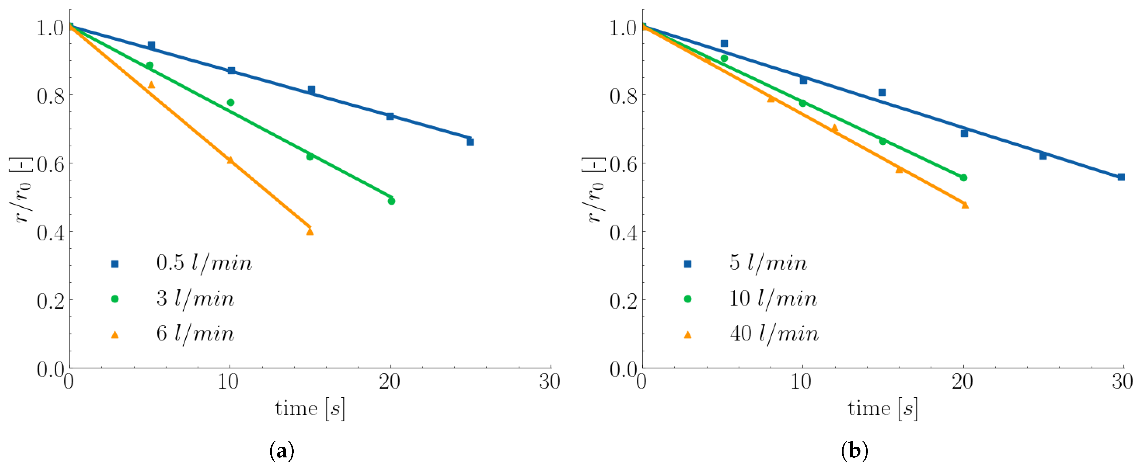
Figure 7.
Melting rods with different stirring aids (a) rod specification: radius r0 = 6 mm, composition: , , bath specification , , stirring gas is Nitrogen [12]. Wei’s rod specification: intial radii () are 10 and 25 mm, composition: , , and molten bath temperature and [60], (b) dimensionless melting profile of a rotating (923 rpm) carbon steel rod (radius mm) immersed in liquid Fe-C at different molten bath temperatures [47].
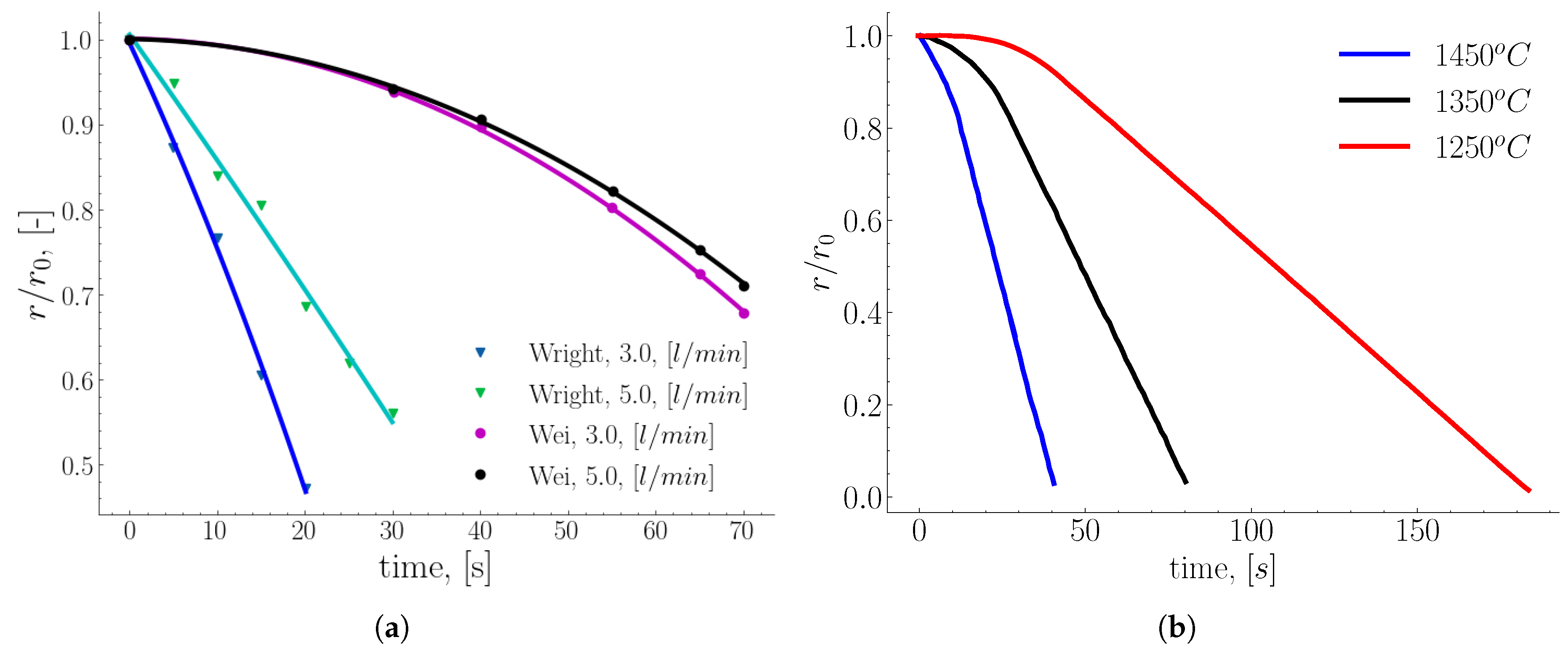
A similar study was reported by Wei et al. [60] to estimate the dissolution of steel rods in 150 kg induction furnace. The rods were immersed in a pig iron melt of carbon content . The melt was agitated using bottom blown nitrogen gas at different flow rates of 3, 5 and 7 l/min. The results of Wei et al. [60] showed an increase of the dissolution rate proportional to carbon concentration gradient and the agitation intensity in accordance with the results reported by Wright [12]. However, from a quantitative point of view, the melting profile obtained by Wei et al. [60] shows a linear melting rate, while the results of Wright [12] show a constant melting rate as shown in Figure 7 (a). It is noteworthy, that the initial carbon concentration gradient for Wei et al. [60] and Wright [12] experiments are and , respectively; while the temperature of the melt for both is . This variation in melting rate could be related to the different composition of the rods. Another study was performed by Isobe [47] to estimate the dissolution rate of steel rods in a 5 ton converter. Isobe modified Lommel and Chalmers correlation [61] to account for small dissolution rate as given in Equation 18.
where () is the moving mass transfer coefficient relative the moving interface. The melting profile of Isobe model for a single rod is shown in Figure 7 (b). Isobe obtained a non-dimensional correlation as given in Equation 19 for a rotated rod.
Furthermore, the melting profile of the rod showed a non-linear trend for the first of the melting time agreeing with The results of Wei et al. [60] and linear profile for the remaining of the melting time similar to Wright [12]. For different shapes other than spheres and cylinders, Kurobe et al. [10] studied the melting process of a prism shape object. The cold model (ice-water) was employed to investigate the melting of a zinc ingot in a hot dip plating bath. A thermal similarity analysis was performed using two correlations applicable for liquid metals and water to estimate the Nusselt value. It is worth mentioning that the equivalent surface diameter of the prism has been chosen as the characteristic length of the prism. They indicated the importance of including the turbulence intensity in the scaling correlations as presented by Equation 20
Also, Shukla et al. [31] performed cold model experiments on different shapes, namely, sphere, cylinder, and plate. Bottom argon gas was used to induce forced convection heat transfer. They found that the melting rate () is not influenced by the shape of the object in contrast to the melting time. Shukla et al. [31] fitted a Nusselt correlation of the form to estimate c and n coefficients for each shape individually and all shapes together. The estimated error in the coefficients for all shapes together for that shown in correlation 21 is greater than the ones obtained for the individual shapes.
This variation could be attributed to the sensitivity of the correlation to the choice of the characteristic length scale. Cao et al. [62] used ice cured with quartz particles in 80 ton water converter. Different sizes of the cured ice (plate shape) were used to model scrap melting in the BOF. The result indicates a better mixing and heat distribution for small scrap pieces. Therefore, the study suggests to avoid large scrap pieces during BOF operation.
2.3. Influence of Scrap Solid Fraction on The Heat Transfer in Liquid Hot Metal
An analogy exists between heat transfer and drag forces in bulk particulate systems [18,25,28]. Just as drag forces can contribute to particle clustering in fluidized beds (alongside other factors such as particle-particle collisions), heat transfer processes lead to the formation of hot and cold zones within the system. Consequently, accurate prediction of heat transfer in high solid fraction systems (characterized by low voidage in scrap piles) is crucial for determining operational stability. Hot/cold zone was observed by Gaye et al. [64] in industrial BOF experiments. They noticed that in some cases the melting time of small scrap pieces is longer than the large ones in a typical converter condition, indicating that temperature was not uniformly distributed over the different scrap pieces.
The influence of the porosity on the Nusselt correlation was indicated by Whitaker. He developed correlation (25) applicable to staggered cylinders and granular systems (e.g., packed bed). However, it is only applicable for porosity (voidage ) less than and Prandtl number and recommended for Reynolds number above 50.
By introducing the porosity (voidage fraction ) as an independent variable in Nusselt correlation, Gunn [25] derived one of the widely used correlations given in Equation 27 for dense systems.
where , , , , and . In contrast to Whitaker[55], Gunn’s correlation is applicable to systems with a porosity range between , and for Reynolds and Prandtl numbers, in the range of , and , respectively. Nonetheless, the sensitivity of Gunn’s correlation to Prandtl variation below 0.6 (e.g., in case of liquid steel) has not been quantified.
Also, Jiang et al.[29] studied the convective melting of a spherical ice packed bed system under both gravity and microgravity conditions. Their results showed that the average Nusselt number of the bulk particle system is less compared to the single particle under identical conditions. It is worth mentioning that the heat transfer in the Jiang studies was enhanced by the convective nature of the flow.
On the other hand, the influence of the porosity in a quiescent melt on the melting dynamics has been investigated by Li et al. [6]. They studied the melting behavior of two and multiple rods in quiescent melt. They classified the influence of the spacing between the immersed rods in hot metal into three melting categories. These categories are: (i) independent melting rods, (ii) partially agglomerate rods, and (iii) fully agglomerate melting rods. This has an important effect on the process operation, since the melting time is not determined by the melting of a single object anymore, rather by the state of the agglomerated objects. Their multi-rods experiment showed that the melting time increases non-linearly with increasing solid fraction. Similarly, Xi et al. [7] studied the melting behavior in porous structures finding that high porosity (near 1) leads to independent melting of the objects, low porosity (below ) results in partially independent melting, and very low porosity causes fully dependent (agglomerated) melting. Their findings further confirmed the results of Li et al. [6]. It is important to point out that in the above studies [6,7] the heat transport was performed under natural convection conditions, while the heat transfer in [24,29,64] was convective melting driven by fluid flow. Because of the influence of porosity variation on the melting time (t). Xi et al. [7] developed a correlation 28 (27) to predict the melting time (t) of multiple objects from the melting time of its single constituent (). The correlation requires the prior knowledge of the melting time of the scrap influenced by porosity, preheating, liquid temperature, and the effect of stirring to estimate , , , and factors respectively. These factors represent the ratio of the melting time between the investigated system to single scrap under these four variations.
For the definition of these factors the reader is referred to [7]. Although, relation 28 is developed for EAF, a similar derivation can be performed for basic oxygen furnace.
Finally, in BOF operation, both the melting rate and the melting time are important. The former is strongly influenced by material composition, state of the melt (e.g. temperature, carbon concentration), flow hydrodynamics (e.g., laminar, turbulence, stirring type) and nature of the heat and mass transfer (natural or forced). On the other hand the melting time depends on the melting rate and on the shape of the object.
Melting of single objects (e.g., sphere , rod) in quiescent melt are commonly used to study heat, mass transfer. These experiments are useful in estimating the maximum shell thickness. However, from operational perspective, the shell thickness in a scrap pile is strongly influenced by the pile porosity (solid fraction), which is very important for the stability of BOF operation. Additionally, the shell thickness depends on the Nusselt and Stefan numbers. Here, it is important to emphasize the dependency of the Stefan number on the carbon concentration. On the other hand, the selection of the correct characteristic length is crucial in estimating the heat transfer coefficient which depend on the used Nusselt correlation.
To simulate the melting of scrap, a mathematical relation for the Nusselt correlation is essential. Gunn’s correlation has been used extensively to model heat and mass transfer (especially in the field of fluidized and packed ped). For the dependence of the Stefan number on the concentration of carbon, a correlation from phase diagram can be utilized to correlate the concentration and temperature at the liquidus phase as in reference [47][47]. However, the suitability of Gunn’s correlation for non-spherical particles and low Prandtl number, which still needs further investigation [65,66]. Furthermore, the shell formation in the scrap pile still needs further study. This is because there are varieties of possible shell formation scenarios e.g., individual behavior as in single object experiment, or agglomeration of few scrap pieces, or agglomeration of the whole pile, or formation of an exterior layer.
3. Modeling Scrap Melting
BOF steelmaking will continue to dominate the production of high quality crude steel in the upcoming decades. The increased scrap usage in BOF under the present industry setting demands further detailed investigation on scrap melting efficiency and mechanisms. Hence, it is essential to understand the mechanical (particle-particle, particle-fluid interactions), chemical (carbon dissolution, decarburization reactions), and thermal (heat transfer, and phase change) phenomena, so as to maximize the scrap usage without compromising the metallurgical performances. Therefore, numerical simulations are useful to investigate the variation of the process parameters without hindering the real process stability. From a modeling perspective, the problem of scrap melting falls under moving interface problems (also known as Stefan’s problem) and it can be solved analytically or numerically for simple geometries assuming constant thermophysical properties [67].
One of the early analytical studies has been conducted by Goldfarb et al. [68]. They derived a simple analytical model to predict phase change of the scrap during the melting for different shapes (namely plates, cylinders, and spheres). The model showed distinct regions along the melting profile, such as a) shell formation around the cold immersed scrap, b) shell melting, c) diffusive melting of solid, and d) melting of remaining heated solid. Szekely et al. [8], and Ehrich et al. [9,37] both used Green’s function to analytically model the scrap melting. Szekely solved the heat and mass transfer for a rod, and used the temperature-concentration correlation of the Fe-C phase diagram to estimate the temperature at the interface. They assumed constant heat and mass transfer coefficients. Ehrich et al. solved the heat transfer for a sphere in the spherical coordinate. They divided the spherical domain into core (dense iron) and shell (frozen melt) zones. They considered a constant external heat transfer coefficient. They showed that the thickness of the frozen shell depends on the initial temperature of the core and the properties of the melt. The analytical solution using Green’s function usually produces an integral term that needs to be evaluated numerically. Generally, analytical methods cannot be used for complex shapes and large systems with porosity variation and varying flow characteristics. Therefore, numerical simulation tools have proven to be an essential and safe alternative to investigate such high temperature systems [69,70,71,72]. However, challenges regarding resolving local transport phenomena are still computationally expensive due to the multi-scale, multi-physics nature of the system. In general, finite difference (FD), finite volume (FV), and finite element (FE) methods can be used to simulate the melting process of scrap. All the aforementioned numerical methods share the concept of discretizing the object to small cells (or control volumes). Even though these numerical methods can be utilized to simulate scrap melting phenomena, the conservative nature of FV made it a popular numerical approach in modeling the steelmaking BOF. The following sections focus on computational fluid dynamics (CFD) and advanced numerical methods such as discrete-element method coupled with CFD (CFD-DEM), and Direct Numerical Simulation (DNS) with immersed boundary method (IBM) for simulating the scrap melting phenomena.
3.1. CFD Simulation of Scrap Melting
CFD is widely used to model the impinging of oxygen jets [69,70,73], the casting process [74], and the melting of the scrap [10,26,53,62,75]. In the context of scrap-hot metal, conjugate heat transfer models uses different set of equations for the two regions (solid and the fluid). In the solid region only energy is solved. While in the fluid region equations of mass, momentum, and energy are solved in the discretized domain. The governing equation for a conserved scalar quantity () is concisely given in Equation 29.
where is the density [], is the velocity vector [], represents the diffusive flux, and is the source term. Equation 29 describes the conservation of mass when , momentum when , energy when , and species when . In the energy equation, the source term accounts for the effects of melting. There are different approaches that incorporate the latent heat [76,77] in the melting process. However, the method of the source term, the heat integration, and the enthalpy methods are widely used in modeling the melting process. In the latter approach the enthalpy is expressed as a piece-wise linear function of the temperature, while in the source method the total enthalpy (sensible and latent) is substituted directly in the conservation of energy equation. It is worth mentioning that the enthalpy method is an implicit method for identifying if a cell is filled with liquid or solid or partially filled (interface cell).
Melissari et al. [15] used the heat integration method to model the melting of a single sphere of a magnesium alloy using the finite volume approach, where the computational domain was divided into solid and liquid regions. In their model they solved the mass, momentum, and energy equations. They used a liquid fraction (equivalently solid) method to model the phase change. The estimation of the liquid fraction due to the heat transport is calculated from Equation 30
where, , , and represent a specific material constant (obtained from the phase diagram), the temperature of the solvent, and the liquidus temperature of the alloy, respectively. Kruskopf et al. [78,79] solved the heat and mass transport equations to capture the melting and diffusion phenomena of the system. They used moving interface nodes to represent the solidification and melting of the shell. The melting rate was determined by the interface speed, which is driven by the enthalpy difference between adjacent cells (relative to the interface cells). The developed model agrees with the experimental data from Isobe [47], but overestimates the shell formation. Cao at al. [62] used the enthalpy method to model the melting process. The melting of different ice shapes was compared with scaled down converter experimental data. The model used correlation 31 to estimate the liquid melt fraction which is a function of the solidus, and liquidus temperatures of the ice.
Furthermore, Deng et al. [26] used the same method to estimate the melting time of different scrap types (namely light, medium and heavy based on the densities) in order to utilize more scrap during the waiting time of the melt before further processing. Deng et al. [26] solved the heat transfer problem for the rod in the radial direction and compared the results with the temperature profile of the rod. Later, Deng et al. [53] included the species transport equation for the melting of a single rod. They used a linear correlation to account for the liquid fraction, similar to Equation 31. The model was able to predict the non-uniform melting along the vertical axis of the bar as well as shell formation. Xi et al. [7] considered extra terms in the momentum equation to account for the natural convection caused by temperature variation between the top and the bottom of the melt. The results of the model were used to predict the melting time of the scrap as represented by correlation 28. In contrary to Deng et al. [53] and Xi et al. [7], Penz [52] only solved the heat transfer neglecting the exchange of carbon between the phases. The obtained heat transfer coefficient estimated their results is an order of magnitude higher than the experimental data.
The above simulations focused on the melting of a single object (also known as representative element volume (REV) [19]). Also, larger systems have been simulated using CFD [69,70,71,80]. Lv et al. [70] showed the potential of using CFD in developing and optimizing EAF and BOF. Arzpeyma et al. [80] simulated the melting of the scrap in an EAF bath using the enthalpy-porosity method. They simulated the melting of different shapes (cylindrical, and cubes) of scrap under the influence of forced and natural convection. The flow of the hot metal in case of forced convection was driven by electromagnetic stirring. The model was able to capture shell formation through the variation of liquid fraction in the neighboring cells where the shell size is influenced by the mixing techniques.
Another method such as the phase-field technique [81] has been used to model the scrap melting [6,27]. The phase-field method uses an indicator () to track the interface. The indicator () takes a constant value e.g., 1 in the solid phase and -1 in the liquid phase, but this value varies between the two limits in the interface region. The phase-field has the ability to model the coalescence of different melting objects as shown in Figure 8 (a). This approach required resetting the indicator () when the mesh is refined, hence it is computationally expensive. Another limitation is the specification of the interphase thickness. Another popular approach of modeling the interface is the volume of fluid method (VOF). Even though it has few limitations (e.g., numerical diffusion) and introduces an extra equation to the set of the conservation equations (mass, momentum energy, and species). Nonetheless, it conserves mass and requires less computational effort. It is widely used in modeling of multiphase flows (e.g., classical dam break, buoyant use of bubbles, and primary automisation). It has also been coupled successfully with DEM to model the melting of the discrete phase. Wang et al. [82] used VOF method to model the melting of iron pellets which contain different carbon concentration as shown in Figure 8 (b). Although it gave good results, it required a small mesh size (order of 10 times smaller than the pellet diameter).
3.2. Unresolved CFD-DEM Simulation
The limitation of solid dynamics modeling in CFD is one of the driving forces to couple DEM with CFD. In DEM, Newton’s laws for transnational and rotational motion are solved for each particle to obtain its position, velocities and contact forces [83,84,85]. CFD-DEM has been used extensively [86,87,88] in different engineering applications, such as pneumatic transportation of granular material [28], scrap melting in EAF [89], mining and geotechnical engineering [84,86,90].
Vångö et al. [91] simulated the BF hearth using the VOF model coupled with DEM. The results showed the velocity distribution near the outlet of the hearth and the mass drained from the hearth. Later, Nijssen et al. [92] conducted similar work to that of Vångö. They analyzed the BF hearth flow characteristics and the influence of deadman dynamics on the liquid flow. Furthermore, the temperature and carbon distribution were modeled using Gunn’s correlation to estimate the heat and mass transfer between the solid and liquid phases. Also, Wang et al. [82] used VOF with DEM to simulate the melting of iron pellets on a stationary coke particle bed. The model was able to capture the holdup (voidage filled with melt) and the melting profile of the pellet. Recently, Lichtenegger et al. [72] developed a new CFD-DEM approach that allows the modeling over large time scales of the process. The method uses a steady-state assumption when the dynamics of the granular bed remains unchanged, allowing for faster simulations. Bansal at al. [93] successfully modeled the melting of spherical ice particle using CFD-DEM. They used Ranz-Marshall correlation (14) as a closure in their numerical model leading to correct the melting profile for a single sphere while comparing with the experimental data of Hao and Tao [30]. They showed that using bulk temperature in case of forced or mixed convection is more accurate than using film (also known as reference) temperature to estimate the melting rate.
It is important to point out that less attention was given to particle growth (i.e., shell formation) in CFD-DEM modeling in steelmaking industry. DEM has the ability to model the swelling/growth of spherical particles [94] but non-spherical (triangulated) particles are still far from such developments. Braile et al. [95] indicated that swelling models requires experimental evaluation of the kinetic parameter () of the correlation 32 to obtain the volume difference (V) as a function of time due to swelling.
Generally, in DEM and specifically in the swelling model, it is important to choose the time-step carefully to avoid excessive particle overlap and allow for energy dissipation to take place. Even though CFD-DEM has proven to be significantly useful for large scale systems, it still has a limitation of resolving local transport phenomena e.g., thermal boundary layer (also known as unresolved method). Therefore, an empirical correlations are still required to describe such phenomena.
3.3. Resolved CFD-DEM with Immersed Boundary Method (IBM)
This method falls under the class of direct numerical methods. It resolves the flow around the immersed object (particle) using immersed boundary method (IBM). Furthermore, it can be used to obtain accurate closure correlations (e.g., heat transfer coefficient) which can be used in CFD-DEM simulations of large scale systems. Unlike CFD-DEM, the cell size in this method must be relatively small (i.e. factor of 20-30 smaller than the grid size) compared to the particle size. Table 3 gives an overview of different levels of CFD accuracy and the difference between each method. Typically in IBM methods introduces an extra source term is used in the momentum equation of the fluid to account for the immersed boundary [22,96]. To accurately compute heat, and mass transfer rates at the level of individual particles, the thermal and mass transfer boundary layers need to be resolved [21,24]. Deen et al. [17,18,22] used an IBM-DEM method to simulate the flow and heat transfer in dense fluidized systems. Their approach captured the solid-fluid interface without requiring an equivalent particle diameter. They investigated flow characteristics and heat transfer in both stationary particle arrays and fluidized bed systems.
Gunn’s correlation [25] is considered one of the most accurate empirical relations to predict the local transport phenomena. Tavassoli et al. [97] performed DNS on sphero-cylindrical particles and investigated the influence of the effective diameter used in Gunn’s correlation. Figure 9 (a) shows dimensionless temperature distribution of the fluid in a randomly packed sphero-cylinderal system. Three types of diameters have been tested namely equivalent volume of sphere, Souter diameter (defined as ) and diameter of the cylindrical part. Different aspect ratios () were analyzed and compared to Gunn’s correlation as shown in Figure 9 (b). Zhu et al. [66] collected different results of DNS and performed curve fitting on Gunn’s correlation to obtain the polynomial constants of Equation 27. The fitted correlation has the following fitted parameters: , and . The power exponents , , , remain the same as the original Gunn’s correlation.
Table 3.
Overview of different levels of CFD modeling characteristics.
| Method | Advantage | Limitations |
|---|---|---|
| Resolved CFD-DEM with immersed boundary method (CFD – DEM/IBM) | - Resolve local transport (heat and mass) phenomena without the need to specify closure equations. | - Computationally demanding. |
| - Flexible with varying particles stiffness. | - Explicit treatment of fluid-particle leads to stiffness problem. | |
| - Non-conforming method therefore, remeshing of the domain is not required. | - Require setting particles properties for each particular class of problem. | |
| - Useful in obtaining closure relations (e.g., heat or mass coefficients). | ||
| Unresolved CFD-DEM | - Accurate solid-fluid dynamics for large number of solid system. | - Sensitivity of the solution to the ratio of cell size to particle size. |
| - Moderate computational cost compared to DNS-IBM. | - Require closure correlation for solid-fluid local transport phenomena. | |
| - Applicable to large scales relative to DNS – IBM scale. | - Require parameters calibration. | |
| Computational fluid dynamics (CFD) | - Low computational cost compared to CFD-DEM and DNS-IMB. | - Packing solid with a given porosity is not possible. |
| - Scalability. | - Solid collision and dynamics as a result of melting cannot be simulated. |
4. Conclusions and Outlook
In the previous sections different phenomena related to scrap-hot metal have been discussed. More specifically, focus was given to heat transfer correlations, shell formation and melting of a single object in natural (Section 2.1) and forced (Section 2.2) convection flow. In addition, the influence of porosity in the scrap pile melting dynamics and the heat transfer (Section 2.3) was reported via the melting time and available Nusselt correlations, respectively. Natural convection studies show that the maximum shell thickness is obtained in quiescent melt. The thickness is affected by temperature differences, heat/mass transfer coefficients, flow characteristics and the object size. Such extreme situation is unlikely to occur in a BOF due to the turbulent flow of the hot metal and scrap pile porosity. The latter affects the shell formation and variates the melting dynamics of the pile, while the former reduce the shell thickness. Due to the complex nature of scrap melting and dynamics in a BOF, several modeling methods have been developed to simulate single scrap melting. However, simulations of the BOF and the influence of scrap packing, scrap charging, and scrap rocking have not been investigated yet. CFD-DEM (i.e., multi-scale modeling) provides an attractive approach to study the different levels (DEM for scrap distribution, resolved CFD-DEM for closure relations and CFD-DEM for BOF process) of the BOF. To the knowledge of the authors no model exist to evaluate the influence of the initial packing, the rocking and the scrap pile porosity distribution on scrap melting in BOF. DEM can be utilized to study scrap characteristics in BOF (Level DEM). On the other hand, resolved CFD-DEM simulation provide a source of obtaining closure correlations (e.g., Nusselt correlation) for complex objects. The closure correlations can be utilized in CFD-DEM simulations to investigate the BOF process parameters without hindering the actual process. The widely used Gunn correlation 27 (with its different variants) has proven to be useful in addressing spherical, sphero-cylinder, dense, and dilute heat and mass transfer systems. Nevertheless, its suitability for low Prandtl numbers requires further evaluation, and refitting is necessary to guarantee accurate results. One limitation of the modeling methods particularly (resolved CFD-DEM and unresolved CFD-DEM) in simulating the melting of a particle is the isotropic variation of the particle shape despite the varying heat/mass flux. Moreover, employing core-shell model in CFD-DEM simulation is crucial to accurately capture scrap dynamics at the initial immersion time. A particle growth model (swelling model) could be adapted for capturing the initial shell formation followed by melting. However, certain simplifications regarding the shell and core particles are essential to make the model feasible for practical simulations.
Author Contributions
Conceptualization, Mohammed B. A. Hassan, Florian Charruault, Bapin Rout, Frank Schrama, Hans Kuipers and Yongxinag Yang; methodology, Mohammed B. A. Hassan, Florian Charruault, Bapin Rout, Frank Schrama, Hans Kuipers and Yongxinag Yang.; formal analysis, Florian Charruault; investigation, Mohammed B. A. Hassan, Florian Charruault, Bapin Rout, Frank Schrama, Hans Kuipers and Yongxinag Yang; methodology, Mohammed B. A. Hassan, Florian Charruault, Bapin Rout, Frank Schrama, Hans Kuipers and Yongxinag Yang; resources, Mohammed B. A. Hassan, Florian Charruault, Bapin Rout, Frank Schrama, Hans Kuipers and Yongxinag Yang; methodology, Mohammed B. A. Hassan, Florian Charruault, Bapin Rout, Frank Schrama, Hans Kuipers and Yongxinag Yang; data curation, X.X.; writing—original draft preparation, Mohammed B. A. Hassan; writing—review and editing, Mohammed B. A. Hassan, Florian Charruault, Bapin Rout, Frank Schrama, Hans Kuipers and Yongxinag Yang; visualization, Mohammed B. A. Hassan, Florian Charruault, Bapin Rout, Frank Schrama, Hans Kuipers and Yongxinag Yang.; supervision, Florian Charruault, Bapin Rout, Frank Schrama, Hans Kuipers and Yongxinag Yang; project administration, Florian Charruault, Bapin Rout, Frank Schrama, Hans Kuipers and Yongxinag Yang; funding acquisition,Florian Charruault, Bapin Rout, Frank Schrama, Hans Kuipers and Yongxinag Yang. All authors have read and agreed to the published version of the manuscript.
Acknowledgments
This research was carried out under project number T20010 in the framework of the Research Program of the Materials innovation institute (M2i) (www.m2i.nl) supported by the Dutch government.
Conflicts of Interest
On behalf of all authors, the corresponding author states that there is no conflict of interest.
Abbreviations
The following abbreviations are used in this manuscript:
| BOF | Basic oxygen furnace |
| CFD | Computational fluid dynamics |
| DEM | Discrete element method |
| PR | Particle resolved |
| DNS | Direct numerical simulation |
| BF | Blast furnace |
| TFM | Two fluid method |
| PIV | Particle image velocimetry |
| IBM | Immersed boundary method |
Appendix A
Appendix A.1
Table A1.
Summary of the dimensionless numbers, their definitions, formulas, and physical meanings, illustrating their roles in fluid flow, heat transfer, and phase change phenomena.
Table A1.
Summary of the dimensionless numbers, their definitions, formulas, and physical meanings, illustrating their roles in fluid flow, heat transfer, and phase change phenomena.
| Number | Definition | Formula | Physical meaning |
|---|---|---|---|
| Reynolds () | Ratio of inertial to viscous forces | Describes the flow regime (laminar or turbulent). | |
| Prandtl (Pr) | Ratio of momentum to thermal diffusivity | Indicates the relative thickness of velocity to thermal boundary layer. | |
| Nusselt (Nu) | Ratio of convective to conductive heat transfer | Measures the enhancement of heat transfer by convection over conduction. | |
| Schmidt (Sc) | Ratio of momentum to mass diffusivity | Indicates the relative thickness of the velocity boundary layer to the mass boundary layer. | |
| Sherwood (Sh) | Ratio of convective to diffusive mass transfer | Describes the effectiveness of convective mass transfer compared to diffusion. | |
| Stefan (Ste) | Ratio of sensible to latent heat | Quantifies the available heat to continue the phase change. | |
| Fourier (Fo) | Ratio of time to diffusion scale time | Quantify availability of time for the diffusion to reach steady state. | |
| Biot (Bi) | Ratio of internal to external heat transfer resistance | Quantify the special distribution of the temperature inside the object. |
References
- World Steel in Figures 2024 - Worldsteel.Org. https://worldsteel.org/data/world-steel-in-figures-2024/#world-crude-steel-production-%3Cbr%3E1950-to-2023.
- Bird, Stewart, W.E.L.E.N.R.B. Transport Phenomena; John Wiley & Sons: New York, 2002.
- Holman, J.P. Heat Transfer; 2010.
- Schlichting, H.; Gersten, K. Boundary-Layer Theory; Springer Berlin Heidelberg, 2016.
- Stein, R.P. Liquid Metal Heat Transfer. Advances in Heat Transfer 1966, 3, 101–174. [CrossRef]
- Li, J.; Provatas, N. Kinetics of Scrap Melting in Liquid Steel: Multipiece Scrap Melting 2008. [CrossRef]
- Xi, X.; Chen, S.; Yang, S.; Ye, M.; Li, J. Melting Characteristics of Multipiece Steel Scrap in Liquid Steel. ISIJ International 2021, 61, 190–199. [CrossRef]
- Szekely, J.; Chuang, Y.K.; Hlinka, J.W. The Melting and Dissolution of Low-Carbon Steels in Iron-Carbon Melts. Metallurgical Transactions 1972, 3, 2825–2833. [CrossRef]
- Ehrich, O.; Yun-Ken, C.; Schwerdtfeger, K. The Melting of Metal Spheres Involving the Initially Frozen Shells with Different Material Properties. Int. J. Heat Mass. Tran. 1978, 21, 341–49. [CrossRef]
- Kurobe, J.; Iguchi, M. Cold Model Experiment on Melting Phenomena of Zn Ingot in Hot Dip Plating Bath. JIM 2003, 44, 877–84. [CrossRef]
- Iguchi, M.; Morita, Z.I.; Tani, J.I.; Uemura, T. Flow Phenomena and Heat Transfer around a Sphere Submerged in Water Jet and Bubbling Jet. ISIJ International 1989, 29, 658–665. [CrossRef]
- Wright, J.K. Steel Dissolution in Quiescent and Gas Stirred Fe/C Melts. Metall. Trans. B 1989, 20B, 363–74. [CrossRef]
- Melissari, B.; Argyropoulos, S.A. Development of a Heat Transfer Dimensionless Correlation for Spheres Immersed in a Wide Range of Prandtl Number Fluids. Int. J. Heat Mass. Tran. 2005, 48, 4333–41. [CrossRef]
- Melissari, B.; Argyropoulos, S.A. Measurement of Magnitude and Direction of Velocity in High-Temperature Liquid Metals. Part II: Experimental Measurements. Metall. Mater. Trans. B 2005, 36B, 639–49. [CrossRef]
- Melissari, B.; Argyropoulos, S.A. Measurement of Magnitude and Direction of Velocity in High-Temperature Liquid Metals. Part I: Mathematical Modeling. Metallurgical and Materials Transactions B: Process Metallurgy and Materials Processing Science 2005, 36, 691–700. [CrossRef]
- Argyropoulos, S.A.; Mikrovas, A.C. An Experimental Investigation on Natural and Forced Convection in Liquid Metals. Int. J. Heat Mass. Tran. 1996, 39, 547–61. [CrossRef]
- Deen, N.G.; Van Sint Annaland, M.; Van der Hoef, M.A.; Kuipers, J.A. Review of Discrete Particle Modeling of Fluidized Beds. Chemical Engineering Science 2007, 62, 28–44. [CrossRef]
- Deen, N.G.; Peters, E.A.; Padding, J.T.; Kuipers, J.A. Review of Direct Numerical Simulation of Fluid–Particle Mass, Momentum and Heat Transfer in Dense Gas–Solid Flows. Chemical Engineering Science 2014, 116, 710–724. [CrossRef]
- Noël, E.; Teixeira, D. New Framework for Upscaling Gas-Solid Heat Transfer in Dense Packing. International Journal of Heat and Mass Transfer 2022, 189, 122745. [CrossRef]
- Kim, J.; Choi, H. An Immersed-Boundary Finite-Volume Method for Simulation of Heat Transfer in Complex Geometries. KSME International Journal 2004, 18, 1026–1035. [CrossRef]
- Tenneti, S.; Sun, B.; Garg, R.; Subramaniam, S. Role of Fluid Heating in Dense Gas–Solid Flow as Revealed by Particle-Resolved Direct Numerical Simulation. International Journal of Heat and Mass Transfer 2013, 58, 471–479. [CrossRef]
- Deen, N.G.; Kriebitzsch, S.H.; van der Hoef, M.A.; Kuipers, J.A. Direct Numerical Simulation of Flow and Heat Transfer in Dense Fluid–Particle Systems. Chemical Engineering Science 2012, 81, 329–344. [CrossRef]
- Li, X.; Cai, J.; Xin, F.; Huai, X.; Guo, J. Lattice Boltzmann Simulation of Endothermal Catalytic Reaction in Catalyst Porous Media. Applied Thermal Engineering 2013, 50, 1194–1200. [CrossRef]
- Tavassoli, H.; Kriebitzsch, S.H.; van der Hoef, M.A.; Peters, E.A.; Kuipers, J.A. Direct Numerical Simulation of Particulate Flow with Heat Transfer. International Journal of Multiphase Flow 2013, 57, 29–37. [CrossRef]
- Gunn, D.J. Transfer of Heat or Mass to Particles in Fixed and Fluidised Beds. International Journal of Heat and Mass Transfer 1978, 21, 467–476. [CrossRef]
- Deng, S.; Xu, A.; Yang, G.; Wang, H. Analyses and Calculation of Steel Scrap Melting in a Multifunctional Hot Metal Ladle. steel research international 2019, 90, 1800435. [CrossRef]
- Li, J.; Brooks, G.; Provatas, N. Kinetics of Scrap Melting in Liquid Steel 2005.
- Li, J.; Mason, D.J. A Computational Investigation of Transient Heat Transfer in Pneumatic Transport of Granular Particles. Powder Technology 2000, 112, 273–282. [CrossRef]
- Jiang, J.; Hao, Y.; Tao, Y.X. Experimental Investigation of Convective Melting of Granular Packed Bed Under Microgravity. Journal of Heat Transfer 2002, 124, 516–524. [CrossRef]
- Hao, Y.L.; Tao, Y.X. Heat Transfer Characteristics of Melting Ice Spheres Under Forced and Mixed Convection. Journal of Heat Transfer 2002, 124, 891–903. [CrossRef]
- Shukla, A.K.; Dmitry, R.; Volkova, O.; Scheller, P.R.; Deo, B. Cold Model Investigations of Melting of Ice in a Gas-Stirred Vessel. Metallurgical and Materials Transactions B: Process Metallurgy and Materials Processing Science 2011, 42, 224–235. [CrossRef]
- Argyropoulos, S.A.; Mazumdar, D.; Mikrovas, A.C.; Doutre, D.A. Dimensionless Correlations for Forced Convection in Liquid Metals: Part II. Two-phase Flow. Metall. Mater. Trans. B 2001, 32B, 247–52. [CrossRef]
- Wang, Z.; Chen, S.; Wu, C.; Chen, N.; Li, J.; Liu, Q. Effect of Bottom Stirring on Bath Mixing and Transfer Behavior during Scrap Melting in BOF Steelmaking: A Review. High Temperature Materials and Processes 2024, 43. [CrossRef]
- Bergman, T.L. Fundamentals of Heat and Mass Transfer; John Wiley \& Sons, 2011.
- Churchill, S.W. COMPREHENSIVE, THEORETICALLY BASED, CORRELATING EQUATIONS FOR FREE CONVECTION FROM ISOTHERMAL SPHERES. Chemical Engineering Communications 1983, 24, 339–352. [CrossRef]
- Raithby, G.D.; Hollands, K.G.T. A General Method of Obtaining Approximate Solutions to Laminar and Turbulent Free Convection Problems. Technical report.
- Ehrich, O.; Chuang, Y.K.; Schwerdtfeger, K. The Melting of Sponge Iron Spheres in Their Own Melt. Archiv für das Eisenhüttenwesen 1979, 50, 329–334. [CrossRef]
- Jardón-Pérez, L.E.; Ramírez-Argaez, M.A.; Conejo, A.N. Melting Rate of Spherical Metallic Particles in Its Own Melt: Effect of Particle Temperature, Bath Temperature, Particle Size and Stirring Conditions. Transactions of the Indian Institute of Metals 2019, 72, 2365–2373. [CrossRef]
- Boetcher, S.K.S. Natural Convection from Circular Cylinders; 2014.
- Tetsu, F.; Haruo, U. Laminar Natural-Convective Heat Transfer from the Outer Surface of a Vertical Cylinder. International Journal of Heat and Mass Transfer 1970, 13, 607–615. [CrossRef]
- Rohsenow, W.M.; Hartnett, J.P.; Cho, Y.I. Handbook of Heat Transfer; McGraw-Hill, 1998.
- Churchill, S.W.; Chu, H.H. Correlating Equations for Laminar and Turbulent Free Convection from a Horizontal Cylinder. International Journal of Heat and Mass Transfer 1975, 18, 1049–1053. [CrossRef]
- Churchill, S.W.; Chu, H.H. Correlating Equations for Laminar and Turbulent Free Convection from a Vertical Plate. Int. J. Heat Mass Tran. 1975, 18, 1323–29. [CrossRef]
- Churchill, S.W. A Comprehensive Correlating Equation for Laminar, Assisting, Forced and Free Convection. AIChE J. 1977, 23, 10–16. [CrossRef]
- Churchill, S.W.; Bernstein, M. A Correlating Equation for Forced Convection from Gases and Liquids to a Circular Cylinder in Crossflow. J. Heat Tran. 1977, 99, 300–06. [CrossRef]
- Xi, X.; Yang, S.; Li, J.; Chen, X.; Ye, M. Thermal Simulation Experiments on Scrap Melting in Liquid Steel. 10.1080/03019233.2018.1540522 2018, 47, 442–448. [CrossRef]
- Isobe, K.; Maede, H.; Ozawa, K.; Umezawa, K.; Saito, C. Analysis of the Scrap Melting Rate in High Carbon Molten Iron. Tetsu-to-Hagane 1990, 76, 2033–2040. [CrossRef]
- Brabie, L.C.; Kawakami, M. Kinetics of Steel Scrap Melting in Molten Fe-C Bath. High Temperature Materials and Processes 2000, 19, 241–255. [CrossRef]
- Penz, F.M.; Schenk, J.; Ammer, R.; Klösch, G.; Pastucha, K.; Reischl, M. Diffusive Steel Scrap Melting in Carbon-Saturated Hot Metal—Phenomenological Investigation at the Solid–Liquid Interface. Materials 2019, Vol. 12, Page 1358 2019, 12, 1358. [CrossRef]
- Penz, F.M.; Schenk, J.; Ammer, R.; Klösch, G.; Pastucha, K. Dissolution of Scrap in Hot Metal under Linz–Donawitz (LD) Steelmaking Conditions. Metals 2018, Vol. 8, Page 1078 2018, 8, 1078. [CrossRef]
- Penz, F.M.; Schenk, J.; Ammer, R.; Klösch, G.; Pastucha, K. Evaluation of the Influences of Scrap Melting and Dissolution during Dynamic Linz–Donawitz (LD) Converter Modelling. Processes 2019, Vol. 7, Page 186 2019, 7, 186. [CrossRef]
- Penz, F.M.; Tavares, R.P.; Weiss, C.; Schenk, J.; Ammer, R.; Pastucha, K.; Klösch, G. Analytical and Numerical Determination of the Heat Transfer Coefficient between Scrap and Hot Metal Based on Small-Scale Experiments. International Journal of Heat and Mass Transfer 2019, 138, 640–646. [CrossRef]
- Deng, N.; Zhou, X.; Zhou, M.; Peng, S. Numerical Simulation of the Melting Behavior of Steel Scrap in Hot Metal. Metals 2020, Vol. 10, Page 678 2020, 10, 678. [CrossRef]
- Windisch, H. Thermodynamik: ein lehrbuch für ingenieure; Oldenbourg Wissenschaftsverlag Verlag, 2011.
- Whitaker, S. Forced Convection Heat Transfer Correlations for Flow in Pipes, Past Flat Plates, Single Cylinders, Single Spheres, and for Flow in Packed Beds and Tube Bundles. AIChE J. 1972, 18, 361–71. [CrossRef]
- Ranz, W. Evaporation from Drops. Chemical Engineering Progress 1952. [CrossRef]
- Aziz, William S, J.; Jakubowski, G.S. A Comparison of Correlations for Forced Convection Heat Transfer from a Submerged Melting Ice Sphere to Flowing Water. Technical report, 1996.
- Rodriguez, I.; Campo, A. Numerical Investigation of Forced Convection Heat Transfer from a Sphere at Low Prandtl Numbers. International Journal of Thermal Sciences 2023, 184, 107970. [CrossRef]
- Argyropoulos, S.A.; Mikrovas, A.C.; Doutre, D.A. Dimensionless Correlations for Forced Convection in Liquid Metals: Part I. Single-phase Flow. Metall. Mater. Trans. B 2001, 32B, 239–46. [CrossRef]
- Wei, G.; Zhu, R.; Tang, T.; Dong, K. Study on the Melting Characteristics of Steel Scrap in Molten Steel. 10.1080/03019233.2019.1609738 2019, 46, 609–617. [CrossRef]
- Mori, K.; Sakuraya, T. Rate of Dissolution of Solid Iron in a Carbon-Saturated Liquid Iron Alloy with Evolution of CO. Transactions of the Iron and Steel Institute of Japan 1982, 22, 984–990. [CrossRef]
- Cao, L.; Liu, Q.; Wang, Y.; Lin, W.; Sun, J.; Sun, L.; Guo, W. An Attempt to Visualize the Scrap Behavior in the Converter for Steel Manufacturing Process Using Physical and Mathematical Methods. Materials Transactions 2018, 59, 1829–1836. [CrossRef]
- Witte, L.C. An Experimental Study of Forced-Convection Heat Transfer From a Sphere to Liquid Sodium. Journal of Heat Transfer 1968, 90, 9–12. [CrossRef]
- Gaye.; H and Destannes.; P and Roth.; JL Guyon, M. Kinetics of Scrap Melting in the Converter and Electric Arc Furnace 1990.
- Kravets, B.; Rosemann, T.; Reinecke, S.R.; Kruggel-Emden, H. A New Drag Force and Heat Transfer Correlation Derived from Direct Numerical LBM-simulations of Flown through Particle Packings. Powder Technology 2019, 345, 438–456. [CrossRef]
- Zhu, L.T.; Liu, Y.X.; Luo, Z.H. An Enhanced Correlation for Gas-Particle Heat and Mass Transfer in Packed and Fluidized Bed Reactors. Chemical Engineering Journal 2019, 374, 531–544. [CrossRef]
- Sethi, G.; Shukla, A.; Chandra, P.; Deo, B. Theoretical Aspects of Scrap Dissolution in Oxygen Steelmaking Converters Thermochemical Study of COREX Process View Project Databased Modeling Approach (ANN) to Control Hot Metal Pretreatment (HMPT) at JSW Steel View Project 2004.
- Gol’dfarb, E.M.; Sherstov, B.I. Heat and Mass Transfer When Melting Scrap in an Oxygen Converter. Journal of engineering physics 1973 18:3 1970, 18, 342–347. [CrossRef]
- Odenthal, H.J.; Falkenreck, U.; Schlüter, J. CFD Simulation of Multiphase Melt Flows in Steelmaking Converters 2006.
- Lv, M.; Zhu, R.; Guo, Y.G.; Wang, Y.W. Simulation of Flow Fluid in the BOF Steelmaking Process. Metallurgical and Materials Transactions B: Process Metallurgy and Materials Processing Science 2013, 44, 1560–1571. [CrossRef]
- Odenthal, H.J. An Insight into Steelmaking Processes by Computational Fluid Dynamics Burner-injector Systems for Steelmaking and Non-Ferrous Metals Applications View Project 2017.
- Lichtenegger, T.; Pirker, S. Fast Long-Term Simulations of Hot, Reacting, Moving Particle Beds with a Melting Zone. Chemical Engineering Science 2023, p. 119402. [CrossRef]
- Climent, M.E.; Jolly, M.M.; Chapelle, M.P.; Denis, M.S.; Fiani, M.E.; Gardin, M.P.; Jardy, M.A.; Pericleous, M.K. Modélisation Multiphysique Du Convertisseur d’aciérie Yannick Nikienta DOH Composition Du Jury. PhD thesis, 2012.
- Vakhrushev, A.; Ludwig, A.; Wu, M.; Tang, Y.; Hackl, G.; Nitzl, G. Advanced Multiphase Modeling of Solidification with OpenFOAM® 2012.
- Cao, L.; Wang, Y.; Liu, Q.; Feng, X. Physical and Mathematical Modeling of Multiphase Flows in a Converter. ISIJ International 2018, 58, 573–584. [CrossRef]
- Salcudean, M.; Abdullah, Z. On the Numerical Modelling of Heat Transfer during Solidification Processes. International Journal for Numerical Methods in Engineering 1988, 25, 445–473. [CrossRef]
- Stefanescu, D.M. Science and Engineering of Casting Solidification: Third Edition; Springer International Publishing, 2015. [CrossRef]
- Kruskopf, A. A Model for Scrap Melting in Steel Converter. Metallurgical and Materials Transactions B: Process Metallurgy and Materials Processing Science 2015, 46, 1195–1206. [CrossRef]
- Kruskopf, A.; Holappa, L. Scrap Melting Model for Steel Converter Founded on Interfacial Solid/Liquid Phenomena. Metallurgical Research and Technology 2018, 115. [CrossRef]
- Arzpeyma, N.; Widlund, O.; Ersson, M.; Jönsson, P. Mathematical Modeling of Scrap Melting in an EAF Using Electromagnetic Stirring. ISIJ International 2013, 53, 48–55. [CrossRef]
- Moelans, N.; Blanpain, B.; Wollants, P. An Introduction to Phase-Field Modeling of Microstructure Evolution. Calphad 2008, 32, 268–294. [CrossRef]
- Wang, S.; Shen, Y. CFD-DEM-VOF-phase Diagram Modelling of Multi-Phase Flow with Phase Changes. Chemical Engineering Science 2023, 273. [CrossRef]
- Norouzi, H.R.; Zarghami, R.; Sotudeh-Gharebagh, R.; Mostoufi, N. Coupled CFD-DEM Modeling: Formulation, Implementation and Application to Multiphase Flows; wiley, 2016. [CrossRef]
- Zhao, J.; Shan, T. Coupled CFD-DEM Simulation of Fluid-Particle Interaction in Geomechanics. Powder Technology 2013, 239, 248–258. [CrossRef]
- Cundall, P.A.; Strack, O.D. A Discrete Numerical Model for Granular Assemblies. 2015, 29, 47–65. [CrossRef]
- Zhu, H.P.; Zhou, Z.Y.; Yang, R.Y.; Yu, A.B. Discrete Particle Simulation of Particulate Systems: Theoretical Developments. Chemical Engineering Science 2007, 62, 3378–3396. [CrossRef]
- Zhou, Z.Y.; Kuang, S.B.; Chu, K.W.; Yu, A.B. Discrete Particle Simulation of Particle–Fluid Flow: Model Formulations and Their Applicability. Journal of Fluid Mechanics 2010, 661, 482–510. [CrossRef]
- Ma, H.; Zhou, L.; Liu, Z.; Chen, M.; Xia, X.; Zhao, Y. A Review of Recent Development for the CFD-DEM Investigations of Non-Spherical Particles. Powder Technology 2022, 412, 117972. [CrossRef]
- González, O.J.; Guzmán, Y.I.; Ramírez-Argaez, M.A.; Conejo, A.N. Melting Behavior of Simulated DRI in Liquid Steel. Archives of Metallurgy and Materials 2008, 53, 359–364.
- Zheng, C.; Zhang, L.; Govender, N.; Wu, C.Y. DEM Analysis of Residence Time Distribution during Twin Screw Granulation. Powder Technology 2021, 377, 924–938. [CrossRef]
- Vångö, M.; Pirker, S.; Lichtenegger, T. Unresolved CFD–DEM Modeling of Multiphase Flow in Densely Packed Particle Beds. Applied Mathematical Modelling 2018, 56, 501–516. [CrossRef]
- Nijssen, T.M.J.; Kuipers, J.A.M.; Van Der Stel, J.; Adema, A.T.; Buist, K.A. Large-Scale VOF/CFD-DEM Simulation of Blast Furnace Hearth Dynamics. ISIJ International 2022, 62, 1146–1158. [CrossRef]
- Bansal, H.; Nikrityuk, P. A Submodel for Spherical Particles Undergoing Phase Change under the Influence of Convection. The Canadian Journal of Chemical Engineering 2017, 95, 150–156. [CrossRef]
- Soleimani, A.; Aigner, A.; Touloupidis, V. Single Particle Growth, Fragmentation and Morphology Modelling: A DEM Approach 2022. [CrossRef]
- Braile, D.; Hare, C.; Wu, C.Y. DEM Analysis of Swelling Behaviour in Granular Media. Advanced Powder Technology 2022, 33, 103806. [CrossRef]
- Hassanzadeh Saraei, S.; Peters, B. Immersed Boundary Method for Considering Lubrication Effects in the CFD-DEM Simulations. Powder Technology 2023, 426, 118603. [CrossRef]
- Tavassoli, H.; Peters, E.; Kuipers, J. Direct Numerical Simulation of Fluid–Particle Heat Transfer in Fixed Random Arrays of Non-Spherical Particles. Chemical Engineering Science 2015, 129, 42–48. [CrossRef]
Figure 1.
Illustrate of different dimensionless numbers and their relation to scrap and hot metal in the BOF system. (L) the characteristic length of the scrap, () the void fraction of the scrap pile.
Figure 1.
Illustrate of different dimensionless numbers and their relation to scrap and hot metal in the BOF system. (L) the characteristic length of the scrap, () the void fraction of the scrap pile.
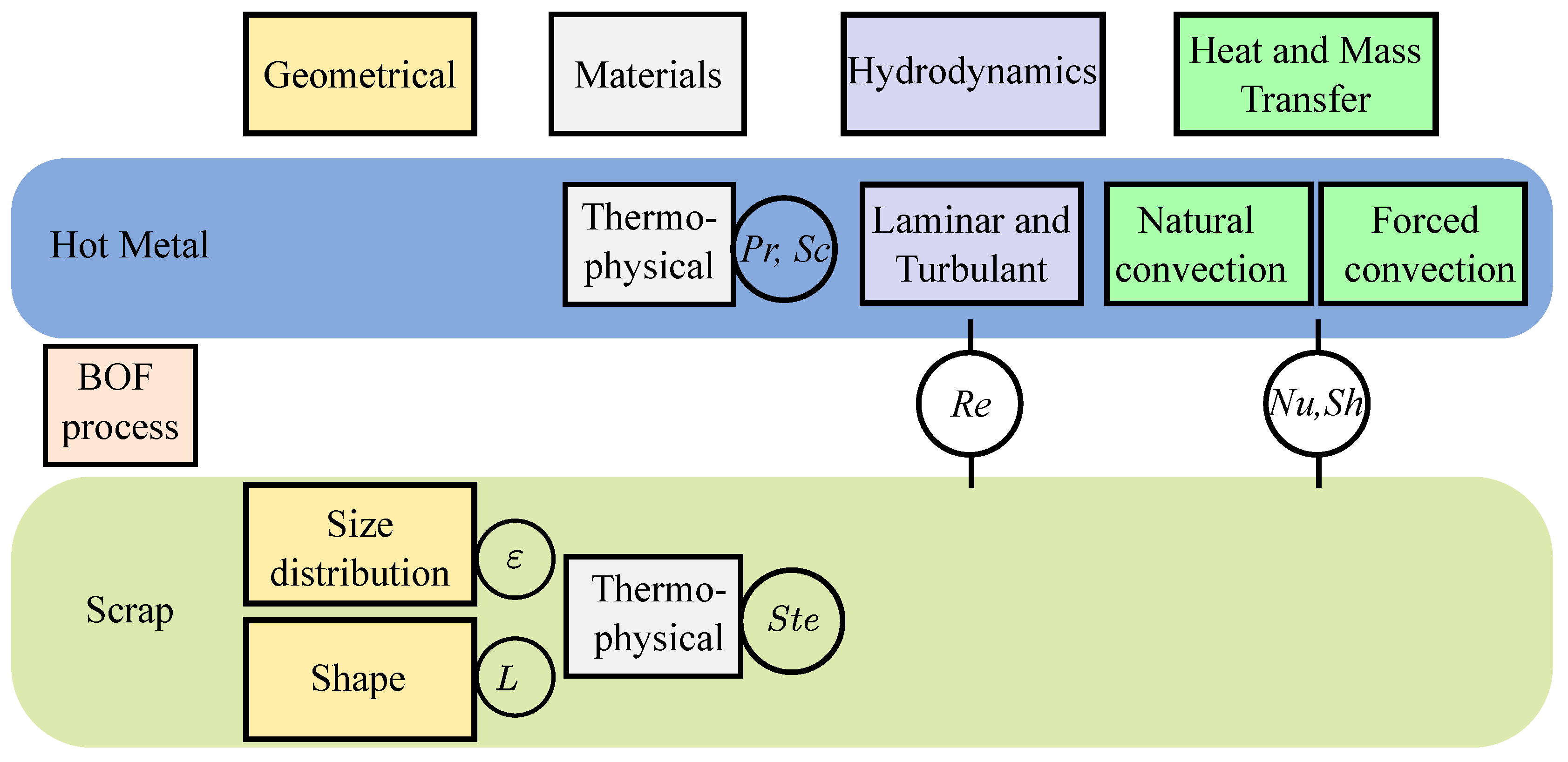
Figure 2.
Normalized particle radius of (initial radius and initial temperature 25 oC ) a single sphere showing shell formation in the quiescent melt of temperature . line a) constant thermophysical properties and heat transfer coefficient, line b) constant thermophysical properties and varying heat transfer as function of the radius, line c) varying thermophysical properties and heat transfer coefficient (Adapted from [38]).
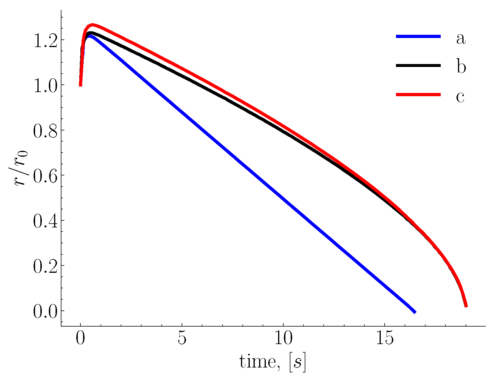
Figure 3.
Mass based normalized melting profiles of (a) the round and, (b) the square steel bars both at initial temperature of and at different melt temperatures (Adapted from [46]).
Figure 3.
Mass based normalized melting profiles of (a) the round and, (b) the square steel bars both at initial temperature of and at different melt temperatures (Adapted from [46]).
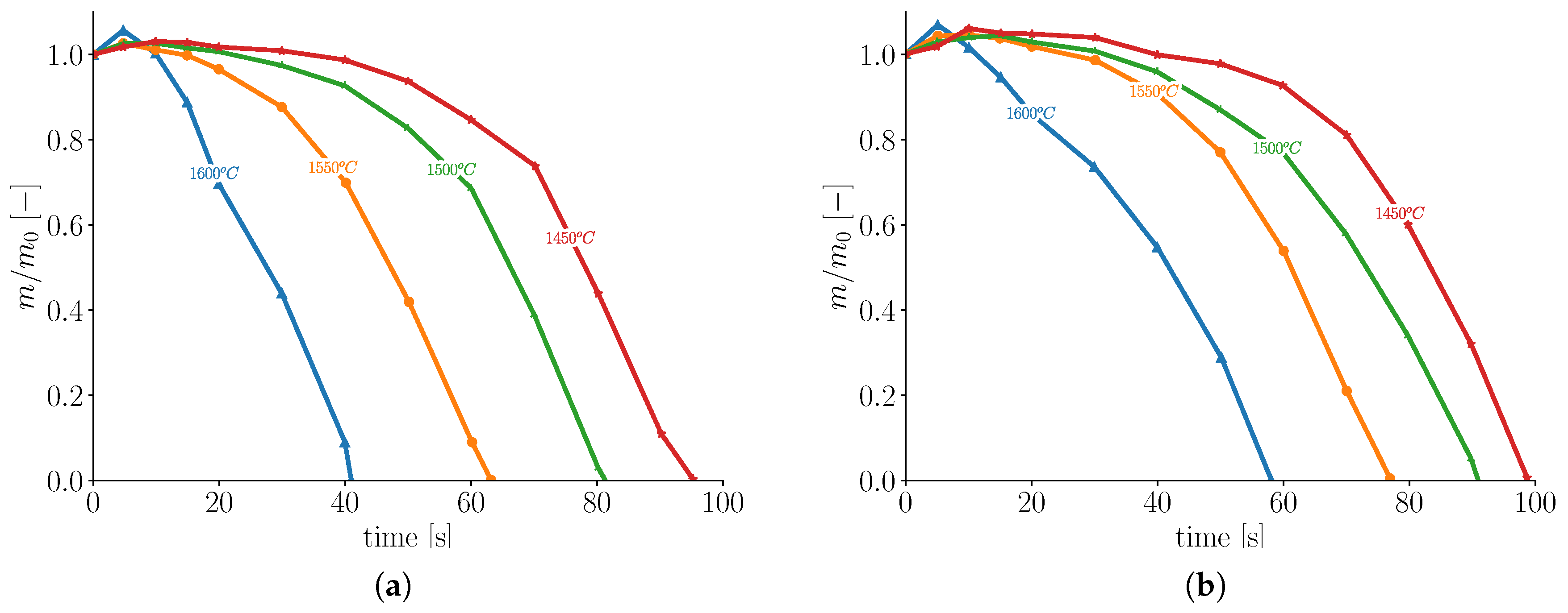
Figure 4.
(a) Radius based normalized rod melting profiles under the influence of natural convection for different temperatures with an initial radius , and a carbon concentration of (Adapted from [12,49]), (b) ablation of steel rods under natural convection melting at different immersion times (colored in red) with bath carbon concentration approximately [50].
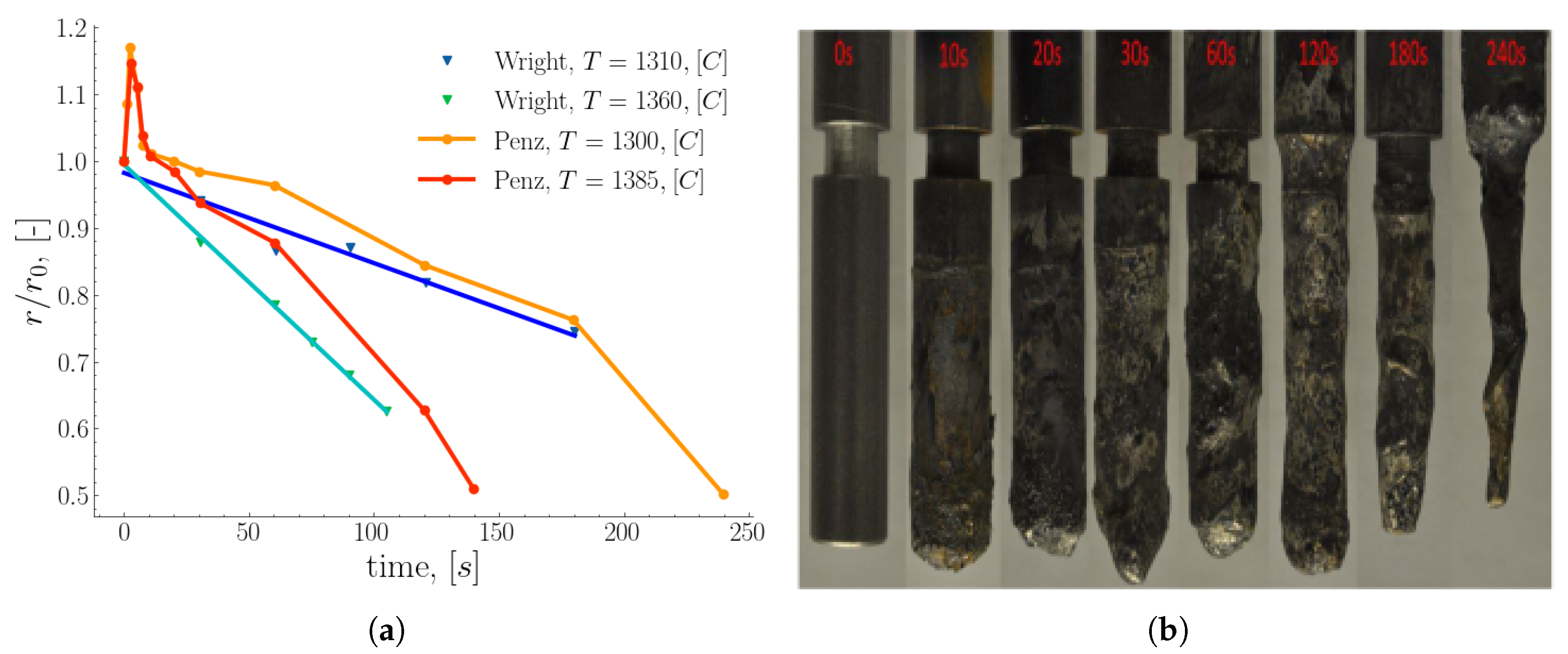
Figure 5.
Comparison of Nusselt correlations for a single sphere as a function of the Reynolds number in the forced convection regime between (a) Argyropoulos et al. [16], (b) Sideman, and (c) Hsu correlations. The circles and the triangles represent the experimental data of the steel and aluminum data, respectively.
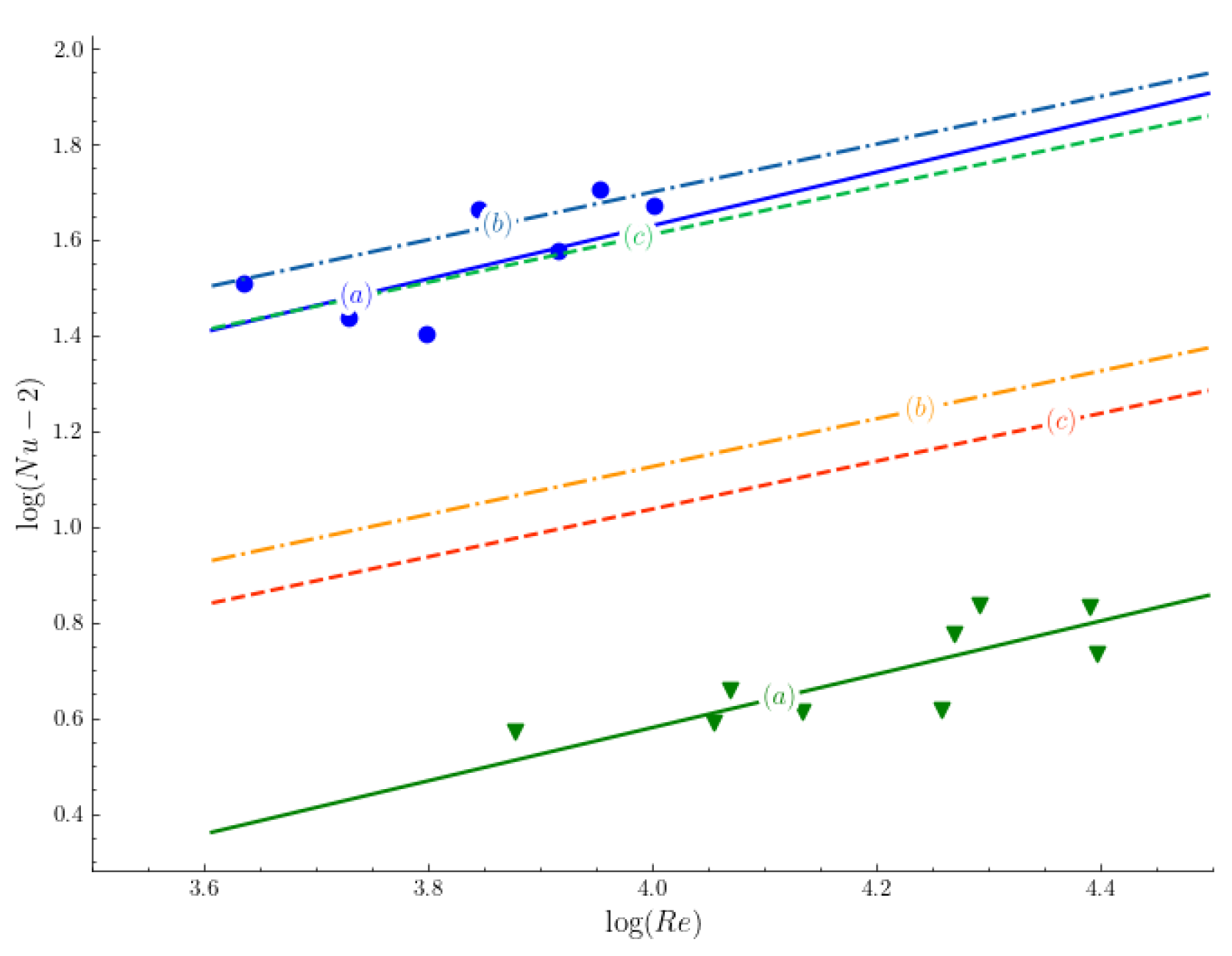
Figure 8.
(a) Modeling the melting of randomly distributed scrap using the phase-field method colored by temperature (Adapted from [6], Copyright 2008 The Minerals, Metals & Materials Society and ASM International. Used with permission). (b) time evolution of particle using (VOF), particles are colored by the volume fraction (1 for liquid and 0 for solid) (Adapted form [82], copyright YEAR, with kind permission from JOURNAL).
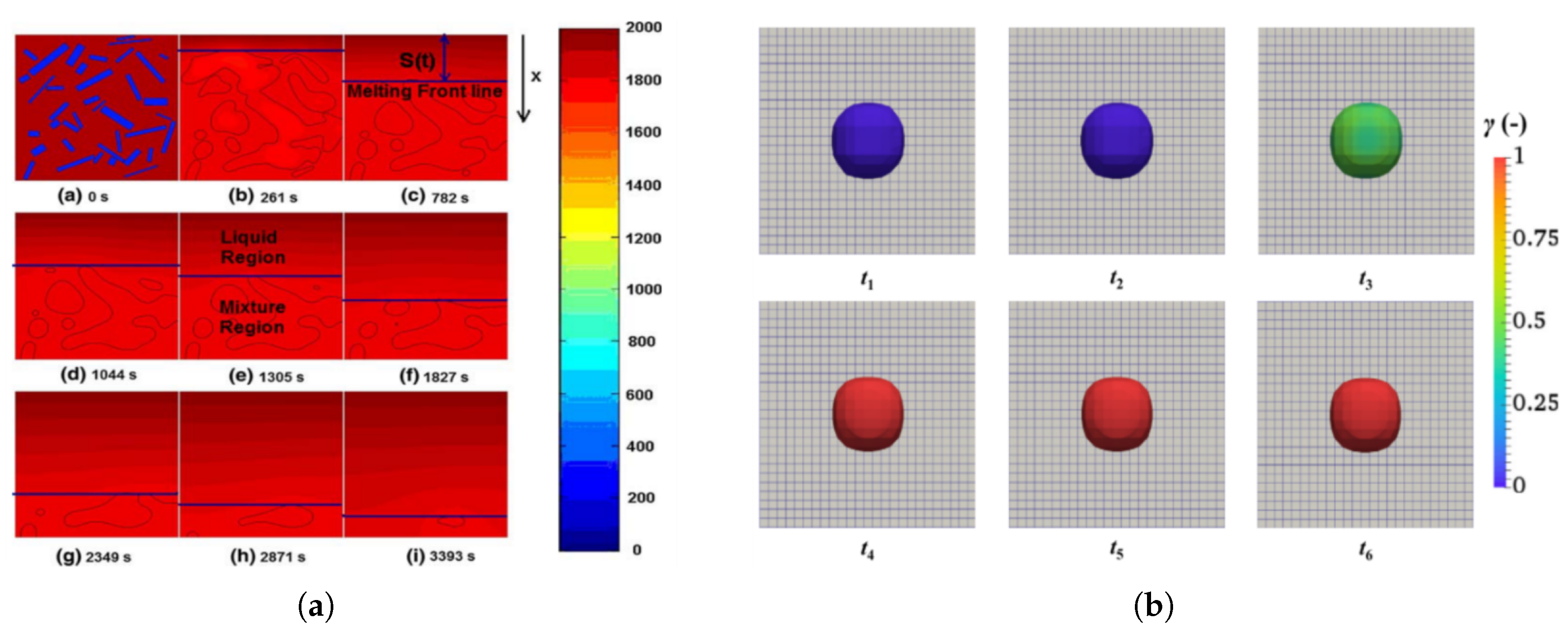
Figure 9.
(a) Non-dimensional temperature distribution of randomly packed sphero-cylinder particles (Adapted from [97], copyright 2015, with kind permission from Elsevier). (b) mean Nusselt number in randomly packed sphero-cylinder obtained from modified Gunn correlation and numerical simulations using cylinder diameter, DNS results are shown by circles, squares, and triangle with different aspect ratio (Adapted from [97], copyright 2015, with kind permission from Elsevier).
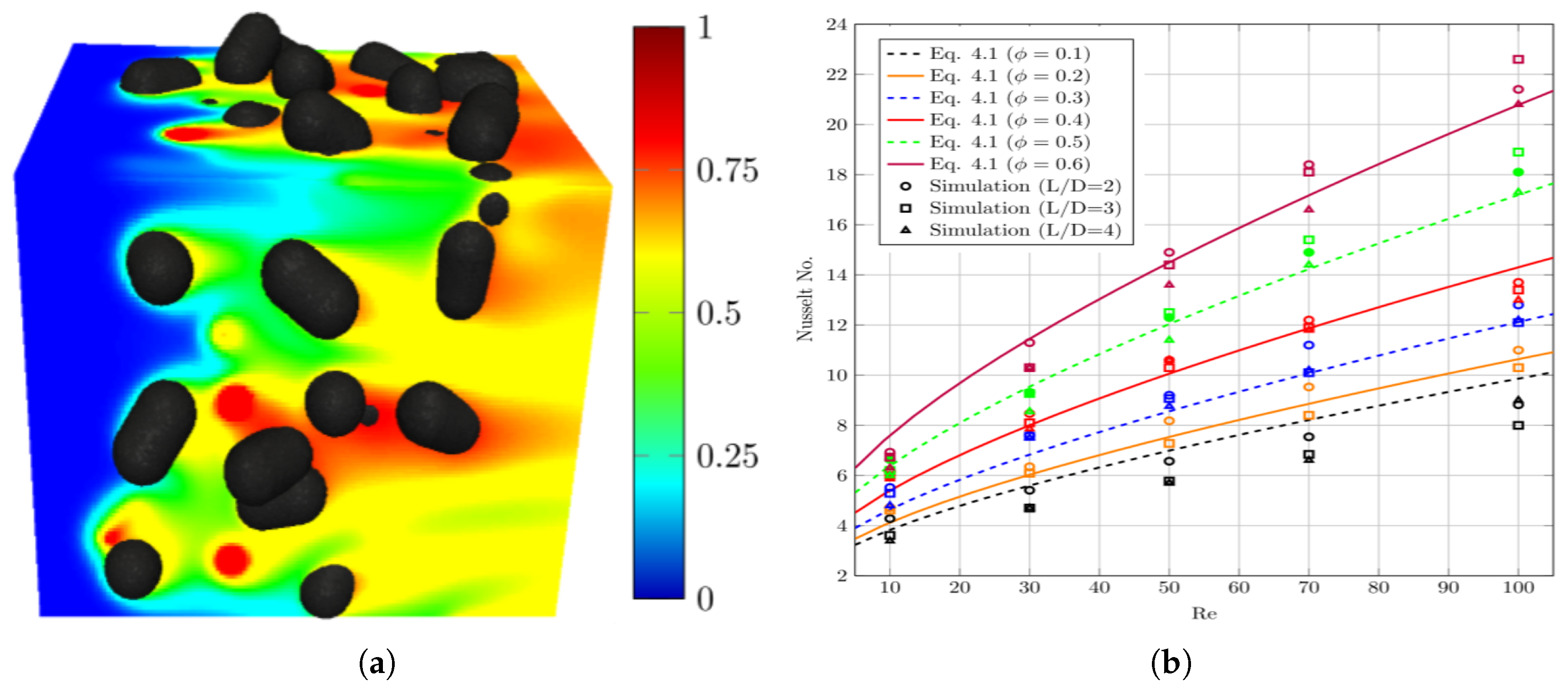
Disclaimer/Publisher’s Note: The statements, opinions and data contained in all publications are solely those of the individual author(s) and contributor(s) and not of MDPI and/or the editor(s). MDPI and/or the editor(s) disclaim responsibility for any injury to people or property resulting from any ideas, methods, instructions or products referred to in the content. |
© 2025 by the authors. Licensee MDPI, Basel, Switzerland. This article is an open access article distributed under the terms and conditions of the Creative Commons Attribution (CC BY) license (http://creativecommons.org/licenses/by/4.0/).
Copyright: This open access article is published under a Creative Commons CC BY 4.0 license, which permit the free download, distribution, and reuse, provided that the author and preprint are cited in any reuse.


