Submitted:
02 February 2026
Posted:
03 February 2026
You are already at the latest version
Abstract
The action principle, long a trusted guide for physicists, now appears to be leading them into dead ends. The reason for this is conjectured to be its inability to properly represent scale covariant physics. The ‘large’ and the ‘small’ are delimited by the size of a physicist, who describes the two regimes using distinct and incompatible languages. An alternative to the action principle is proposed, rectifying this relic of anthropocentric bias by postulating that physicists could exist at any scale, all on equal footing. The consistency between their descriptions of physical phenomena severely restricts the set of their possible observations. So much so that the set of well-behaved, scale-dependent and compatible fields, φ(x, λ), representing spacetime phenomena at any scale, λ, could replace the set of fields which are local extrema of an action, in its role as a “physical law". Observations deemed inexplicable or bizarre when analyzed at any given scale become inevitable when viewed as mere constant-scale sections, φ(x, λ = const), of such scale-orbits. Among them: Why particles rather than a continuum, and why must they not be represented by mathematical points? Why Einsteinian/Newtonian gravity seem to break down at small accelerations? What is the origin of quantum nonlocality? Quantitative agreement with observations is demonstrated in simple cases while in more complicated cases exact routes to testable predictions are shown.
Keywords:
mathematical modeling
; missing mass problem
; quantum foundations
; multiscale phenomena
1. Introduction
This paper is about physics, an essential part of which is the activity of knowledge exchange among physicists, at different locations, different eras, different orientations, etc. The Lagrangian formalism, also referred to as the (extremum-) action principle, is one of several equivalent tools designed to achieve the common ground necessary for such social activity. Physicist A, (mathematically) representing a studied system by , is guaranteed that could (in principle) appear in physicist B’s notes if they use a common action to generate the set of their permissible ’s. To facilitate communication between any two physicists there must also exist a consistent set of dictionaries, translating , which is elegantly provided by the symmetry group of the action. The central role of the Poincaré group in this regard stems from the fact that it provides a necessary and sufficient set of such dictionaries for the vast majority of physicists ever registered. In this paper we ask: Why not extend our Poincaré community of physicists also to include physicists of arbitrary scale?
A cynical reviewer might at this point recommend that this manuscript be resubmitted to a scaled journal, for which there are two good replies. First, to this very day the social activity of physicists is limited to the firm ground of planet Earth and at small relative velocities. Yet the mere act of imagining the existence of physicists anywhere else and at large velocities relative to us is what brought us so far, rescuing physics multiple times from long periods of stagnation. Rejecting even the possibility that physicists could have a size other than that of a physics professor, would be a blatant repetition of the original sin of anthropocentrism. So why not imagine a giant observer for whom our galaxy, or even the entire universe is a mere speck of dust? Or miniature ones, experiencing the creation and subsequent annihilation of a short-lived subatomic particle over multiple generations?—which leads to the second reply: We currently don’t know how to identify a scaled physicist. The cynic might object that we do: Just take all the dynamical fields, , and scale them according to
for some -specific scaling exponent (its inverse `length dimension’); that’s the only way to preserve the multiplicative group property,
he would argue. This implies that scaled physicists comprise scaled hydrogen atoms, which are seen nowhere. Moreover, scaling (1) without alteration of the constants of nature requires physics to be scale covariant, which it isn’t according to our best understanding.
A detailed model addressing the cynic’s concerns has previously been proposed by the author. It accepts the premise (1) hence also the conventional action principle which was never meant to be invariant under (1). There is only a handful of nontrivial scale invariant actions, none of which come close to being realistic. Attempting realism therefore required a very unorthodox application of the action principle manifesting in various technical subtleties, which is never a good sign. However, this is not the main motivation for the current paper. Rather, the form (1) of a scale transformation is too simplistic for a couple of reasons: First, it is only one part of what occurs when, e.g., zooming out of a picture, the other part being a coarsening/smoothing operator. Such coarsening is familiar from the Renormalization Group formalism where is assumed to be a scale-dependent effective representation of some fundamental underlying reality. However, since we can’t allow such assignment of ontological privilege to any particular scale, are equally fundamental irrespective of their . Second, even standalone, (1) presupposes too much about . The Hubble expansion, for example, can formally be viewed as a scale transformation satisfying (2), with the cosmological time playing the role of (the log of-) , but not conforming with (1), in which different structures scale differently depending on their `’. Moreover, (1) doesn’t admit a generally covariant extension, which is a prerequisite for any realistic theory. As (1) results from integrating infinitesimal `naive’ scale transformations
a more flexible rescaling would ensue from substituting (generalizing to a Lie derivative along Z for tensors) where Z is a -dependent scaling field determined on consistency grounds. The -term could likewise locally depend on Z. Combined with some -independent, local coarsening operator , (1) is replaced with
Prescription (3) for scale transformations respects the group property (2), as is easily seen by changing the scale variable to , , in which case (3) becomes
and (2) becomes the group property of a flow. Above and throughout the paper stands for whenever the logarithmic scale s is involved, which should be clear from the context. Crucially, while the effect of , as that of its RG counterpart, is to smooth (equivalently, attenuate its high frequencies) it must not result in a projection, or else scale-flow would be possible only in the forward, viz. direction, with some as initial condition, implicitly privileging the scale .1 Nonetheless, since is a coarsener, flowing backwards in scale typically leads to a singularity, often at finite-s, as the high frequencies grow without bound. It further turns out that compatibility with Lorentz transformations creates a similar problem also in the direction. In the proposed formalism, the tiny subset of solutions of (3) which are well-behaved at any scale, included, and any x, denoted by , plays the role of the set of all extrema of an action.
The set is determined solely by the form of in (3). In other words, given a definition of what a scale transformation is, the mere requirement of consistency between the descriptions of physical phenomena at any scale is what defines the laws of physics. Thus each member of , referred to as a scale orbit, consists of infinitely many fixed-scale sections, each corresponding to distinct yet compatible representations of spacetime phenomena at different scales. It should therefore not come as a surprise that analyzing an individual section not in the context of its full orbit could lead to `bizarre physics’. Critically, unlike in the RG formalism, the scale, s, is not a resolution parameter an experimenter can always control by changing the equipment with which he observes a system, but rather his native scale, encapsulating the totality of instruments and materials he uses when arriving at measurement results. The native scale is an identifier facilitating the dictionary between distinct-scale physicists. A dwarf and a giant can determine whether they are studying the same system, i.e., whether their sections are taken from a common orbit, by propagating in scale their sections at their native scale, to the native scale of the other. Note that by s-translation invariance of (4) one’s native scale is only defined up to a communal constant, i.e. only relative scales matter. Thus a spacetime phenomenon (section) which we, humans, regard as being in the realm of condensed matter physics, a dwarf might label “astrophysical", and so would be his attitude towards us, when slicing the orbit on which we reside at . However, when slicing his orbit at he must arrive at a self-representation which is isomorphic to ours, i.e., , or else we would not belong to the same community of physicists. (Such a distinction between the representations of one’s self and of others, exists also in action based theories, perhaps the most radical example being a physicist boosted to near light-speed becoming nearly two dimensional). The s-translation invariance of (4) then implies with .
Irrespective of its philosophical foundations, the proposed formalism could be used as a phenomenological tool for modeling physical phenomena, no more arbitrary than PDEs and the likes, with multi-scale phenomena, e.g., turbulent flow, being the most natural candidates. However in this paper the main focus is on a model leaning towards the `fundamental’. Although special emphasis is put on gravity, there is no escape from touching other fields, pertaining to the nature of matter and `radiation’, as the proposed model cannot borrow the representation of those from standard theories; it must be able to represent matter, and light needed to observe it, internally (and hopefully more consistently). Obviously, no single paper and no single brain can cover the full breadth of relevant topics. On the other hand, with such panoramic view of physics through a new lens, albeit of low resolution, multiple aspects of the proposed formalism can be explored, enabling novel approaches to longstanding open problems in physics, which are not even expressible in standard language. Finally, to remain at a reasonable length the paper begins with a simple toy model introducing some of the central concepts of the formalism. With that background the reader should be able to fill in certain gaps in the subsequent derivations.
2. Exactly Solvable Linear Toy Model
In order for the notion of native scale to be fully meaningful, must be rich enough to be able to describe: the system being observed; the observer—his equipment included; electromagnetic phenomena involved in most observations, etc. This ambitious task is deferred to Section 3. A gentle introduction to the jargon and techniques used in that section is provided by the flow (4) of a time-independent scalar field in Euclidean D-dimensional space. In choosing the generator of coarsening, , the following properties should be included:
- 1.
- Averaging. If is a local maximum (minimum) then ( resp.)
- 2.
- Locality. is second order and does not contain higher order derivatives or powers higher than the first of the second derivative.
- 3.
- Equivariance. must commute with translations, rotations and reflections in .
The simplest satisfying the above is the (D-dimensional) Laplacian, corresponding to the (weighted) arithmetic average of in the neighborhood of a point. There are, of course, other choices corresponding to different averages2 such as: for a monotonically increasing f, or for any g and combinations thereof (∇ and · are both D-dimensional). The locality clause is a corollary of averaging. Indeed, in 1-dimension for simplicity, a term added to the Laplacian would increase a local maximum of at for , as would an added do to for . However, when takes values in spaces lacking a clear-cut definition of local extremum, locality becomes an independent clause, defining the local, infinitesimal neighborhood of a point. Clause 3 is obviously needed due to the arbitrariness in positioning and orienting one’s coordinate system. Equivalently, it is what defines the community of physicists in Euclidean space.
Sticking with the Laplacian, and using —the simplest scaling field respecting translation invariance of , namely —(4) becomes
with some parameter. It is tempting to attribute a `physical dimension of length’ to , balancing the double derivative it multiplies. However, being a description of physics on all scales, the proposed formalism is inexorably an attempted `theory of everything’ and as such ought to be able to represent any measurement process. And since the result of any measurement is ultimately a dimensionless number, e.g., the number pointed at by a pointer, or the minimal number of standard-length rods exactly fitting a line segment, the notion of physical dimensions should ultimately be abolished. Moreover, since (5) describes a flow in scale, endowing with a dimension of length may lead to the wrong expectation that it too would flow in scale. Nonetheless, the developmental stage of the proposed theory is currently insufficient to internally represent any measurement. To make contact with empirical data associated with sections at our native scale, arbitrarily assigned the value or , dimensions will occasionally appear in this paper. Unless stated otherwise, is assumed, i.e., the coordinate x at is measured in multiples of . Note that even this innocuous statement relies on the existence of an affine structure of space whose physical validation requires an affine structure of space! Thus without doing away with this circularity via a general covariant extension of (5) (Section 3), our proposal cannot even pretend to be a fundamental physical theory.
2.1. The Particle Basis of
Of special interest are fixed-point solutions of the flow (5), i.e., scale-invariant , of which fixed-points which are further global or local attractors stand out. To find the latter we note that, if is integrable at —the case of a non-integrable is dealt with later—its zeroth moment, , satisfies and explodes for , implying , unless and without loss of generality by the linearity of (5), or else . Assuming the former for now, it is helpful to represent by its cumulants. Taking the Fourier transform of (5) and dividing by the Fourier transform , which is also the generating function of its moments assumed all to exist, leads to the following equation for the generating function of the cumulants,
Equation (6) is an infinite set of uncoupled ODEs for the coefficients, , of multinomials whose solutions all vanish for except those of which approach . Solving back, , we get the Gaussian
which is therefore a global attractor of the flow (5) for (moment-determinate) functions with well defined moments to any order at . However, not all moment determinate are sections of orbits in . A large subset that is, consists of linear combinations, discrete or continuous, of shifted fixed-point Gaussians. This is so because any such sum has well defined moments to any order and the effect of the flow on individual Gaussians is a trivial shift
We strongly suspect that the converse is also true, namely, that any can be decomposed into a linear combination of shifting Gaussians. A formal proof will not be attempted here but the intuition must be clear: The Laplacian increases (decreases) and `sharpens’ at its local maximum (resp. minimum) when flowing in the direction of (5), and if the scaling part does not sufficiently compensate for this, wildly diverges at a local extremum. Any section of must therefore be `round’ enough on the scale set by () and if so it should be decomposable into Gaussians of width . A clear illustration of the fate of a function not sufficiently round is provided by a Gaussian of width less than 1 at , i.e., . A finite-s singularity is reached at where vanishes, corresponding to which is a `delta-function Gaussian’.
Closure under continuous sums is what distinguishes the shifted Gaussians basis of , referred to as the `particle basis’, from the scaled Fourier basis,
Although individually in , infinite sums thereof may still lie outside , as the above narrow-Gaussian example demonstrates. Nonetheless, the pseudo basis (8) is not entirely useless. It clearly shows the rapid decay of waves when their wave-vector is contracted beyond the cutoff frequency () and will serve us in the sequel.
Returning to the case of non-integrable, or integrable but zero , the corresponding fixed-points of (5) are in for a suitable , , vanishing at , which happen to have a asymptotic tail hence are non-integrable. It can be shown that the basin of attraction of each consists only of itself, rendering it uninteresting from our perspective.
Full justification for the name “particle" attached to Gaussians of width and -moment equal to 1 (or any other normalization) will have to await Section 3 but some can already be given at this stage. If physicists of different native scales are to have isomorphic self-representations—their laboratory etc. included—and if physicists exist at arbitrarily large or small scales (but not necessarily at any scale) then they must all consist of the same particles and their `oppositely charged’ antiparticles—Gaussians of width and -moment . Otherwise particle-antiparticle pairs would not get fully annihilated when flowing via (7) in the direction. As a result, the `vacuum’ would get increasingly contaminated with particles of arbitrary charge. Conversely, the vacuum could only acquire content when zooming into an empty patch of it, if particle-antiparticle pairs are created out of it. Note that the decomposablility of into a discrete sum of particles is required by the fact that would otherwise trivialize to a uniform for . Thus our model requires for its consistency both particles and the quantization of their charge. Moreover, in the point-particle limit, , it would take for any pair to annihilate even approximately, contradicting the existence of scaled physicists. Point-particles, which are the source of all evil in mathematical physics, are excluded from the outset.
2.2. Adding Time Dependence
How should the flow (5) be generalized for a time-dependent ? Guided by the equivariance clause with the Poincaré group replacing the isometry group of Euclidean space, the unique generalization reads
The coefficient multiplying is assumed to equal 1 unless stated otherwise. In covariant notations, (9) reads
with and . Readers experiencing unease from the appearance of Lorentz symmetry out of the blue are referred to [4]. It has been known since the early years of Relativity Theory that Lorentz transformations were only serendipitously discovered within the framework of electrodynamics. This symmetry group (the Galilean group being a limiting case thereof) is an inevitability when the meaning of synchronized clocks is logically analyzed—which is essentially what is being done in this paper with regard to scale transformations. Thus our proposed time-dependent generalization of inexorably involves values of at times other than t, but not because space and time form a `spacetime’ continuum—the Minkowskian/geometric view (if that were the case then would be expected to have the opposite sign). Instead, space and time are fundamentally distinct and are mixed together on consistency grounds; without such mixing no community of physicists would exist.
Generalizations of static particles are—naturally—moving particles and in particular uniformly so, obtained by boosting a static particle solution. In for simplicity, the boost explicitly reads with , making the Lorentz contraction of the particle in the direction of motion manifest. Uniformly moving particles are therefore all members of , but are all members of such? More accurately: Do they form a basis for ? To answer this question, (9) is first integrated over three-space. Assuming the integral exists, this results in the following equation for the zeroth moment
Plugging a scaled Fourier ansatz and continuing with the case, we get: implying or else it explodes for . For , is some constant which can be assumed to equal 1 by the linearity of (9). We conclude that which is constant in both time and scale is a necessary condition for the corresponding to lie in . Next, consider the generalization of equation (6) for the time-dependent cumulants of ,
similarly obtained by Fourier transforming (9) and dividing by . Using (12) we first argue that the instability of the flow (9) in the direction, which mandates particles, in and of itself does not further mandates their uniform motion. To show this we plug the following ansatz into (12), continuing with for clarity
where is a double-indexed function of the scaled time alone. Equating the coefficient of each power of k to zero in increasing powers of (note that the series is missing the term by our result ). Starting with , dictating the asymptotic scaling form of the center-of-mass, i.e. , we see that it decouples from all other terms in the limit and can be an arbitrary function. Successive terms, , can then be iteratively computed as the term does not contain the first power of k, and the term pulls out an extra factor of , e.g., (all evaluated at the scaled time ). For with bounded time derivatives to all orders, the power series of clearly converges for . Moving to , the leading order of (minus the-) variance reads with again manifesting the Lorentz contraction. Higher order corrections, , can then be calculated in terms of and products , coming from the nonlinear term, e.g., . The leading order term of the third cumulant, the so called “skewness", reads . It is likewise a relativistic effect in which the `front’ and `back’ of an accelerating (extended) particle experience different Lorentz contractions. Continuing this way, can be computed in terms of and its first derivatives. The results in a convergent power series for each at . As , at small enough scale the shape of a particle is approximated arbitrarily well by that of a uniformly moving particle (appropriately Lorentz contracted in the direction of motion). The leading order correction appear in the form of a particle’s skewness in the direction of acceleration (predicated on relativistic velocities). We conclude that a sufficient condition for to well-behave at small scales is that it approaches a sum of scaling particle solutions, generalizing the static-particle result. Although more difficult to prove, there is no apparent reason why this conclusion should not carry to nonlinear scale-flows in the case of a single particle.
Returning to our original question, of whether necessarily describes a uniformly moving particle, we turn to the fate of such a well localized moving particle solution at small , entirely encoded in the single function , when it flows to large , outside the convergence radius of the each cumulant’s power series. We prove that the answer is positive, viz., unless describes a globally freely moving particles, for some and v, its corresponding is not in . This is due to a new flow instability in the direction, introduced by the minus sign of the term in (9). To prove this, consider the equation for the center of the particle (switching notations in order to not overload the upper index)
obtained by equating the coefficients of in (12) to zero (i not a power!). Now plug into (14) the most general solution
with the sum representing also an integral, and the ’s are the Fourier coefficients of . Clearly, unless , and insofar as still describes a localized particle, this particle (wildly) moves around unbounded for which in and of itself implies ; any `wrinkle’ in a straight path at gets rapidly amplified at large by the term in (14). However, moving to higher order cumulants, which are all morphological attributes of a particle-like hence independent of , a similar divergence occurs, implying either the divergence or its complete delocalization.
Another way of seeing why only uniformly moving particles appear in is by decomposing a non-uniformly moving particle solution at into its space-time Fourier components, and letting them each flow to . Their evolution in scale is just (8) with meaning (and ). Waves with are strongly attenuated at large , while those with blow-up. Now, it is easily verified that any non-uniform, or uniform but superluminal motion at , must have some time-like () Fourier components in its decomposition, expelling the orbit on which it resides from . This method is applicable also to possible superpositions of non-uniformly moving particles having for their joint . Rather than resorting to murky causal paradoxes, or to our current inability to accelerate masses beyond the speed of light, the proposed formalism rejects Tachyons on simple mathematical grounds. The dominance of waves with light-like k’s can also be appreciated even before moving to more complicated models.
3. A Realistic Model
The alert reader must have anticipated the main result of the previous section, namely, that consists of freely moving particles. By linearity, particles can move through one another uninterrupted and if so, they are noninteracting particles which should better have straight paths. Enabling their mutual interaction therefore requires some form of nonlinearity, either in the coarsener, , or in the scaling part. Further recalling our commitment to general covariance as a precondition for any fundamental physical theory, nonlinearity is inevitably and, in a sense, uniquely forced upon us. A nonlinear model also supports a plurality of particles, having different sizes which are different from the common in a linear theory. This frees , ultimately estimated at km, to play a role at astrophysical scales.
Our realistic model involves a spin-1, field: The A-field. A straightforward (and unique up to terms involving the curvature) way to render a differential operator generally covariant is through the minimal-coupling prescription, of `dotting the commas’ which can be applied to the `Maxwell coarsener’ . The scaling piece of an covariant vector is just its Lie derivative with respect to the scaling field, , defined below. Combined, the scale flow of reads
with
the Lie derivative of with respect to . In flat spacetime and , (17) reduces to `naive’ scaling, . Equation (16) prescribes the generally covariant scale-flow of a vector in one particular coordinate system common to all scales. Thus is partitioned into equivalence classes, the members of each are related by some coordinate transformation.
Fixed-points of the flow (16), which are therefore members in , are all solutions of Maxwell’s equations sourced by the peculiar current . Once is defined it will transpire that this current is localized around world-lines where peaks, providing a detailed microscopic description of the structure of matter. However, is clearly much larger than the set of such solutions and, as in the linear model, its building blocks are (fixed-point) particles. Direct analysis of particles in space is much more difficult than in the linear, case, as no moment of the associated particle exists due to its non-integrable Coulomb tail. To facilitate the analysis of such extended particles, we define a auxiliary model for the center(oid) of
(which for a fixed point equals ). Continuing in a standard way by operating with on (18) using the antisymmetry of , the commutators of covariant derivatives
and the symmetries of the Riemann tensor, gives , i.e., is covariantly conserved at any scale, s. Above and throughout the paper Weinberg’s sign convention for the Riemann tensor is used
Operating on (16) with (recalling that ) the second term of this operator almost annihilates the coarsener by the above remarks (charge conservation), leaving only a curvature term coming from commutator (19). The scaling piece is evaluated using the commutativity: for any 1-form A, which gives , leading to the desired conversion (see Section 3.2 below). The l.h.s. reads . We would like to swap the order of and , which would give by (18). However, in curved spacetime could implicitly depend on the scale s through , introducing a gauge invariant (albeit not manifestly so) commutator correction. The combined result reads
more suited for analysis. It is emphasized that and its associated scale flow are merely analytic tools, not to be put on equal footing with and its flow. As the nonlinear terms arising from scaling and commutator do not involve but rather , for a given and , (21) describes the linear but inhomogeneous—in both spacetime and scale—flow of .
Relation (18) is formally equivalent to Maxwell’s equations with sourcing ’s wave equation. However, is not an independent object as in classical electrodynamics but a marker of the locus of privileged points at which the Maxwell coarsener does not annihilate ; distinct ’s differing by some therefore have identical ’s. And just like in the scalar-particle case, where higher order cumulants () are `awakened’ by its center’s nonuniform motion, deforming its stationary shape, so does the “adjunct" (in the jargon of action-at-a-distance electrodynamics) to each such gets deformed. Due to the extended nature of an A-particle, and unlike in models3, these deformations at are not encoded in the local motion of its center at time t, but rather on its motion at retarded and advanced times, (assuming flat spacetime for simplicity). However, associating such temporal incongruity with `radiation’ can be misleading, as it normally implies the freedom to add any homogeneous solution of Maxwell’s equations to which is clearly nonsensical from our perspective. Consequently, the retarded solution cannot be imposed on and in general, contains a mixture of both advanced and retarded parts, which varies across spacetime. The so-called radiation arrow of time manifested in every macroscopic phenomenon must therefore receive an alternative explanation (see Section 3.5.2).
Summarizing: As already seen in the linear, time-dependent case, a scale-flow such as (16) suffers from instability in both s-directions; Local variations of along space-like/time-like directions which are not almost annihilated by the (second order) coarsener, W, get rapidly amplified in the / direction resp. The scaling piece, being only first order, can only counter this rapid amplification inside the support of —which for a fixed-point equals —where the scaling field, , peaks, i.e., inside matter (Section 3.1.2 below). “Almost" is emphasized above because, for non fixed-point members of , the coarsener does not fully annihilate outside , only reducing it to the order of the scaling piece’s action, giving rise to deviations from classical physics. This will be a recurrent theme in the rest of the paper.
3.1. Determining the Metric and the Scaling Field
The flow (16) of requires specifying both and in a generally covariant way. Starting with the former, we seek the scale flow of . It is well known that, in Riemannian geometry, the Ricci tensor is the unique, symmetric generally covariant tensor which can be constructed from the metric tensor and its first two derivatives and does not contain higher power than the first of its second derivative. By our definition of a coarsener, this leaves with and , as the only permissible coarsener for some constant b. Now, the flow (16) of is `guided’ by via the minimal coupling prescription. On consistency grounds the flow of must also be guided by , or else the gravitational field would not focus around matter. The simplest way to achieve this mutuality is through the use of the (symmetric) canonical energy-momentum tensor
peaking around and likewise gauge invariant, which leads to the following scale flow of :
with , G and b some constants, and
The global sign of the coarsener piece reflects Weinberg’s sign convention for the Riemann tensor (20).
Taking the covariant divergence of (23), and using (as a result of the Bianchi identity) implies that
is a necessary condition for (23) to have a solution. Defining
equation (25) can be rewritten as
Postulating that energy-momentum conservation is recovered in the limit mandates , nullifying the last term on the r.h.s. of (27), which is assumed henceforth. The possibility that gravity is essentially involved in the structure of elementary matter [5], and consequently is nonphysical, has not been explored. The first, divergence term on the r.h.s. of (27), when properly absorbed into the l.h.s. (see Section 3.4), results in an altered, exactly conserved and more physically meaningful energy-momentum tensor.
Finally, the decision to treat as yet another fundamental field on equal footing with the A-field, rather than as a scale-specific `scaffold field’ like (see next) is not an obvious one. Except in the relativistic cosmological model, solving (23) with the l.h.s. set to zero at each s along the scale flow of , would not make much of a difference. The scale-flow treatment turns out to be an elegant and natural way to enforce this family of s-dependent constraints on .
3.1.1. Determining the Scaling Field
Assuming leads to significant simplification when determining , and is therefore considered first. In this approximation covariant derivatives appear as ordinary derivatives, , and (27) reduces to energy-momentum conservation
Purely by the symmetry and conservation of , generalized angular momentum conservation follows
By virtue of definition (18) of (Maxwell’s equations) and the Maxwell-Bianchi identity () alone, Poynting theorem is satisfied identically
hence (28) implies
Maxwell’s equations (18), along with (29) and (30), referred to henceforth as the basic tenets of classical electrodynamics, are nowadays taken as the definition of classical electrodynamics, encapsulating its experimental success. However, we shall see in Section 3.4 that the usual derivation of the Lorentz force equation from them, which circumvents the infamous unresolved classical self-force problem of point charges, requires a special treatment.
Equations (26) and (30) result in four second order equations for the four components of the scaling field ,
Together with the boundary condition away from matter a (non singular) solution is uniquely defined up to a solution for the homogeneous equation. This last freedom is removed by demanding continuity in .
Summarizing, as a corollary of defining the scale flow of the metric, a definition of the scaling field at each scale was obtained. A generalization of (31) to curved spacetime follows from adding the r.h.s. of (27) (with ) to the r.h.s. of (31),
and using a covariant form for the boundary condition
3.1.2. Time Independent Fixed-Points in Flat Spacetime
Now that depends on via (16), and on via (31), the nonlinear nature of the flow (16) can be appreciated, as well as the indirect mixing of and through , even in the time-independent case; note that in this case, (31) plus b.c. at infinity uniquely define a regular solution at each s. Finding the fixed-points and their basins of attraction for the nonlinear flow (16)(31) in the general, time-independent case, deserves a separate paper(s). As in the linear case, the battle between the dissipative effect of the coarsener and the contracting effect of enforced by its large b.c., implies that propagating some initial, time-independent and to large s always leads to a fixed-point. Below we directly solve the fixed-point equations for a charged, spherically symmetric, non-spinning () case in order to demonstrate how the nonlinearity introduces a second length scale, governing particle physics, which unlike is an attribute of the solution rather than a parameter of the model. The physical relevance of this fixed-point is questionable as its basin of attraction might consists only of non-spinning ’s.
For , , the r.h.s. of (30) is an outwards-pointing radial force with
Plugging
into (31) with boundary conditions , (for the Laplacian to be well-defined at the origin) and translates into and a second order ODE for
Setting in (16) gives
The system (35)(36) is symmetric under , , guaranteeing that fixed-points come in particle-antiparticle pairs, which is true also in the general case. Since , the system is under-determined, i.e., its solutions involve four integration constants satisfying only three independent conditions, therefore specifying a one-parameter family of solutions. Solutions of (35) are
A particle solution is defined by , hence also , for , where is the particle’s radius (`matter’). Inside matter , implying .
Using , obtained from the analytic solution near , the system (35)(36) can be numerically integrated from using as a free parameter, adjusting to meet , with the result that monotonically and unboundedly decreases with increasing .
The Poincaré stress-energy tensor (26) reads
consisting of a z-independent `vacuum energy-momentum’ piece, , entirely due to the boundary condition (33), and a z-dependent, particle-specific `matter piece’, , which is colocalized with . The trace of is positive inside matter; Poincaré would have interpreted this as the negative pressure holding the particle against its internal Coulomb repulsion, and the nontrivial scaling field, , as the displacement vector due to the Coulomb stress. Since the positive `Coulomb pressure’ inside a charged particle is on the order of , equilibrium with the Poincaré pressure mandates a huge for and a typical subatomic scale, e.g., the classical electron radius or the proton’s radius; Remarkably, all attributes of a particle involve gravitational parameters, G, and . Asymptotically, . The component vanishes, thus the particle’s energy is attributable entirely to its electrostatic self-energy .
In conclusion of this section, a few final remarks. First, the above particle solution, although involving a nonlinearity, must not be conflated with soliton solutions of nonlinear PDEs, having a long history in modeling of particles. The existence of particles in the proposed formalism does not hinge on the flow being nonlinear (as seen in Section 2), but rather on a unique scaling operation countering the coarsener, therefore requiring a large scaling field inside a small particle. Second, charge quantization could be explained by cosmological considerations, of the type discussed at the end of Section 2.1. As in the linear case, and as seen in the spherically symmetric solution, fixed-points depend on a continuous parameter, controlling all their attributes this time, which is `spontaneously’ fixed at its observed value by a global consistency condition. Alternatively, charge quantization may arise just from the fixed-point condition for a spinning particle, where the reduced symmetry of the solution eliminates said free parameter. Finally, some/most/all real-world particles are likely represented by time-dependent solutions, which are fixed-points only in the statistical sense, when averaged over sufficiently long yet microscopic time intervals. Since , the time-averaged energy would vanish nonetheless. The time dependence of such solutions would need to be chaotic, with a scale invariant power spectrum up to some cutoff frequency. Analyzing the properties of such dynamical fixed-points is suited for a statistical theory, complementing the proposed realistic model on such issues, which presumably is quantum mechanics and its generalizations; see Section 3.3
3.1.3. The Gravitational Field of a Matter Lump
Moving one step beyond the flat spacetime approximation, the distortion to and caused by a fixed-point solution is calculated. To this end the flat metric is replaced with a (quasi-)static metric
with non-vanishing Christoffel symbols
and we seek a fixed-point solution of the metric flow (23), with now calculated using (39) instead of , and solving (32). Starting with the latter, the non gravitational part on the r.h.s. of (32), involving , vanishes outside matter and is ignored. The remaining, gravitational equation, has on its r.h.s. a source, which for a fixed-point reads:
for some offset , where is the metric perturbation adjunct to particle/fixed-point p. In the above expression it was assumed that during scale flow, `naive scaling’ alone rigidly shifts the center of an offset fixed-point, which turns out below to be a consistent assumption. Using the metric (39) and an ansatz in (32): , , with , translation invariant equations for are obtained,
with solutions . This component of , adjunct to a body, is the gravitational counterpart of from the previous section. Note that, as with , for multiple fixed-points at close proximity, is not a solution (individual must get deformed for that). However, such departures of from naive scaling only introduce corrections to quantities, and are neglected henceforth.
Next, using (39) for the metric in (23) and temporarily dropping the `p’ label from gives
for the time-time component, with being the metric part of , resulting from in (26)
which contains a vacuum piece (the matter piece, vanishes—see previous section where it was referred to as simply ) and a scaling (or convective) piece. A consistent treatment of the spatial components requires a slightly more general metric ansatz than (39), . However, this would necessitate a accurate to and only result in an correction to . For the sake of clarity this complication is neglected below.
Equation (41) is just the inhomogeneous flow of a scalar which is valid outside matter, and inside it if gravity plays a negligible role in the structure of matter. Choosing an offset we obtain the fixed-point equation for a particle stationed at the origin
At distances from the source smaller than , solutions of (43) are approximately the usual solutions of Newtonian gravity, , with (plus a repulsive, potential at leading order in in the consistent treatment).
The covariant counterpart of (41) is
Generalizing (42) is the following decomposition of :
and complementing it to the full , which by (32) satisfies outside matter
with far away from matter. A solution for (46) has the form
with the radiative part identified by the form of far away from matter (see Section 3.4). Fixed-point solutions of (44) are just solutions of Einstein’s field equation for . The physical meaning of solving (44) is only revealed through its effect on , and in the following sections the reason for this peculiar coefficient of G becomes apparent.
In most realistic scenarios, is time-dependent, focused on the worldline, , of a particle. The flow of the adjunct metric perturbation solving (23) then involves a form more general then (39): , , with also time-dependent, and (23) becomes
where and are the Einstein tensor and linearized around . At distances from much smaller than , the linearized EFE must then be (almost) satisfied for to not rapidly diverge at large , and for a non-relativistic and a sufficiently small sourcing mass, m, the off-diagonal elements of are negligible. The diagonal form of clearly persists to distances greater than , where is negligibly small, and (48) becomes a single equation
with and the negligible term above retained for the pedagogical reason: A solution for a uniformly moving can then be obtained by simply boosting the previous static perturbation as in Section 2.2 (though only to nonrelativistic velocities for consistency).
In Summary, given any collection of nonrelativistic world-lines where `p’ is a particle label
with the Newtonian potential carried by mass , is necessarily the approximate, point-wise form of any, everywhere and at all regular global solution of (49). The role of the scaling terms in (49) is to ensure translation covariance, i.e., the freedom to choose the scaling center at will: If solves (49) with focused on , then so does with for any .
3.2. The Motion of Matter Lumps in a Weak Gravitational Field
Equation (50) prescribes the scale flow of the metric (in the Newtonian approximation), given the a set, , of worldlines associated with matter lumps. To determine this set, an equation for each , given , is obtained in this section. This is done by analyzing the scale flow of the first moment of associated with a general matter lump, using (21). An obstacle to doing so comes from the fact that, now incorporates both gravitational and non gravitational interactions in a convoluted way, as the existence of gravitating matter depends on it being composed of charged matter. In order to isolate the effect of gravity on , we first analyze the motion of a body in the absence of gravity, i.e., , with the Minkowskian coordinates and the structural component from the previous sections. To this end, a better understanding of the scale flow (21) of is needed. Using (17) and (18) plus some algebra the scaling piece in (21) reads
with
The first two terms in (51) are the familiar conversion, to which a `matter vector’, , is added. In the absence of gravity the commutator on the l.h.s. of (21) vanishes. Combined, we get
Note that, since , taking the divergence of (53) necessitates , which is indeed the case by virtue of the antisymmetry of . Defining and the (conserved in time-) electric and `matter’ charges resp., and integrating (53) over three-space implies i.e., electric charge is conserved in scale if and only if the matter charge vanishes. That the latter is identically true follows from the divergence form (52) of and . This result readily generalizes to curved spacetime4 for an s-independent metric, by virtue of the (covariant) divergence of the r.h.s. of (21) vanishing, implying that the charge of a matter-lump is conserved in scale whenever spacetime is approximately s-independent around some point on its world-line; For then where the second implication follows from charge conservation in time. Note that, unlike in the linear model of Section 2, identical charge conservation holds true whether or not corresponds to a member in , but this does not seem to carry to the s-dependent-metric case, which involves the delicately choreographed, regularity preserving scale-flows of both (hence also ) and . However since gravity is assumed to play a negligible role in the stricture of charged matter, such s-dependence is inconsequential to members in . Alternatively, if as in the linear model, zooming into matter must reveal only more and more copies of the same charge-quantized (fixed-point) particles, then the issue of identical charge conservation even for becomes moot.
Next, multiplying (53) by and integrating over a ball, B, containing a body of charge q, results in
where is an object’s `center-of-charge’ (c.o.c.). Above and in the rest of this section, the charge of a body, assumed nonzero for simplicity, is only used as a convenient tracer of matter. As can be both positive and negative, the c.o.c. is not necessarily confined to the support of , as with positive distributions. Nonetheless, since , does follow the particle up to some constant displacement, reflecting to a large extent the arbitrariness in defining the exact position of an extended body, and assumed much smaller than any competing length.
At the (sub-)atomic level, would be rapidly fluctuating in time, endowing with a `jitter motion’ component. To remove it, (54) is convolved with a normalized symmetric kernel of macroscopic extent T. Defining
the form of (54) is retained for (with ), except for a correction
coming from the time-scaling term. If is slowly varying over T, this correction is at most on the order of , negligibly renormalizing the term for . For economical notations, then, the `bar’ is dropped henceforth from all quantities.
The integral in (54) is the first moment of a distribution, , whose zeroth moment vanishes; It is therefore invariant under —as is expected of a `force term’, competing with the , acceleration term. Buried in it are presumably all forms of non gravitational interactions potentially preventing for some constant and , from being a solution of (54) in the absence of gravity. Accordingly, this term is ignored for an isolated body, for which all forces are internal and necessarily integrate to zero (this can be verified explicitly, e.g., for a spherically symmetric ). Since for an isolated fixed-point must be a solution for (53), it is concluded said integral must vanish. Equation (54) then becomes (14), and as proved in that case, solutions for must all be straight, non tachyonic worldlines .
The effect of gravity on those straight worldlines is derived by including a weak field in the flow of the first-moment projection of (21). Recalling from Section 3.1.2 that weak gravity has no effect on the scaling field, and since gravity is assumed to play a negligible role in the structure of matter, the way this field enters the flat spacetime analysis is by `dotting the commas’ in partial derivatives. To this end the Newtonian metric (39) is substituted into (21), which is then multiplied by , where
is the charge of the matter lump, conserved in both time and scale, and integrated over B, assuming is approximately constant over the extent of the lump. A straightforward calculation to first order in , incorporating , gives
Ignoring corrections to the isotropic coarsener, the net effect of the potential in the Newtonian approximation is to render the coarsener anisotropic through its gradient, with an added relativistic correction in the form of the last term on the r.h.s. of (57). At non-relativistic velocities the double time-derivative piece equals , where . The correction turns out at large scale and completely negligible at small, hence ignored. In the second term on the r.h.s. of (57) the cancels the factor multiplying it, which is then integrated by parts. To accuracy the result is . Using the continuity equation for , integration by parts of the last term in (57) yields a relativistic, term, neglected in the Newtonian approximation. The modification to the scaling piece (51) introduces an correction to the term in (54) which is neglected in the Newtonian approximation. Since , the contribution of the curvature term vanishes, as is that of the covariant term by our assumption that the lump would otherwise be freely moving. Moving to the contribution of the two terms on the l.h.s. of (21), the commutator is evaluated using (viz., ordinary derivatives can replace covariant ones) in the definition (18),
To accuracy its first moment projection gives . Combined with the contribution of the term their sum is the expected .
Combining all pieces, the first moment projection of (21) reads
This equation is just (14) with an extra `force-term’ on its r.h.s. which could salvage a non uniformly moving solution, , from the catastrophic fate at suffered by its linear counterpart.
At sufficiently large scales, , when all relevant masses contributing to occupy a small ball of radius centered at the origin of scaling without loss of generality ( can similarly be assumed) the scaling part on the r.h.s of (58) becomes negligible compared to both force and acceleration terms, rather benefiting from such crowdedness. It follows that each would grow—extremely rapidly as we show next—with increasing even when the weak-field approximation is still valid, implying that the underlying is not in . The only way to keep the scale evolution of under control is for the force and acceleration terms to (almost) cancel one another (but not quite; the sum of these two terms, both originating from the coarsener, remains on the order of the scaling term). This means that each worldline converges at large scales to that satisfying Newton’s equation
At small scales the opposite is true. The scaling part dominates and any scaling path, i.e., is well behaved. Combined: at large scales is determined, gradually transitioning at small scales to a purely scaling form.
The large scale asymptotic Newtonian motion (59) implies that well behaved solutions of (58) for a system of multiple, gravitationally interacting, scale-independent masses (p a particle index) must take the form
where are Newtonian paths of interacting point-masses . The scaling form (60) is an exact symmetry of Newtonian gravity. Plugging it into (58) results in violating the equality, coming from the and terms, which vanishes for . Propagating such an asymptotically Newtonian solution to small scale in the stable direction of the flow, extends that exact solution to any , thus providing a constructive algorithm for generating well behaved solutions for (58). Figure 1 depicts the result of this procedure for a binary system.
From the scale flow (58) of individual bodies one can deduce the flow of collective attributes of a composite system. One such example is a loosely bound system, e.g., a wide binary, moving in a strong external field. Neglecting (external) tidal forces on such a binary, the counterpart of (58) for the relative position vector is independent of that external field, i.e., the equivalence principle is respected (and no external field effect as in MOND). The contributions of the coarsener and scaling pieces to that flow may then be comparable, with highly non Keplerian solutions at for large eccentricities (see fig. Figure 1). Another example is the scale flow of the center-of-mass of a system, which can readily be shown to be that of a free particle. By our previous result its motion must be uniform with a scale invariant velocity.
Deriving a manifestly covariant generalization of (58) is certainly a worthwhile exercise. However, in a weak field the result could only be
with some scalar parameterization of the worldline traced by , and the gravitational part of the scaling field making , well-approximated by in Minkowsky coordinates. Above, are the Christoffel symbols associated with , i.e., the analytic continuation of the metric, seen as a function of Newton’s constant, to . Recalling from Section 3.1.3 that the fixed-point is a solution of the standard EFE analytically continued to , in that case is therefore just the Christoffel symbol associated with standard solutions of EFE’s. The previous, Newtonian approximation is a private case of this, where contains a factor of G. Note however that the path of a particle in our model is a covariantly defined object irrespective of the analytic properties of . Resorting to analyticity simply provides a constructive tool for finding such paths whenever is analytic in G. In such cases, the covariant counterpart of (59) becomes the standard geodesic equation of GR which gives great confidence that this is also the case for non-analytic .
The reasons for trusting (61) are the following. It is manifestly scale- and general-covarinat, as is our model; it is -shift invariant, i.e., , parameterizing the same, scale dependent world-line, also solves (61) for any (in Section 3.2.2 it is further proved that retains the meaning of proper-time at large scales). At nonrelativistic velocities in a Minkowskian background, solves (61) which, when substituted into the i-components of (61), recovers (58); The scaling regime ansatz, , solves , i.e., each point on the world-line traced by , indexed by a fixed , flows along integral curves of the scaling field—as must be the case when the coarsener is negligible; It only involves local properties of and , i.e., their first two derivatives, which must also be a property of a covariant derivation, as is elucidated by the non-relativistic case. Thus (61) is the only candidate up to covariant, higher derivatives terms involving and , or nonlinear terms in their first or second derivatives, all becoming negligible in weak fields/ at small accelerations.
3.2.1. Application: Rotation Curves of Disc Galaxies
As a simple application of (58), let us calculate the rotation curve, , of a scale-invariant mass, M, located at the origin, as it appears to an astronomer of native scale . Above, r is the distance to the origin of a test mass orbiting M in circles at velocity v. Since in (58) is time-independent, the time-dependence of can only be through the combination for some function . Looking for a circular motion solution in the plane,
and equating coefficients of and for each component, the system (58) reduces to two, first order ODE’s for and . The equation for readily integrates to for some integration constant , and for r it reads
Solutions of (62) with as initial condition are all pathological for except for a suitably tuned , for which in that limit (fig. Figure 2); the map is invertible. We note in advance that, for a mistuned , the pathological fate of is determined well before the weak field approximation breaks down due to the term, and neglected relativistic and self-force terms become important and those would not tame a rogue solution.
It follows that there is no need to complicate our hitherto simple analysis in order to conclude that is a necessary conditions for r to correspond to .
Solutions of (62) which are well-behaved for admit a relatively simple analytic form. Reinstating c and defining the result is
having the following power law asymptotic forms
with the corresponding asymptotic circular velocity,
With these asymptotic forms the reader can verify that, in the large regime, (59), which in this case takes the form:
is indeed satisfied for any , and that (64) has the scaling form (60). Finally, for a scale-dependent mass in (62), an is obtained by the large-scale regularity condition which is not of the form . This results in a rotation curve which is not flat at large , and an which, depending on the form of , may not even converge to zero at large .
Moving to a realistic representation of a disc galaxy, the insight behind (60) lends itself to the following algorithm for finding its rotation curve, namely
1. Start with a guess for the mass distribution of a galaxy at some large enough scale, , such that the motion of its constituents is nearly Newtonian.
2. Let this Newtonian system flow via (58)(50) to —no divergence problem in this, stable direction of the flow—comparing the resultant mass distribution and its velocity field at with the those observed.
3. Repeat step 1 with an improved guess based on the results of 2, so as to minimize the discrepancy.
This algorithm for finding the rotation curve, although conceptually straightforward, is numerically challenging and will be attempted elsewhere. However, much can be inferred from it without actually running the code. Mass tracers lying at the outskirts of a disc galaxy experience almost the same, potential, where M is the galactic mass, independently of . This is clearly so at , as higher order multipoles of the disc are negligible far away from the galactic center, but also at larger , as all masses comprising the disc converge towards the center, albeit at different paces. The analytic solution (64) can therefore be used to a good approximation for such traces5, implying the following power-law relation between the asymptotic velocity, , of a galaxy’s rotation curve and its mass, M,
Such an empirical power law, relating M and , is known as the Baryonic Tully-Fisher Relation (BTFR), and is the subject of much controversy. There is no concensus regarding the conssistency of observations with a zero intrinsic scatter, nor is there an agreemnet about the value of the slope—3 in our case—when plotting vs. . Some groups [6] see a slope while other [7] insisting it is closer to 4 (both `high quality data’ representatives, using primary distance indicaors). While some of the discrepancy in slope estimates can be attributed to selection bias and different estimates of the galactic mass, the most important factor is the inclusion of relatively low-mass galaxies in the latter. When restricting the mass to lie above , almost all studies support a slope close to 3. The recent study [8] which includes some new, super heavy galaxies, found a slope and a -axis intercept of for the massive part of the graph. Since the optimization method used in finding those two parameters is somewhat arbitrary, imposing a slope of 3 and fitting for the best intercept is not a crime against statistics. By inspection this gives an intercept of , consistent with [6], which by (67) corresponds to to within a factor of 2.
With an estimate of at hand, yet another prediction of our model can be put to test, pertaining to the radius at which the rotation curve transitions to its flat part. The form (64) of implies that the transition from the scaling to the coarsening regime occurs at . At that scale the radius assumes a value , which is also the radius at which the force term equals the scaling term. Using standard units where velocities are given in km/s and distances in kpc, gives . Now, in galaxies with a well-localized center—a combination of a massive bulge and (exponential) disc—most of the mass is found within a radius (right to the Newtonian curve’s maximum). Approximating the potential at by , the transition of the rotation curve from scaling to coarsening, with its signature rise from a flat part seen in fig.Figure 3, is expected to show at , followed by a convergence to the galaxy-specific Newtonian curve. This is corroborated in all cases—e.g., galaxies NGC2841, NGC3198, NGC2903, NGC6503, UGC02953, UGC05721, UGC08490... in fig.12 of [9]
The above sanity checks indicate that the rotation curve predicted by our model cannot fall too far from that observed, at least for massive galaxies; it is guarantied to coincide with the Newtonian curve near the galactic center, depart from it approximately where observed, eventually flattening at the right value. However, these checks do not apply to diffuse, typically gas dominated galaxies, several orders of magnitude lighter. More urgently, a slope is difficult to reconcile with [7] which finds a slope when such diffuse galaxies are included in the sample. Below we therefore point to two features of the proposed model possibly explaining said discrepancy. First, our model predicts that, insoffat as the enclosed mass does not grow much beond the radius of the last velocity tracer6, attributed in [7] to most such galaxies would turn out to be an overestimation should their rotation curves be significantly extended beyond the handful of data points of the flat portion. By the algorithm described above, the rotation curve solution curve is Newtonian at by construction, having a tail past the maximum, whose rightmost part ultimately evolves into the flat segment at . A major difference between the flows to of massive and diffuse galaxies’ rotation curves stems from the fact that, the hypothetical Newtonian curve at —that which is based on baryonic matter only—is rising/leveling at the point of the outmost velocity tracer in the diffuse galaxies of [7]. It is therefore certain that this tracer was at the rising part/maximum of the curve, rather than on its tail as in massive galaxies. This means that the short, flat segment of a diffuse galaxy’s r.c., is a fake one, corresponding to a massive galaxy’s r.c. short flat region at its maximum, seen in most such galaxies near the maximum of the hypothetical Newtonian curve.
A second possible contributer to the slopes discrepancy, which would further imply an intrinsic scatter around a straight BTFR, involves a hitherto ignored transparent component of the energy-momentum tensor. As emphasized throughout the paper, the A-field away from a non-uniformly moving particle (almost solving Maxwell’s equations in vacuum) necessarily involves both advanced and retarded radiation. Thus even matter at absolute zero constantly `radiates’, with advanced fields compensating for (retarded) radiation loss, thereby facilitating zero-point motion of matter. The A-field at spacetime point away from neutral matter is therefore rapidly fluctuating, contributed by all matter at the intersection of its worldline with the light-cone of . We shall refer to it as the Zero Point Field (ZPF), a name borrowed from Stochastic Electrodynamics although it does not represent the very same object. Being a radiation field, the ZPF envelopes an isolated body with an electromagnetic energy `halo’, decaying as the inverse distance squared—which by itself is not integrable!—merging with other halos at large distance. Such `isothermal halos’ served as a basis for a `transparent matter’ model in a previous work by the author [2] but in the current context its intensity likely needs to be much smaller to fit observations. Space therefore hosts a non-uniform ZPF peaking where matter is concentrated, in a way which is sensitive to both the type of matter and its density. This sensitivity may result both in an intrinsic scatter of the BTFR, and in a systematic departure from ZPF-free slope=3 at lower mass. Indeed, in heavy galaxies, typically having a dominant massive center, the contribution of the halo to the enclosed mass at is tiny. Beyond orbiting masses transition to their scaling regime, minimally influenced by additional increase in the enclosed mass at r. The situation is radically different in light, diffuse galaxies, where the ratio of is much higher throughout the galaxy, and much more of the non-integrable tail of the halo contributes to the enclosed mass at the point where velocity tracers transition to their scaling regime (the same is true for the circumgalactic gaseous halo mentioned in footnote 6). This under estimation of the effective galactic mass, increasing with decreasing baryonic mass, would create an illusion of a BTFR slope greater than 3.
3.2.2. Other Probes of `Dark Matter’
Disc galaxies are a fortunate case in which the worldline of a body transitions from scaling to coarsening at a common scale along its entire worldline (albeit different scales for different bodies). They are also the only systems in which the velocity vector can be inferred solely from its projection on the line-of-sight (in idealized galaxies). In pressure supported systems, e.g., globular clusters, elliptical galaxies or galaxy clusters, neither is true. Some segments of a worldline could be deep in their scaling regime while others in the coarsening, rendering the analysis of their collective scale flow more difficult. Nonetheless, our solution scheme only requires that the worldlines of a bound system are deep in their coarsening regime at sufficiently large scale, where their fixed- dynamics is well approximated using Newtonian gravity. Starting with such a Newtonian system at sufficiently large , the integration of (58) to small is in its stable direction, hence not at risk of exploding for any initial choice of Newtonian paths. If the Newtonian system at is chosen to be virialized, a `catalog’ of solutions of pressure supported systems extending to arbitrarily small can be generated, and compared with line-of-sight velocity projections of actual systems. As remarked above, the transition from coarsening to scaling generally doesn’t take place at a common scale along the worldline of any single member of the system. However, if we assume that there exists a rough transition scale, , for the system as a whole in the statistical sense, which is most reasonable in the case of galaxy clusters, then immediate progress can be made. Since in the scaling regime velocities are unaltered, the observed distribution of the line-of-sight velocity projections should remain approximately constant for , that of a virialized system, viz., Gaussian of dispersion . On the other hand, at a virialized system of total mass M satisfies
where is the velocity dispersion, and r is the radius of the system, which is just (66) with . On dimensional grounds it then follows that would be the counterpart of from (67), implying which is in rough agreement with observations. The proportionality constant can’t be exactly pinned using such huristic arguments, but its observed value is on the same order of magnitude as that implied by (67).
Applying our model to gravitational lensing in the study of dark matter requires better understanding of the nature of radiation. This is murky territory even in conventional physics and in next section initial insight is discussed. To be sure, Maxwell’s equations in vacuum are satisfied away from , although only `almost so’, as discussed in Section 3. However, treating them as an initial value problem, following a wave-front from emitter to absorber is meaningless for two reasons. First, tiny, local deviations from Maxwell’s equations could become significant when accumulated over distances on the order of . Second, in the proposed model extended particles `bump into one another’ and their centers jolt as a result—some are said to emit radiation and other absorb it, and an initial-value-problem formulation is, in general, ill-suited for describing such process. Nonetheless, incoming light—call it a photons or a light-ray—does posses an empirical direction when detected. In flat spacetime this could only be the spatial component of the null vector connecting emission and absorption events, as it is the only non arbitrary direction. A simple generalization to curved spacetime, involving multiple, freely falling observers, selects a path, , everywhere satisfying the light-cone condition. Every null geodesic satisfies the light-cone condition, but not the converse. In ordinary GR, the only non arbitrary path connecting emission and absorption events which respects the light-cone condition and locally depends on the metric and its first two derivatives is indeed a null geodesic. In our model, a solution of (61) which is well behaved on all scales, further satisfying the light-cone condition at large scales is an appealing candidate: By our previous remarks it selects geodesics at large scales, but it still needs to be shown that (61) preserves the light-cone condition at large scales. We shall not attempt to rigorously prove this here, but instead show that (61) is consistent with this assumption. Indeed, denoting , taking the covariant derivative along of both sides of the vector equation (61) and multiplying the result by , one gets
with the coarsener piece. The easiest way to arrive at (69) is to evaluate the equality of scalars resulting from the previous two steps in Gaussian coordinates, making use of the identity
Using (26) and (45) the last term in (69) can be approximated by , canceling with the term preceding it, plus a correction for s-dependent metric. By (46), this correction cancels with an equal term coming from the piece on the l.h.s., neglecting the radiative component, (see Section 3.4). Moving to the first piece on the r.h.s. of (69), coming from the coarsener—it identically vanishes for any geodesic —but recall that at finite , is not exactly a geodesic. From the two surviving terms then follows that
at large scales (or at least very nearly so). At small enough scales—e.g., at distances away from a mass much greater than —the geodesic term in (69) become arbitrarily small for any ; note also that could still vanish identically even when doesn’t. Property (70) then still holds insofar as the light-cone condition is inherited from large scale. However, it is currently unclear to the author whether that is the case exactly which, in and of itself, is not a necessary condition for the proposed candidate so long as no conflict with observations arises.
As a test for the above putative scale flow of light, consider the deflection angle of a light ray passing near a compact gravitating system of mass M, which in GR is given by
where R is the impact parameter of the ray . When is in its scaling regime, our model’s remains constant, . If the system is likewise in its scaling regime, (68) implies that , and its virial mass, , similarly scales , as does the impact parameter of , . The conventional mass estimate based on the virial theorem, of this -dependent family of gravitating systems, would then agree with that which is based on (conventional) gravitational lensing, —which is the case in most observations pertaining to galaxy clusters—up to a constant, common to all members; recall that this entire family appears in the `catalog’ of systems. Extending this family to large , the two estimates will coincide by virtue of (61) selecting null geodesics at large scale. It is therefore expected that this proportionality constant is close to 1 (proving this involves a calculation avoided thus far due to the non-uniform transition in scale from coarsening to scaling). Specifically, comparing (71) with the Newtonian at small R, and at large R, the form (67) of suggests .
3.3. Quantum Mechanics as a Statistical Description of the Realistic Model
The basic tenets of classical electrodynamics (18), (29) and (30), which must be satisfied at any scale on consistency grounds, strongly constrain also statistical properties of ensembles of members in , and in particular constant- sections thereof. In a previous paper by the author [1] it was shown that these constraints could give rise to the familiar wave equations of QM, in which the wave function has no ontological significance, merely encoding certain statistical attributes of the ensemble via the various currents which can be constructed from it. It is through this statistical description that ℏ presumably enters physics, and so does `spin’ (see below).
This somewhat non-committal language used to describe the relation between QM wave-equations and the basic tenets is for a reason. Most attempts to provide a realist (hidden variables) explanation of QM follow the path of statistical mechanics, starting with a single-system theory, then postulating a `reasonable’ ensemble of single-systems—a reasonable measure on the space of single-system solutions—which reproduces QM statistics. Ignoring the fact that no such endeavor has ever come close to fruition, it is rarely the case that the measure is `natural’ in any objective way, effectively defining the statistical theory/measure (uniformity over the impact parameter in an ensemble representing a scattering experiment being an example of an objectively natural attribute of an ensemble). Even the ergodicity postulate, as its name suggests, is a postulate—external input. When sections of members in are the single-systems, the very task of defining a measure on such a space, let alone a natural one, becomes hopeless. The alternative approach adopted in [1] is to derive constraints on any statistical theory of single-systems respecting the basic tenets, showing that QM non-trivially satisfies them. QM then, like any measure on the space of single-system solutions, is postulated rather than derived, and as such enjoys a fundamental status, on equal footing with the single-system theory. Nonetheless, the fact that the QM analysis of a system does not require knowledge of the system’s orbit makes it suspicious from our perspective. And since a quantitative QM description of any system but the simplest ones involves no less sorcery than math, that fundamental status is still pending confirmation (refutation?).
Of course, the basic tenets of classical electrodynamics are respected by all (sections of-) members of , not only those associated Dirac’s and Schrödinger’s equations. The focus in [1] on `low energy phenomena’ is only due to the fact that certain simplifying assumptions involving the self-force can be justified in this case. In fact, the current realization of the basic tenets, involving fields only instead of interacting particles, is much closer in nature to the QFT statistical approach than to Schrödinger’s.
3.3.1. The Origin of Quantum Nonlocality
“Multiscale locality", built into the proposed formalism, readily dispels one of QM’s greatest mysteries—its apparent non-local nature. In a nutshell: Any two particles, however far apart at our native scale, are literally in contact at sufficiently large scale.
Two classic examples where this simple observation invalidates conventional objections to local-realist interpretations of QM are the following. The first is a particle’s ability to `remotely sense’ the status of the slit through which it does not pass, or the status of the arm of an interferometer not traversed by it (which could be a meter away). To explain both, one only needs to realize that for a giant physicist, a fixed-point particle is scattered from a target not any larger than the particle itself, to which he would attribute some prosaic form-factor; At large enough the particle literally passes though both arms of the interferometer (and through none!). This global knowledge is necessarily manifested in the paths chosen by it at small . Of course, at even larger the particle might also pass through two remote towns, etc., so one must assume that the cumulative statistical signature of those infinitely larger scales is negligible. A crucial point to note, though, is that the basic tenets, which imply local energy-momentum conservation at laboratory scales, are satisfied at each separately. For this large- effect to manifest at , local energy-momentum conservation alone must not be enough to determine the particle’s path, which is always the case in experiment manifesting this type of nonlocality. Inside the crystal serving as mirror/beam-splitter in, e.g., a neutron interferometer, the neutron’s classical path (=paths of bulk-motion derived from energy-momentum conservation) is chaotic. Recalling that, what is referred to as a neutron—its electric neutrality notwithstanding—only marks the center of an extended particle, and that the very decomposition of the A-field into particles is an approximation, even the most feeble influence of the A-field awakened by the neutron’s scattering, traveling through the other arm of the interferometer, could get amplified to a macroscopic effect. This also provides an alternative, fixed-scale explanation for said `remote sensing’. In the double-slit experiment such amplification is facilitated by the huge distance of the screen from the slits compared with their mutual distance.
The second kind of nonlocality is demonstrated in Bell’s inequality violations. As with the first kind, the conflict with one’s classical intuition can be explained both at a fixed scale, or as a scale-flow effect. Starting with the former, and ever so slightly dumbing down his argument, Bell assumes that physical systems are small machines, with a definite state at any given time, propagating (deterministically or stochastically) according to definite rules. This generalizes classical mechanics, where the state is identified with a point in phase-space and the evolution rule with the Hamiltonian flow. However, even the worldlines of particles in our model, represented by sections of members in , are not solutions of any (local) differential equation in time. Considering also the finite width of those worldlines, whose space-like slices Bell would regard as possibly encoding their `internal state’, it is clear that his modeling of a system is incompatible with our model; particles are not machines, let alone particle physicists. Spacetime `trees’ involved in Bell’s experiments—a trunk representing the two interacting particles, branching into two, single particle worldlines—must therefore be viewed as a single whole, with Bell’s inequality being inapplicable to the statistics derived from `forests’ of such trees.7 This spacetime-tree view gives rise to a scale-flow argument explaining Bell’s inequality violations: The two branches of the tree shrink in length when moving to larger scale, eventually merging with the trunk and with one another. Thus the two detectors at the endpoints of the branches cannot be assumed to operate independently, as postulated by Bell.
3.3.2. Fractional Spin
Fractional spin is regarded as one of the hallmarks of quantum physics, having no classical analog, but according to [1], much like ℏ, it is yet another parameter—discrete rather than continuous—entering the statistical description of an ensemble. At the end of the day, the output of this statistical description is a mundane statement in , e.g., the scattering cross-section in a Stern-Gerlach experiment, which can be rotated with . Neither Bell’s- nor the Kochen-Specker theorems are therefore relevant in our case as the spin is not an attribute of a particle. For this reason even the spherically symmetric solution from Section 3.1.2 is a legitimate candidate for a fractional-spin particle, such as the proton, for its `spin measurement/polarization’ along some axis is by definition a dynamical happening, in which its extended world-current bends and twists, expands and contracts in a way compatible with- but not dictated by the basic tenets. As stressed above, there is no natural measure on the space of such objects, and the appearance of two strips on SternGerlach’s plate rather than one, or three, etc. need not have raised their eyebrows. Nonetheless, the proposed model does support `spinning solutions’, viz. in the rest frame of the particle, and there is a case to be made that those are more likely candidates for particles normally attributed with a spin, integer or fractional.
3.3.3. Photons and Neutrinos
By using light-cone coordinates, the fixed-point analysis of Section 3.1.2 can readily be extended to include also particles moving along light-like rather than time-like paths. Charged such solutions are excluded from by the singular nature of their A-field [13]. This, however, doesn’t exclude a monopole-less, non vanishing , mandating a non vanishing , without which there can be no particle solutions. Such solutions are therefore perfect candidates for photons and neutrinos, which would then be just ephemeral massless particles created in certain structural transitions of matter, then disappearing when detected. Note that these two processes are entirely mundane, merely representing a relatively rapid changes in and at the endpoints of a photon’s/neutrino’s (extended) worldline. As for alleged nonzero mass of neutrinos—“God is subtle but not malicious" famously said Einstein in response to claims that further repetitions of the Michelson-Morley experiment did show a tiny directional dependence of the speed of light. This attitude is adopted here vis-á-vis the neutrino’s mass problem. All direct, time-of-flight measurements are consistent with a zero neutrino mass. The case for a massive neutrino relies entirely on a not fully specified extension of the Standard Model, contrived solely for the purpose of explaining why neutrinos are not just mundane, stable particles (the empirical discovery referred to as “neutrino oscillations").
As in the case of massive particles, statistics of ensembles of massless particles are described by massless wave equations. However, in the case of photons, this wave-particle duality has a more explicit nature: Since the A-field outside matter (almost) satisfies Maxwell’s homogeneous equations, it is highly unlikely that photons exhaust all radiation-related phenomena. So-called “soft-photons", produced, e.g., during the small, bulk acceleration of charged bodies, is one natural candidate; In our model, real photons can only be produced at a real `vertex’, where structural changes to matter take place, whereas A-waves production is a generic phenomena, accompanying also photon production. Thus a radio-photon detector is not only impossible to build—it’s an oxymoron.
3.4. Bulk Motion from Energy-Momentum Conservation
It was well known already to Einstein that the geodesic equation is just a manifestation of local conservation of the energy-momentum tensor (and being dissatisfied with its status in GR he relentlessly sought alternative explanations [3]). Similarly, under weak assumptions the Lorentz force equation can be derived from a particular form of local energy-momentum conservation, viz., the basic tenets of classical electrodynamics (30),(29),(18). These stand in sharp contrast to our derivation the geodesic equation at large scales, which emerges as a necessary condition for the inclusion in , apparently having nothing to do with energy-momentum conservation. Indeed, by the results of Section 3.2, simply scales at small , breaking away from its large scale geodesic/Lorentz motion. Yet, in flat spacetime the energy-momentum tensor (28) is locally conserved at any scale, implying that the conventional derivation of the Lorentz force equation must fail for some reason. In curved spacetime, while (27) is not exactly conserved, there exists a modified tensor that is, from which the geodesic equation can be derived in the usual way. Concretely, referring to Section 3.1.3 and specifically to (47), the tensor
is identically conserved, peaking around world-lines of masses. We must therefore delve into those derivations in order to spot a loophole involving the unusual structure of , which could save the proposed model from an otherwise fatal flaw. The following analysis is restricted to flat spacetime for simplicity, as the general case is technically more involved but conceptually the same.
To derive the Lorentz force equation from the basic tenets for the world-line, , of a localized system, the following decomposition is useful: , where ext(ternal) stand for a homogeneous solution of Maxwell’s equation in the neighborhood of a body, sourced by all particles outside the system in question, and sel(f) for the contribution of the system’s particles, defined by (18) only up to a solution of the homogeneous Maxwell’s equations. Since is sourced via (18) by the system’s , (30) and (29) can be combined to
with being (22) computed from . Integrating (72) over the three-cylinder C of fig. Figure 4 using Stokes’ theorem to convert the volume integral of into a three-surface integral of over , and then dividing by , gives to leading order in
with . Above, , , the conserved charge of the system, and the electromagnetic mass. The piece, coming from , is just the tail of the electrostatic self-energy lying outside C. On the r.h.s. of (73)—the term comes from , and the term from . The latter assumes that on T is the retarded field associated with the system’s bulk motion. Both the tube’s length, , and its radius r, are taken small enough in order for the second-order Taylor approximation of at to suffice for the above flux integrals (large r would involve world-line data from the remote past, ) and for to be approximately constant inside C. Finally, the arbitrariness in the choice of around which is focused is inconsequential as long as its radius of curvature is much larger than the width of .
Said loophole lies in the assumption that in (73), converted to a surface integral
only contributes via the integrals, giving rise to a term, where is the body’s “mechanical mass". However, the T integral needs not vanish. For a neutral particle () the r.h.s. of (73) vanishes and all that remains of is the acceleration term on the l.h.s., exactly canceling with . Likewise deep in the scaling regime, where the LAD self-force scales as as opposed to , and is negligible. Local energy-momentum conservation therefore cannot alone give rise to Lorentz/geodesic motion, but is nonetheless consistent with them. In the coarsening regime, sourcing in (30) is the total force density . Neglecting in this regime is equivalent to the standard case of a vanishing mechanical mass—which indeed is the case in our model (recall Section 3.1.2)—where and exactly cancel each other.
Now, why should be neglected in the coarsening regime, thereby selecting only Lorentz or geodesic motion, but not in the scaling regime? To answer this question we must go beyond Stokes’ theorem proper, expressing (26), which in flat spacetime reads
in terms of solution for the wave equation (31), rewritten here for convenience
This is a massless wave equation, not too dissimilar to Maxwell’s, but a couple of features set it apart. First, the two terms on the l.h.s. of (31) enter with the `wrong’ relative sign, spoiling gauge covariance. As a result an extra longitudinal mode exists, i.e., , (which in the Maxwell case is a pure gauge), on top of the two transverse modes, , . Second, unlike , is only linear in (in fact, the better analogy is , , (31)↔(18), except for symmetric rather than antisymmetric to allow for non-conserved ). This latter oddity means that, while Z-waves are certainly possible, they cannot carry energy-momentum.
However, (75) only imposes temporal (causal) b.c., not the—somewhat imprecise—spatial b.c. (33)
which is key to answering our question: When convolved with a non-conserved source, the longitudal (second) piece of (75) gives rise to terms in (26) which do not decay with distance from the source. A conserved source is therefore a sufficient condition for excluding those, as is readily verified, but not a necessary one, which reads when , where is the Fourier transform of . Note that these pertain only to when writing as in previous sections, since is formally a longitudinal homogeneous solution.
The implications for the far-field generated by the high-acceleration bulk motion of a body can be deduced by using the source
where (of length dimension ) are the so-called “world-line monopoles"8 of the source on the r.h.s. of (31), reducing to standard monopoles in the rest-frame of . Comparison with (31) therefore implies
The above sufficient condition of a vanishing divergence of (76) is satisfied iff for some constant . Substituting such into (77) and contracting with implies . But we can do better: A lengthy but otherwise straightforward calculation gives the following for the component of which does not decay with distance, r, from the source
allowing also for the nonphysical , . This leaves hence the Lorentz force equation, also as a necessary condition for bulk motion in the coarsening regime.
Moving to the scaling regime, where , we already mentioned that if , energy-momentum is conserved up to LAD and corrections. Since in this regime, substituting such into (78) gives for any sensible norm (the contributions from higher order multipoles, ℓ, die even faster, as ). Thus to leading order in the problematic longitudinal component vanishes also in the scaling regime. However, identical vanishing is impossible and tiny `ripples’ in the uniform vacuum are inescapable. That b.c. (33) cannot be understood in the strict sense is also evident from the existence of a ZPF, as well as from the fact that sufficiently “far away from matter" there is always more matter. Boundary condition (33) should therefore be understood in the more pragmatic sense
restricting such ripples to a physically sensible level. Note that even under this relaxed criterion, remains a necessary condition in the coarsening regime, or else (78) would explode at large . How the two extreme regimes are interpolated already requires the full, orbit view, as in the gravitational case, which will not be analyzed in this paper.
3.5. Cosmology
Cosmological models are stories physicists entertain themselves with; they can’t truly know what happened billions of years ago, billions of light-years away, based on the meager data collected by telescopes (which covers of the electromagnetic spectrum and taken from a single point in space). Moreover, in the context of the proposed model, the very ambition implied by the term “cosmology" is at odds with the humility demanded of a physicist, whose entire observable universe could be another physicist’s oven. On the other hand, astronomical observations associated with cosmology are also a laboratory for testing `terrestrial’ physical theories, e.g., atomic-, nuclear-, quantum-physics, gravitation on small scales, and this would be particularly true in our case, where the large and the small are so intimately interdependent. When the most compelling cosmological story we can devise to explain such observations, requires contrived adjustments to terrestrial-physics theories, it is first and foremost an indication that our understanding of terrestrial physics is lacking.
Reluctantly, then, a cosmological model is outlined below. Its purpose at this stage is not to challenge CDM in the usual arena of precision measurements, but to demonstrate how the novel ingredients of the proposed formalism could, perhaps, lead to a full-fledged cosmological model free of the aforementioned flaw.
3.5.1. A Newtonian Cosmological Model
As a warm-up exercise, we wish to solve the system (58)(50) for a spherical, uniform, expanding cloud of massive particles originating from the scaling center (without loss of generality). The path of a typical particle is described by
where a constant vector. It is easily verified that the same homogeneous expanding cloud would appear to an observer fixed to any particle, not just the one at the origin. The mass density of the cloud depends on a via , retaining its uniformity at any time and scale if creation/annihilation of matter in scale is uniform across space. The gravitational force acting on a particle is given by (the uniform vacuum energy is ignored as its contribution to the force can only vanish by symmetry) and (58) gives a single, particle-independent equation for a
with etc.
Two types of solutions for (80) which are well behaved at all scales should be distinguished: Bounded and unbounded. In the former is identically zero at and a -dependent `big-crunch’ time, . By our previous remarks, at large scale the coarsening terms—those multiplied by on the r.h.s. of (80)—dominate the flow and must almost cancel each other or else a would rapidly blow up with increasing . The resulting necessary condition for a regular on all scales is a -dependent ODE in time, which is simply the time derivative of the (first) Friedmann equation for non-relativistic matter
The k above disappears as a result of this derivative, meaning that it resurfaces as a second integration constant of any magnitude—not just . Denoting
bounded solutions in which mass is conserved in time are therefore described by some flow in parameter space for which shrinks to zero for . For example, as k in (81) plays the role of minus twice the total energy of the explosion per unit mass, for a scale independent , monotonically increases with increasing .
Given a solution of (81) at large enough one can then integrate (80) in its stable, small direction, where the scaling piece becomes important, but due to the constraint, some parts of a solution remain deep in their coarsening regime. The same is true for unbounded solutions, but in this case there is no to start from, rendering the task of finding solutions more difficult; instead of b.c. for , we have for some initial time, , and the large-t asymptotic for some . Note the consistency with for some constant C, which is an exact solution for the -free (80) (and its only solution not wildly diverging in magnitude at large t). One exception to the hardness of the open-solution (applicable also to closed solutions) is a scaling solution, , where is an exact solution of (81) with and . Note that the asymptotic b.c. is automatically satisfied for . Another is the scale invariant solution of (80), integrated backwards from to , implicitly defining (integrating forward from leads to nonphysical solutions).
The Newtonian-cloud model, while mostly pedagogical, nonetheless captures a way—perhaps the only way—cosmology is to be viewed within the proposed framework: It does not pertain to The Universe but rather to a universe—an expanding cloud as perceived by a dwarf amidst it. A relative giant, slicing the cloud’s orbit at a much larger , might classify the corresponding section as, e.g., the expanding phase of a Cepheid/red-giant, or a runaway supernova. An even mightier giant may see a decaying radioactive atom. Of course, matter must disappear in such flow to larger and larger scales—a phenomenon already encountered in the linear case which is further discussed below. The rate (in scale) at which this takes place, in the above models, must be compatible with our analysis of galaxies, where mass was assumed conserved in scale. This would be true for small enough global rate, or if around our native scale, mass annihilation takes place primarily outside galaxies (commencing in a galaxy only after scale flow has compressed it to an object currently not identified as a galaxy).
Suppose now for concreteness that a giant’s section is an expanding star. The dwarf’s entire observable universe would in this case correspond to a small sphere, non-concentrically cut from the star. The hot thermal radiation inside that sphere at , after flowing with (16) to , would be much cooler, much less intense, and much more uniform, except for a small dipole term pointing towards the star’s center, approximately proportional to the star’s temperature gradient at the sphere, multiplied by the sphere’s diameter. Similarly for the matter distribution at , only in this case the distribution of accumulated matter created during the flow is expected to decrease in uniformity if new matter is created close to existing matter. Thus the distribution of matter at is proportional to the density at only when smoothed over a large enough ball, whose radius coresponds to a distance at much larger than the scale of density fluctuations. This would elegantly explain the so-called dipole problem [10,11]—the near perfect alignment of the CMB dipole with the dipole deduced from matter distribution, but with over discrepancy in magnitude; Indeed, the density and temperature inside a star typically have co-linear, inward-pointing gradients, but which differ in magnitude. Note that a uniform cloud ansatz is inconsistent with the existence of such a dipole discrepancy and should therefore be taken as a convenient approximation only, rendering the entire program of precision cosmology futile. The horizon problem of pre inflation cosmology is also trivially explained away by such orbit view of the CMB. Similarly, the tiny but well-resolved deviations from an isotropic CMB (after correcting for the dipole term) might be due to acoustic waves inside the star.
Returning to the scale-flow of interpolating between `a universe’ and a star, and recalling that stands for a spacetime phenomenon as represented by a physicist of native scale s, a natural question to ask is: What would this physicist’s lab notes be? A primary anchor facilitating this sort of note-sharing among physicists of different scales is a fixed-point particle, setting both length and mass standard gauges. We can only speculate at this stage what those are, but the fact that the mass of macroscopic matter must be approximately scale invariant—or else rotation curves would not flatten asymptotically—makes atomic nuclei, where most of the mass is concentrated, primary candidates. Note that in the proposed formalism the elementarity of a particle is an ill-defined concept, and the entire program of reductionism must be abandoned. For if zooming into a particle were to `reveal its structure’, even a fixed-point would comprise infinitely many copies of itself as part of its attraction basin.
If nuclei approximately retain their size under scale-flow to large , while macroscopic molecular matter shrinks, then some aspects of spacetime physics (at a fixed-scale section) must change. Instinctively, one would attribute the change to a RG flow in parameter space of spacetime theories, e.g., the Yukawa couplings of the Standard Model of particle physics, primarily that of the electron. However, this explanation runs counter to the view advocated in this paper, that (spacetime) sections should always be viewed in the context of their (scale) orbit; If the proposed model is valid, then the whole of spacetime physics is, at best, a useful approximation with a limited scope. Moreover, an RG flow in parameter space cannot fully capture the complexity involved in such a flow, where, e.g., matter could annihilate in scale (subject to charge conservation); `electrons’ inside matter, which in our model simply designate the A-field in between nuclei—the same A-field peaking at the location of nuclei—`merging’ with those nuclei (electron capture?); atomic lattices, whose size is governed by the electronic Bohr radius , might initially scale, but ultimately change structure. At sufficiently large an entire star or even a galaxy would condense into a fixed-point—perhaps a mundane proton, or some more exotic black-hole-like fixed-point which cannot involve a singularity by definition. Finally, we note that, by definition, the self-representation of that scaled physicist slicing at his native scale s, is isomorphic to ours, viz., he reports being made of the same organic molecules as we are made of, which are generically different from those he observes, e.g., in the intergalactic medium. So either actual physicists (as opposed to hypothetical ones, serving as instruments to explain the mathematical flow of ) do not exist in a continuum of native scales, only at those (infinitely many) scales at which hydrogen atoms come in one and the same size; or else they do, in which case we, human astronomers should start looking around us for odd-looking spectra, which could easily be mistaken for Doppler/gravitational shifts.
3.5.2. Relativistic Cosmology
In order to generalize the Newtonian-cloud universe to relativistic velocities, while retaining the properties of no privileged location and statistical homogeneity, it is convenient to transfer the expansion from the paths of the particles to a maximally symmetric metric—a procedure facilitated by the general covariance of the proposed formalism. Formally, this corresponds to an `infinite cloud’ which is a good approximation whenever the size of the cloud and the distance of the observer from its edge are both much greater than and . Alternatively, the cosmological principle could be postulated as an axiom. For clarity, the spatially flat (), maximally symmetric space, with metric
is considered first, for which the only non-vanishing Christoffel symbols are
The gravitational part, , of the scaling field, appropriate for the description of a universe which is electrically neutral on large enough scales, i.e., , is given by solutions of (32) which, for the metric (82), reads
However, the generally covariant boundary condition (33) “far away from matter" is not applicable here. Instead, is required to be compatible with the (maximal) symmetry of space—its Lie derivative along any Killing field of space must vanish.
The general form of consistent with the metric (82) is
Spatial scaling is taken care of by the metric, hence the vanishing . This implies that, in cosmic coordinates the size of a gravitationally bound system whose outmost matter is deep in its scaling regime, e.g., a galaxy with a flat r.c., also scales as a, rather than in Minkowskian coordinates.
Importantly, is a solution when a is of either scaling forms, resp. This exposes the fact that, in the generally covariant setting, the scale-direction of giants could be either (equiv. ) or , depending on the coordinate system and its associated solution for the scaling field. As soon becomes apparent, compatibility with the Newtonian model selects a negative —which at any fixed contains two, free, dependent integration constants, referred to below—and a direction of giants.
An important issue which must be addressed before proceeding, concerns the ontological status of the energy-momentum tensor. In GR, sourcing the Einstein tensor is a phenomenological device, equally valid when applied to the hot plasma inside a star, or to the `cosmic fluid’. In contrast, and the scaling field from which is derived, both enter (23) as fundamental quantities, on equal footing with . To make progress, this fundamental status must be relaxed, and the following way seems reasonable: The fundamental scaling field is written , with the above, coarse grained gravitational part, and the field inside matter. The space averages of the fundamental and (derived from ) are written at , . That such coarse grained pseudo tensor, respecting the symmetries of the coarse grained metric (82), has the perfect fluid form, can easily be shown.
Plugging thus defined and (82) into the metric flow (23), results in space-space and time-time components given, respectively, by
with and p incorporating and while the remaining terms are entirely due to . Another equation which can be extracted from those two, or directly from (27), in conjunction with (86), is energy-momentum conservation in time
Only two of the above three equations are independent due to the Bianchi identity and (86).
Remembering that paths of co-moving masses can be deduced by analytically continuing solutions of (23), , and solving (61) in the resultant metric (which for the metric (82) gives: , with a constant), we might as well solve (90) directly for . In accordance with one should also change (or ), for in (90) to be the direction of giants. The result is an equation which, for , is quite similar to (80)
only with multiplying the coarsening piece (due to the different scale-flows involved) and a dark energy term resulting from splitting , such that for the scaling piece in (80) is recovered.
With the above modifications in mind, (88) becomes
which is the first Friedmann equation with an extra term mimicking dark energy. Since (92) is satisfied (also) at , reasonably assuming that is on the order of the current baryonic density based on direct `count’, , most likely a lower bound, and based on local measurements (validated below), an estimate km is obtained, hence , i.e., the term in (92) mimics dark energy which is currently positive.
Let us summarize the computational task of finding a solution for the relativistic cosmological model. The single scale-flow equation is for a, (91), whose solutions must be positive, not wildly diverging at large . Equations (92), and (86) with , act as constraints, which for a given a and couple and at any (fixed-) section. The Propagation of a in scale depends on p which, as in a standard Friedmann model, requires extra physical input regarding the nature of the energy-momentum tensor, e.g., an equation-of-state relating p and . Since both and p represent some large-volume average of , removed of ’s `dark’ component, the contribution from inside matter (where ), denoted , can be assumed to be that of non-relativistic (“cold") matter, i.e., . Outside matter the A-field is nearly a vacuum solution of Maxwell’s equations with an associated traceless contributing and to the total and p. If we proceed as usual, identifying with the energy of retarded radiation emitted by matter, observations would then imply in the current epoch. However, incorporates also the ZPF which could potentially even outweigh . The contribution of the ZPF, being an `extension’ of matter outside the support of its , although having a distinct dependence, is not an independent component. Properly modeling the combined matter-ZPF fluid, e.g. as interacting fluids, or using some exotic equation-of-state, will be attempted elsewhere.
Returning to the fixed- constraint, (92) and (86), we first note that in the latter describes the motion of a damped, harmonic oscillator with a negative spring coefficient and a force term (whose sign and magnitude depend on ). A general negative solution has a single local maxima at (by ). Since at a fixed , (86) is second order in time, only one of its two integration constants is fixed by (92) evaluated at . The second one can then be used to further tune in matching the observed, current acceleration, via
Above, is the CDM cold matter density estimate based on supernova- and transverse BAO-distance observations, and is determined by (27) (evaluated at ). Thus, the two integration constants of (86) can conspire to result in an illusion of both a positive cosmological constant, and a cold dark matter addition to (even if ).
Moving to the early universe, or star-phase of the explosion, at , the term in (92) switches sign, and rapidly decreases with decreasing t, countering the opposite trend in , dramatically slowing the shrinkage of , likely eliminating the horizon problem plaguing a generic Friedmann model. The precise outcome of such a battle of divergences depends on the details of a solution, but a natural, physically motivated scenario follows from the fact that, , and is a solution for the system (86)(92) when the two constants are chosen so that the r.h.s. of (92) vanishes. Namely, the growth of eventually `catches-up’ with that of , meaning that there is no big-bang in the remote past, just a static universe/star. During that epoch, a pertubative analysis of , p, and can be performed. A notable departure from standard such analysis is the appearance of `vacuum waves’, perturbative solutions of (35), with associated masquerading as dark matter of some sort.
Relating cosmological observations to entails extra steps which are different in the proposed formalism, therefore expected to yield different relations. Remarkably, this isn’t so in most cases. Consider, e.g., the redshift. To calculate the redshift of a distant, comoving object at , two adjacent, time-ordered points along its worldline are to be matched with similar two points for earth at . The matching is done by finding two solutions of (61) which are well behaved on all scales, satisfying the light-cone condition, connecting the corresponding points at . For the metric (82) and scaling field (85), the equation for (denoting ) and of each path becomes
subject to the light-cone condition. The two adjacent solutions at , indexed by (earlier) and , trace trajectories , and , , and the redshift is calculate from the equality
as . Now, on the two, non overlapping, parts of their supports, (almost) satisfy the light-cone condition which, for the highly symmetric metric (82) implies . Assuming that a changes very little over , the difference between the two integrals in (95) coming from those end parts is
which would give the standard expression for the redshift in terms of a. However, in addition there is also an contribution from the overlap
(rounding the boundary points for clarity which is legitimate to leading order), as the two solutions for (93)(94) see slightly different Hubble parameters, on the order of , and a slightly different scaling field in (94), . Nonetheless, since vanishes at its endpoints, contribution (97) also vanishes. Note that only the light-condition entered the above analysis, rather than the explicit, conjectured (93) and (94). Similarly for the angular diameter distance and the luminosity distance, the latter further requiring exact conservation of , which is true also in our model.
Finally, the flatness problem of pre-inflation cosmology is elegantly dismissed as follows. First, generalizing the relativistic model to a curved-space FLRW metric is straightforward, and the Friedmann equation (92) receives a addition to its r.h.s. Denoting the ratio between its k and r.h.s. terms, , the flatness problem can be stated as the “unrealistic" fine-tuning of to near mathematical zero at early times, needed to bring its current, observed value to zero within measurement uncertainties. For example, if , with encoding the creation/annihilation of matter in scale flow, then which, at a fixed , grows by many orders of magnitude over the history of the universe. However, in our formalism the universe is not a machine, propagating in time its state at an earlier time, as previously explained in the context of Bell’s theorem; Friedmann’s equation (92) enters the relativistic model as a constraint, not an evolution rule, and a cosmological solution is just what emerges out of the set of all constraints. Moreover, even when seen as an evolution rule, (92) may lead to the following counter argument: At a fixed time, a reasonable interpolating between a star and a `universe’ would counter the growth of a in the direction (i.e., the scale-rate of density growth due to matter creation is greater than the third root of its geometric depletion rate). Thus, unless is fantastically large close to the scale, , at which a giant’s section corresponds to a star—and why should it be?— to within measurement uncertainties is perfectly “realistic".
References
- Knoll, Y. Quantum mechanics as a statistical description of classical electrodynamics. Found Phys erratum: arXiv:1804.00509 [quant-ph], 2019. 2017, arXiv:1804.0050947, 959. [Google Scholar] [CrossRef]
- Knoll, Y. Dark Matter as Variations in the Electromagnetic Zero-Point Field Induced by Baryonic Matter. Symmetry 2020, 12(9), 1534. [Google Scholar] [CrossRef]
- Lehmkuhl, D. General relativity as a hybrid theory: The genesis of Einstein’s work on the problem of motion. Studies in History and Philosophy of Science Part B: Studies in History and Philosophy of Modern Physics 2019, 67, 176–190. [Google Scholar] [CrossRef]
- Lévy-Leblond, J.-M. One more derivation of the Lorentz transformation. Am. J. Phys. 1976, 44, 271–277. [Google Scholar] [CrossRef]
- Einstein, Albert. Do Gravitational Fields Play an Essential Role in the Structure of Elementary Particles? Sitzungsberichte der Preussischen Akademie der Wissenschaften, Berlin (Math. Phys.) 1919, 74, 349–356. [Google Scholar]
- Ponomareva, A. From light to baryonic mass: the effect of the stellar mass-to-light ratio on the Baryonic Tully–Fisher relation. Mon. Not. R. Astron. Soc. 2017, 474, 4366–4384. [Google Scholar] [CrossRef]
- Schombert, James; McGaugh, Stacy; Lelli, Federico. Using the Baryonic Tully–Fisher Relation to Measure H∘. The Astronomical Journal 2020, 160. [Google Scholar] [CrossRef]
- Teodoro, E. M. Di. Rotation curves and scaling relations of extremely massive spiral galaxies. Mon. Not. R. Astron. Soc. 2021, 507, 5820-–5831. [Google Scholar] [CrossRef]
- Milgrom, M. MOND vs. dark matter in light of historical parallels. Studies in History and Philosophy of Science Part B: Studies in History and Philosophy of Modern Physics 2020, 71, 170–195. [Google Scholar] [CrossRef]
- Secrest, Nathan J.; et al. A Challenge to the Standard Cosmological Model. ApJL. 937 L31. 2022. [Google Scholar]
- Böhme, Lukas; et al. Overdispersed Radio Source Counts and Excess Radio Dipole Detection. Phys. Rev. Lett. 2025, 135, 201001. [Google Scholar] [CrossRef] [PubMed]
- Fröb, Markus B.; Taslimi Tehrani, Mojtaba. Green’s functions and Hadamard parametrices for vector and tensor fields in general linear covariant gauges. Phys. Rev. D 2018, 97, 025022. [Google Scholar] [CrossRef]
- Azzurli, Francesco; Lechner, Kurt. The Lienard-Wiechert field of accelerated massless charges. Phys. Lett. A 2013, 377(14), 1025–1029. [Google Scholar] [CrossRef]
| 1 | The reader should not conflate the reversibility of the RG flow in parameters space with the irreversibility of the coarse-graining operation on configuration-space variables, e.g., sharp cutoff, block-spin..., typically employed in RG calculations. |
| 2 | An average of a real set is a map satisfying . Any average can be put into the form where f is some (monotonic) function, , and A is any average, e.g. arithmetic. |
| 3 | Retarded/advanced effects persist even in models. In Section 2.2 it was shown that depends on the first time derivatives of , implicitly `informing’ it about at
|
| 4 | Namely, given a spacelike Cauchy slice, , with future-directed unit normal and induced volume element , then |
| 5 | The flow to large of such a tracer would be pathological as in the `point-mass galaxy’ example, unless its (radius independent-) velocity is carefully tuned as in that case. |
| 6 | At a much greater radiud the enclosed mass of a diffuse galaxy contributed by its circumgalactic gaseous halo might increase far beyond its value at the radius of the outmost velocity tracer, and as little as increase is consequential to the slope discrepancy. |
| 7 | See philarchive.org/rec/KNOQTM for more details; Non-machines—as they are dubbed there—are expected to have statistical properties which are incompatible with those of machines, whether micro- or macroscopic. |
| 8 | For the sake of calculating the far filed, the source can be replaced with a suitable distribution supported on in the spirit of Dixon, encoding its multipoles. The most general such distribution reads |
Figure 1.
The trajectory of a mass-ratio binary, transitioning from deep in the coarsening regime (, blue) to the scaling regime (, brown). Stretching is more rapid along the major axis of the initial ellipses, affected more by the scaling term in (58). The trajectory of the light star is also visibly becoming egg-like.
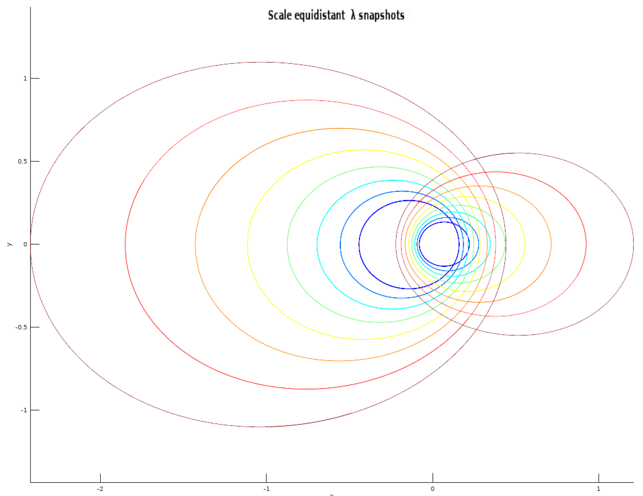
Figure 2.
Streamlines for (62). Blue line corresponds to , above it to ( diverges as for large ), below it to ( vanishes at finite and if integrated through the singularity diverges as ). Note that the blue line is also a small- attractor, meaning that integrating (62) in the negative direction starting from any , gets you arbitrarily close to a physical solution at small enough .
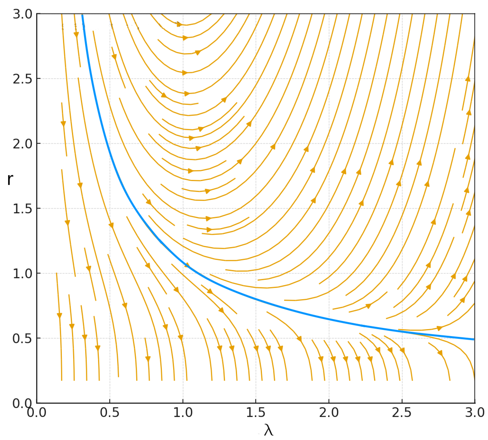
Figure 3.
The rotation curve obtained from (63) by setting (blue). The Newtonian curve for the same parameters (red).
Figure 3.
The rotation curve obtained from (63) by setting (blue). The Newtonian curve for the same parameters (red).
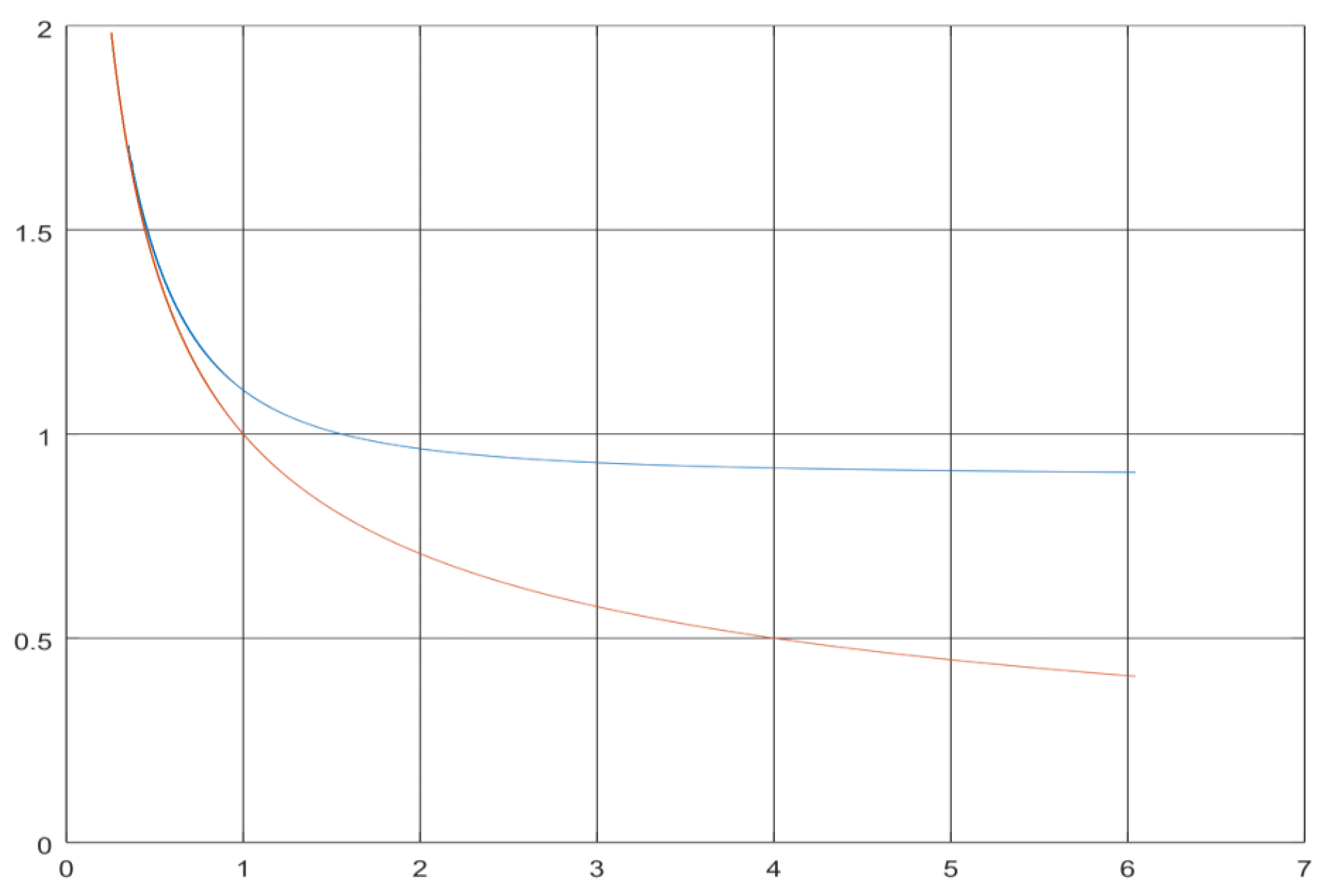
Figure 4.
Retarded world-cylinder of radius r, C, bounded by a time-like three-tube,
, and space-like three-surfaces . This construction produces a smooth T only for .
Figure 4.
Retarded world-cylinder of radius r, C, bounded by a time-like three-tube,
, and space-like three-surfaces . This construction produces a smooth T only for .
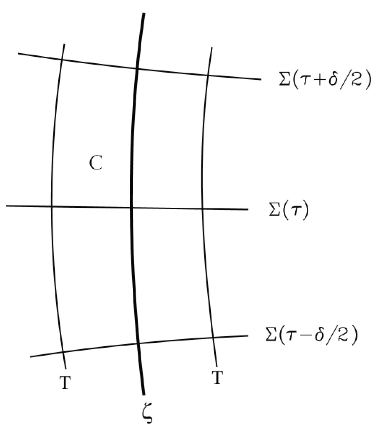
Disclaimer/Publisher’s Note: The statements, opinions and data contained in all publications are solely those of the individual author(s) and contributor(s) and not of MDPI and/or the editor(s). MDPI and/or the editor(s) disclaim responsibility for any injury to people or property resulting from any ideas, methods, instructions or products referred to in the content. |
© 2026 by the authors. Licensee MDPI, Basel, Switzerland. This article is an open access article distributed under the terms and conditions of the Creative Commons Attribution (CC BY) license (http://creativecommons.org/licenses/by/4.0/).
Copyright: This open access article is published under a Creative Commons CC BY 4.0 license, which permit the free download, distribution, and reuse, provided that the author and preprint are cited in any reuse.


