
Submitted:
17 June 2025
Posted:
18 June 2025
You are already at the latest version
Abstract
The warmer air resulting from climate change reduces the lift force on a departing aircraft, potentially reducing its climb angle and causing more engine noise near the airport. Here we study this phenomenon at a selection of 30 European airports. We first formulate and verify a low-complexity model of noise propagation around airports. The model includes anisotropic noise propagation, atmospheric absorption, and multi-engine capability. We use the Airbus A320, but the method could straightforwardly be generalised to other aircraft. We refer to the model as an emulator since it mimics the more comprehensive model against which it is verified. The model is used to calculate the area enclosed by the 50 dB contour (A50), which agrees well with the same metric (using the day-evening-night sound level, Lden) from the parent model (A). Using temperature and pressure data from IPCC simulations of future climate, and using a straightforward relation between climb angle and air density, we assess how climate change could affect climb angles by mid-century (2035–2064). An optimised value of A50 is obtained by efficiently covarying (1) the engine noise at 10 m from the engines and (2) the climb angle under `historical’ conditions (1985–2014). The covariation uses Latin hypercube sampling and the optimum value of A50 differs from A by just 0.05 km2. Median values (across 10 climate models) of climb angle reduction in the future warmer climate are around 1–2%, but individual days can show values as high as 7.5%, which corresponds to an increase in A50 of 0.25 km2. When taking the local population density into account, the number of affected residents per airport increases by over 1,000 in the most densely-populated areas. We conclude that climate change could increase aircraft noise near airports in the coming decades, subjecting thousands of additional people across Europe to engine noise from departing aircraft.
Keywords:
climate change
; noise pollution
; Europe
; scenario
1. Introduction
In this work we examine the effect of climate change on the area enclosed by the 50 dB contour around an ensemble of 30 European airports by considering ‘historical’ (1985-2014) and future projection (2035-2064) timescales. Previous work examined how take-off distance and maximum take-off weight are projected to change in the future [1] and this work uses the same sites as the basis for studying how climb angles may change and how neighbouring populations could be affected.
The Williams et al. [1] study in fact is one of a growing number of studies regarding the perturbation of take-off performance as the world warms (see references therein). However, literature on the effect of climate change on noise around airports is only recently starting to appear. Padhra et al. [2] found – in a 2022, world-first study – that the area of the 60 dB contour around Chios airport has increased by almost 5% in the 25 year period up to 2022. This is attributed to worsened take-off performance due to temperature and headwind perturbations, reducing climb angles. Climate change can also influence atmospheric boundary layer stability [3], which in turn can affect sound propagation [4].
Commerical airports are a major source of noise pollution. For example in 2023, EASA – the European Union Aviation Safety Agency – estimates that almost 3.5 million people in Europe experienced ‘highly annoying’ aircraft-related sound exposure [5]. EASA defines this as an level of at least 55dB which is a weighted average of exposure at different times of the day (i.e. night flights are more disruptive).
Disruption is not limited to the immediately-noticeable auditory impacts on humans. Indeed increased airport noise has been identified as a contributor to cardiovascular disease [6] and increased blood pressure [7] in local populations. Wildlife can also experience negative impacts through induced environmental changes affecting birds, whales and insects amongst others (see e.g. Alquezar and Macedo [8] and Dominoni et al. [9]).
To first order, for a given point in the vicinity of an aircraft up to take-off, the noise exposure is a function of distance from the source and the sound intensity, (usually) measured logarithmically in decibels, dB. However, in reality, there are many other factors which affect the overall level of sound transmission such as thrust level, climb angle and direction and local population density.
Methods of reducing the exposure to noise pollution include Noise Abatement Departure Procedures (NADPs) published by the International Civil Aviation organisation, ICAO [10]. For example, procedures exist for reducing exposure close to and farther away from the airport by changing thrust levels, acceleration profiles and climb angles appropriately [11].
For the remainder of this study however, the thrust level and the historical climb angle are assumed constant, whilst the future climb angles change with air density. Work to understand the effects of climate change on more complex take-off procedures, as well as the economic impacts of climate change on take-off fuel usage is ongoing.
Previously documented tools to produce quantitative studies of airport noise – i.e. involving explicit calculation of noise propagation and resulting contours – include those from:
The present study differs from these tools in that its purpose is to emulate the results found from other models of increased technical and/or scientific complexity. In this context ‘complexity’ can refer to inclusion of different aircraft types such as helicopters [13], aircraft bank angle [14] and considerations of fuel burn and greenhouse gas emissions [14,15]. To achieve this we explore physically reasonable ranges of climb angle and thrust level values.
Emulation techniques are widely used in modelling studies of climate-relevant parameters and tools. For example the FAMOUS climate model [16] simulates (synonymous with ‘emulates’ in this context) the 3D climate response of the higher-resolution HadCM3 model [17] meaning it can produce results faster. In essence it largely uses another model as its ‘ground truth’ target.
Another example of emulation is the statistical techniques which use large ensembles of climate model results to explore parts of parameter space which are not explicitly resolved in the individual model results themselves. An in-depth treatment of this is outside the scope of this article and the interested reader is referred to the review article of Castruccio et al. [18] for further information.
We use the 50dB contour area from IMPACT as our emulation target and use a 10-member Latin hypercube sampling technique to minimise the difference in the values obtained from the two models. We also ensure that the salient features of previously published noise contours are reproduced, although non-trivial differences remain due to the different levels of model complexity.
After establishment of optimised model parameters for present-day conditions we proceed to apply them to future conditions at 30 European airports using a simple relation connecting climb angle and air density. In these future conditions – see Williams et al. [1] for details – air density shows an overall decrease, largely due to increased temperatures. This then leads to smaller climb angles and an increased noise pollution footprint.
2. Materials and Methods
The coordinate system used for noise intensity calculations at ground level is two dimensional () centred on the aircraft’s take-off location and extends a set number of multiples of the runway length, , in and . To simplify the calculations, the runway is assumed to run perfectly north-south (the y direction) and the true runway orientation is applied later by rotating the entire grid using third order spline interpolation [19]
To account for the vertical, z, coordinate, after take-off the aircraft is assumed to climb with constant angle, . The Euclidean distance from the aircraft to each point in the grid is then calculated for every in the trajectory. The resulting noise level presented below in Figure 4 is then simply the maximum value at each in the aircraft’s path.
Assuming sound radiation is isotropic, its intensity, I, is assumed to reduce with distance from the sources – engines – as an inverse square law,
where is the sound (power) intensity at a reference distance, , from the source.
In general, the exponent of r may differ from 2, especially very close to the source, but we do not consider this further here.
The power intensity at some arbitrary distance from the aircraft, I, has units of but usually it is the intensity of the sound in decibels, which we want to know, where (using throughout)
Combining the relations for I and gives
Sound intensity (in dB) can also be reduced due to absorption processes – assumed proportional to distance from the source – and this is included using a constant coefficient of absorption, , multiplied by a factor proportional to the ratio of the air density to the sea-level ISA value, . In general this relationship can be more complex [20] but we do not consider this further here.
We use a constant value of dB · m−1, which is a good approximation for, say, 1 kHz and 50% relative humidity [21].
This gives our final equation for sound fall-off with distance,
with kg·m−3.
The discussion above assumes that an aircraft engine emits as a point source of size 10 m. For explicit consideration of multiple engines (two here), the following expression is used,
where each of are described by equation 4.
Figure 1 shows the dB contours around two point sources at varying distances, d. In practice, for the size of the domain considered here – Figure 1(a) – the engines are close enough to be considered as a point source of intensity described by equation 5 with . In general however, for widely spaced sources – Figure 1(b, c) – the power distribution is not radially symmetric close to the sources. For the purposes of this work, it is the ‘far field‘ () behaviour which is of primary interest.
In practice, the sound emission from a standard turbofan engine is anisotropic and highly complex – e.g. [22,23] – and is parameterised here by increasing the sound levels both behind and in front of the engine’s intake axis (the y direction, i.e. before taking the runway bearing into account) compared to the lateral direction. This is shown diagrammatically in Figure 2 and described mathematically by
where is the angle over which multiple take-off paths are run in order to represent the enhanced power intensity in the direction parallel to the direction of travel and is an empirically determined scaling parameter. Each path is rotated around the centre of the grid which is defined as the end of the runway, i.e. the starting position of travel (for the , central estimate) is , .
3. Effect of Climate Change on Climb Angle
Recent work has quantified how take-off performance – distance required, maximum payload – may change in the future for a selection of Europe’s busiest airports [1]. As greenhouse gases accumulate in the atmosphere and the air warms, the air density tends to decrease in line with the ideal gas law,
where P is the air pressure, is the air density, is the specific gas constant for air (287.05 J · kg−1 · K−1) and T is the temperature.
Using 10 state of the art climate models forced with three different scenarios of 2035-2064 greenhouse gas forcing compared to 1985-2014, daily time series of temperature and air pressure were obtained and from these values the predicted air pressure was calculated. The future scenarios used (Shared Socioeconomic Pathways, SSPs) are SSP1-2.6, SSP3-7.0 and SSP5-8.5. The format SSP- refers to the SSP ‘family’, and the net radiative forcing per m2 at 2100, . These can be considered as low, medium and high magnitude climate change amounts respectively [24].
The dependence of aircraft climb angle is a highly complex function of many variables such as atmospheric conditions, thrust level, aircraft variant and altitude (see [25] and references therein). However, in order to provide a straightforward and accessible presentation of this in software, we assume the following force balance at take-off,
where T, D and W are the thrust, drag and weight respectively and is the climb angle (see e.g. [26], supplementary material part 2).
We further make the assumption that both T and D are proportional to air density, which is a good approximation assuming incompressible flow in International Standard Atmosphere conditions [27]. Combining the above assumptions, for historical (‘1’) and climate change affected conditions (‘2’) respectively we have
or equivalently, since are proportional to density, ,
and
Therefore we now have an equation for describing how the climate change-affected climb angle, can be calculated as a function of the historical and future air densities. The historical climb angle, is assumed constant in this work and its range of validity is discussed in Section 4.
4. Parameter Uncertainty and Latin Hypercube Parameter Sampling
In the model described above – indeed as is the case for any model – there are approximations and parameterisations. For example, the sound intensity near the source and the initial climb angle are both assumed constant, neither of which is strictly adhered to in real flight operations. Additionally, the inverse square relation and constant absorption coefficient described in Equation 4 deviate from these idealised mathematical formulations due to, e.g., ground reflection and sound frequency dependence respectively [23,28].
To account for these uncertainties, we have established plausible ranges of and and then used Latin hypercube sampling (LHS) to establish optimum parameter values. LHS efficiently samples the parameter space defined by the input variables () to avoid having to exhaustively sample the full 2-dimensional landscape of possible combinations [29].
We used the area enclosed by the 50dB noise contour around San Sebastian airport from the IMPACT1 model – – as our verification target. The 50dB level is a commonly used baseline for aircraft-related noise disturbance [30,31] and is broadly equivalent to that of a residential, suburban environment [32].
This site is of particular interest since it straddles both a national border (France, Spain) and a coastline as well as having a short runway.
The output for the model presented here represents one take-off procedure, and this is compared against the day-evening-night level, output from IMPACT. This represents average noise exposure over a 24 hour period [33] and is given by
which shows the 5 and 10dB ‘penalties’ which are applied to evening and night flights respectively. Using alleviates some of the inherent issues in the comparison with IMPACT’s greater complexity and capability.
To obtain initial estimates of bounds for and we first calculated the area enclosed by the 50 dB contour () using , which is given as a typical value in Gratton et al. [26] and dB for each engine.
The choice of 100 dB is the value at 10 m from an engine with source intensity of 120 dB assuming isotropic transmission from 1 m away (e.g. Huang and Zheng [34]). This 10 m ‘buffer’, as well as being of the order of the inter-engine distance, , also allows for some alleviation of the reflection effects referred to above.
Estimates and measurements of jet engine sound intensity vary significantly depending on the type and age of the engine, the atmospheric conditions and the precise noise metric used [35]. Therefore – and since our model is intended as an emulator rather than a simulator – the precise values used are not crucial as long as they emulate the equivalent value from IMPACT.
Using dB and , we obtain km2, compared to km2, an overestimate of ≈13%. Considering the assumptions and simplifications in the present model this is an encouragingly small discrepancy. However it is important to perturb the parameter assumptions to make sure that this is not entirely serendipitous.
The flight operation used in the calculation in IMPACT, when averaged over its first 10,000 ft, is approximately . For , from its maximum at ‘take-off roll’, the power setting is reduced by up to over the course of the first few nautical miles of its trajectory. A 40% decrease is equivalent to roughly 2 dB and so we use dB and . The results of this sampling are shown in Figure 3 for a sample size, N, of 10.
Figure 3 shows that the 6th member of the LHS distribution gives the best agreement between and ; a difference of 0.05 km2. This corresponds to dB and and these values are used for the remainder of this study.
5. Results
Figure 4 shows the results of the verification procedure described above using San Sebastian airport for the parameters shown in Table 1.

Table 1.
Parameters used for the generation of the Figure 4. The mx2t24 and values are means of 30 years of historical data from the ACCESS-ESM1-5 climate model and are only used in the absorption calculation.
Table 1.
Parameters used for the generation of the Figure 4. The mx2t24 and values are means of 30 years of historical data from the ACCESS-ESM1-5 climate model and are only used in the absorption calculation.
| Parameter | Value | unit |
|---|---|---|
| 99.01 | dB | |
| 20 | – | |
| 32 | – | |
| 7.28 | – | |
| 4.77 | km2 | |
| 4.82 | km2 | |
| mx2t24 | 20.6 | K |
| 1019.2 | hPa | |
| [36] | 11.2 | m |
| [1] | 1800 | m |
Figure 4.
The extent of the 50, 55, and 60 dB contours around San Sebastian airport calculated using the present emulator framework. The take-off direction is from south west to north east.
Figure 4.
The extent of the 50, 55, and 60 dB contours around San Sebastian airport calculated using the present emulator framework. The take-off direction is from south west to north east.

Figure 4 shows the 50, 55, and 60 dB noise contours around San Sebastian airport. The effect of the anisotropic power intensity, amplified in the direction of travel (to the north east in this case) and the tapering off of the sound intensity as the aircraft climbs.
The overall shape of the contours is in good empirical agreement with previous work by, e.g., Tlałka and Rzucidło [37], Sahai et al. [38] and in policy documentation from the US Federal Aviation Administration [39]. Indeed, considering the relative simplicity of our model, the agreement with previous results is encouraging. In any case, the precise shape does not change any of the conclusions drawn below since our we are examining changes to noise contour area (and affected populations) rather than absolute values.
5.1. Effect of Atmospheric Conditions on Climb Angle
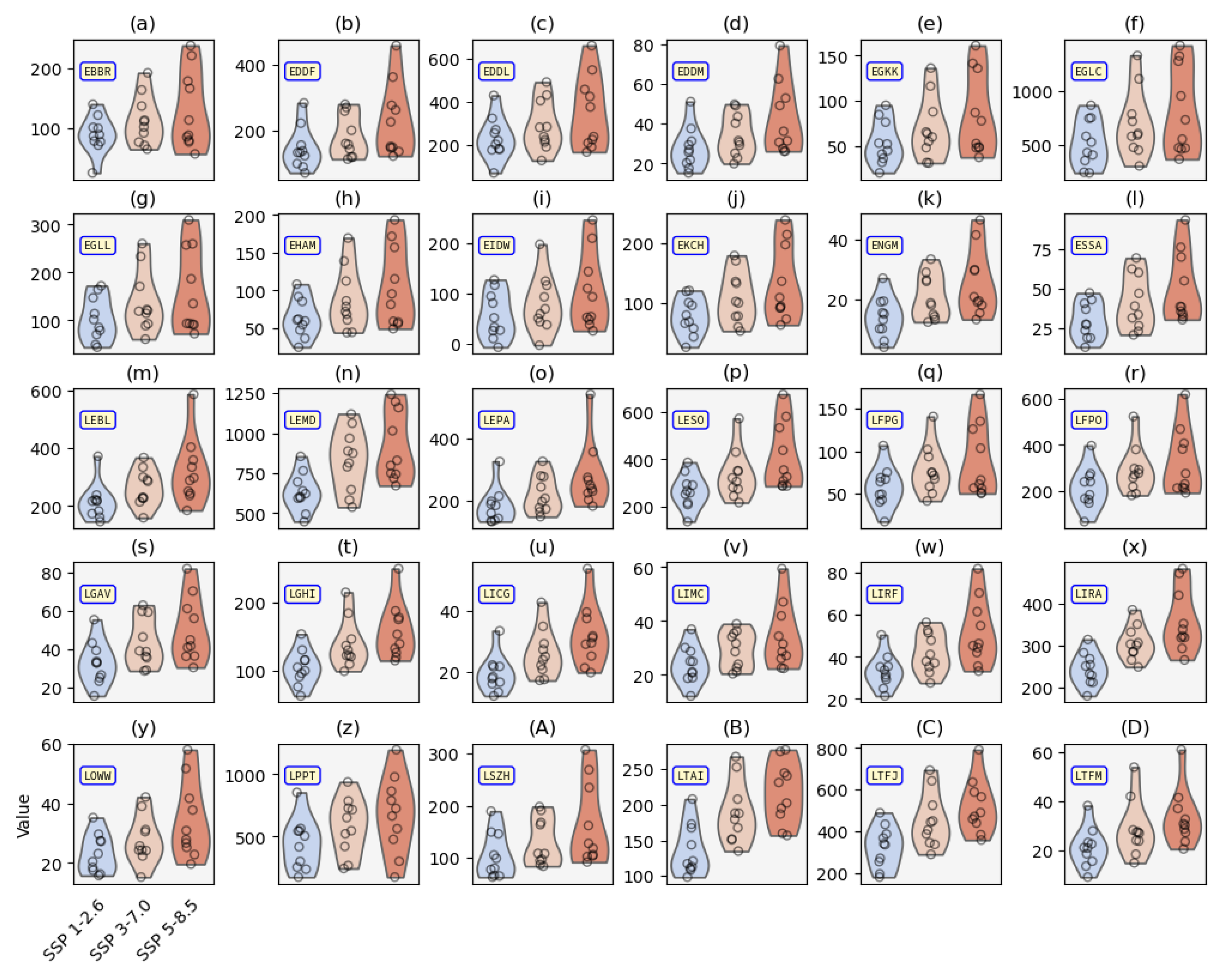
Figure 5 shows the projected increase in around each site as a function of the climate change scenario used in the future modelling. The format of this figure uses ‘violin’ plots which show each individual model’s mean value (symbols) and with a width which shows their distribution.
Broadly speaking, the effect on shown in Figure 5 is independent of the airport, although there is significant inter-model spread within the individual scenarios’ results. The most extreme scenario considered, SSP5-8.5, shows the largest variability. This is the expected behaviour – as previously noted in Williams et al. [1] – because of the range of climate sensitivity responses from the models in the ensemble; that is, the sensitivity of temperature change to changing greenhouse gas concentrations.
The individual values shown in Figure 5 (circles) show the response of for each climate model to the mean change in air density in each of the scenarios compared to the historical period. This averaging masks the day-to-day variability in the summer temperatures and pressures. To investigate the full distribution of these values, Figure 6 shows (daily maximum) temperature, daily mean pressure and resulting values for UKESM1-0-LL and SSP5-8.5 at San Sebastian.
Figure 6 shows the individual values for each day in the period 2035-2064 for SSP5-8.5 and clearly shows the expected decrease in with increasing temperature as discussed above. It also shows decreases as high as 7.5% (blue values). This corresponds to – cf. Table 1 – or equivalently km2 – from Equation 13. This is over 5% of , albeit with a relatively low occurrence frequency.
In the next section we examine how these geometric variables can be translated into quantified impacts on local populations.
5.2. Climate Change Impacts on Residential Populations Near Airports
Although the changes to shown in Figure 5 may appear insignificant at first, we shall see below that once the population density around airports is taken into account (which for some airports exceeds ), the number of additional people, compared to historical climate conditions, potentially affected by these changes can be significant, even without considering extreme values (Figure 6).
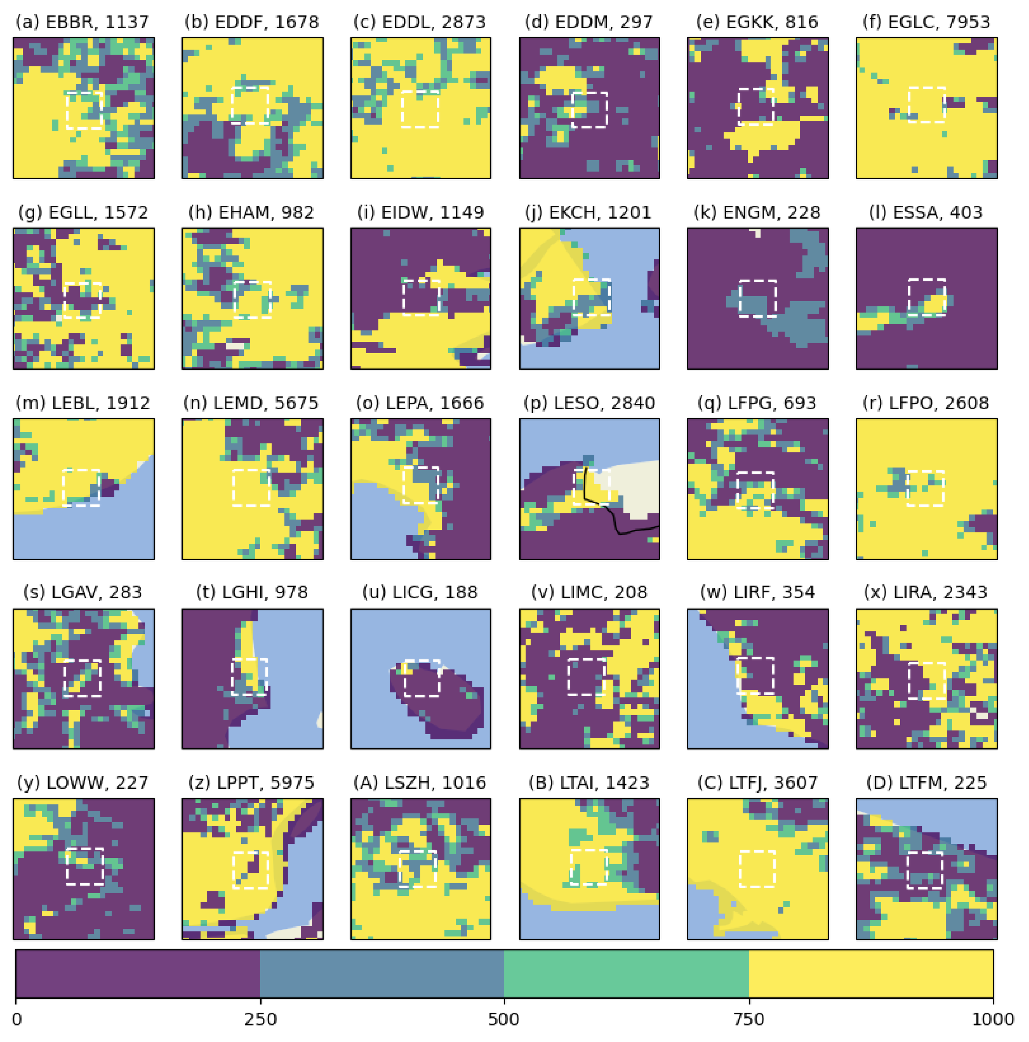
With this in mind we use the WorldPop dataset at 30 arc second (≈1km) resolution which has been adjusted to coincide with UN data by the data curators (i.e. not part of this work) [40]. Figure 7 shows population densities around our 30 study sites. Going forward, to estimate the number of people affected by noise in the vicinity of these airports, we use the average population density in a ±3 km box (white dashed lines in Figure 7) to ensure realistic values are used. Without this additional ‘smoothing’ step, some sites give spuriously low (or even vanishing, in the case of Milan Airport) density values which may lead to underestimation of the number of people affected.
Ultimately, the metric of primary interest in this study is the number of people affected by changes to the area enclosed by a given dB contour.
Figure 8 shows the increase in the number of people affected by noise pollution for each climate change scenario, calculated by multiplying the population density (Figure 7) by the fractional increase in the area of the 50dB contour (Figure 5) and multiplying its model ensemble mean area in the historical simulations.
The variation in the values in Figure 8 is striking, with values ranging from a few tens to several thousand additional residents within the 50 dB contour. This is primarily a reflection of the population density values shown in Figure 7, however there are some other noteworthy aspects of this final set of results. Firstly, the model ensemble-spread is large. This in itself is not surprisingly, indeed it is expected due to the large underlying ensemble spread in recent model intercomparisons compared to earlier ones, e.g. Meehl et al. [41]. It is possible that using a larger number of models in future studies may allow the error bars in Figure 8 to be reduced.
The resolution of the raw input data itself (∼100 km) is also an aspect which will lead unavoidably to increased similarity between the results obtained from closely neighbouring sites. For example, although the model data used in this study has undergone data processing and bias correction, the three airports studied in the London region for example are close enough for their overall climate response to be essentially the same. This of course has the distinct advantage of making the datasets small enough to be easily distributable and processable on standard PCs and data connections, however it would be of great interest to consider higher resolution (raw) input datasets, especially with the advent of new, ultra-high resolution regional climate projections [42].
6. Conclusions
In this work we have presented the results of a model which projects the climate change-induced changes to populations affected by noise pollution at 30 European airports.
The model was optimised using Latin hypercube sampling of two key parameters – near-engine sound intensity and climb angle – to emulate the area enclosed by the 50dB day-evening-night averaged sound level () contour surrounding San Sebastian airport produced by the more complex IMPACT model.
After this verification step, we use results from 10 state-of-the-art climate models to project how climb angle may change by mid-century compared to a historical baseline. This is based on three possible future scenarios of greenhouse gas emissions which cause varying degrees of perturbation to air temperature, and ultimately to air density, which is the input parameter in the climb angle calculation method used.
By combining the projections of the changes to and contemporary local population density, changes to the number of noise-impacted residents has been estimated. This has been done for all 30 airports and each climate change scenario with the differing warming responses of the climate models providing a robust uncertainty estimate.
Although the fractional values are broadly uniform, ranging from approximately 1-2%, the population density changes vary from ≈ 200-8000 km−2 which similarly affects the change to the absolute number of residents affected.
This response of the model-ensemble values is consistent across the site ensemble, yet these values are averaged across the respective 30-year periods. By considering the day-to-day distributions of temperature and pressure yields insights into how extreme values may change and in the most extreme climate-change scenario considered, values of as high as 7.5% could result. This corresponds to a change of approximately 0.25km2 in the area enclosed by the 50 dB contour, or potentially more than one thousand affected residents in the more populated areas.
There are several key aspects which should be borne in mind in future use of the model; either as presented here, or in future model development.
Firstly, the present model assumes simple force balance leading to a linear, analytical relation between air density and climb angle. In practice this will be complicated by factors such as variations in thrust level, headwind and aircraft type, for example. Because of these uncertainties, and the flexibility and relative simplicity of the model, future studies using different functional relationships are encouraged.
A related ‘upgrade’ to the current model could include more detailed verification metrics. The present study uses the area enclosed by the 50 dB noise contour, and compares this to an equivalent () value from the IMPACT model. Future work could include using a range of decibel values and/or a larger number of evaluation target models.
From a geographical perspective, this study – by design – is limited to European airports, and so a further extension to this work should include a larger, ideally global, domain. To enable this, the site specificity and raw climate model data bias correction steps – see Williams et al. [1] and references therein – could be embedded within a common software framework. This would have the distinct advantage of being able to the address the intimately related issues of noise pollution and take-off performance restrictions in a unified manner.
Author Contributions
Conceptualization, J.W., P.D.W., M.V., A.P., G.G. and S.R.; methodology, J.W., P.D.W., A.P., G.G. and S.R.; software, J.W., and M.V.; validation, J.W., M.V. and P.D.W.; formal analysis, J.W., P.D.W., and M.V.; investigation, J.W., P.D.W. and M.V.; resources, J.W., P.D.W., M.V.; data curation, J.W. and M.V.; writing, J.W. and P.D.W.; visualization, J.W. supervision, P.D.W.; project administration, P.D.W.; funding acquisition, P.D.W. All authors have read and agreed to the published version of the manuscript.
Funding
The work of J.W., P.D.W. and M.V. for this article is part of the AEROPLANE project, which is supported by the SESAR 3 Joint Undertaking and its founding members, Grant Agreement ID 101114682, https://cordis.europa.eu/project/id/101114682, accessed on 10 June 2025. S.R. was funded by the Environmental and Networking Technologies and Applications Unit (ENTA) of the Athena Research Center.
Data Availability Statement
The raw data presented in the study are openly available in the Earth System grid Federation—ESGF—repository [43]
Acknowledgments
We thank the World Climate Research Programme (WCRP), which, through its Working Group on Coupled Modelling, coordinated and promoted CMIP6. We acknowledge the climate modelling groups for generating and making available their model output, the Earth System Grid Federation (ESGF) for archiving the data and providing access, and the many funding agencies who support the vital work of CMIP and the ESGF. We also acknowledge the computational services provided by the University of Reading’s Academic Computing Cluster (RACC) and associated research software engineering staff. Licencing and technical support for the IMPACT model was provided by EUROCONTROL.
Conflicts of Interest
The authors declare no conflicts of interest.
Abbreviations
The following abbreviations are used in this manuscript:
| AEDT | Aviation Environmental Design Tool |
| ANCON | Aircraft Noise Contour (model) |
| CMIP6 | 6th Coupled Model Intercomparison Project |
| EASA | European Union Aviation Safety Agency |
| FAMOUS | Fast Met Office/UK Universities Simulator |
| HadCM3 | Hadley Centre Coupled Model version 3 |
| ICAO | International Civil Aviation Organisation |
| IMPACT | Integrated 68 Aircraft Noise and Emissions Modelling Platform |
| INM | Integrated Noise Model |
| ISA | International Standard Atmosphere |
| LHS | Latin hypercube Sampling |
| SSP | Shared Socioeconomic Pathway |
Appendix A
Table A1.
Mathematical symbols used.
| Symbol | Definition |
|---|---|
| I | Sound intensity |
| r | Distance from sound source |
| Air density | |
| Air density under International Standard Atmosphere conditions at sea level | |
| Coefficient of sound absorption | |
| Angle over which noise anisotropy is calculated | |
| Empirical scaling parameter controlling the shape of the noise anisotropy | |
| Specific gas constant for air | |
| Climb angle | |
| T | Thrust |
| D | Drag |
| W | Weight |
| Day-evening-night noise level | |
| Area enclosed by the 50 dB contour in the emulator. | |
| Area enclosed by the 50 dB contour in the IMPACT model. |
References
- Williams, J.; Williams, P.D.; Guerrini, F.; Venturini, M. Quantifying the Effects of Climate Change on Aircraft Take-Off Performance at European Airports. Aerospace 2025, 12, 165. [CrossRef]
- Padhra, A.; Rapsomanikis, S.; Gratton, G.; Williams, P.D. The Impacts of Climate Change on Aircraft Noise Near Airports. In Proceedings of the Proceedings of the 4th International Aviation Management Conference (IAMC 2022), Dubai, UAE, November 21-22 2022.
- Caserini, S.; Giani, P.; Cacciamani, C.; Ozgen, S.; Lonati, G. Influence of climate change on the frequency of daytime temperature inversions and stagnation events in the Po Valley: historical trend and future projections. Atmospheric Research 2017, 184, 15–23. [CrossRef]
- Hole, L.R.; Hauge, G. Simulation of a morning air temperature inversion break-up in complex terrain and the influence on sound propagation on a local scale. Applied Acoustics 2003, 64, 401–414. [CrossRef]
- European Union Aviation Safety Agency (EASA). European Aviation Environmental Report 2025, 2025. Accessed: 2025-05-19.
- Stansfeld, S. Airport noise and cardiovascular disease. British Medical Journal 2013, 347. [CrossRef]
- Black, D.A.; Black, J.A.; Issarayangyun, T.; Samuels, S.E. Aircraft noise exposure and resident’s stress and hypertension: A public health perspective for airport environmental management. Journal of Air Transport Management 2007, 13, 264–276. The Air Transport Research Society’s 10th year Anniversary, Nagoya Conference, 2006, . [CrossRef]
- Alquezar, R.D.; Macedo, R.H. Airport noise and wildlife conservation: What are we missing? Perspectives in Ecology and Conservation 2019, 17, 163–171. [CrossRef]
- Dominoni, D.M.; Greif, S.; Nemeth, E.; Brumm, H. Airport noise predicts song timing of European birds. Ecology and Evolution 2016, 6, 6151–6159. [CrossRef]
- International Civil Aviation Organization. Review of Noise Abatement Procedure Research & Development and Implementation Results, 2007. Accessed: 2025-02-10.
- Bhanpato, J.; Puranik, T.G.; Mavris, D.N. Data-Driven Analysis of Departure Procedures for Aviation Noise Mitigation. Engineering Proceedings 2021, 13. [CrossRef]
- Ollerhead, J. The CAA aircraft noise contour model: ANCON version 1; Uk Civil Aviation Authority, 1992.
- Boeker, E.R.; Dinges, E.; He, B.; Fleming, G.; Roof, C.J.; Gerbi, P.J.; Rapoza, A.S.; Hermann, J. Integrated Noise Model (INM) Version 7.0 Technical Manual. Technical Report FAA-AEE-08-01, John A. Volpe National Transportation Systems Center (U.S.), Acoustics Facility; ATAC Corporation, 2008.
- Aviation Environmental Design Tool (AEDT) Version 3g Technical Manual. Technical report, Federal Aviation Administration, Office of Environment and Energy, 2024. Technical manual for AEDT Version 3g. Developed by the U.S. DOT Volpe National Transportation Systems Center.
- EUROCONTROL. Integrated Aircraft Noise and Emissions Modelling Platform (IMPACT), 2025. Accessed: 2025-05-20.
- Jones, C.; Gregory, J.; Thorpe, R.; Cox, P.; Murphy, J.; Sexton, D.; Valdes, P. Systematic optimisation and climate simulation of FAMOUS, a fast version of HadCM3. Climate Dynamics 2005, 25, 189–204. [CrossRef]
- Gordon, C.; Cooper, C.; Senior, C.A.; Banks, H.; Gregory, J.M.; Johns, T.C.; Mitchell, J.F.; Wood, R.A. The simulation of SST, sea ice extents and ocean heat transports in a version of the Hadley Centre coupled model without flux adjustments. Climate dynamics 2000, 16, 147–168.
- Castruccio, S.; McInerney, D.J.; Stein, M.L.; Crouch, F.L.; Jacob, R.L.; Moyer, E.J. Statistical Emulation of Climate Model Projections Based on Precomputed GCM Runs. Journal of Climate 2014, 27, 1829 – 1844. [CrossRef]
- Community, S. SciPy: Scientific Library for Python, 2023. Accessed: 2025-02-06.
- Beranek, L.L.; Mellow, T. Acoustics: Sound Fields and Transducers; Academic Press: San Diego, CA, 2012.
- Smith, J.O. Physical Audio Signal Processing; accessed February 2025. online book, 2010 edition.
- Xue, R.; Jiang, J.; Zheng, X.; Gong, J.l.; Jackson, A. Study of Noise Reduction Based on Optimal Fan Outer Pressure Ratio and Thermodynamic Performance for Turbofan Engines at Conceptual Design Stage. International Journal of Aeronautical and Space Sciences 2019, 21, 439–450.
- Zaporozhets, O.; Tokarev, V.; Attenborough, K. Aircraft noise characteristics on the ground and in the atmosphere. Journal of Sound and Vibration 2014, 333, 1043–1064. [CrossRef]
- O’Neill, B.C.; Tebaldi, C.; van Vuuren, D.P.; Eyring, V.; Friedlingstein, P.; Hurtt, G.; Knutti, R.; Kriegler, E.; Lamarque, J.F.; Lowe, J.; et al. The Scenario Model Intercomparison Project (ScenarioMIP) for CMIP6. Geoscientific Model Development 2016, 9, 3461–3482. [CrossRef]
- Takahashi, T.T.; Sóbester, A. Climb Performance Anomalies in ‘Real’ Atmospheric Conditions. AIAA 2023.
- Gratton, G.; Padhra, A.; Rapsomanikis, S.; Williams, P.D. The impacts of climate change on Greek airports. Climatic Change 2020, 160, 219–231. [CrossRef]
- Marchman III, J.F., Aerodynamics and Aircraft Performance; Virginia Tech Publishing, 2019; chapter 4.
- Filippone, A. Aircraft noise prediction. Progress in Aerospace Sciences 2014, 68, 27–63. [CrossRef]
- Gregoire, L.J.; Valdes, P.J.; Payne, A.J.; Kahana, R. Optimal tuning of a GCM using modern and glacial constraints. Climate Dynamics 2011, 37, 705–719. [CrossRef]
- Roca-Barceló, A.; Nardocci, A.; de Aguiar, B.S.; Ribeiro, A.G.; Failla, M.A.; Hansell, A.L.; Cardoso, M.R.; Piel, F.B. Risk of cardiovascular mortality, stroke and coronary heart mortality associated with aircraft noise around Congonhas airport, São Paulo, Brazil: a small-area study. Environmental Health 2021, 20, 59. [CrossRef]
- Baudin, C.; Lefèvre, M.; Champelovier, P.; Lambert, J.; Laumon, B.; Evrard, A.S. Self-rated health status in relation to aircraft noise exposure, noise annoyance or noise sensitivity: the results of a cross-sectional study in France. BMC Public Health 2021, 21, 116. [CrossRef]
- Purdue University Department of Chemistry. Biosafety Levels, n.d. Accessed: 2025-05-16.
- Directive 2002/49/EC of the European Parliament and of the Council of 25 June 2002 relating to the assessment and management of environmental noise. https://eur-lex.europa.eu/legal-content/EN/TXT/PDF/?uri=CELEX:32002L0049, 2002. Official Journal of the European Communities, L 189, 18/07/2002, pp. 12–26.
- Huang, J.; Zheng, L. Noise analysis of the turbojet and turbofan engine tests. Proceedings of the Institution of Mechanical Engineers, Part G 2014, 228, 2414–2423. [CrossRef]
- Gély, D.; Márki, F. Understanding the Basics of Aviation Noise. In Aviation Noise Impact Management; Leylekian, L.; Covrig, A.; Maximova, A., Eds.; Springer, 2022; pp. 1–9. [CrossRef]
- Airbus S.A.S.. A320 Aircraft Characteristics - Airport and Maintenance Planning. Airbus S.A.S., Blagnac Cedex, France, revision no. 44 ed., 2024. Accessed June 10, 2025.
- Tlałka, F.; Rzucidło, P. Modeling and Analysis of Noise Emission Using Data from Flight Simulators. Applied Sciences 2023, 13. [CrossRef]
- Sahai, A.K.; Snellen, M.; Simons, D.G.; Stumpf, E. Aircraft Design Optimization for Lowering Community Noise Exposure Based on Annoyance Metrics. Journal of Aircraft 2017, 54, 3421–3432. [CrossRef]
- Federal Aviation Administration. Basics of Aircraft Noise, n.d. Accessed: 2025-06-11.
- WorldPop.; for International Earth Science Information Network (CIESIN), C. Global High Resolution Population Denominators Project. https://dx.doi.org/10.5258/SOTON/WP00675, 2018. Funded by The Bill and Melinda Gates Foundation (OPP1134076).
- Meehl, G.A.; Senior, C.A.; Eyring, V.; Flato, G.; Lamarque, J.F.; Stouffer, R.J.; Taylor, K.E.; Schlund, M. Context for interpreting equilibrium climate sensitivity and transient climate response from the CMIP6 Earth system models. Science Advances 2020, 6, eaba1981. [CrossRef]
- Ban, N.; Caillaud, C.; Coppola, E.; Pichelli, E.; Sobolowski, S.; Adinolfi, M.; Ahrens, B.; Alias, A.; Anders, I.; Bastin, S.; et al. The first multi-model ensemble of regional climate simulations at kilometer-scale resolution, part I: evaluation of precipitation. Climate Dynamics 2021, 57, 275–302. [CrossRef]
- Eyring, V.; Bony, S.; Meehl, G.A.; Senior, C.A.; Stevens, B.; Stouffer, R.J.; Taylor, K.E. Overview of the Coupled Model Intercomparison Project Phase 6 (CMIP6) experimental design and organization. Geoscientific Model Development 2016, 9, 1937–1958. [CrossRef]
| 1 |
Figure 1.
Illustrative power intensity contours around two points sources (circles) for varying inter-source distance, d. (a) , (b) , (c) ,. The contours in each figure are identical and converge for .
Figure 1.
Illustrative power intensity contours around two points sources (circles) for varying inter-source distance, d. (a) , (b) , (c) ,. The contours in each figure are identical and converge for .
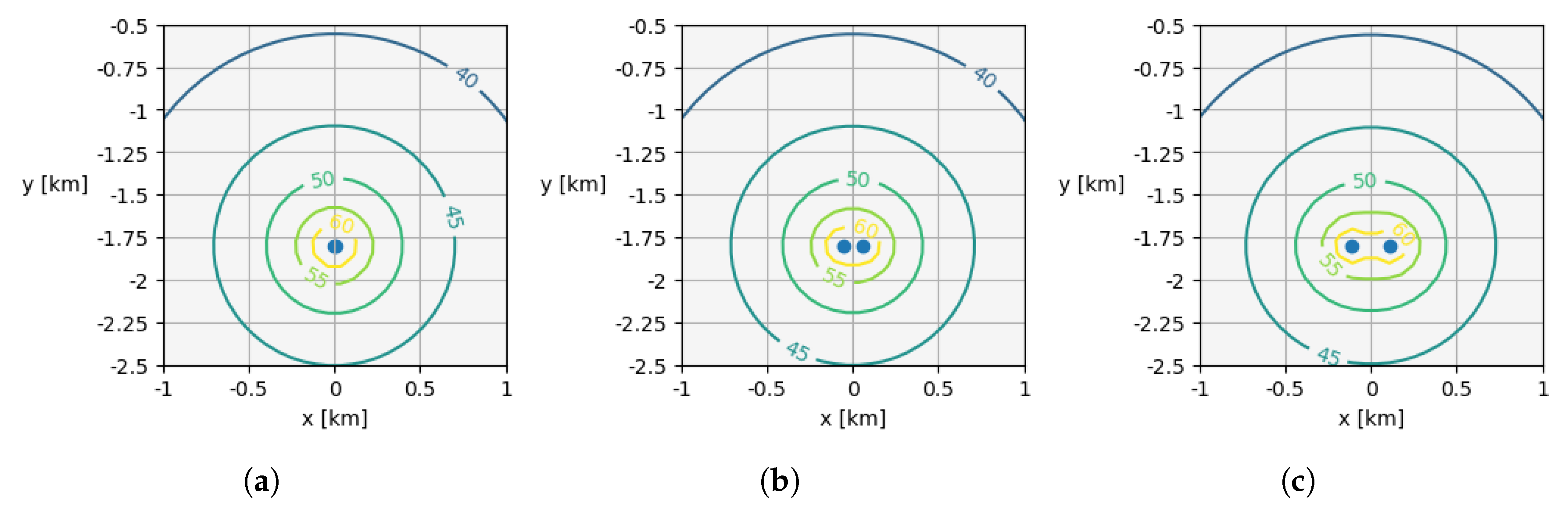
Figure 2.
(a) Spherically isotropic sound propagation and (b) modified to include a preferentially amplified sound intensity in the forward and reverse directions. Also shown in (b) are the angle over which the sound is amplified, as well as their respective weightings.
Figure 2.
(a) Spherically isotropic sound propagation and (b) modified to include a preferentially amplified sound intensity in the forward and reverse directions. Also shown in (b) are the angle over which the sound is amplified, as well as their respective weightings.
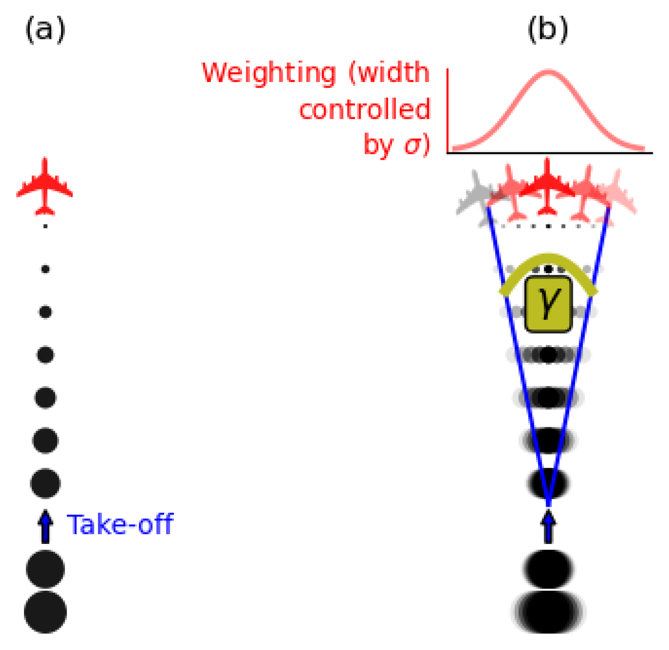
Figure 3.
(a) Scatter plot of the values of and () directly from the Latin Hypercube sampling. The optimum values of and are shown by the values corresponding to the lowest shown value in (b), i.e. where the value of of is closest to ; (b) Values of for each value, i, in the sampling distribution; (c) Illustrative values as a function of using the optimised value shown in (a).
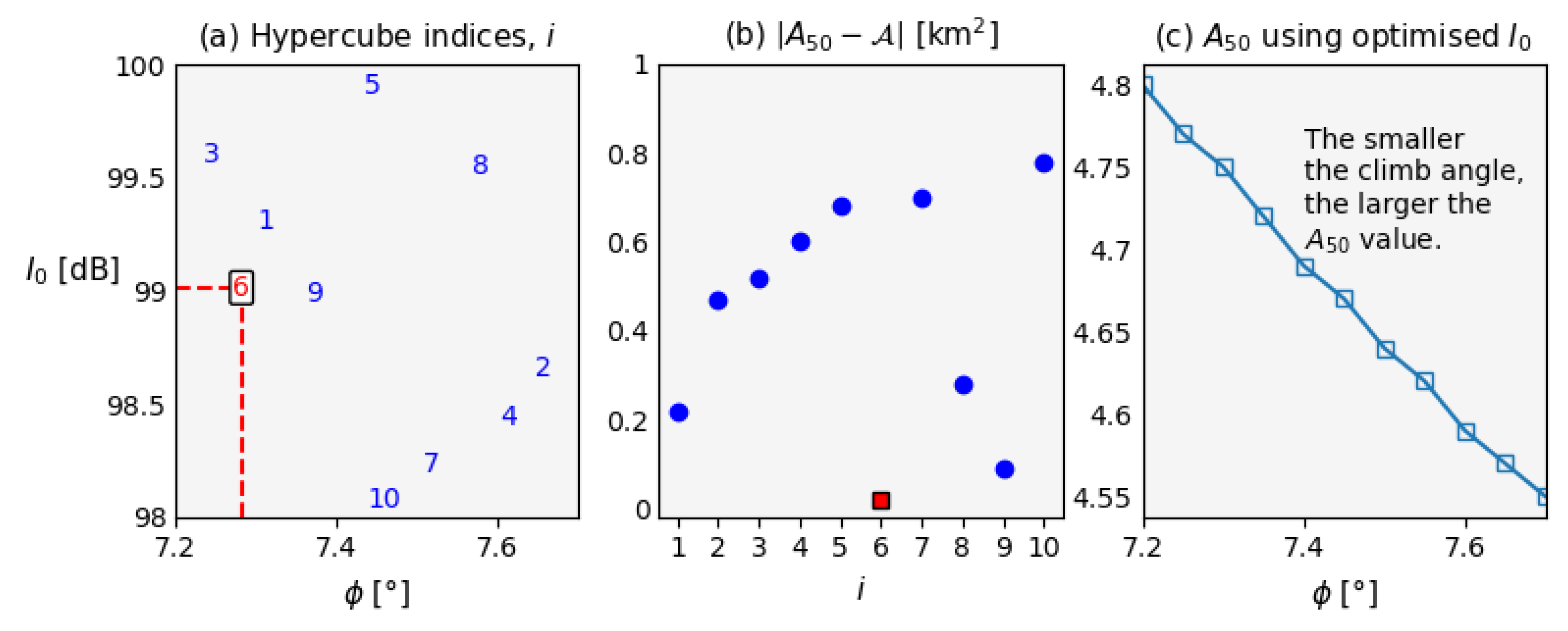
Figure 5.
Percentage change to the area enclosed by the 50 dB contour () for each of the study sites and climate change scenarios studied as a function of climate change scenario.
Figure 5.
Percentage change to the area enclosed by the 50 dB contour () for each of the study sites and climate change scenarios studied as a function of climate change scenario.
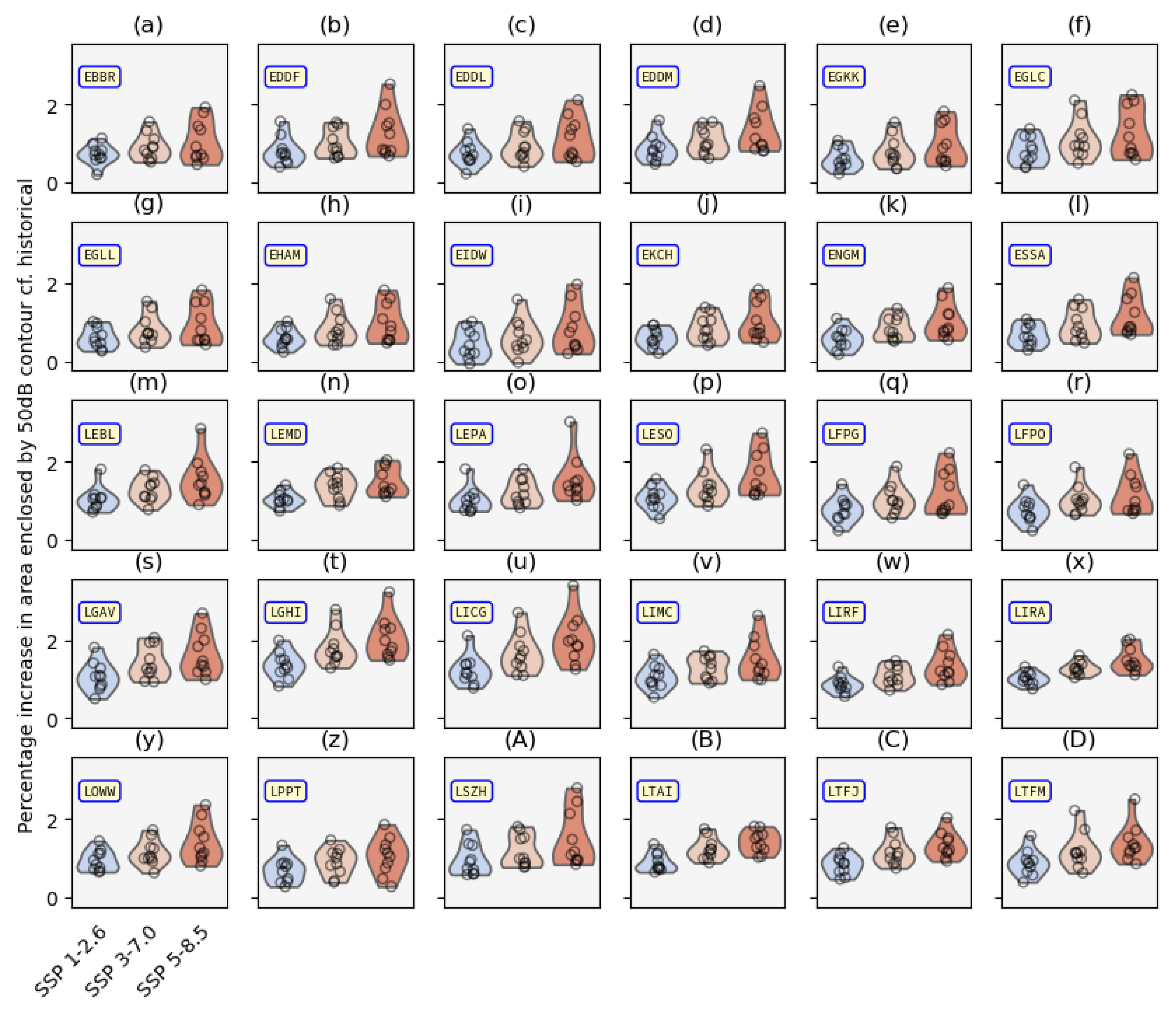
Figure 6.
Scatter plot of calculated climb angles (compared to the assumed historical constant value in Table 1) for San Sebastian airport under SSP5-8.5 conditions using the UKESM1-0-LL climate model [1]. The marginal plots on the top and right show the relative frequency of occurrence of the daily maximum temperature and daily mean pressure values respectively.
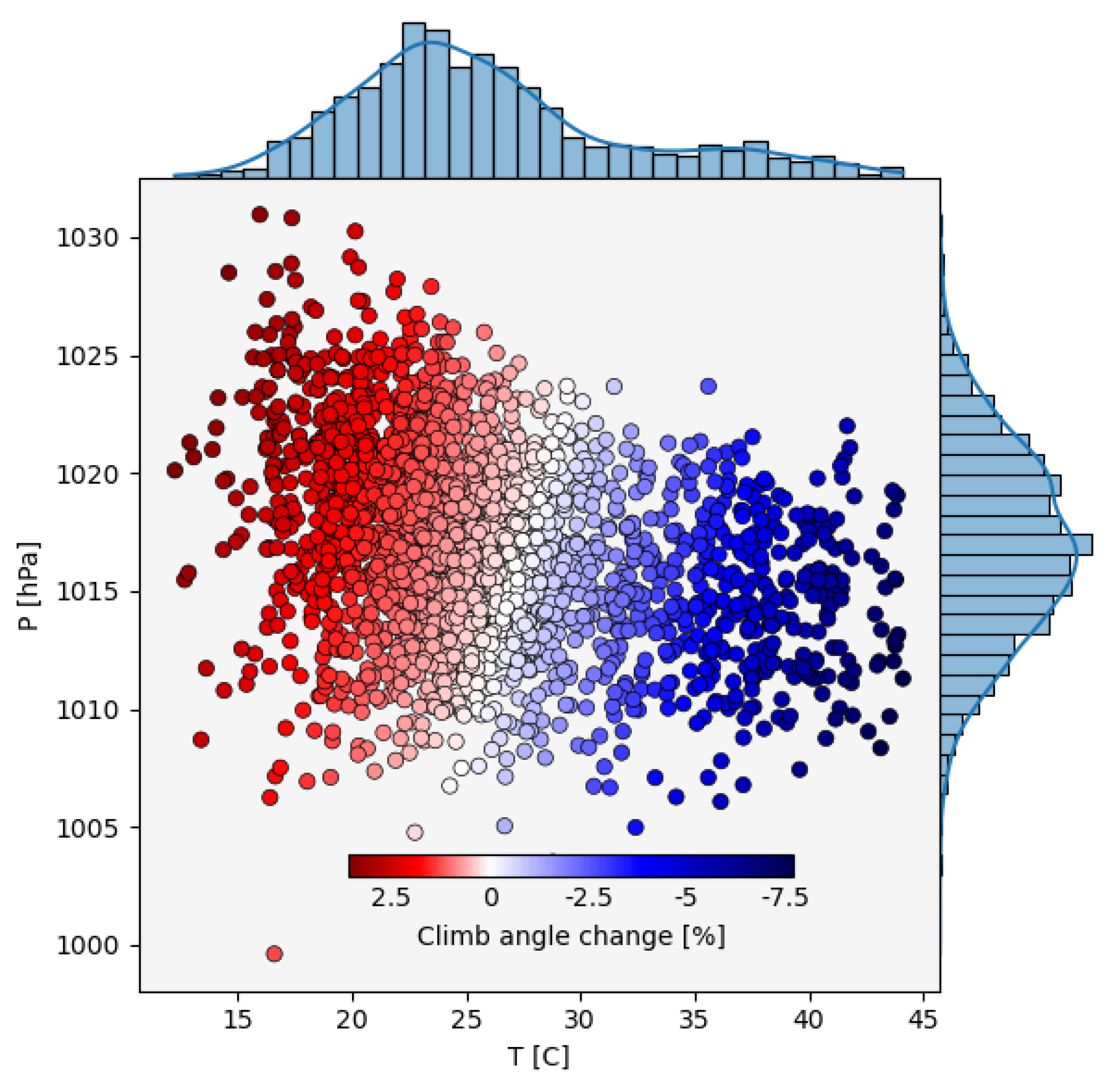
Figure 7.
Population densities at 30 arc second ( km) resolution for each of the study sites using WorldPop data [40]. The titles of each sub-figure show the ICAO airport code and the population density in the 3×3 km white dashed box centred on each airport’s location. The data for San Sebastian in sub-figure (p) is partially incomplete since this site is situated very near the French-Spanish border, although the airport itself lies in Spain, meaning that any estimates for this site in this work do not take the French population density into account.
Disclaimer/Publisher’s Note: The statements, opinions and data contained in all publications are solely those of the individual author(s) and contributor(s) and not of MDPI and/or the editor(s). MDPI and/or the editor(s) disclaim responsibility for any injury to people or property resulting from any ideas, methods, instructions or products referred to in the content. |
© 2025 by the authors. Licensee MDPI, Basel, Switzerland. This article is an open access article distributed under the terms and conditions of the Creative Commons Attribution (CC BY) license (http://creativecommons.org/licenses/by/4.0/).
Copyright: This open access article is published under a Creative Commons CC BY 4.0 license, which permit the free download, distribution, and reuse, provided that the author and preprint are cited in any reuse.


