Submitted:
16 June 2025
Posted:
17 June 2025
Read the latest preprint version here
Abstract
This paper outlines the considerations involved in designing an algorithm that can accurately and cost-effectively determine displacements for structural health monitoring, using standard image processing techniques and a convolutional neural network (CNN)-based object detection system. The algorithm can effectively identify and track geometric measurement motives across image sequences, enabling the precise determination of position and displacement. High levels of precision can be achieved through careful optimisation of geometric shape selection and pre-processing methods. A minimal example implementation using open-source, Python-based libraries demonstrates good agreement with reference measurements and minimal noise, highlighting the algorithm's potential. This flexible, robust approach offers substantial opportunities for further optimisation and application-specific scalability, making it a promising solution for structural health monitoring across various infrastructures.
Keywords:
SHM
; displacement measurement
; single camera system
; object detection
; low-cost
1. Introduction
Structural health monitoring (SHM) of infrastructure is becoming increasingly important. It is developing into an indispensable tool for ensuring the structural integrity of buildings [1,2,3]. In light of recent damage events such as bridge collapses, the continuous monitoring and analysis of the condition of structures is receiving increased attention in research and practice. Today’s infrastructure is exposed to numerous stress factors, including intensive use beyond its planned service life, increased heavy traffic, progressive ageing, and extreme weather events caused by climate change. Therefore, innovative solutions for SHM are essential to ensure the long-term safety of critical infrastructure. Alongside the well-established SHM methods, new approaches are becoming increasingly important. In this paper, we demonstrate the advantages of image-based measurement systems that use standard cameras. They are cost-effective, require simple cameras and sensors, and can operate under variable environmental conditions. Furthermore, this method can be used to retrofit existing monitoring systems, is minimally invasive, and can be operated using open-source software.
In general, systematic monitoring of structures, along with targeted repair measures based on this monitoring, significantly contributes to conserving resources. Such monitoring also plays a crucial role in preventing potential disasters [3,4]. In this context, measurement methods for detecting deformations and displacements are of particular scientific and practical interest. In addition to real-time monitoring, SHM offers the possibility of generating well-founded condition forecasts from the measured values. These forecasts can be used to optimize maintenance intervals and preventive maintenance measures [5,6]. As new construction methods and materials become more prevalent, the scalability of monitoring systems is becoming increasingly important through the integration of numerous distributed measuring points. This enables even complex and large-scale structures to be adequately monitored [7].
A variety of well-established methods exist for monitoring deformations and displacements in structures. These differ in terms of their measurement principles, accuracy and applicability [8,9,10,11]. Classic methods include strain gauges, which enable the direct and selective measurement of strains [12]. These sensors are widely used and offer high precision. However, they require direct access to the measurement point and can only be used in limited local areas [13]. Fibre optic sensors, particularly spatially resolved fibre optic systems, have become increasingly popular in recent years. They are particularly suitable for strain measurement over long distances and are insensitive to electromagnetic interference. While fibre Bragg grating sensors enable point measurements at defined locations along a fibre, distributed fibre optic sensors can provide continuous strain profiles over long distances. This allows both local and global deformations in complex structures to be detected [14]. Various types of displacement transducers are used to detect point displacements, including inductive, capacitive and potentiometric sensors [15]. These systems provide precise measurements at defined measurement points and are particularly suitable for monitoring critical areas. Laser sensors offer another option for detecting displacements. They detect changes in the position of a component by measuring the distance to a fixed reflector point [10]. Such systems are characterised by high measurement accuracy and contactless operation. However, they require a clear line of sight between the sensor and the reflector. In addition, image-based or camera-based measurement methods have become established. These methods offer flexibility and versatility in displacement detection [10,16,17]. They are often used to monitor the movement of entire building sections. Digital image correlation (DIC) can also be used to analyse surface deformations with high resolution [18]. These methods can detect both very small local changes and global movements. However, they require suitable image quality and stable environmental conditions. As each system has its own advantages and disadvantages, careful consideration must be given to the application, type of structure and measurement task. Therefore, the selection of the appropriate measurement method relies heavily on the specific requirements. The following factors are central to this decision: accuracy, measurement range, installation effort and environmental conditions [3].
Despite the wide range of measurement methods available, existing structural health monitoring (SHM) systems present technical and practical challenges that limit their widespread use [3,4]. A key problem is the high cost of complex measurement systems [4,19,20]. This is due to the costs of sensor technology and specialised hardware, such as interrogators and measurement amplifiers, as well as maintenance-intensive installations. The requirements for the measurement installation represent an additional hurdle. The application or integration of sensors and the laying and connection of cables—for example, the splicing of fibre optic sensors — requires technical expertise. Errors that impair measurement accuracy can occur during installation. Additionally, many systems only provide single measurements per sensor, which makes the comprehensive monitoring of large structures costly and technically challenging. Temperature and humidity fluctuations often need to be compensated to minimize measurement deviations, which makes data acquisition more complex. Dependence on proprietary evaluation software complicates interaction between different sensor systems, reduces flexibility in data analysis, and causes long-term costs due to reliance on a specific manufacturer [21]. Furthermore, many measurement methods are sensitive to mechanical influences and are not suitable for continuous use in harsh environments [22]. Power supply and data transmission are particularly challenging for wired systems. Cabling of large structures is logistically demanding and expensive [19,21].
As mentioned briefly at the beginning, the development of cost-effective, image-based measurement systems using standard cameras is a promising approach to solve the challenges above [23]. Single-camera systems offer the advantage of low acquisition costs. They also eliminate the need for proprietary measuring devices, because they allo the use of commercially available industrial cameras or modified single-lens reflex (SLR) cameras [23,24]. The system architecture allows flexibility in adapting to a wide variety of monitoring scenarios. Evaluation can be based on open-source algorithms and image processing methods [25]. A single camera can also be used to monitor several measurement positions simultaneously [26]. Specially developed measurement motives enable the precise detection of displacements in the range of sub-micrometres [24]. This method can detect various structural changes, from tilts to complex deformation patterns [11,27]. Open-source based data evaluation reduces dependence on specialised software and promotes transparent, adaptable analysis [28,29]. Machine learning methods that automatically extract features can further improve the accuracy of displacement measurements [30]. The combination of inexpensive hardware and scalable software architecture makes it possible to set up redundant measurement networks at low cost. These networks ensure reliable monitoring even under variable environmental conditions. This approach is minimally invasive: the measurement motives or markers can be attached to critical structural areas on a temporary or permanent basis, without requiring complex sensor integration into the building fabric. At the same time, the method allows existing monitoring systems to be retrofitted, enabling step-by-step integration into existing SHM systems.
This article examines the development and testing of an image-based, single-camera measurement system designed for two-dimensional displacement detection. The aim was to use a standard industrial camera and an appropriate measurement motive to accurately detect movements in two axes. A basic approach was followed that can be scaled as needed and adapted to different measurement situations. An algorithm was developed and evaluated using this approach in a minimal example with freely available open-source libraries. A linear table served as the reference system, causing displacements of the measurement motive. Thus, the linear table served as the measuring device. Laboratory tests revealed a high degree of agreement between the displacements determined by the camera and the reference values of the linear table. Based on the test results, opportunities for optimization and improvement, as well as challenges regarding SHM, are presented.
2. General Considerations
The following section outlines the key considerations for determining the position and displacement of measurement motives (MM) using a basic, single-camera system. This method can easily be scaled up, optimized, and implemented using open-source algorithms. This approach is based on four fundamental components:
- Pre-select ROIs based on object detection.
- ROI segmentation.
- Relative/absolute position determination.
- Displacement calculation.
Figure 1 shows the basic workflow. The considerations for each component are outlined below.
The order of the measurements depends on the design of the MM, which has two functions. Firstly, it determines the center of gravity, which establishes the position of the MM in the image. Secondly, it uses known geometric shapes to calculate the scale of the image in the measurement plane. This step is necessary in order to convert the displacement values obtained from the recorded pixel values into real distances.
The target should be designed so that the individual components can be segmented and assigned using standard image processing methods. There are generally no strict guidelines for this. However, it has proven useful to use simple geometric shapes such as circles, triangles, and rectangles, which can easily be distinguished from one another. In addition, double-symmetrical arrangements are preferable. The necessary size of the targets depends on the measurement task and the recording parameters, such as sensor size, lens, and measurement distance. The target´s relative size in the image section significantly affects the accuracy of the evaluation algorithm.
2.1. Pre-Select ROIs Based on Object Detection
Detecting MMs and geometric patterns in large image formats is challenging, especially when there are complex background configurations [31]. This is particularly true when it comes to identifying and differentiating between different, similar-looking MMs. However, SHM applications typically require the detection and classification of multiple MMs in large image sections with busy backgrounds. Therefore, this approach uses an object detection based on a CNN. This enables different motives to be detected and assigned simultaneously. A significant advantage of this approach is that, by using pre-selected regions of interest (ROI), processing can be performed only in selected areas. As a result, interference can be minimized and the required computing power can be reduced. A convolutional neural network (CNN) is a feed-forward controlled neural network that learns features independently through filter (or kernel) optimization. CNNs form the basis of deep learning algorithms in the AI subfield of machine learning, among others. Several CNN-based object recognition algorithms are available as open source libraries for common programming languages such as C or Python. The most popular algorithms currently are Faster R-CNN (Faster Region-Based Convolutional Neural Networks), SSD (Single Shot MultiBox Detector), and YOLO (You Only Look Once) [32]. Currently, YOLO appears to be the fastest and most reliable method, particularly for real-time applications [33]. However, the choice of object detection algorithm depends heavily on the specific application.
The approach described here is intended to support displacement measurement. For this purpose, efficiency in terms of processing speed and resource usage is particularly important. Thus far, it has not been possible to determine the center of the MM with sufficient precision for robust and accurate displacement measurements using only object detection algorithms. Therefore, the center of gravity of the MM has to be determined using other image processing methods. Nevertheless, object detection provides the ROI and important information for plausibility checks. Additionally, different MM designs can be linked to a database that stores information about the number and size of the geometric shapes they contain. These values are then used for further processing steps based on the recognised MM-ID. The following parameters are required as outputs:
- IDs of detected objects.
- Associated confidence scores.
- Coordinates of associated bounding boxes.
- Coordinates of associated centroids.
2.2. ROI Segmentation
The identified image sections (ROIs) must be pre-processed before any further analysis can be carried out. Edge detection prior to segmentation makes the latter easier and more accurate. The most well-known algorithms for this task were developed by Prewitt, Canny, and Sobel [34]. An important step in edge detection is to smooth the input image. This reduces noise and creates softer edge transitions. However, this can have both positive and negative effects. For instance, noise reduction minimizes the false detection of non-existent edges. Smoothing reduces discontinuities in pixel values along edges. Conversely, this can cause information to be lost. Therefore, it is important to tailor the smoothing functions to the application. Median, Gaussian, and bilateral filters are commonly used. Recommendations for selecting the appropriate edge detection algorithms, smoothing operations, and input parameters (e.g., kernel size) can be found in the extensive literature (e.g., [35,36,37,38,39]). The output of this step is the preselected areas (ROIs) of the overall image, presented as logical matrices.
In order to assign geometric elements to the MM, closed contours must first be determined in the edge detection logical matrices. Various approaches are described in the literature [40,41]. Most of these approaches follow the outer boundaries of closed series in logical matrices. Such algorithms can separate the shapes within the ROIs into individual elements. These elements can then be classified according to their geometric properties. In this context, it is advantageous to differentiate according to the number of corners. The most well-known corner detectors are the algorithms developed by Harris and Stephens [42,43] and the Shi-Tomasi algorithm [44]. For the purposes of this study, determining the number of corners is sufficient. Consequently, the preceding approaches provide adequate results. An exact determination of the corner position, as in the Förstner algorithm [45], is not required. Elements without corners, such as circles and ellipses, can be categorized based on circumference-to-area ratio or the Hough transform [46], among other methodologies. Once the contours have been determined and classified, additional information can be obtained, such as their surface areas and geometric centers.
This step involves performing a simultaneous plausibility check based on certain characteristics, such as the number of matched geometric shapes. This enables incorrect segmentations to be detected early on.
The following parameters must be transferred to the next processing step as output parameters:
- Recognized contours.
- Classification of contours into geometric elements.
- Geometric properties of the elements (e.g., coordinates of the geometric centers, surface area).
2.3. Relative/Absolute Position Determination
The results obtained can now be used to determine the position of each MM in relation to its respective ROI. There are various approaches available for this purpose. The simplest approach is to use the overall center of gravity of all the shapes that make up the MM. To improve accuracy or adapt the center of gravity determination to the application, only certain shapes can be used in the calculation. Other approaches can also be pursued, such as determining the center of gravity using different distances between individual centroids. The methodology largely depends on the MM design and the symmetry properties of the shapes’ arrangement. Since all approaches use averaged values from several centroids or distances, a resolution in the subpixel range can be achieved. The absolute positions of the MM centers can be determined using ROI coordinates in the overall image.
2.4. Displacement Calculation
Displacement is determined by comparing the positions of the MMs in different input images. The final step is to convert the relative displacements into physical units of length. First, the relationship between the optical image in the measurement plane and the actual size of the elements on the MM must be established. This requires the sizes of the geometric shapes to be known with high accuracy. One option is to calculate the ratio of the areas of certain or all elements. Alternatively, the distances between the centers or edges of the individual elements can be determined. Several approaches can lead to satisfactory results; therefore, optimization is always possible for individual measurement tasks. This step is crucial for accurate measurements. Even small inaccuracies can result in significant factorial measurement deviations. Finally, the target position at different times can be used as a reference value for a series of measurements across several images.
3. Experimental Investigations
To demonstrate the accuracy and scalability of the basic measurement algorithm described above, a minimal example was used for experimental investigations. The aim was to replicate the MM and the measurement algorithm using the most straightforward method possible.
3.1. Experimental Design
3.1.0.1. Measurement Motive
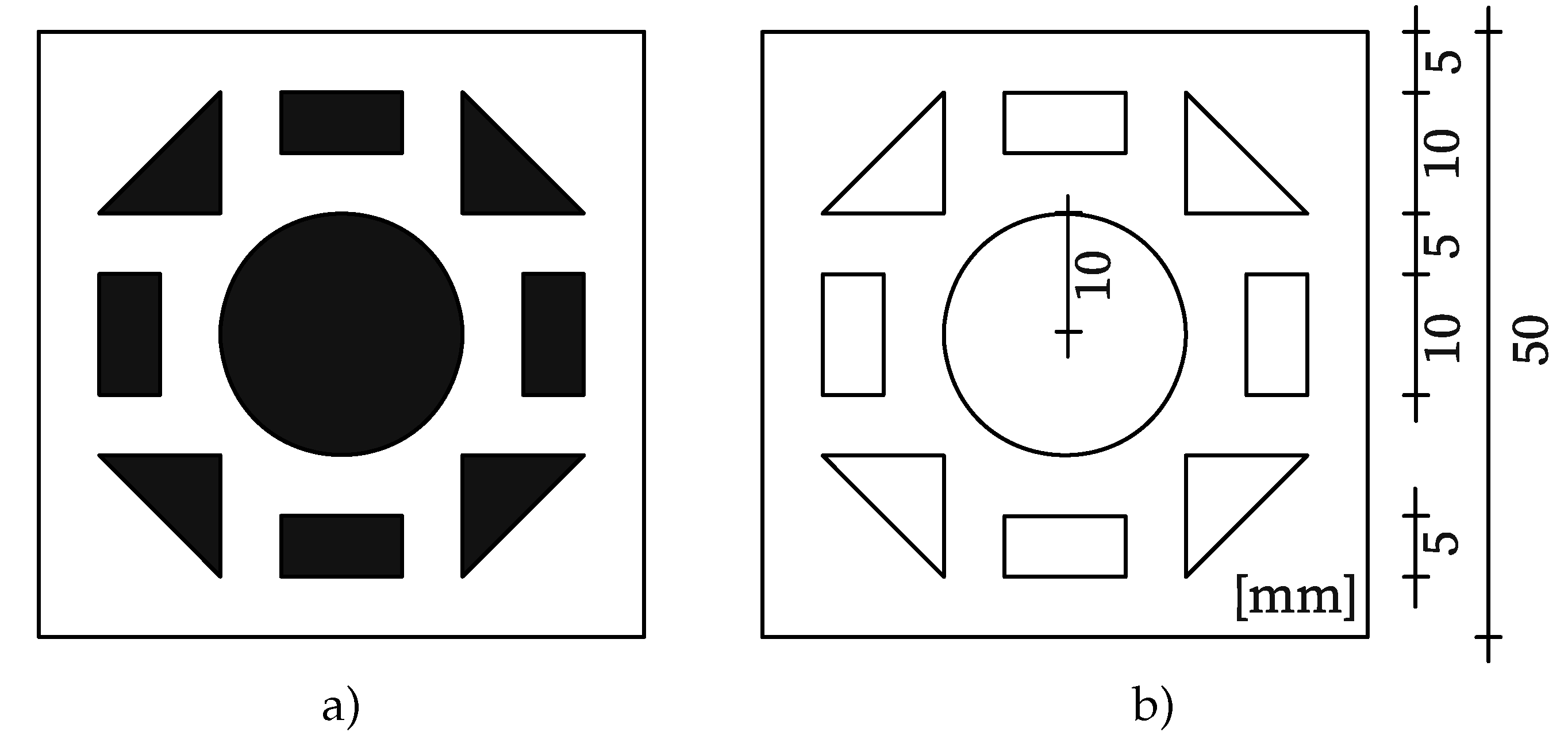
As part of the experimental investigations, a simple MM was developed and equipped with various geometric shapes. The different shapes were implemented to investigate how geometry, such as the number of corners or corner angles, influences the accuracy of the evaluation algorithm. The chosen arrangement was a symmetrical pattern of right-angled isosceles triangles and rectangles with an aspect ratio of 2:1 and a centrally located circle (see Figure 2). For the test, the MM was printed on a 4 thick aluminum Dibond panel and attached to the linear stage using an aluminum angle bracket.
The object’s overall dimensions are 50 50. The rectangles have edge lengths of 10 5, and the triangles have side lengths of 10. The circle in the center has a radius of 10.
3.1.0.2. Test Setup
The test setup consists of a rigid frame made from aluminum system profiles. The camera is mounted on one side using a bracket made of 15 thick steel plates. On the other side there is a linear stage on which the MM is mounted with an aluminum bracket. The distance between the camera and the MM is 2.35. LED spotlights are mounted symmetrically at a distance of 0.87 from the test object. They are adjusted to illuminate the test object with an illuminance of 800 at a color temperature of 4400. The entire frame is vibration-isolated using six steel isolator springs and elastomeric bearings. The setup is located in an controlled room with a constant temperature of 20 ∘C and a relative humidity of 65. Figure 3 shows a schematic of the frame setup:
For the experimental investigations, a monochrome industrial camera with a 2/3-inch sensor (Basler A2A4200-12gmBAS) was used. The lens used was a 2/3-inch lens with a fixed focal length of 50 and an aperture range of F2.8 - F16.0 (Basler C23-5028-5M-P). The camera sensor (GMAX2509) provides a maximum resolution of 4200 2160 pixels with a maximum pixel bit depth of 12 bits and a pixel size of 2.52.5.
The linear stage used has a bidirectional repeatability of 0.8 and is equipped with a linear encoder with a resolution of 80. Due to the high accuracy of the internal measurement system, the linear encoder readings were used as the position reference for this test. A stepped travel regime with five steps of 1.5 in the positive and negative direction was selected. The holding times are 170 each and the total test time is 60. Figure 4 shows the travel path of the test sequence as recorded by the linear encoder of the stage.
A separate recorder synchronously recorded both the camera images and the linear encoder readings every 5.
3.2. Minimal Implementation of the Algorithm
In order to verify the functionality with a minimal example, an algorithm was developed that implements the functions described in Section 2. This algorithm developed is based entirely on Python and uses the following libraries:
- ultralytics (8.3.99)
- torch (2.6.0+cu126)
- opencv-python (4.10.0.84)
- numpy (1.26.4)
The individual components and functions of the algorithm are described below.
3.2.0.3. CNN Object Detection
The real-time object detector from the YOLO series (Generation 11) was used for object detection. This CNN algorithm from Ultralytics is licensed under AGPL 3.0, allowing free non-commercial use. A dataset comprising 253 images was created to train the model, depicting various constellations with and without the MM to be detected. This dataset was divided into 222 training images and 31 validation images. The model used in the example was trained with the pretrained model “YOLO11l”, which is based on the COCO dataset. 200 epochs were used, and the target image size was 1024 pixels.
3.2.0.4. ROI Segmentation
Only the ROI determined for the object identifier was used for further processing. Therefore, the subsequent steps relate to a small area of the image. This significantly improves the performance of the functions. Due to the MM’s illumination and the high resolution of the camera sensor, this approach used a median filter (OpenCV function medianBlur()) with a 5 x 5 pixel window size. Next, edge detection was performed on the image section using the Canny algorithm (OpenCV function Canny()). Threshold values of 100 and 200 were set for the gradient.
The findContours() function from OpenCV, based on [47], was used for contour detection. The contour retrieval algorithm was set to `RETR_EXTERNAL’, which only considers outer contour points. The approximation algorithm was set to `CHAIN_APPROX_NONE’, which preserves all contour points. This function returns a nested array of individual closed contours. These arrays can then be iterated to classify the contours:
- General
- To ignore contours incorrectly detected due to noise, a query was performed considering only contours with a minimum area of 100 pixels. The threshold value should be chosen carefully based on the expected minimum sizes of the geometric shapes.
- Circles
- First, to classify circles, the circumference (P) and area (A) of the contour must be determined. Then, circularity [48], an auxiliary variable, is defined as a parameter. The formula is as follows: . A perfect circle has a circularity of 1. A threshold value can be defined for classification depending on the desired tolerance. In this case, the threshold value was set to 0.85, as this yielded the best results with the setup shown; shapes with values above this threshold are considered circular.
- Polygons
- The OpenCV contour approximation algorithm was used to classify the triangles. The approxPolyDP() function implements the Ramer-Douglas-Peucker algorithm [49,50], which reduces a curve consisting of line segments to a similar curve with fewer points. In this case, the approximation accuracy was defined as 10% of the perimeter. The number of corners can be determined based on the number of remaining approximated lines, which are output as individual arrays. Depending on the chosen approximation accuracy, this algorithm is highly robust. However, for certain applications, other corner detection algorithms may be preferable.
Additionally, the centroids were determined for each classified contour using the image moments of the individual arrays. As part of a plausibility check, the number of shapes in each category was compared (one circle, four triangles, and four rectangles).
Relative/Absolute Position Determination
Two methods were used to determine the overall center of gravity in the MM. Firstly, the arithmetic mean of all the shapes’ centroids was calculated. Secondly, the calculation was performed separately for each shape. Using the ROI coordinates, the relative coordinates of the center of gravity can be converted to an absolute position within the image.
Image Scale Determination and Displacement Measurement
Three approaches were used to determine the image scale:
- Area
- The easiest way to determine the image scale is to compare the actual size of the geometric shapes on the MM to the size of the enclosed area of the classified contours: .
- Circles
- Circular shapes can be compared based on their circle parameters, such as radius, circumference, or area. In this case, the radius was determined using the OpenCV function minEnclosingCircle() on contours classified as circles. The actual radius is 10.
- Polygons
- In the third approach, the image scaling is determined by comparing the distances between the individual centroid points of the triangles and rectangles. The distances between the centers of gravity of the triangles are 26.667 mm between adjacent elements and 37.712 mm between opposite elements. For the rectangles, the distances are 24.749 mm between adjacent elements and 35 between opposite elements. The overall values for beta were determined using the mean values of all the respective shape ratios.
Finally, the displacements are determined by comparing the MM positions of several images and converting them into real units using the image scaling factor.
Results
Object Detection
Object detection yielded satisfactory results across the entire dataset, achieving an average confidence value of 0.899. However, the quality of object detection varies slightly depending on the position of the measurement target (see Figure ).
Filtering and Edge Detection
Figure 6 illustrates the ROI of the detected MM, for which edge detection was performed on the initial measurement image. The median filter produces smooth contours and reduces noise. However, clear corners are lost, and small roundings form.
Segmentation
The quality of the segmentation remained consistently reliable throughout the entire dataset. The correct number of closed contours could be determined in each image and categorized as geometric figures. The plausibility check yielded positive results for all measurements, indicating that the correct number of circle, triangle and rectangle elements were identified in each case. Therefore, the threshold value for corner detection appears to be within a satisfactory range. Figure 7 shows the array of the overall image with the segmented geometric elements in the MM.
Determination of Motive Position
The centers of the geometric shapes can be determined using the image moments of the contour elements. Figure 8 shows the categorized shapes and their respective centers of gravity for the first image in the set.
These centers of gravity are then used to determine the overall center of gravity. There are several methods of achieving this. One method is to calculate the overall center of gravity as the arithmetic mean of the individual centroids of the geometric shapes. Alternatively, different combinations and weightings of the centers of gravity of the individual geometric shapes can be used (e.g., circles and rectangles only).
Figure 9 shows a comparison of the centers of gravity calculated from each shape category during the measurement period before the first displacement step. Overall, the level of noise in the subpixel range is low. There are differences between the calculated centers of gravity of the individual geometric elements. While the circle and rectangle values differ only slightly, the triangle values deviate more significantly. These differences shift the arithmetic mean of all elements. However, triangles exhibit the lowest level of noise.
Determination of the Image Scale and Displacement Measurement
The image scale was determined using several methods to convert the displacement values into physical units of measurement. First, the total area of the recognized geometric elements was compared with the actual area present on the MM. Additionally, the image scale was determined using the diameter of the individual circular element. Lastly, it was determined based on the distances between the centroids of the rectangles and triangles. Figure 10 shows the image scales determined for the entire dataset. The methods used to determine the total area and circle diameters show significant deviation from the well-correlated values obtained using center point distances.
This suggests that preprocessing with a median filter and edge detection resulted in a loss of significant information. Consequently, the determined edge deviates from the actual course, resulting in inaccurate size comparisons. However, since this information loss is consistent across all edges, it has a minimal impact on the center of gravity of the elements, especially for double-symmetrical shapes, such as rectangles. Figure 11 shows the comparison of the calculated displacements in the X direction for the first five steps using different approaches. First, the position determination and image scale calculation were conducted solely on the circles. Second, these values were determined using the corresponding centroids of the individual triangle or rectangle elements.
Displacement values determined using only rectangles correlate best with the reference values. This results in a high degree of agreement, especially in areas with small displacements. Values determined using triangles show that the degree of agreement with the reference values varies with displacement. This indicates a factorial issue related to the determined image scale factor (see Figure 12).
Figure 12 shows the absolute deviations of the measurements determined using triangles. This figure shows all measurement points along the entire displacement path.
The factorial error is clearly visible here. Overall, the measurement’s accuracy is only moderate. However, the measured values vary very little on specific displacement steps, resulting in low measurement uncertainty (see Figure 13). As expected, the uncertainty of the measurements increases with displacement.
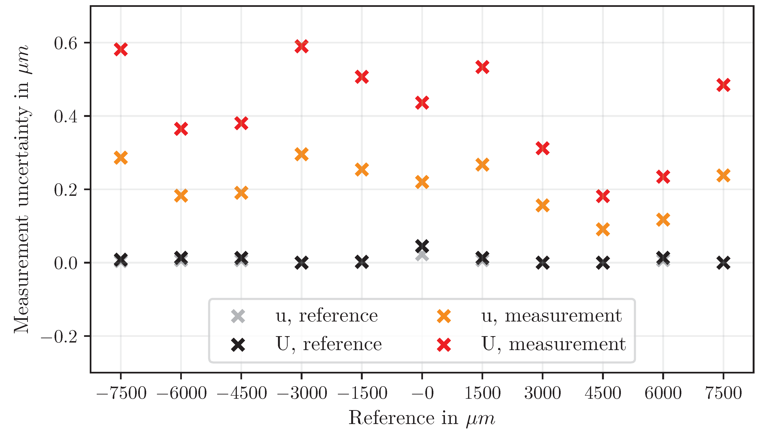
In contrast, the measured values obtained using the rectangles exhibit significantly smaller deviations (see Figure 14).
Even with large displacement ranges, the comparison shows good agreement, with deviations of less than 10 in most cases. The dispersion shows similar values across all displacement ranges. Overall, the extended measurement uncertainty is less than 0.6 (see Figure 15).
Discussion
Overall, the experimental investigations show promising results. Object detection achieved high confidence values even with a relatively small training dataset and recognized the MMs reliably. The slight differences in confidence values are probably due to the limited training data and depend on the position of the measurement markers. Nevertheless, these differences play a minor role and do not affect subsequent processing steps. Subsequent work steps are limited to the cut-out ROIs for object recognition. This allows a significantly more robust measurement of the motives. Edge detection of the ROIs enabled reliable contour detection of the geometric shapes. However, information loss occurs in the form of rounded corners and shifted edges. This is usually caused by using blur filters in the preprocessing step for edge detection. In the example implementation, two filters were initially used: One was a median filter with a 5 x 5 kernel, and the other was the Gaussian filter contained in the cv.Canny() function from OpenCV, also with a 5 x 5 kernel. These filters enabled edge detection with minimal noise, smooth lines, and few outliers. Nevertheless, the use of both filters should be viewed critically. In particular, the center of gravity shifts in non-bilaterally symmetrical shapes. This does not significantly affect position determination in bilaterally symmetrical MMs because similar information losses occur in all shapes, resulting in an average. However, significant effects occur when determining the image scale, for example. Firstly, the total area of the enclosed contours changes. Secondly, the shift in the center of gravity influences the center of gravity distance ratios. The choice of filters for edge detection generally depends on the lighting (e.g., reflections, illuminance), the quality of the image sensor and lens, and the print quality of the MM. This choice should be carefully considered in relation to the specific application.
As shown in Figure , there are only minor differences in the determination of the MM’s absolute position within the image. These differences range from 0.3 pixels in the X direction, corresponding to approximately 34 based on the determined image scale. In the Y direction, the differences are smaller, reaching a maximum of 23. Therefore, the geometric properties of the individual components of the MM, at least in a double symmetrical arrangement, appear to have only a minor effect on positional accuracy. However, the difference between circular and rectangular shapes compared to triangular elements is somewhat notable. While the loss of information at the corners and edges of triangles leads to lower noise in position determination, it distorts the actual center of gravity ratios.
Even though the geometric shape of the elements in the MM plays a minor role in determining position, it plays a significant role in determining the image scale. As shown in Figure 10, deviations of up to 4.5/pixel can occur. These deviations significantly influence the displacement measurements because they have a factorial effect on the measured variable. Figure 11 illustrates this clearly: displacement measurements based on rectangles are presumably inaccurate in terms of position determination, whereas displacement measurements based on triangles and circles show a dependence of deviation on the displacement path. Therefore, determining the image scale is critical for absolute displacement measurements, particularly for large displacements.
In this case, the method that takes the rectangles (double-symmetrical) into account is the most appropriate way to determine the displacements. This method produced the best results and showed a high degree of agreement with the reference. The absolute deviations shown in Figure 14 are limited to a range of 10. This level of accuracy is sufficient for most applications. Additionally, the measured values of the individual steps (forward and return) exhibit only minor deviations, with extended measurement uncertainties of less than 1. As this is a minimal example, there is significant potential for optimization and application-specific scalability. Significantly better accuracies can be achieved through careful implementation of the measuring principle and optimization of the individual functions and motive design.
Conclusions
This paper presents a proposal for a simple algorithm to measure the displacement of targets using basic cameras. This involves using CNN object detection to identify and assign targets. The targets are then measured using standard image processing methods, enabling position determination and displacement measurement across image series.
To demonstrate the algorithm, its considerations were translated into concrete functions in a minimal example using open-source Python-based libaries, and an experimental test program was carried out. The results of the investigation are promising: even the minimal example achieves good agreement with the reference and exhibits only slight noise. During the investigations, the suitability of different geometric shapes for the MM was also evaluated. It was found that both a double-symmetrical arrangement of the shapes and double-symmetrical geometries of the individual elements deliver the best results. Overall, the algorithm still offers enormous potential for increased accuracy and functionality. Thanks to the use of open-source libraries, the individual components and functions can be scaled and optimized as required for specific applications. Furthermore, additional functions can be added. For instance, parameters such as the tilt or rotation of the measurement motives can be determined (e.g. based on the size ratios of opposing elements within the MM).
Author Contributions
DM and MW conceptualized the algorithm, performed the experiments, evaluated the data in relation to the topic, and wrote the final paper. KH accompanied the experiments and provided advice on the conceptual design of the paper. All authors read and approved the final paper.
Data Availability Statement
The datasets used and analyzed in the current study are available from the corresponding author upon reasonable request.
Conflicts of Interest
The author declare that they have no conflict of interest.
References
- Nithin, T.A. Real-time structural health monitoring: An innovative approach to ensuring the durability and safety of structures. 11, 43. [CrossRef]
- Brownjohn, J. Structural health monitoring of civil infrastructure. 365, 589–622. [CrossRef]
- Aktan, E.; Bartoli, I.; Glišić, B.; Rainieri, C. Lessons from Bridge Structural Health Monitoring (SHM) and Their Implications for the Development of Cyber-Physical Systems. 9, 30. [CrossRef]
- Farrar, C.R.; Worden, K. An introduction to structural health monitoring. 365, 303–315. [CrossRef]
- Rabi, R.R.; Vailati, M.; Monti, G. Effectiveness of Vibration-Based Techniques for Damage Localization and Lifetime Prediction in Structural Health Monitoring of Bridges: A Comprehensive Review. 14, 1183. [CrossRef]
- Anjum, A.; Hrairi, M.; Aabid, A.; Yatim, N.; Ali, M. Civil Structural Health Monitoring and Machine Learning: A Comprehensive Review. 18, 43–59. [CrossRef]
- Laflamme, S.; Ubertini, F.; Di Matteo, A.; Pirrotta, A.; Perry, M.; Fu, Y.; Li, J.; Wang, H.; Hoang, T.; Glisic, B.; et al. Roadmap on measurement technologies for next generation structural health monitoring systems. 34, 093001. [CrossRef]
- Gharehbaghi, V.R.; Noroozinejad Farsangi, E.; Noori, M.; Yang, T.Y.; Li, S.; Nguyen, A.; Málaga-Chuquitaype, C.; Gardoni, P.; Mirjalili, S. A Critical Review on Structural Health Monitoring: Definitions, Methods, and Perspectives. 29, 2235. [Google Scholar] [CrossRef]
- Hassani, S.; Dackermann, U. A Systematic Review of Optimization Algorithms for Structural Health Monitoring and Optimal Sensor Placement. 23, 3293. [CrossRef]
- Kot, P.; Muradov, M.; Gkantou, M.; Kamaris, G.S.; Hashim, K.; Yeboah, D. Recent Advancements in Non-Destructive Testing Techniques for Structural Health Monitoring. 11, 2750. [CrossRef]
- Palma, P.; Steiger, R. Structural health monitoring of timber structures – Review of available methods and case studies. 248, 118528. [CrossRef]
- dos Reis, J.; Oliveira Costa, C.; Sá da Costa, J. Strain gauges debonding fault detection for structural health monitoring. 25, e2264. [CrossRef]
- Bolandi, H.; Lajnef, N.; Jiao, P.; Barri, K.; Hasni, H.; Alavi, A.H. A Novel Data Reduction Approach for Structural Health Monitoring Systems. 19, 4823. [CrossRef]
- Weisbrich, M.; Holschemacher, K.; Bier, T. Comparison of different fiber coatings for distributed strain measurement in cementitious matrices. 9, 189–197. [CrossRef]
- Scuro, C.; Lamonaca, F.; Porzio, S.; Milani, G.; Olivito, R. Internet of Things (IoT) for masonry structural health monitoring (SHM): Overview and examples of innovative systems. 290, 123092. [CrossRef]
- Kim, J.W.; Choi, H.W.; Kim, S.K.; Na, W.S. Review of Image-Processing-Based Technology for Structural Health Monitoring of Civil Infrastructures. 10, 93. [CrossRef]
- Dong, C.Z.; Catbas, F.N. A review of computer vision–based structural health monitoring at local and global levels. 20, 692–743. [CrossRef]
- Boursier Niutta, C.; Tridello, A.; Ciardiello, R.; Paolino, D.S. Strain Measurement with Optic Fibers for Structural Health Monitoring of Woven Composites: Comparison with Strain Gauges and Digital Image Correlation Measurements. 23, 9794. [CrossRef]
- Morgenthal, G.; Eick, J.F.; Rau, S.; Taraben, J. Wireless Sensor Networks Composed of Standard Microcomputers and Smartphones for Applications in Structural Health Monitoring. 19, 2070. [CrossRef]
- Mustapha, S.; Lu, Y.; Ng, C.T.; Malinowski, P. Sensor Networks for Structures Health Monitoring: Placement, Implementations, and Challenges—A Review. 4, 551–585. [CrossRef]
- Malik, H.; Khattak, K.S.; Wiqar, T.; Khan, Z.H.; Altamimi, A.B. Low Cost Internet of Things Platform for Structural Health Monitoring. In Proceedings of the 2019 22nd International Multitopic Conference (INMIC). IEEE. [Google Scholar] [CrossRef]
- Kralovec, C.; Schagerl, M. Review of Structural Health Monitoring Methods Regarding a Multi-Sensor Approach for Damage Assessment of Metal and Composite Structures. 20, 826. [CrossRef]
- Sony, S.; Laventure, S.; Sadhu, A. A literature review of next-generation smart sensing technology in structural health monitoring. 26, e2321. [CrossRef]
- Feng, D.; Feng, M.; Ozer, E.; Fukuda, Y. A Vision-Based Sensor for Noncontact Structural Displacement Measurement. 15, 1657. [Google Scholar] [CrossRef]
- Henke, K.; Pawlowski, R.; Schregle, P.; Winter, S. Use of digital image processing in the monitoring of deformations in building structures. 5, 141–152. [CrossRef]
- Ye, X.W.; Dong, C.Z.; Liu, T. A Review of Machine Vision-Based Structural Health Monitoring: Methodologies and Applications. 2016, 1–10. [CrossRef]
- Feng, D.; Feng, M.Q. Experimental validation of cost-effective vision-based structural health monitoring. 88, 199–211. [CrossRef]
- Chen, B.; Tomizuka, M. OpenSHM: Open Architecture Design of Structural Health Monitoring Software in Wireless Sensor Nodes. In Proceedings of the 2008 IEEE/ASME International Conference on Mechtronic and Embedded Systems and Applications. IEEE; pp. 19–24. [CrossRef]
- Basto, C.; Pela, L.; Chacan, R. Open-source digital technologies for low-cost monitoring of historical constructions. 25, 31–40. [CrossRef]
- Xu, Q.; Wang, X.; Yan, F.; Zeng, Z. , Non-Contact Extensometer Deformation Detection via Deep Learning and Edge Feature Analysis. In Design Studies and Intelligence Engineering; IOS Press. [CrossRef]
- Peters, J.F. Foundations of Computer Vision. [CrossRef]
- Aboyomi, D.D.; Daniel, C. A Comparative Analysis of Modern Object Detection Algorithms: YOLO vs. SSD vs. Faster R-CNN. 8, 96–106. [CrossRef]
- Bilous, N.; Malko, V.; Frohme, M.; Nechyporenko, A. Comparison of CNN-Based Architectures for Detection of Different Object Classes. 5, 2320. [Google Scholar] [CrossRef]
- Kumari, R.; Chandra, D. Real-time Comparison of Performance Analysis of Various Edge Detection Techniques Based on Imagery Data. 42. [CrossRef]
- Li, P.; Wang, H.; Yu, M.; Li, Y. Overview of Image Smoothing Algorithms. 1883. [CrossRef]
- Chen, B.H.; Tseng, Y.S.; Yin, J.L. Gaussian-Adaptive Bilateral Filter. 27, 1674. [Google Scholar] [CrossRef]
- Shreyamsha Kumar, B.K. Image denoising based on gaussian/bilateral filter and its method noise thresholding. 7, 1172. [Google Scholar] [CrossRef]
- Das, S. Comparison of Various Edge Detection Technique. 9. [CrossRef]
- Magnier, B.; Abdulrahman, H.; Montesinos, P. A Review of Supervised Edge Detection Evaluation Methods and an Objective Comparison of Filtering Gradient Computations Using Hysteresis Thresholds. 4. [CrossRef]
- Yang, D.; Peng, B.; Al-Huda, Z.; Malik, A.; Zhai, D. An overview of edge and object contour detection. 488. [CrossRef]
- Papari, G.; Petkov, N. Edge and line oriented contour detection: State of the art. 29. [CrossRef]
- Harris, C.; Stephens, M. A Combined Corner and Edge Detector. pp. 23.1–23.6. [CrossRef]
- Sánchez, J.; Monzón, N.; Salgado, A. An Analysis and Implementation of the Harris Corner Detector. 8. [CrossRef]
- Shi, J. ; Tomasi. Good features to track. pp. 593–600. [CrossRef]
- Förstner, W.; Gülch, E. A Fast Operator for Detection and Precise Location of Distict Point, Corners and Centres of Circular Features.
- Illingworth, J.; Kittler, J. The Adaptive Hough Transform. PAMI-9. [CrossRef]
- Suzuki, S.; be, K. Topological structural analysis of digitized binary images by border following. 30. [CrossRef]
- Montero, R.S.; Bribiesca, E. State of the Art of Compactness and Circularity Measures. 2009.
- Ramer, U. An iterative procedure for the polygonal approximation of plane curves. 1. [CrossRef]
- Douglas, D.H.; Peucker, T.K. Algorithms for the Reduction of the Number of Points Required to Represent a Digitized Line or its Caricature. pp. 15–28. [CrossRef]
Figure 1.
Basic workflow.
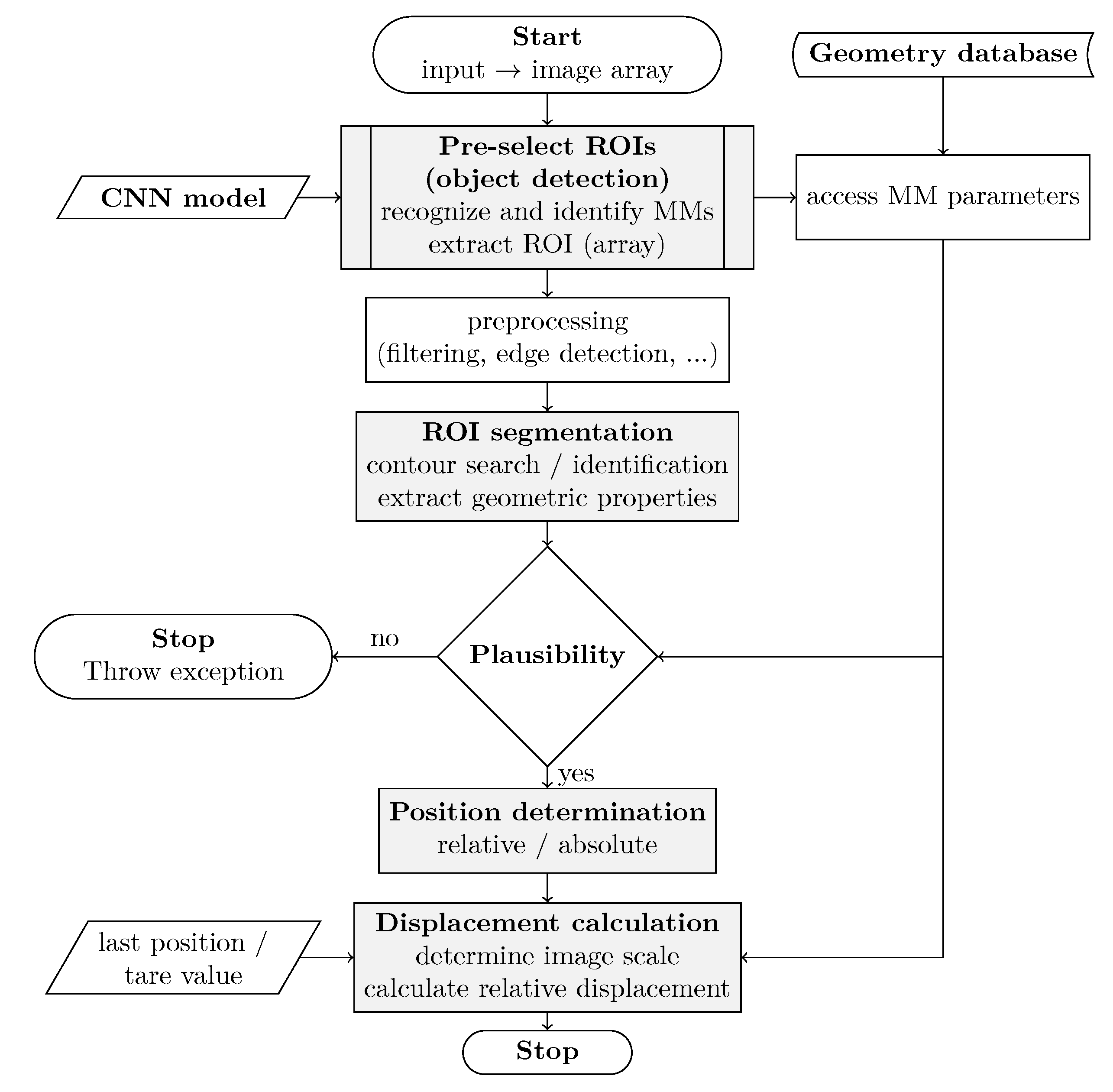
Figure 2.
a) Measurement motive (MM), b) dimensioned representation of the MM.
| a) | b) |
Figure 3.
Schematic test setup.
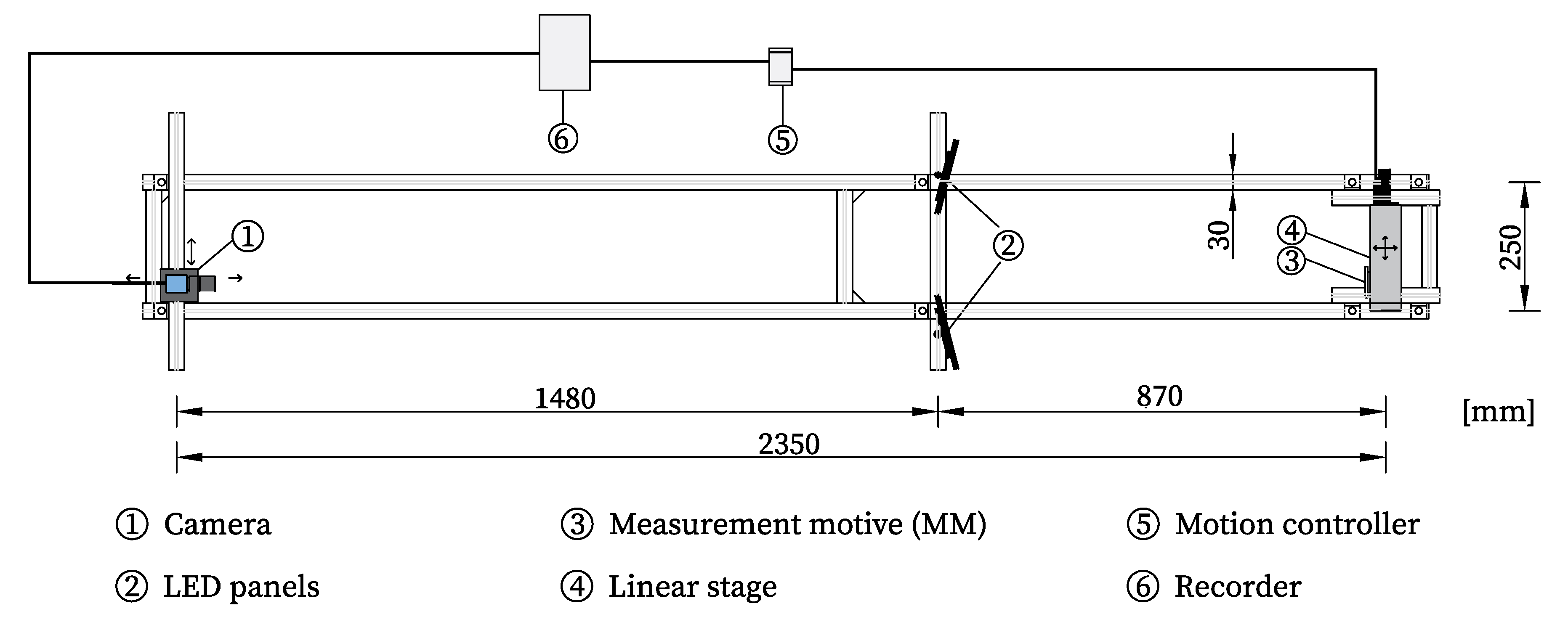
Figure 4.
Displacement path.
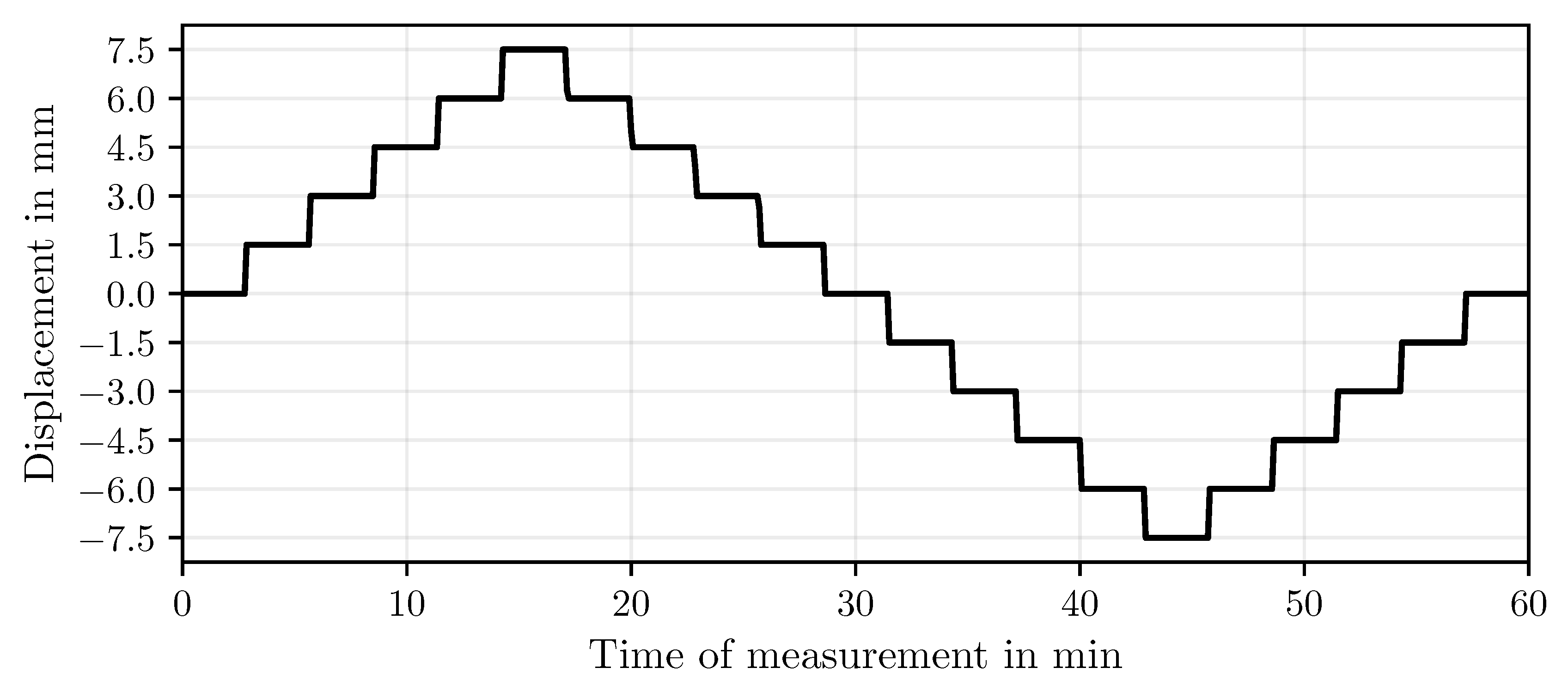
Figure 5.
Confidence scores of YOLO object detection.
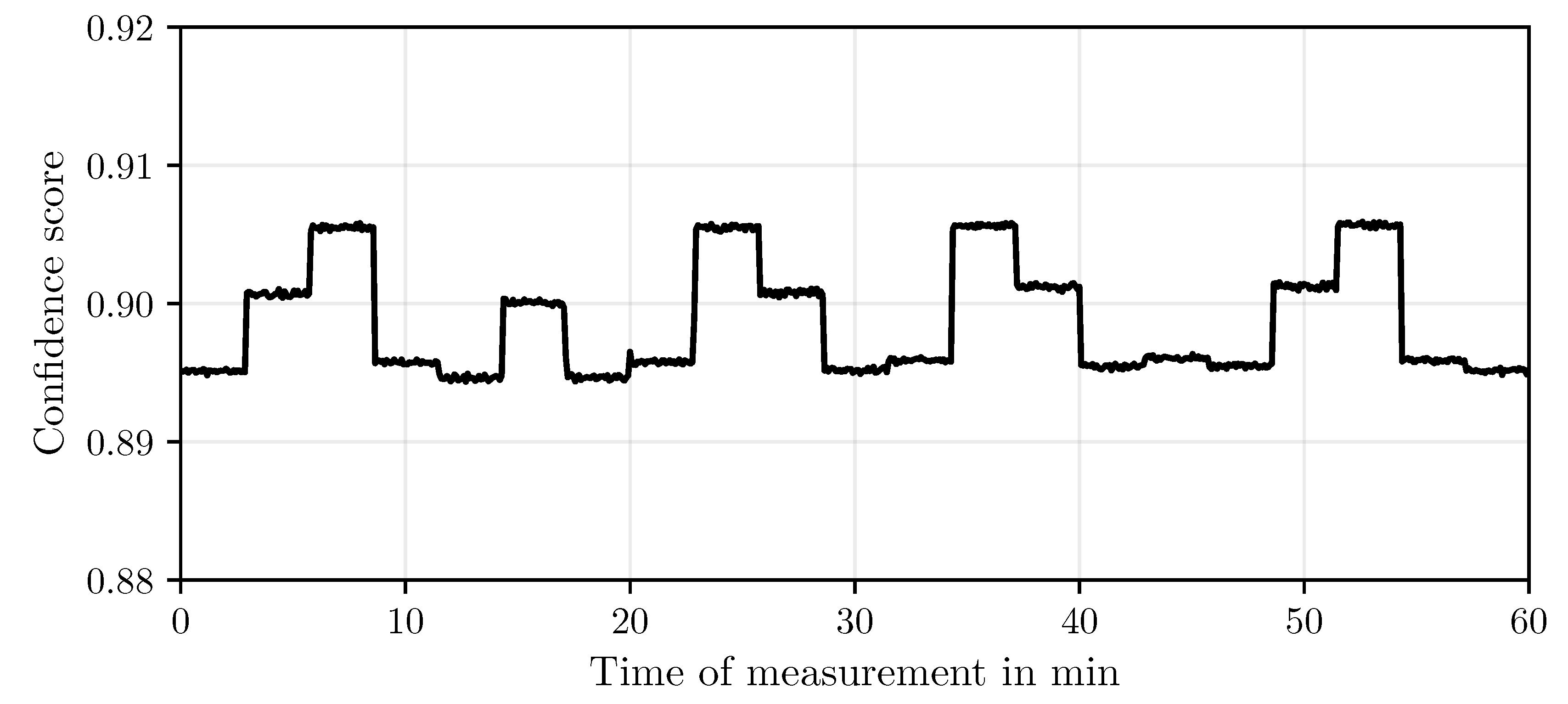
Figure 6.
Cut out ROI with detected edges.
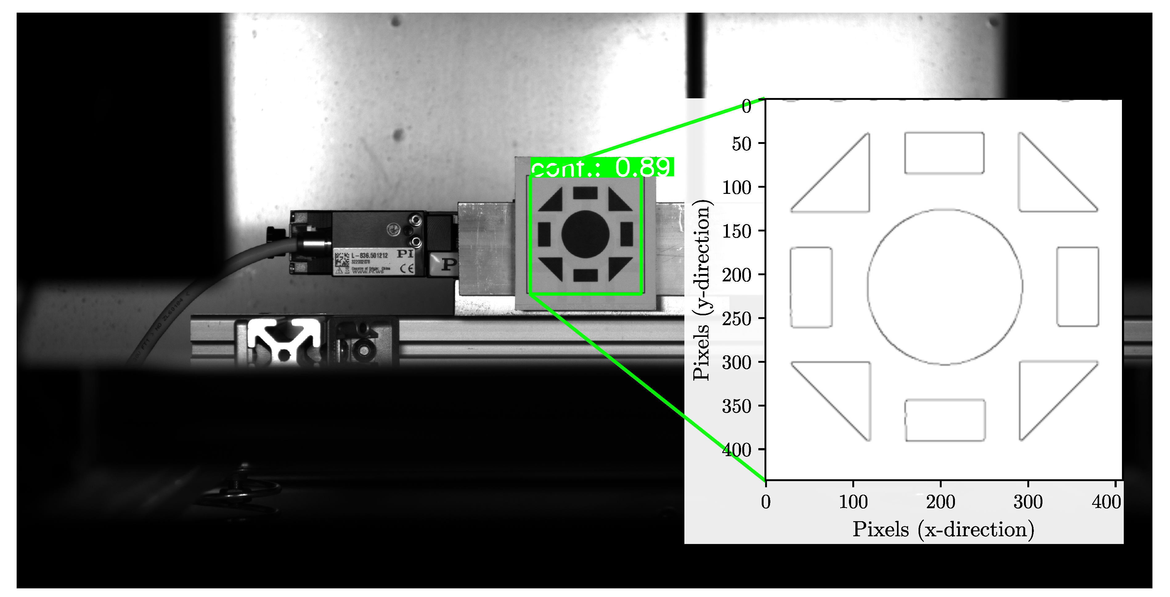
Figure 7.
Segmentation.
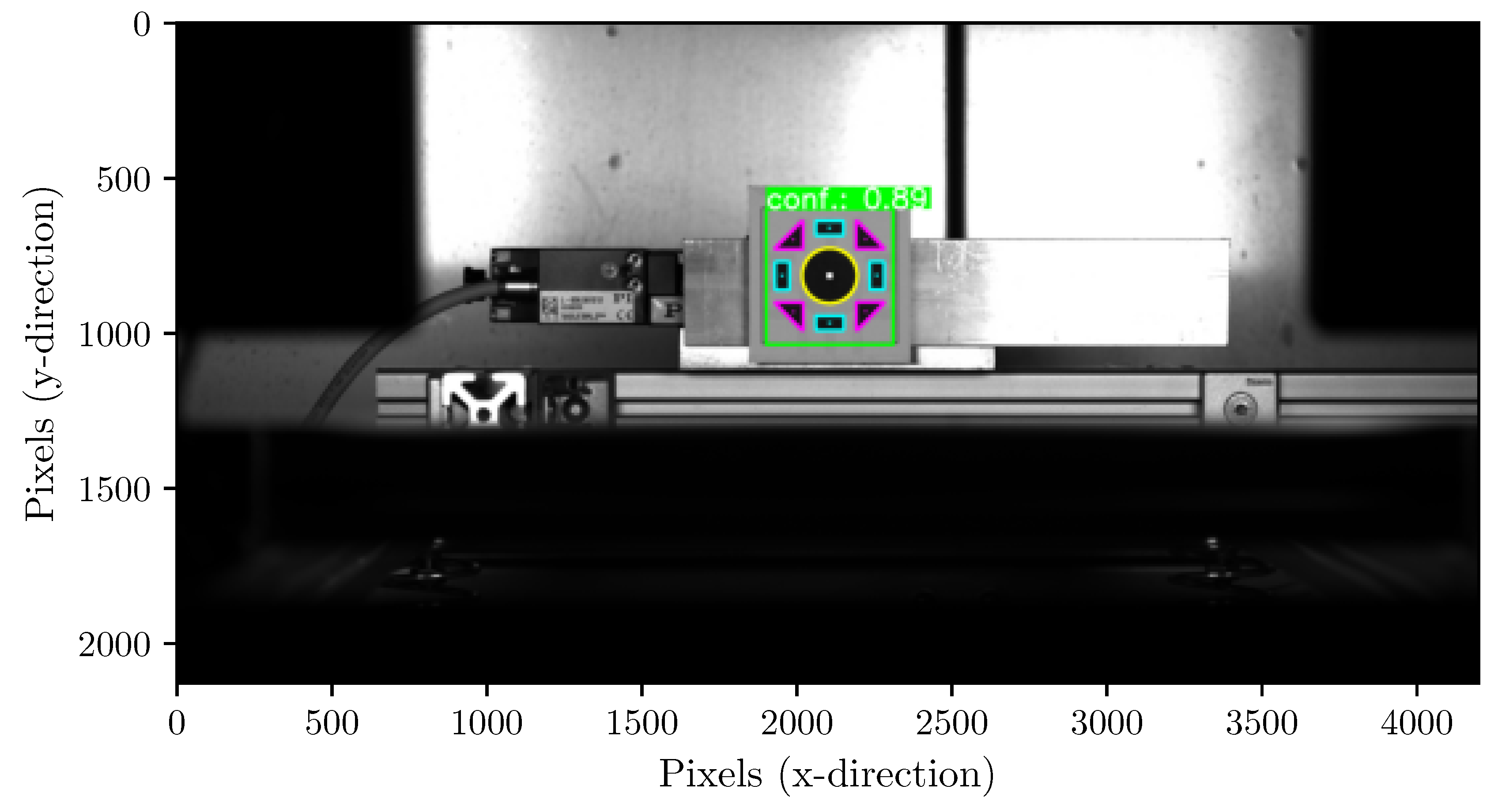
Figure 8.
Centroids of the geometric shapes in the cropped ROI.
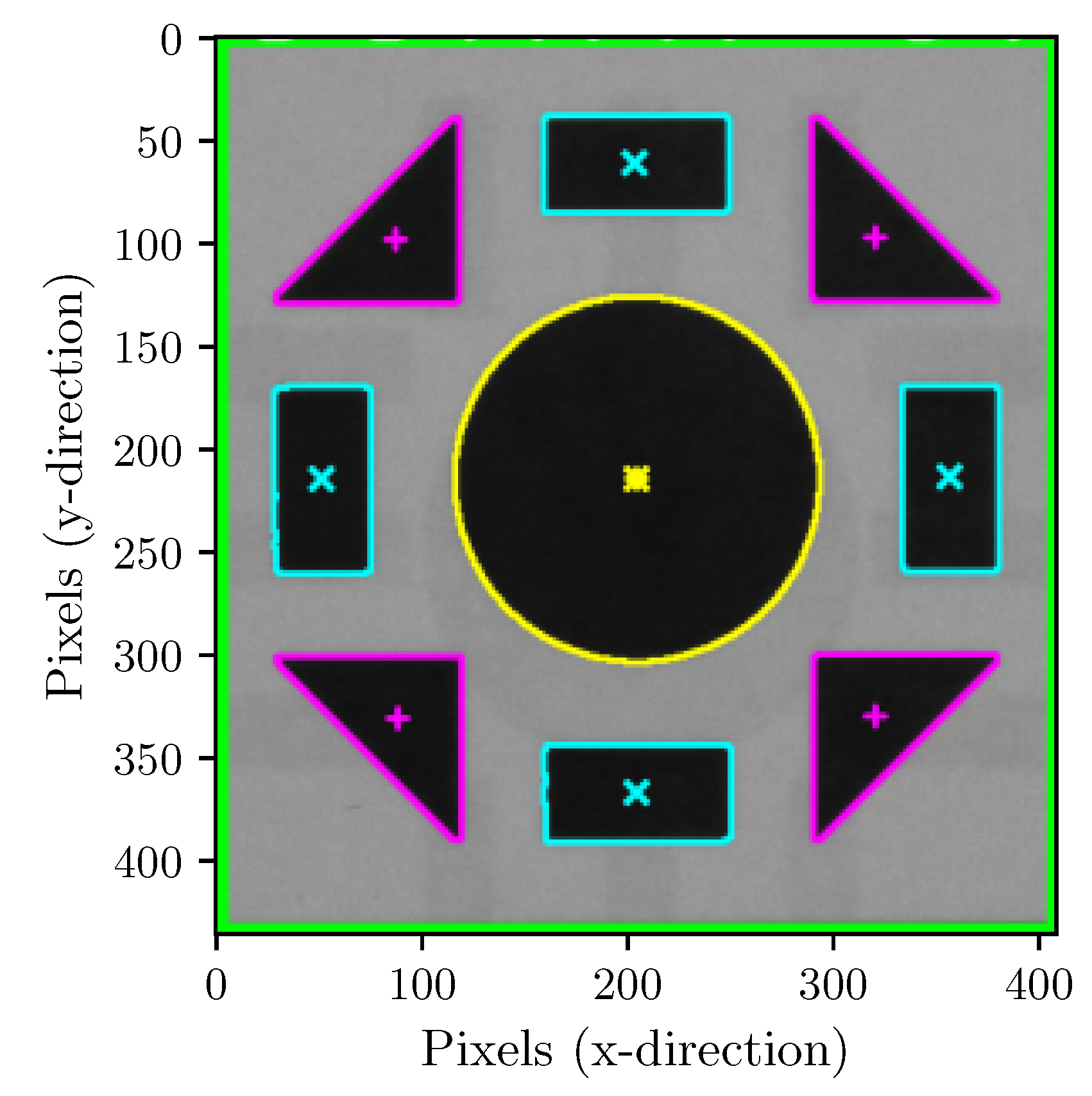
Figure 9.
Absolute centroid position of the target.
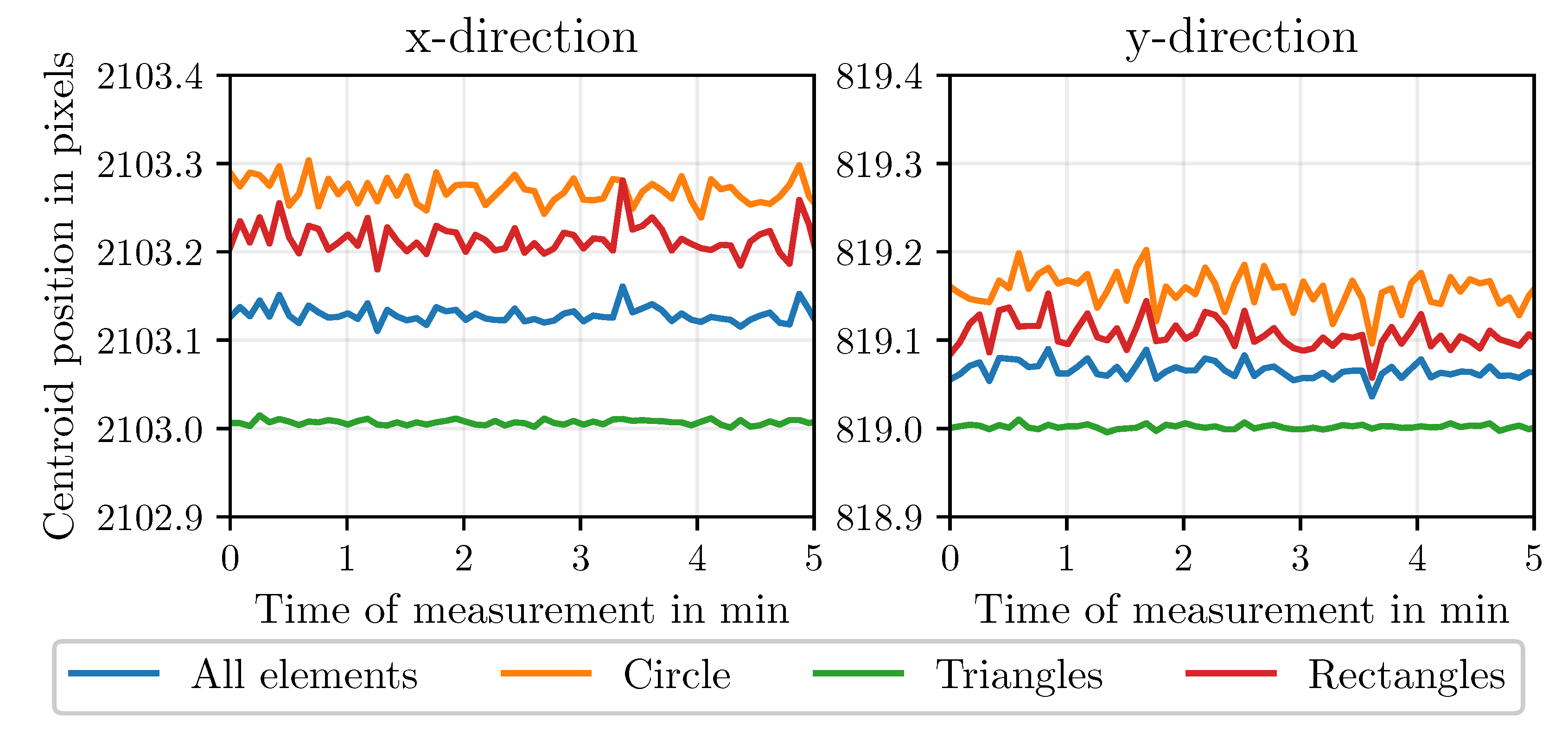
Figure 10.
Comparison of methods for determining the image scale.
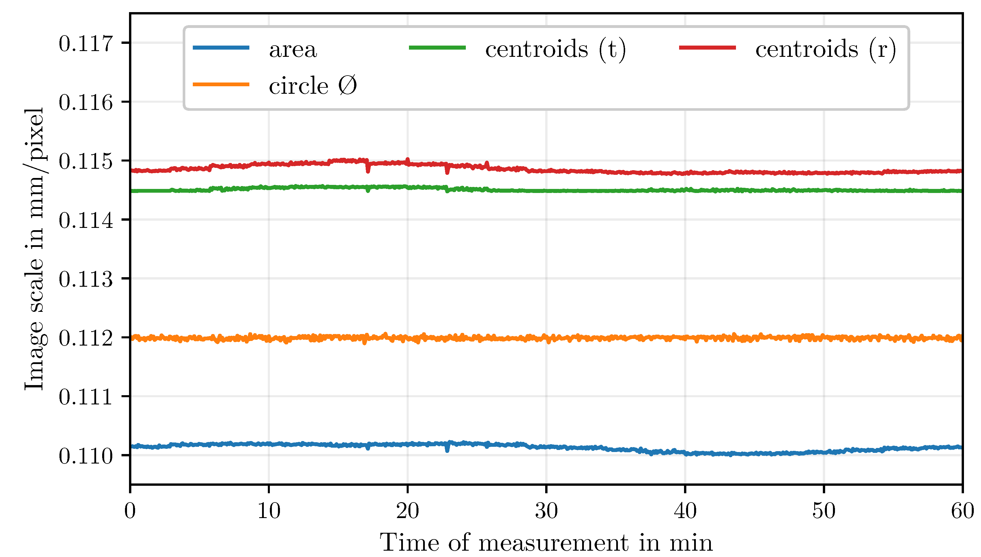
Figure 11.
Comparison of displacement calculation using different methods.
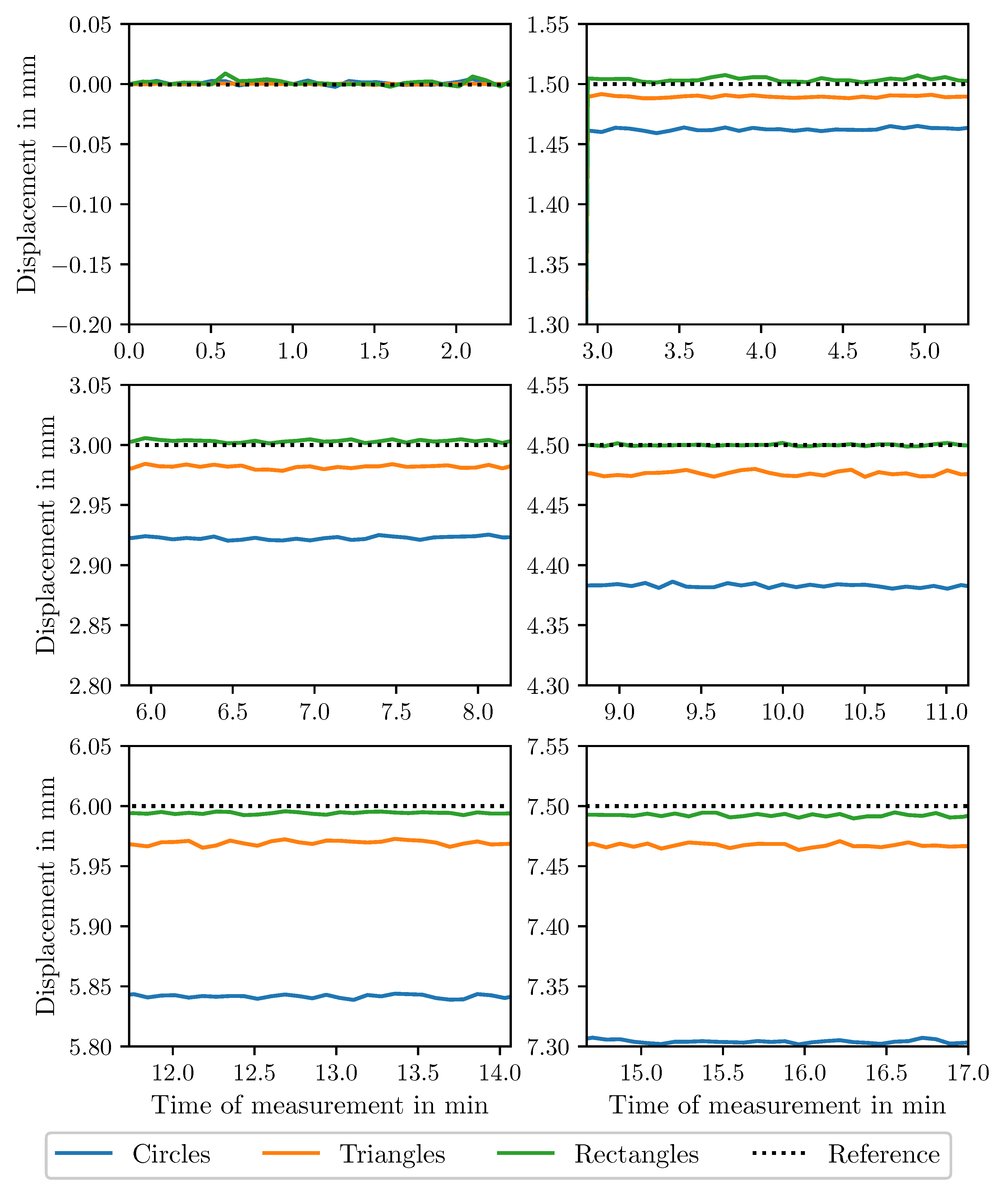
Figure 12.
Absolute deviations of the measurements determined using triangles.
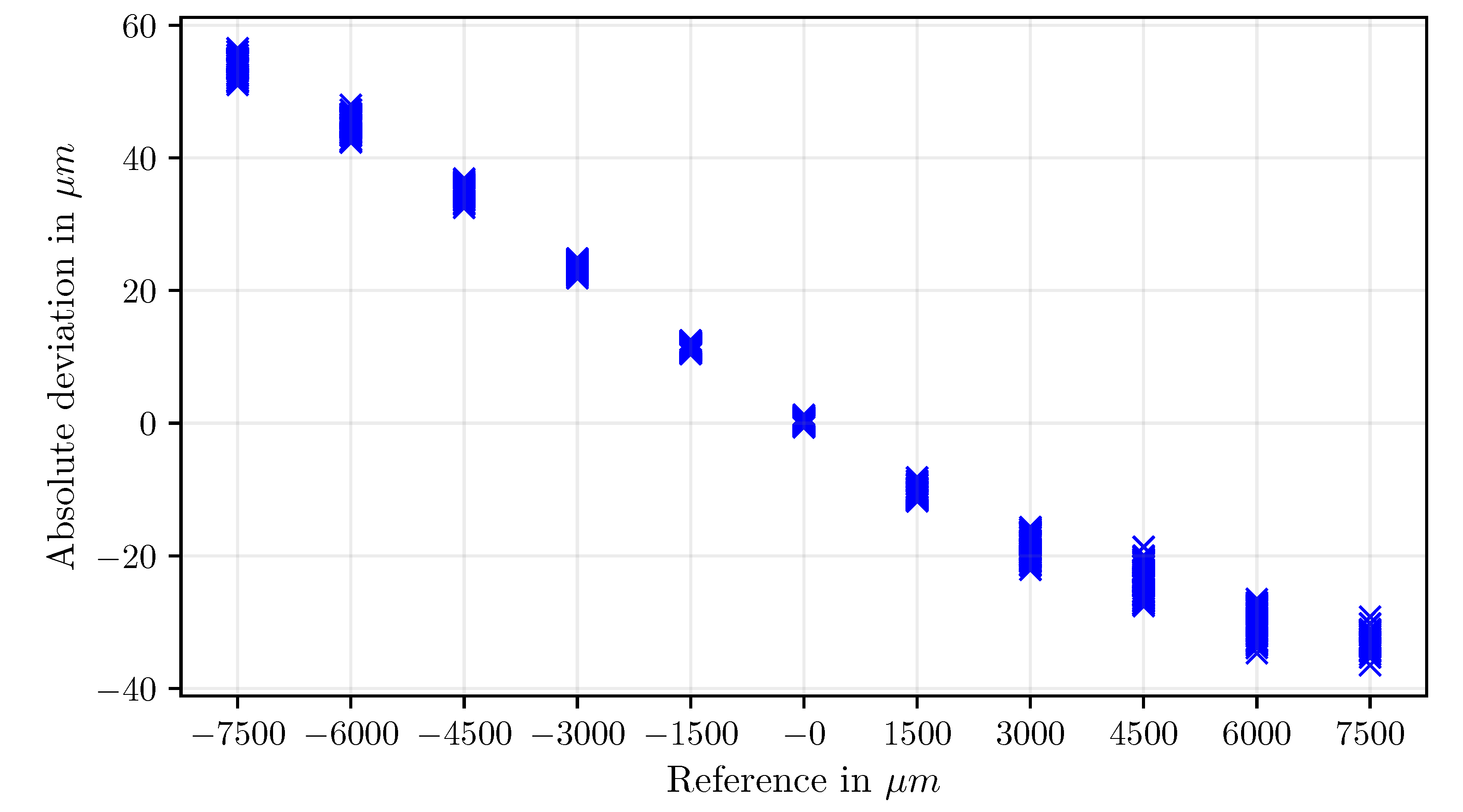
Figure 13.
Measurement uncertainty of the values determined using triangles.
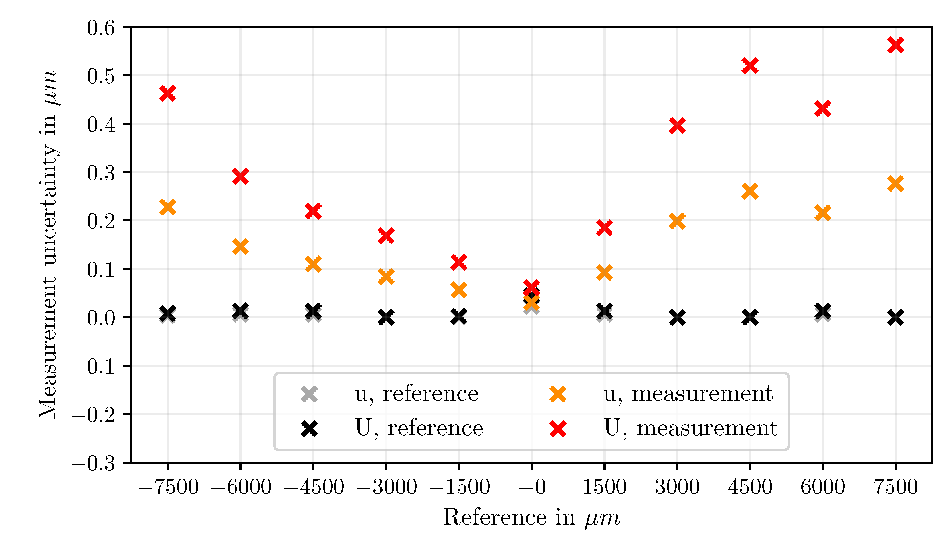
Figure 14.
Absolute deviations of the measurements determined using rectangles.
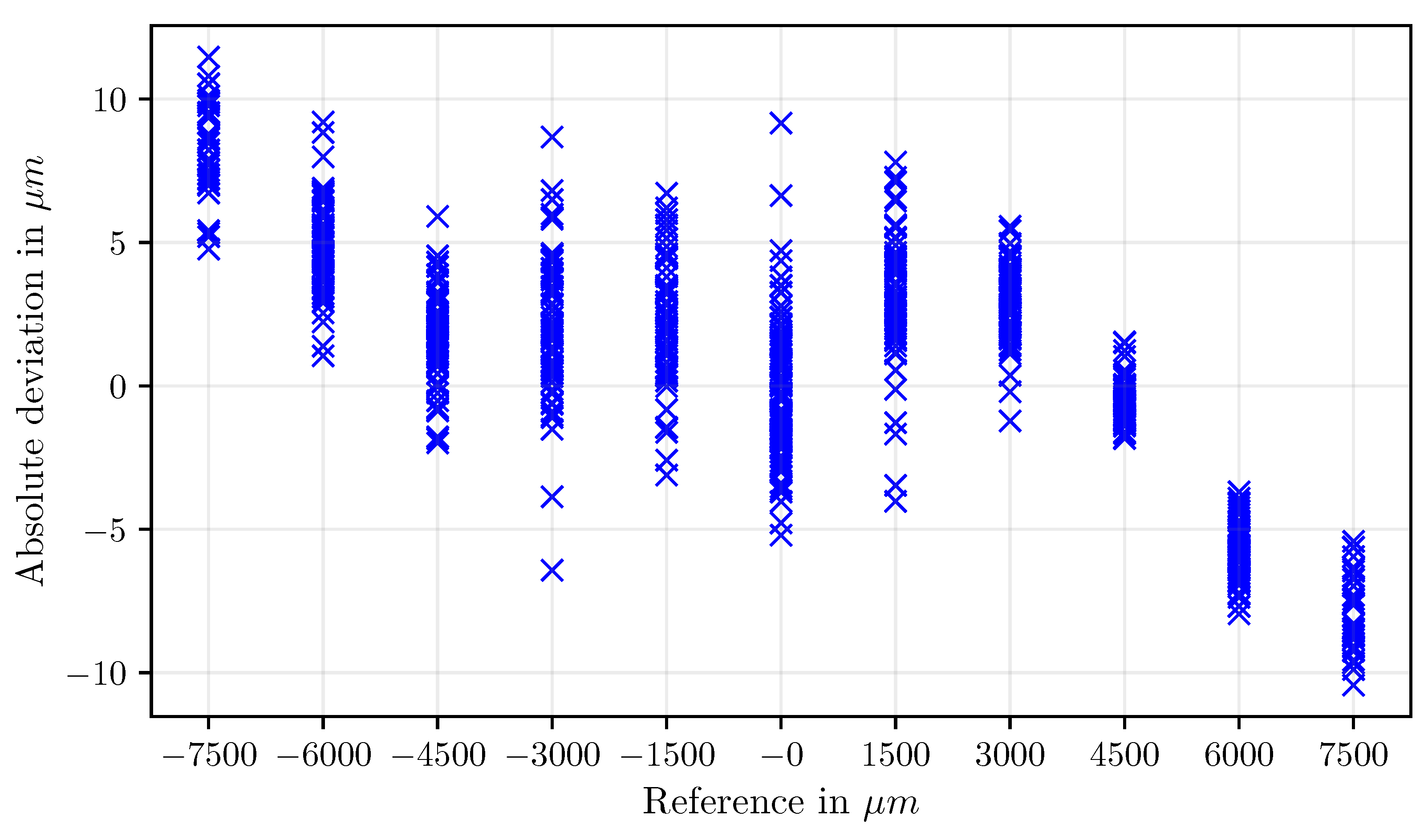
Figure 15.
Measurement uncertainty of the values determined using rectangles.
Disclaimer/Publisher’s Note: The statements, opinions and data contained in all publications are solely those of the individual author(s) and contributor(s) and not of MDPI and/or the editor(s). MDPI and/or the editor(s) disclaim responsibility for any injury to people or property resulting from any ideas, methods, instructions or products referred to in the content. |
© 2025 by the authors. Licensee MDPI, Basel, Switzerland. This article is an open access article distributed under the terms and conditions of the Creative Commons Attribution (CC BY) license (http://creativecommons.org/licenses/by/4.0/).
Copyright: This open access article is published under a Creative Commons CC BY 4.0 license, which permit the free download, distribution, and reuse, provided that the author and preprint are cited in any reuse.


