
Submitted:
15 June 2025
Posted:
16 June 2025
You are already at the latest version
Abstract
The new generation of robots (Industry 5.0 and beyond) is expected to be accompanied by the massive introduction of autonomous and cooperative agents in our society, both in the industrial and service sectors. Cooperation with humans will be simplified by humanoid robots with a similar kinematic outline and a similar kinematic redundancy, which is required by the diversity of tasks that will be performed. A bio-inspired approach is proposed for coordinating the redundant DOFs of such agents. This approach is based on the ideomotor theory of action, combined with the passive motion paradigm, to implicitly address the degrees of freedom problem, without any kinematic inversion, while producing coordinated motor patterns structured according to the typical features of biological motion. At the same time, since the approach is force-field-based, it allows us to integrate in the computational loop parallel modules that exploit the redundancy of the system for satisfying geometric or kinematic constraints implemented by appropriate repulsive force fields. Moreover, the model is expanded to include dynamic constraints associated with the Lagrangian dynamics of the humanoid robot to improve the energetic efficiency of the generated actions.
Keywords:
Cognitive robotics
; Neural simulation of action
; Prospection
; Passive Motion Paradigm
; Generative Body Schema
; Degrees of freedom problem
1. Introduction
Humanoid robots share with humans the issue of how to deal with the redundancy of a complex, articulated body for the coordination of purposive actions. The first researcher to address the problem scientifically was probably Nikolai Bernstein [1], who observed the performance of professional workers in repetitive tasks, as hammering blacksmiths, and found that precise hammer trajectories across repetitive trials were produced by highly variable rotation patterns of the redundant set of joints recruited for the task. From such observations Bernstein [2] formulated the general problem of motor redundancy, to be solved by the worker’s brain, observing that the motor system must produce many more control signals than the variables that characterize and constrain typical skilled actions, and proposed that the solution consists in the elimination of redundant degrees of freedom, allowing the brain to focus only on the essential elements.
The issue of motor redundancy, focused on the problem of how to coordinate the excessive number of DoFs (Degrees of Freedom), is intertwided with the empirical evidence that human multi-joint movements are charachterized by spatio-temporal invariants of the motion of the end-effector, whatever the number of recruited DoFs, such as the bell-shaped speed profile in reaching movements [3] or the anticorrelation of the speed and curvature profiles in general gestures of the hand, as in cursive handwriting [4,5]. As a matter of fact, the spatio-temporal invariances express the smoothness of biological motion in general full-body actions [6]. They can be explained by the minimum jerk model [7], in the framework of a remarkable feature of energetic frugality of biological motion, which has been demonstrated in human motor control [8] as well as in industrial robotics [9].
The general rationale of the smoothness of biological motion in connection with the emergence of figural-kinematic invariances can be linked to the ideomotor theory, already formulated by psychologists of the 19th century, as William James [10] and recently reviewed with more solid neurophysiological support [11,12]. According to this theory, the brain of a skilled person initiates the computational process that will lead to the performance of a purposive action by formulating the idea of the relevant sensory consequences (as the expected trajectory of the end-effector) rather than the detailed coordination of the DoFs recruited for the actual execution of the action and the corresponding muscle activation patterns. Shortly, an action idea mediates between the intention to act and the generation of detailed motor control patterns. The problem is how to express computationally such a process that requires facing the broad imbalance between the numerosity of the DoFs of the body and the number of parameters that characterize the action idea. Such an imbalance is already high in the human case. Still, it pales compared with other species such as the elephant trunk and the octopus tentacles, i.e., muscular hydrostats with infinite DoFs. On the other hand, it is remarkable that the invariant features of the elephant’s purposive actions [13] are quite similar to those of human biological motion.
The approaches developed to deal with DoF imbalance reveal a wide range of opposite evaluations. For example, some researchers designate it (negatively) as redundancy [14], whereas others [15] describe it (positively) as motor abundance, emphasizing a basket of affordances that includes flexibility and adaptability to various ancillary aspects of skilled behavior.
The issue of kinematic redundancy in robotic manipulators is well established and formulated mainly as a problem of inverse kinematics. This is a complex problem, in contrast with direct kinematics (the mapping of joint rotation patterns into the corresponding law of motion of different body parts, i.e., different end-effectors): direct kinematics is a well-defined problem with a unique solution, whichever the number of DoFs, whereas inverse kinematics is an ill-posed problem which may involve infinite solutions or no solution at all. The number of methods proposed in robotics is very large. Most focus on the Jacobian matrix, with various forms of pseudo-inversion whose computational robustness decreases with the increase of the degree of redundancy of the robot architecture, as in humanoid robots. In particular, many proposals are based on the null space projection technique developed in the 1980s [16,17,18]. However, most robotic redundancy resolution schemes do not allow integration of the inverse kinematic process with the issue of smoothness, typical of biological motion, or the various constraints that the coordinated joint rotation patterns are supposed to satisfy, as the range of motion of the DoFs, the range of torque of the actuators, or the range of stability in bipedal standing.
The proposed approach is bio-inspired, in the general sense that it is built upon the recognition of the already cited bliss of motor abundance, articulated in such a way to include the basic elements of the ideomotor theory and the intrinsic smoothness of biological motion, integrated with the capability of multiple constraint satisfaction. The main module is a computational model, named Passive Motion Paradigm (PM) [19,20,21], which is based on the Jacobian matrix of the body schema, as in many robotic formulations, but without any attempt to invert it or explicit utilization of the associated null space. The basic concept, implicit in the ideomotor theory, is to shift the focus from primitive motions to primitive force fields: this means that if our brain is requested to carry out the ill-posed task of coordinating the multiple DoFs of the body in order to “push” the end-effector towards a designated target, it may instead imagine to “pull” the end-effector to the target and then the body will follow, i.e., the whole kinematic chain will passively yield to the pulling field thus producing a coordinate rotation pattern of the redundant DoFs. This is equivalent to using the transpose Jacobian for mapping a pulling force field, defined in the low-dimensional task space, into an equivalent torque field, operating in the high-dimensional joint space. The “passivity” of the planning paradigm is modulated by a compliance matrix that maps the torque field into incremental joint rotations and then, via the same Jacobian matrix, into the incremental motion of the end-effector, attracted to the target according to the ideomotor theory by an attractive force field.
The attractive dynamics of the PMP can be integrated with the repulsive dynamics of additional modules which express geometric or structural constraints, as the RoM (limited Range of Motion) of the different DoFs or the constraint of bipedal stability that implies a RoM of the position of the center of mass of the body on the support area. Such constraints can generate online repulsive torque fields combined additively with the attractive torque field for a coordinated synergy formation process that implicitly exploits the null space for a trade-off between the competing requirements of the different modules. In this paper, the PMP approach to motor redundancy is extended with the motor adaptation of the compliance matrix related to a number of other dynamic constraints involving the torque requirements of the different actuators.
2. Methods
The proposed model of coordination of the redundant DoFs of full-body robots is illustrated in Figure 1. The top panel is the general block diagram built around the PMP (Passive Motion Paradigm) module, which implements the ideomotor theory, in parallel with two blocks which implement geometric and kinematic constraints to be satisfied on-line during the simulation of the model for driving the full-body synergy formation process: (a) the CoM constraint for the postural stability of the standing robot, i.e., the requirement of constraining the projection of the CoM (Center of Mass) inside the convex hull of the support area between the feet, and (b) the RoM constraint, for the structural integrity of the body model, i.e., the requirement to keep the rotation angle of each DoF inside the Range of Motion of each joint. Additional blocks can be integrated to express other specific postural constraints.
All these blocks are driven by the current kinematic state vector, which includes the DoF angular vector and the corresponding angular speed ; the blocks interact during the execution of a movement by combining specific torque fields: (1) the focal torque field , determined by the attraction force of the end-effector to the target, (2) the postural torque field , induced by a virtual force applied to the pelvis of the body as a function of the position of the projected body CoM on the support base in order to repulse it from the boundary, (3) the RoM torque field applied to each DoF to repulse it from the limits of the structural Range of Motion. The combined torque field closes the loop of the PMP model by mapping the torque field into a motion field of the whole body through the compliance matrix . For simplicity, we may assume that there are no multi-joint actuators (as it occurs in the human body for multi-joint muscles). Thus, the compliance matrix is diagonal, identified by a compliance vector whose elements express the relative degree of participation of each DoF in a planned coordinated action. In particular, setting to 1 all the components of the vector means that all the DoFs share the same availability to contribute to the coordinated action: thus, for a 7 DoFs model, .
The robot body model is a single planar kinematic chain with eight segments and seven joints, as illustrated in Figure 2. By assigning different patterns to we obtain different kinematic patterns. Still, all these movements share the same spatio-temporal invariant features of the end-effector, including the trajectory and the speed profile. At the same time, the oscillation of the projection of the CoM on the support base remains inside a safety margin, and the oscillations of each DoF inside the corresponding RoM. Such kinematic invariance of the model is equivalent to a trade-off of the three different kinematic requirements defined above by some path planning in the null space of the kinematic structure. In general, the higher the dimensionality of the null space, the easier it is to identify a good trade-off. For example, the simulations reported in the next section are related to a planar robot with 7 DoFs and a 2-dimensional task space: this means that the null-space is 5-dimensional, with a good room for maneuver for constraint satisfaction. Moreover, while the coordination paradigm illustrated above allows to satisfy simultaneously multiple geometric/kinematic requirements on-line, it is possible to exploit the modulation of the parameter vector for additional dynamics constraints. In particular, the graph of Figure 1 is related to the modulation of the vector in such a way as to constrain the torque requirement of each DoF for the given action plan. For example, the simulations illustrate an adaptation procedure that minimizes the worst actuator’s peak torque. For simplicity, the robot model is planar, with seven joints and eight corresponding links (see Figure 2): the geometric and structural parameters are listed in Table 1 and Table 2.
Now, let us describe in detail the different modules used in the synergy formation process of the redundant robot.
2.1. PMP Module
The PMP module activates a force field that attracts the moving target to the designated Target:
The moving target is initially located in the same position as the end-effector, , where is the activation time of the Go-signal, a non-linear gain function with a limited duration and a quickly rising profile diverging to infinity at , in agreement with the terminal attractor theory [22]:
Shortly, integrating eq. 1 with the non-linear gain of eq. 2 generates a straight trajectory of the moving target that reaches the designated target at time T after the start, whatever the initial distance and with a bell-shaped velocity profile, thus meeting the ideomotor theory’s rationale and the biological motion’s smoothness. The structure of the PMP module in Figure 2 shows that, simultaneously with the generation of the moving target described above, the end-effector of the robot, reconstructed by integrating over time the direct kinematic equation
is attracted to the moving target by the following elastic force field
Thus, there are two interacting force fields: the former field attracts the moving target to the final target, and the latter field attracts the end-effector to the moving target. This field is then mapped from the task space to the joint space by the following equation, which is dual to eq. 3:
The loop of the PMP module is then closed through the compliance matrix:
In summary, the two interacting force fields of the PMP module generate two trajectories, of the moving target end and the end-effector, respectively, which in most case are almost coincident, unless the CoM constraint module and/or the RoM constraint module induce some deviation to comply with the constraint in the null space.
The Jacobian matrix of the end-effector has two rows and seven columns: . The columns are computed recursively in a backward order, from the wrist to the ankle:
2.2. CoM-Constraint Module
The purpose of this module is to apply a virtual force to the pelvis area to contrast the danger of falling induced indirectly by the focal reaching movement. An index of such a threat is the closeness of the projection of the CoM on the support base from the corresponding borders. In the specific case of the simulations reported in this paper, the support base is a segment whose length is the foot length (30 cm), connected to the ankle joint at a point that is the origin of the Cartesian reference system. The range of motion of the projection of the CoM must be constrained between and (the input of Figure 1).
This module is driven by the ongoing law of motion of the whole body, i.e., and , which allows for the reconstruction of the current position of the CoM by combining the CoMs of each body segment (, including a load hold by the end-effector:
Supposing that the CoM of each link is in the middle of the link, the corresponding coordinate vectors of the previous equation can be computed as follows, where are the vectors of the seven joints, with :
The projection of the CoM on the support base is the y coordinate of , i.e., and the purpose of this module is to ensure that it remains in the range of values defined above while the attractive force of the PMP module applied to the end-effector, i.e., , might induce the CoM to violate the constraint. In order to achieve this task a virtual force field is applied to the central part of the pelvis: this force should be directed backward if is closer to than to and forward in the opposite case. In particular, is computed according to the following field, a function of the position of inside the safe interval ():
The field is null in the middle of the interval, positive and exponentially increasing in the right part, negative and exponentially decreasing in the left part. The parameter , defined as a small part of the safe interval ( ), modulates the sharpness of the generated force profiles: sharper and sharper as increases: for all the torque profiles cross the limits of the safe interval with the same value: for the right limit and for the left limit. In the simulations reported in the next section and . The force field is mapped into the corresponding torque field, similarly to eq. 5:
The employed Jacobian matrix is defined for a part of the whole kinematic chain(from the ankle to the hip), which includes 3 DoFs. The three columns of the Jacobian are computed as follows:
2.3. RoM-Constraint Module
The RoM of each DoF is an interval between a minimum and maximum angular value; thus, the input to this module is . The goal is to repulse each DoF from either joint limit, and this is implemented in a similar way to the CoM module by activating the following repulsive torque field:
The parameter is defined as a small part of the safe interval of each DoF, and it determines the sharpness of the generated torque profiles: . In the simulations reported in the next section and for all the DoFs of the model; the related RoMs are listed in Table 2.
2.4. C-Matrix Adaptation Module
By combining the torque fields generated by the three modules described above and mapping the torque field into a motion field through the compliance matrix, the model coordinates the redundant DoFs, selecting a path in the null space that satisfies all the requirements instant by instant, i.e., on line, while keeping the same spatio-temporal structure. Additional modules can be integrated in this architecture for expressing additional constraints of the generated synergy, either on-line constraints that operate on the instantaneous value of the kinematic state or off-line constraints that aim at the modulation of the compliance matrix for affecting features of the overall generated action. In particular, the off-line module implemented in this simulation study illustrates a dynamic rather than a kinematic constraint, as do the two modules described above. In particular, the dynamic constraint is related to the torque requirements for the robot actuators, given a family of kinematically equivalent coordinated movements.
As shown in the picture, the following kinematic action profile of the planned coordinated action is saved:
This kinematic action profile is transformed into the corresponding generalized force profile that expresses the time course of the torques requested for each actuator:
The transformation is carried out by using the Lagrange formulation of the equations of motion for robotic arms:
and are, respectively, the potential and kinetic energy functions of the robot; are the vertical coordinates of the CoM of each link; are the velocities of the CoM and the corresponding angular velocities. The analysis of the generalized force profile is used to adapt the parameter vector with the purpose of optimizing some dynamic indicator of the stress faced by the actuators. In particular, the simulations reported in the next section used the following indicator, namely the maximum peak value of the torque for the whole ensemble of actuators and the given kinematic profile:
This goal is achieved by a simple gradient descent procedure for the minimization of :
The procedure initiates with the default assignment of unitary values to all the components of the vector, the simulation of the model, and the estimation of ; it proceeds with repeated simulations, updating the vectors according to the gradient of .
From a computational point of view, the simulation model is an explicit system of first-order differential equations of high dimensionality. The simulations illustrated in the results were carried out using MATLAB® (MathWorks, MATLAB R2023b), adopting the forward Euler method or the 4th-order Runge–Kutta method for integrating the differential equation system, with a time step of 0.1 ms. The simulation software is available on demand.
3. Results
Figure 3 shows an example of the simulation of the model described in the previous section. The parameters of the simulated action are as follows: duration 1s, distance of the target 0.43m, no load. Panel A1 shows the initial and final posture of the movement, together with the plotted trajectory of the end effector (in blue) and the trajectory of the projection of the CoM on the support base (in green); panel A2 is the corresponding plot of the torques of each DoF and panel B3 shows that for this simulation the is assigned the default uniform value (blue markers). Panel A2 is related to the same action performed at the end of the C-matrix adaptation process where the (eq. 15) is reduced from an initial value of 130 Nm to a final value of 43 steps, after 15 steps of the gradient descent process, as shown in panel A3; the corresponding configuration of is shown in panel A4 (red markers), and the modified time course of the torques is plotted in panel B3. Moreover, panel C of Figure 3 plots the time course of the joint rotation patterns for the initial uniform (in blue) and the final adapted (in red). By comparing such rotation patterns and the corresponding torque vectors (panels A2 vs. B2), it is surprising to realize that a rather small modification of the kinematics can significantly improve the dynamics, reducing the peak torque by more than 50%.
Figure 4 shows the effect of changing the movement direction, while keeping the movement duration (1s) and the absence of load. In all the cases, the adaptation procedure provides a significant reduction of the peak torque and the corresponding optimized profiles share the shoulder as the prominent DoF, while keeping the DoFs of the upper limb at a higher level than the lower limb. The figure also shows that, independent of the profiles, some direction is more challenging for the precision of the kinematic coordination, as is shown by the deviation of the end-effector from the straight path.
Figure 5 shows the effect of changing the load, while keeping the same movement direction, distance (0.43m), and duration (1s): the load is 0 in panels A, 20kg in panels B, and 40kg in panels C. In all the cases, the adaptation procedure provides a significant reduction of the peak torque and the corresponding optimized profiles shift the prominent DoF from the upper part to the lower part of the body as the load increases.
Figure 6 shows the effect of the speed of the movement, related to varying duration: 1.4s, 1s, 0.6s. In all the cases, the adaptation procedure provides a significant reduction of the peak torque; the optimized profiles are very similar for slow or very slow movements, as are the required generalized torques. The third simulation (duration 0.6s) is somewhat different because the kinetic component of the Lagrange function becomes preponderant with respect to the potential component.
The reported simulations show the variability of the torque requirements in relation to similar kinematic coordinated patterns.
4. Discussion
It is generally assumed that the problem of motor redundancy is the central problem of motor control. As observed in the introduction, the early solution, suggested by Nikolai Bernstein one century ago [1], was the “elimination of redundant degrees-of-freedom”, with the assumption that once redundant/unnecessary DoFs have been identified, the neural controller can focus on the essential/nonredundant DoFs in a straightforward manner. However, this is far from trivial in general, even from the dual point of view of observing multi-joint skilled behavior and attempting to partition the multi-DoF space in controlled and uncontrolled manifolds, according to the uncontrolled manifold concept (UCM) [23]. The opposite process, namely, given the task, how to partition the configuration space for generating a purposive, coordinated action, by focusing control on a carefully identified manifold while “leaving alone” the UCM, is much more complicated and reminds us the difficulty of dealing with inverse kinematics based on our knowledge of direct kinematics. In any case, the UCM concept, originated in neurobiology, is quite similar to the null-space concept adopted in industrial robotics, which is the basis for many inversion algorithms.
Traditionally, the industrial robotic approach to inverse kinematics has been formulated as an optimization method, given a kinematic characterization of the task, based on a variety of cost functions: the result is the quest for a complex computational process whose speed and robustness strongly worsen with an increasing degree of redundancy. This is the reason for which the “anguish/agony” of motor redundancy resolution through explicit mathematical optimization methods has been challenged by the emphasis on the “bliss” of motor abundance [24] based on the assumption about the numerosity of the DoFs that the more the better. For example, experimental evidence supports the hypothesis that the availability of a large number of DoFs improves the human ability to carry out tasks that require taking into account multiple constraints simultaneously and with minimal interference among them [25], thus enhancing the flexibility of the performance.
The rationale of the principle of motor abundance is somehow related to the consideration that the dynamics of high-dimensional motor control can be understood only in an “ecological” framework that links brain, body, and environment in the same dynamical process, integrating neurobiological, biomechanical, and physical processes. In particular, this idea is captured by the equilibrium point hypothesis on the strict relationship between posture and movement [26,27,28], by positing that posture is not directly controlled by the brain in a detailed way but is force-field driven, i.e., it is the “biophysical consequence” of equilibrium among muscular and environmental forces: “movement” is viewed as a symmetry-breaking phenomenon, i.e., the transition from an equilibrium state to another one.
The organization/reorganization of the abundant/redundant DoFs of the human body for the production of purposive actions can also be characterized in terms of the principle of minimum interaction [29,30], namely the natural tendency of complex systems, as the neuromuscular system, to reduce the number and intensity of interactions among the subsystems or components recruited to achieve a desired outcome or maintain a specific state. For example, such interaction parsimony can be achieved by threshold mechanisms so that deviations from the average intended synergy are only corrected when they interfere significantly with the task goals.
At the same time, we should not restrict the range of application of the general principles summarized above, as the equilibrium point hypothesis, to the strict motor control area without including embodied motor cognition as well. The reason is that different forms of a simulation theory of cognition [31,32,33,34,35] clearly show that an essential part of such a theory is that the simulation of action is performed by the same neural mechanisms as those typically involved in movement execution and perception. The point is that the mental simulation of actions is an essential component of prospection. It builds upon the mental simulation of actions to evaluate their potential future sensorimotor, environmental, and social effects, thus supporting an informed decision-making process [36,37,38].
The proposed model for the bio-inspired coordination of motor redundance/abundance of humanoid robots is closely linked to the equilibrium point hypothesis because the PMP, originated as an extension of EPH, is indeed characterized by “musceles synergies and actions without movements” [21]: this means that covert/imagined actions and overt/executed actions are totally equivalent from the ideomotor point of view, except for the specific activation of central pattern generators. Furthermore, in agreement with the principle of kinematic abundance, PMP is not computationally intensive but is characterized by an equilibrium-seeking dynamics driven by internal or external force fields. In particular, the main loop of the PMP module can be implemented by coupled neural networks, trained according to self-supervised training and capable to simulate the Jacobian and transpose Jacobian matrices [39]. At the same time, the integration of multiple constraints by interaction of torque fields in full-dimensional space is the simplest form of exploitation of the principle of motor abundance. Moreover, the non-linear repulsive fields that implement the CoM-constraint and the RoM-constraint were conceived to match the principle of minimum interaction: the chosen non-linear profile is equivalent to a threshold activation algorithm that tends to reduce the chance of conflicts between the different components of the constraint satisfaction modules.
References
- Bernstein, N.A. (1930). A new method of mirror cyclographie and its application towards the study of labor movements during work on a workbench. Hygiene, Safety and Pathology of Labor 52, 7-20. (in Russian).
- Bernstein, N.A. (1967). The Co-ordination and Regulation of Movements. Pergamon Press; Oxford, UK.
- Morasso, P. (1981). Spatial Control of Arm Movements. Exp. Brain Res. 42, 223–227. [CrossRef]
- Morasso, P., Mussa Ivaldi, F. A. (1982). Trajectory Formation and Handwriting: a Computational Model. Biol. Cybern. 45, 131–142. [CrossRef]
- Lacquaniti, F., Terzuolo, C., Viviani, P. (1983). The Law Relating the Kinematic and Figural Aspects of Drawing Movements. Acta Psychologica 54, 115–130. [CrossRef]
- Johansson, G. (1973). Visual perception of biological motion and a model for its analysis. Percept. Psychophys. 14, 201–211. [CrossRef]
- Flash, T., Hogan, N. (1985). The coordination of arm movements: An experimentally confirmed mathematical model. J. Neurosci. 5, 1688–1703. [CrossRef]
- Liu, L., Ballard, D. (2021). Humans use minimum cost movements in a whole-body task. Sci. Rep. 11(1), 20081. [CrossRef]
- Ackerman, E. (2015). Robots with Smooth Moves Are Up to 40% More Efficient. IEEE Spectrum, 27 August 2015.
- James, W. (1890). The Principles of Psychology, vol. 2. Dover Publications, New York.
- Shin, Y.K., Proctor, R.W., Capaldi, E.J. (2010). A review of contemporary ideomotor theory. Psychol Bull. 136(6), 943-74. [CrossRef]
- Waszak, F., Cardoso-Leite, P., Hughes, G. (2012). Action effect anticipation: neurophysiological basis and functional consequences. Neurosci. Biobehav. Rev. 36(2), 943-59. [CrossRef]
- Dagenais, P., Hensman, S., Haechler, V., Milinkovitch, M.C. (2021). Elephants evolved strategies reducing the biomechanical complexity of their trunk. Curr. Biol. 31, 4727–4737. [CrossRef]
- Chiaverini, S., Oriolo, G., Walker, I.D. (2008). Kinematically Redundant Manipulators. In: Siciliano, B., Khatib, O. (eds) Springer Handbook of Robotics. Springer, Berlin, Heidelberg. [CrossRef]
- Latash, ML. (2012). The bliss (not the problem) of motor abundance (not redundancy). Exp Brain Res. 217(1), 1-5. [CrossRef]
- Nakamura, Y., Hanafusa, H., Yoshikawa, T. (1987). Task-Priority Based Redundancy Control of Robot Manipulators. International Journal of Robotics Research, 6(2), 3-15. [CrossRef]
- Khatib, O. (1987). A Unified Approach for Motion and Force Control of Robot Manipulators: The Operational Space Formulation. IEEE Journal of Robotics and Automation, RA-3(1), 43-53. [CrossRef]
- Dietrich, A., Ott, C., Albu-Schäffer, A. (2015). An overview of null space projections for redundant, torque-controlled robots. The International Journal of Robotics Research, 34(11), 1385-1400. [CrossRef]
- Mussa Ivaldi, F. A., Morasso, P., Zaccaria, R. (1988). Kinematic Networks. A Distributed Model for Representing and Regularizing Motor Redundancy. Biol. Cybern. 60, 1–16. [CrossRef]
- Mussa Ivaldi, F. A., Morasso, P., Hogan, N., Bizzi, E. (1991). Network Models of Motor Systems with many Degrees of freedom, in Advances in Control Networks and Large Scale Parallel Distributed Processing Models. Editor M. D. Fraser. Intellect Ltd.: Bristol, UK. ISBN-10: 0893916471.
- Mohan, V., Bhat, A., Morasso, P. (2019). Muscleless Motor synergies and actions without movements: From Motor neuroscience to cognitive robotics. Physics of Life Reviews 30, 89-111. [CrossRef]
- Zak, M. (1988). Terminal attractors for addressable memory in neural networks. Phys.Lett. A, 133 (1-2), 218–222. [CrossRef]
- Scholz, J.P., Schöner, G. (1999). The uncontrolled manifold concept: Identifying control variables for a functional task. Exp Brain Res. 126(3), 289–306. [CrossRef]
- Gelfand, I.M., Latash, M.L. (1998). On the problem of adequate language in movement science. Motor Control 2(4), 306–313. 8883. [CrossRef]
- Gera, G., Freitas, S., Latash, M., Monahan, K., Schöner, G., Scholz, J. (2010). Motor abundance contributes to resolving multiple kinematic task constraints. Motor Control 14(1), 83-115. [CrossRef]
- Asatryan, D.G., Feldman, A.G. (1965). Functional tuning of the nervous system with control of Movements or maintenance of a steady posture. Biophysics (Oxf.) 10, 925–935.
- Bizzi, E., Hogan, N., MussaIvaldi, F.A., Giszter, S.(1992).Does the nervous system use equilibrium-point control to guide single and multiple joint movements? Behav. Brain Sci. 15(4), 603. [CrossRef]
- Feldman, A.G., Levin, A.F. (1995). The origin and use of positional frames of reference in motor control. Behav.BrainSci. 18(4), 723-744. [CrossRef]
- Todorov, E., Jordan, M. (2003). A Minimal Intervention Principle for Coordinated Movement. Advances in Neural Information Processing Systems 15: 27-34, Becker, Thrun, Obermayer (eds), MIT Press (2003) ISBN: 9780262025508.
- Feldman, A.G., Goussev, V., Sangole, A., Levin, M.F. (2007). Threshold position control and the principle of minimal interaction in motor actions. Prog Brain Res. 7, 165:267-81. [CrossRef]
- Decety, J., Ingvar, D. H. (1990). Brain structures participating in mental simulation of motor behaviour: a neuropsychological interpretation. Acta Psychol. 73, 13–34. [CrossRef]
- Jeannerod, M. (2001). Neural simulation of action: A unifying mechanism for motor cognition. Neuroimage 14, S103–S109. [CrossRef]
- Hesslow, G. (2012). The current status of the simulation theory of cognition. Brain Res. 1428, 71-9. [CrossRef]
- Grush, R. (2004). The emulation theory of representation: motor control, imagery, and perception. Behav. Brain Sci. 27, 377–396. [CrossRef]
- Ptak, R., Schnider, A., Fellrath, J. (2017). The dorsal frontoparietal network: a core system for emulated action. Trends Cogn. Sci. 21, 589–599. [CrossRef]
- Gilbert, D., Wilson, T. (2007). Prospection: experiencing the future. Science 351, 1351–1354. [CrossRef]
- Seligman, M.E.P., Railton, P., Baumeister, R.F., Sripada, C. (2013). Navigating into the future or driven by the past. Perspect. Psychol. Sci. 8, 119–141. [CrossRef]
- Vernon, D., Beetz, M., Sandini, G. (2015). Prospection in cognitive robotics: the case for joint episodic-procedural memory. Front. Robot. AI 2, 19. Doi10.3389/frobt.2015.00019.
- Morasso, P. (2021). Gesture formation: A crucial building block for cognitive-based Human–Robot Partnership. Cognitive Robotics, 1, 92-110. [CrossRef]
Figure 1.
Block diagram of the bio-inspired proposed model for the coordination of redundant humanoid robots.
Figure 1.
Block diagram of the bio-inspired proposed model for the coordination of redundant humanoid robots.
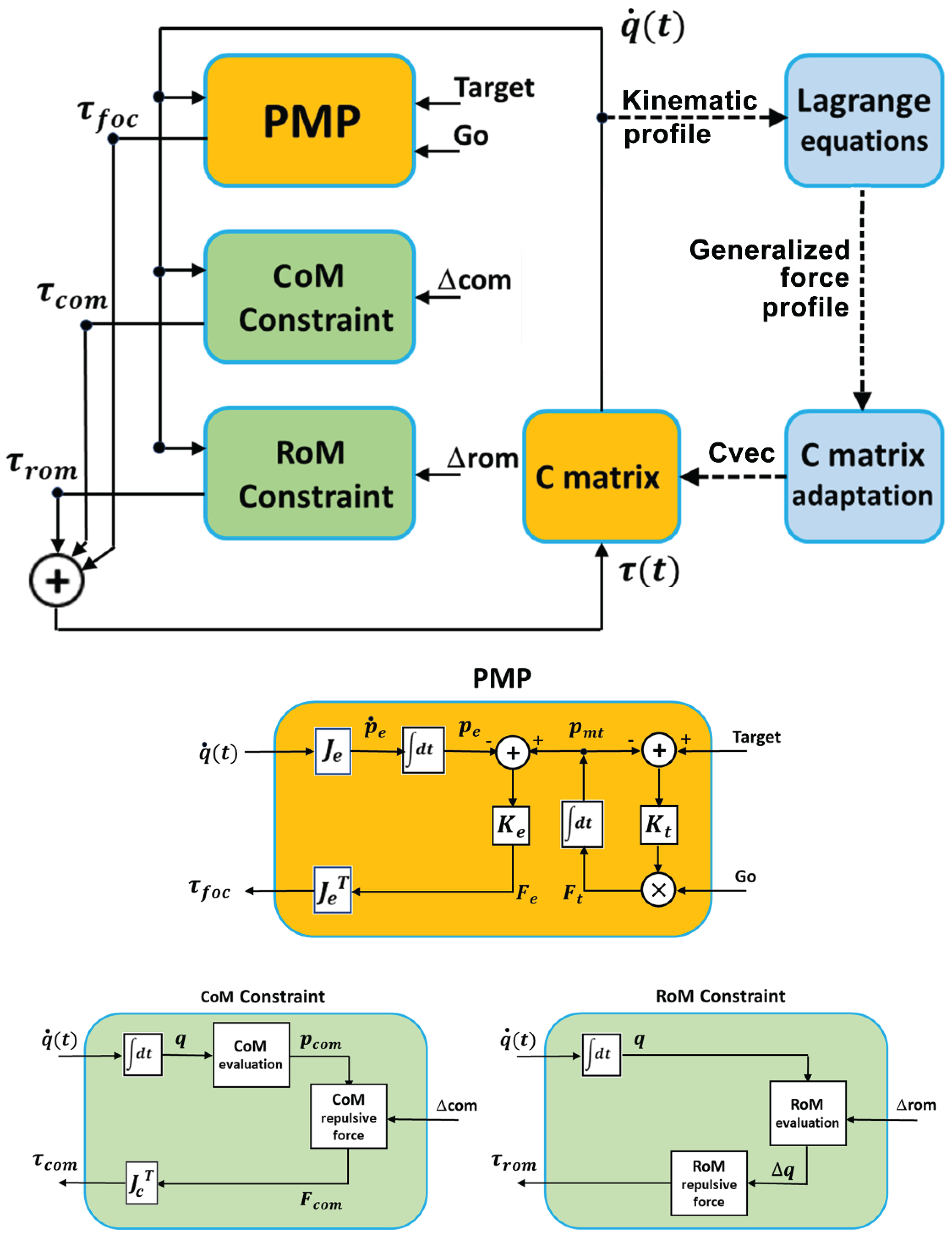
Figure 2.
Geometric model of the simulated robot.
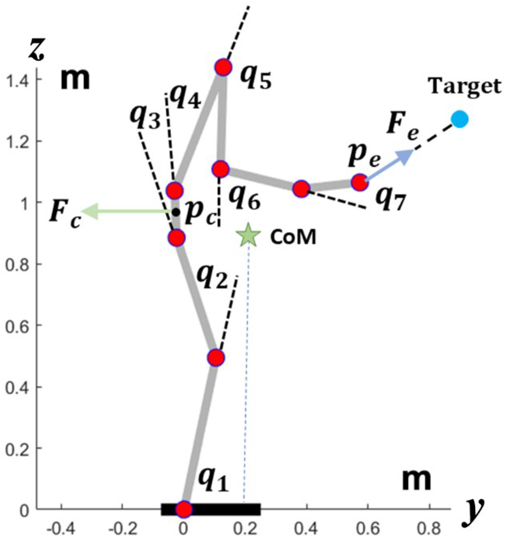
Figure 3.
Panels A1 and A2 represent the initial and final posture of an action with the same duration of 1 s, the same initial posture, the same final target and zero load but different . The two vectors are plotted in panel B3: red markers correspond to A1 and blue markers to B1. The corresponding torque profiles generated by the Lagrange equations are plotted in panels A2 and B2. Panel C shows the joint rotation patterns related to A1 (blue traces) and to A2 (red traces).
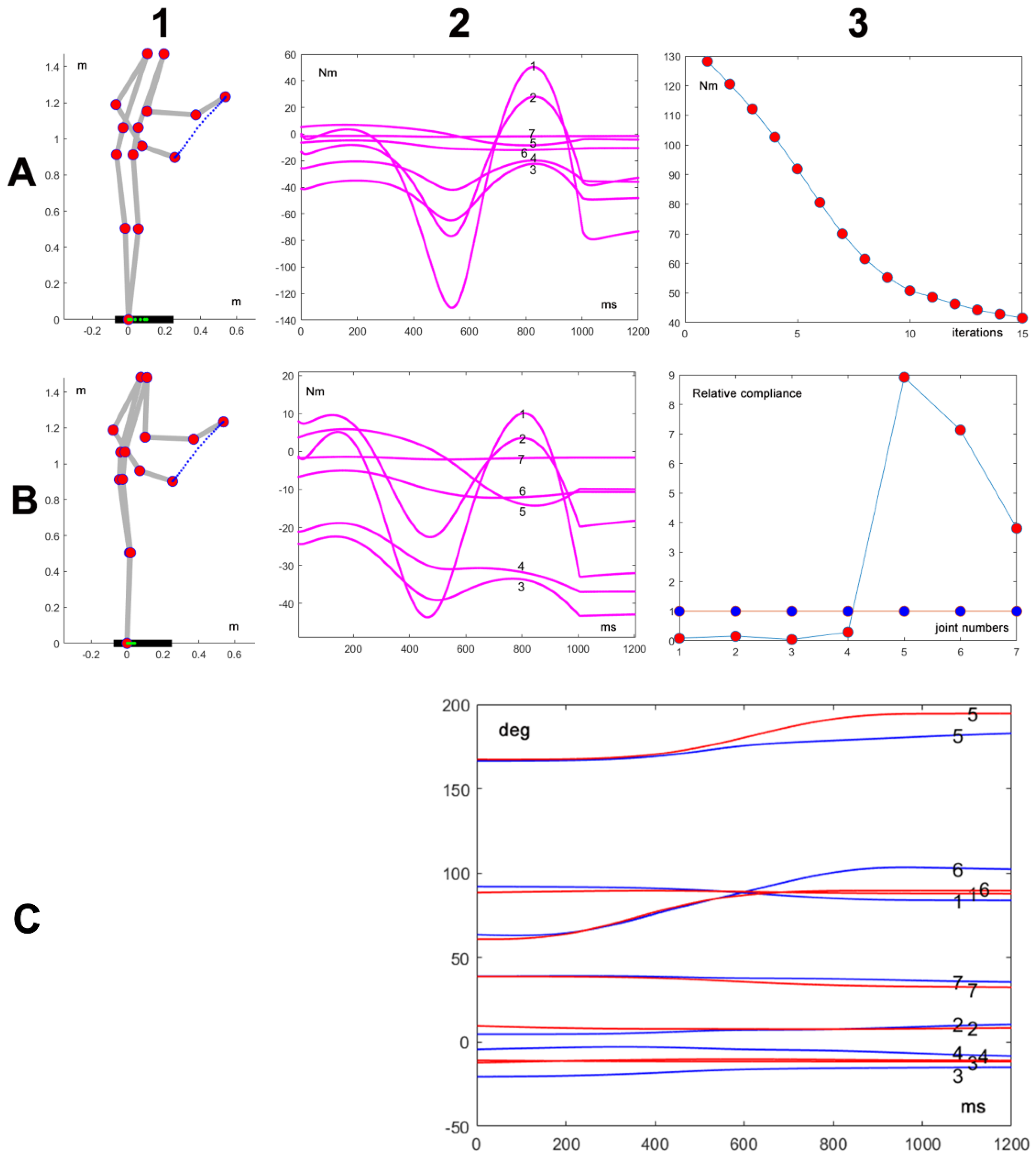
Figure 4.
A, B, C correspond to three simulations with the same initial posture, the same duration of 1s, the same target distance of 0.43m, no load, but different final target. Panels 1 represent the initial and final posture of simulations with the uniform , plotted in panels 4 with blue markers. Panels 2 represent the initial and final posture of simulations with the adapted , plotted in panels 4 with red markers.The corresponding torque profiles generated by the Lagrange equations are plotted in panels A2 and B2. Panel C shows the joint rotation patterns related to A1 (blue traces) and to A2 (red traces).
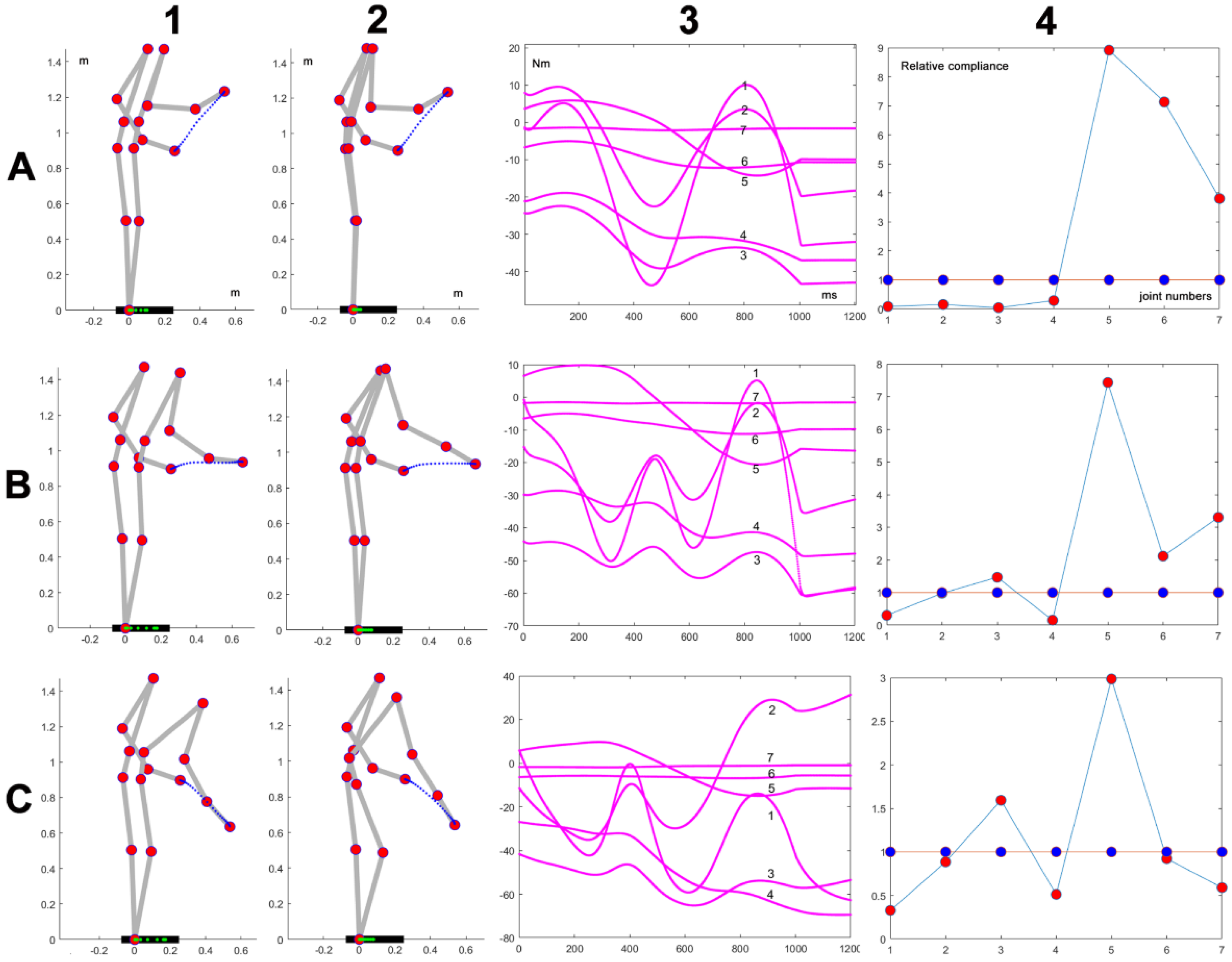
Figure 5.
The three simulations differ for the load: no load (A), 20kg load (B), 40kg load (C). The direction of the movement and the distance of the target is the same (0.43m), as the movement duration (1s). A1, B1, C1 show the initial and final postures with the default configuration; A2, B2, C2 show the postures after C-matrix adaptation; A3, B3, C3 show the corresponding torque vectors after adaptation; A4, B4, C4 show the initial (blue markers) and final (red markers) configurations.
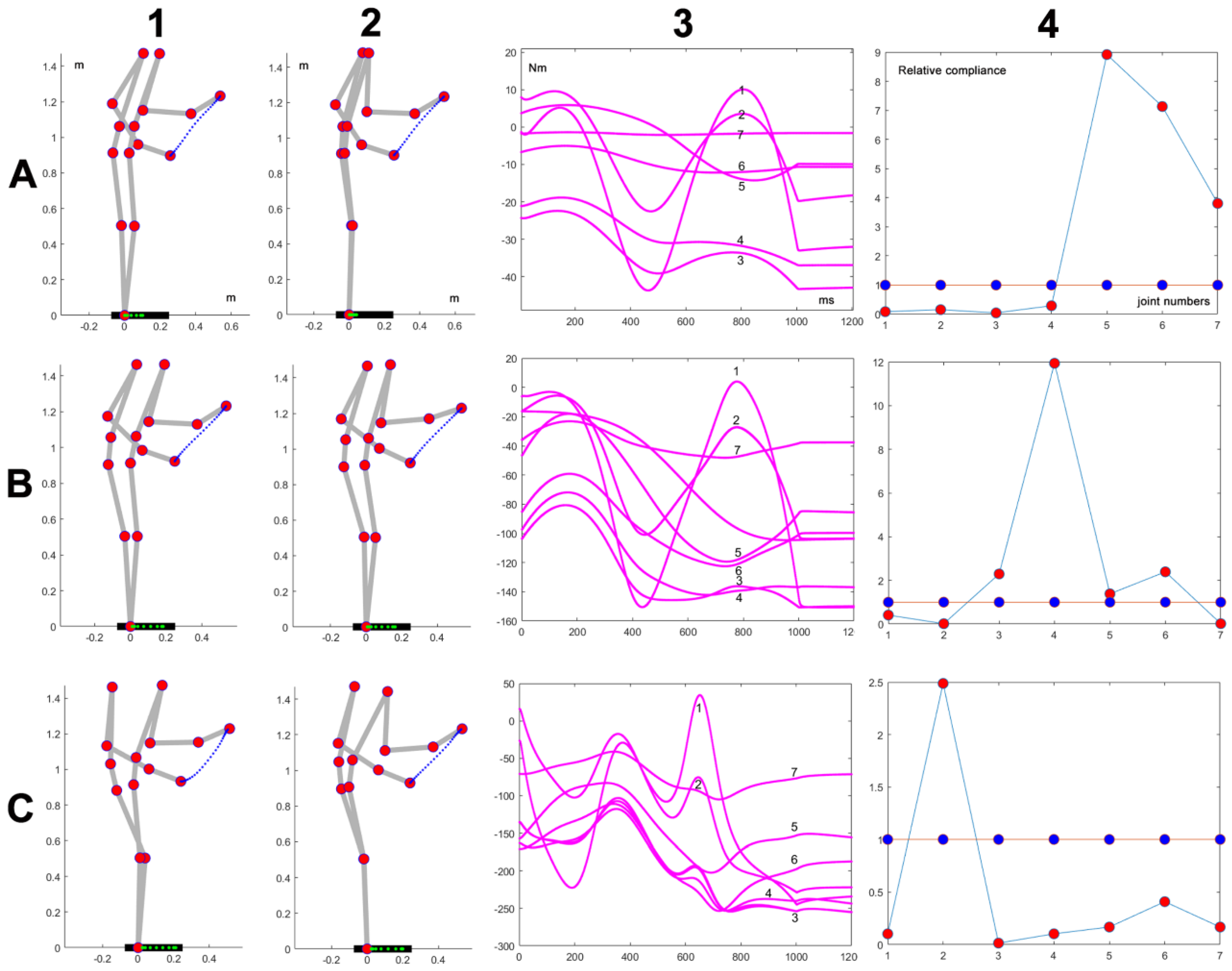
Figure 6.
The three simulations differ for the duration: 1.4s (A), 1s (B), 0.6s (C). The direction of the movements and the distance of the target is the same (0.43m), the load is null. A1, B1, C1 show the initial and final postures with the default configuration; A2, B2, C2 show the postures after C-matrix adaptation; A3, B3, C3 show the corresponding torque vectors after adaptation; A4, B4, C4 show the initial (blue markers) and final (red markers) configurations.
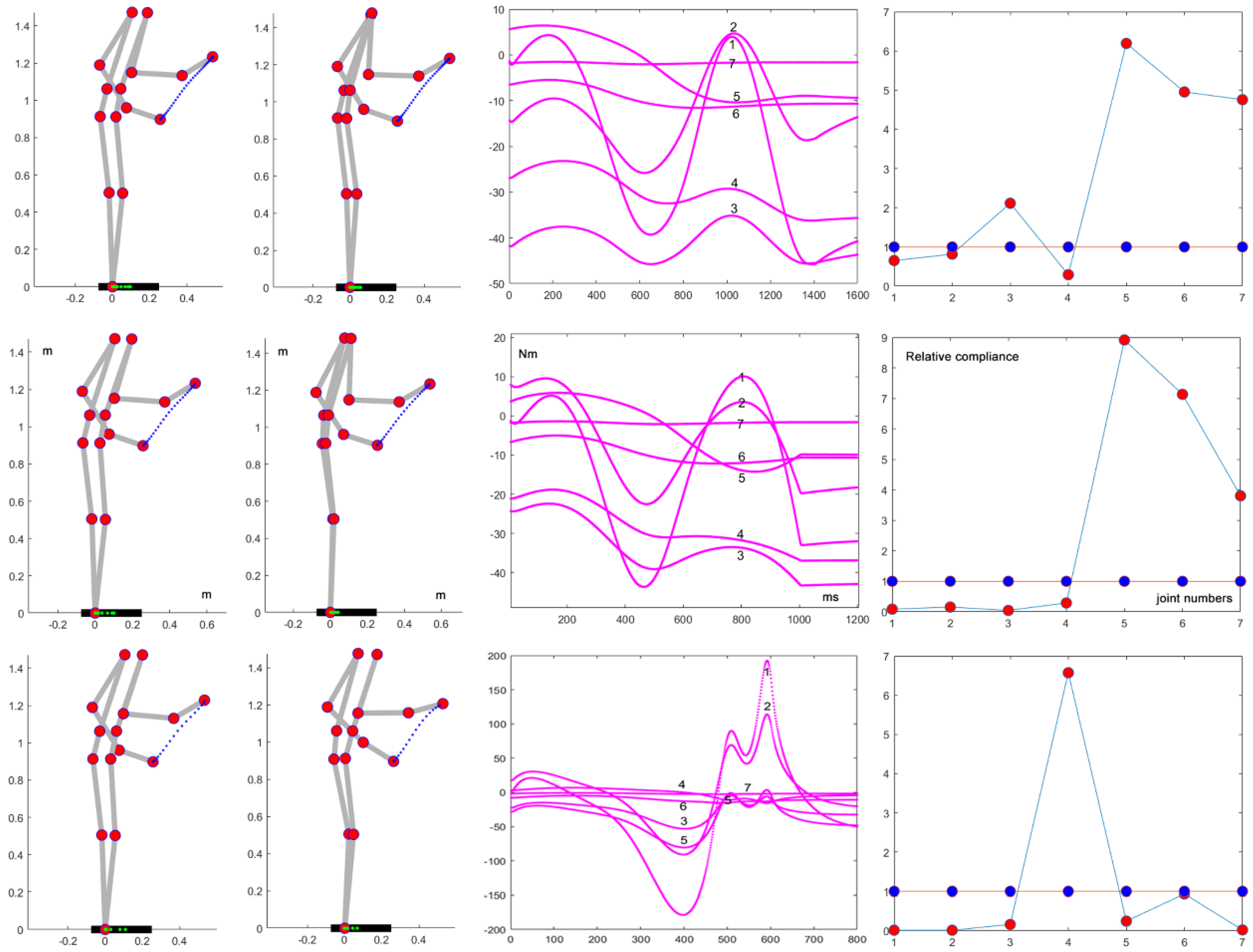

Table 1.
Robot links.
| Segment | 1 | 2 | 3 | 4 | 5 | 6 | 7 | 8 |
| Name | foot | leg | thigh | pelvis | trunk | arm | forearm | hand |
| Length (m) | 0.3 | 0.505 | 0.411 | 0.153 | 0.432 | 0.332 | 0.271 | 0.192 |
| Weight (kg) | 7.6 | 19.6 | 11.8 | 27.3 | 4.2 | 2.8 | 2.2 | |
| Inertia Moment (kg m2) | 0.1615 | 0.2759 | 0.0230 | 0,4236 | 0.0367 | 0.0171 | 0.0061 |
Table 2.
Robot joints.
| Joint | 1 | 2 | 3 | 4 | 5 | 6 | 7 |
| Name | ankle | knee | hip | lumbar | shoulder | elbow | wrist |
| RoM min (deg) | +45 | -10 | -30 | -140 | -210 | 0 | -15 |
| RoM max (deg) | +100 | +120 | +45 | +15 | +10 | +120 | +45 |
Disclaimer/Publisher’s Note: The statements, opinions and data contained in all publications are solely those of the individual author(s) and contributor(s) and not of MDPI and/or the editor(s). MDPI and/or the editor(s) disclaim responsibility for any injury to people or property resulting from any ideas, methods, instructions or products referred to in the content. |
© 2025 by the authors. Licensee MDPI, Basel, Switzerland. This article is an open access article distributed under the terms and conditions of the Creative Commons Attribution (CC BY) license (http://creativecommons.org/licenses/by/4.0/).
Copyright: This open access article is published under a Creative Commons CC BY 4.0 license, which permit the free download, distribution, and reuse, provided that the author and preprint are cited in any reuse.


