

Submitted:
05 June 2025
Posted:
11 June 2025
You are already at the latest version
Abstract
Manufacturing industries are undergoing a significant transformation towards Smart Manufacturing (SM) to cater to the ever-evolving demands of customized products. A major obstacle in this transition is the integration of Computer-Aided Process Planning (CAPP) with Scheduling. This integration poses challenges because of conflicting objectives that must be balanced, resulting in the Integrated Process Planning and Scheduling problem. In response to these challenges, our research introduces a novel hybridized machine learning-optimization approach designed to assign and sequence setups in Dynamic Flexible Job Shop environments via dispatching rule mining, accounting for real-time disruptions such as machine breakdowns. This approach seeks to bridge the gap between CAPP and scheduling by treating setups as dispatching units, ultimately minimizing makespan and bolstering manufacturing flexibility. The problem is modeled as a Dynamic Flexible Job Shop problem, and it is tackled through a comprehensive methodology that combines mathematical programming, heuristic techniques, and the creation of a robust dataset for data mining, which captures attributes reflecting priority relationships among setups. Empirical results validate the effectiveness of our methodology, demonstrating that the mining model surpasses classical dispatching rules. Furthermore, our model exhibits robust generalization capabilities in the context of SM, paving the way for more efficient and adaptive production.
Keywords:
process planning
; dynamic scheduling
; supervised classification learning
; smart manufacturing
; optimization
1. Introduction
Over the last three decades, the manufacturing industry has significantly transformed from traditional manufacturing processes to the Smart Manufacturing (SM) era, driven by the increasing demand for highly customized products. This shift has posed extraordinary challenges for production planning and scheduling, necessitating real-time and flexible approaches to meet these customization requirements. In response, manufacturing systems must autonomously adapt their process plans and production schedules to dynamically changing manufacturing environments.
Process Planning (PP) is critical in linking design and manufacturing, involving decisions related to raw materials, processes, machines, and sequencing operations. Traditional PP largely depends on the knowledge and experience of human experts, potentially leading to inefficient decision-making and non-optimal solutions (Besharati-Foumani, Lohtander, and Varis 2019). This approach also suffers from being nongeneralizable and cannot fulfill mass customization requirements, which requires manufacturing flexibility (Trstenjak and Cosic 2017). Due to the capability of computers to aid planning activities with increased speed and accuracy, the Computer-Aided Process Planning (CAPP) method has been gaining popularity among researchers (Nikolov et al. 2024; Al-wswasi, Ivanov, and Makatsoris 2018). Wu (W. Wu et al. 2020) defined CAPP as a combination of tasks involving translating a part's geometric model into machining features, determining suitable machining resources and operations, and selecting the most cost-effective setup plan and operation sequence considering design and manufacturing constraints. Most CAPP systems use either the variant approach (retrieval of the existing plan and modification) or the generative approach (developing a plan based on part geometry) to generate the process plan (W. J. Zhang and Xie 2007). Despite the efforts, few CAPP systems can significantly improve manufacturing because of the highly complex and dynamic aspects (Al-wswasi, Ivanov, and Makatsoris 2018).
Scheduling allocates manufacturing jobs to manufacturing resources over a specific time interval. The scheduling function depends on the job arrival pattern, operation precedence relation, and the number of available resources and determines the most suitable time to execute an operation on a machine tool. In summary, scheduling is an optimization problem where the objective is to manufacture final products in the shortest possible time considering resource capacity limitations (Shen, Wang, and Hao 2006). PP and scheduling are two separate manufacturing activities; however, both functions are closely related. PP can also be considered a manufacturing resource management function; PP and scheduling objectives are incompatible and usually in conflict. Where scheduling usually considers manufacturing resources with time-based objectives, PP mainly focuses on minimizing manufacturing cost and product quality objectives. Traditionally PP and Scheduling are done sequentially; scheduling is done after PP. This approach has some significant drawbacks. According to Li et al. (Xinyu Li and Gao 2020), the process planner creates a process plan for individual jobs within the sequential approach. The capacity limitation of resources and uncertain events, such as delays, urgent orders, and machine breakdowns, are not considered in this stage. During the scheduling phase, this fixed process plan often becomes infeasible due to the dynamic changes in the production floor. Thus, it is crucial to study the overlap between the PP and scheduling objectives to handle this kind of disruption of the production floor.
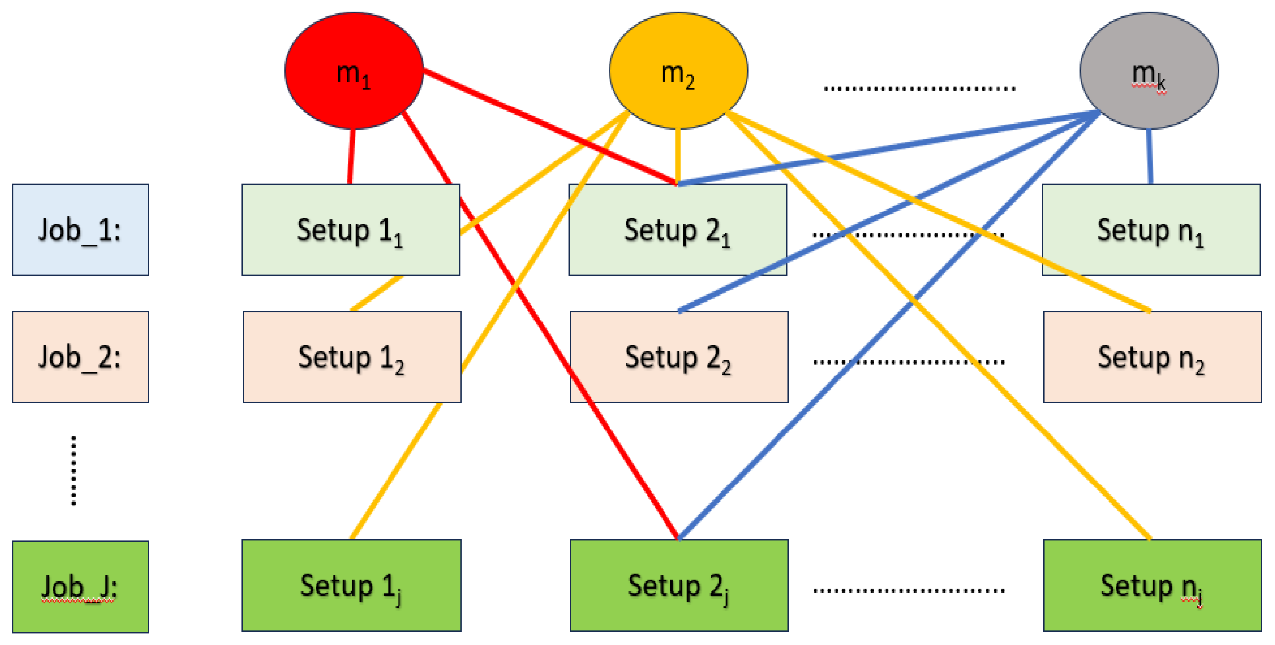
The integrated CAPP and scheduling problem in this research involves completing jobs on m machines, each comprising multiple setups (). This problem is modeled as a Flexible Job Shop Scheduling Problem (FJSP). The goal is to assign setups to machines and sequence them to minimize makespan while following the logical sequence of setups within each job.
Figure 1.
Schematic view of the problem.
This research aims to create an ML-Optimization model to tackle the integrated CAPP and Scheduling problem. The research has several key contributions:
- to conduct an in-depth analysis of existing literature related to Integrated Process Planning and Scheduling (IPPS) approaches, providing a comprehensive understanding of the field,
- to develop an initial schedule that solves the machine assignment and sequencing problems, forming the basis for subsequent analyses and optimizations,
- to formulate a mixed-integer linear programming (MILP) model specifically designed for sequencing setups efficiently,
- to create a machine learning model tailored for extracting dispatching rules, utilizing data-driven insights to enhance scheduling efficiency,
- to apply the developed model in real-world scenarios, validating its practicality and assessing its effectiveness in solving the integrated CAPP and Scheduling problem.
- and, to showcase the model's adaptability by demonstrating its ability to handle dynamic manufacturing environments, including rescheduling in response to unpredictable events.
This introduction has provided an overview of the research problem statement, objectives, and research questions. Subsequent sections of the manuscript will delve into literature review in section 2, research methodology in section 3, and findings in section 4, concluding with recommendations for future studies in section 5.
2. Literature Review
This section presents a critical review of the relevant literature, followed by a discussion of the concluded gaps.
2.1. Review of IPPS
The IPPS problem is one of the most intricate problems for manufacturing systems (Haro et al. 2024). In most research papers addressing the IPPS problem, it is typically dissected into three subproblems: (i) the selection of process plans, (ii) the allocation of machines, and (iii) scheduling (Barzanji, Naderi, and Begen 2020). The conventional approach to addressing this problem involves first, choosing the process plan, followed by the subsequent allocation and scheduling of operations (Barzanji, Naderi, and Begen 2020; X. Wu and Li 2021).
All of these approaches consider operations as the dispatching unit. Operation sequencing is a common problem for both process planning and scheduling functions. For PP, operations of a job are sequenced with objectives such as minimizing machining costs (Priyabrata Mohapatra, Nanda, and Maji 2015). In the case of scheduling, the operations are sequenced to complete the jobs in the shortest possible time (Alemão, Rocha, and Barata 2021; Parente et al. 2020; Wenzelburger and Allgöwer 2021; Liu et al. 2019). This creates conflict between the objective of PP and scheduling. Process planning might involve trade-offs between cost and other factors like quality, production time, or resource utilization. For example, using a slower machine that consumes less energy and produces might be cost-effective but increase production time. On the contrary, scheduling decisions often prioritize time over cost. This can lead to situations where machines are frequently set up or reconfigured for different jobs, which might not be the fastest manufacturing approach
Now, setup planning can play a crucial role in bridging the gap in this conflict. (Haddadzade, Razfar, and Zarandi 2016). Setup planning is a pivotal task within CAPP that guides workpiece setup, influencing manufacturability, production efficiency, costs, and the integration of CAD/CAPP/CAM/CNC, thus advancing intelligent manufacturing (Y. Zhang et al., 2022). It is divided into three sub-tasks: setup generation by grouping manufacturing operations, operation sequencing within setup, and setup sequencing (Ming et al. 2000; Joshi et al., 2008). Many works dedicated to the IPPS problem acknowledged the importance of setup planning for the integration of CAPP and the Scheduling function. For instance, Mohapatra et al. (2015) proposed adaptive setup grouping strategies for minimization of cost and makespan and maximization of machine utilization for alternative machines (3-axis, 4-axis, 5-axis, etc.) for a single part. They have focused on grouping operations for a workpiece and assigning each setup to suitable machines, following a cross-machine setup approach. However, they neglected the importance of addressing the true integration of the process planning and scheduling problem, which should involve the consideration of n parts to be processed on m machines. To solve the issue, Haddadzade et al. (Haddadzade, Razfar, and Zarandi 2016) proposed a cross-machine setup planning approach for multiple parts and grouped operations simultaneously targeting various objectives. Although, this research does not consider the routing and sequencing task of the problem.
Furthermore, there is currently an increase in the number of Adaptive Setup Planning (ASP) studies focusing on generating machine-specific setups upon request from dynamic schedule (Cai, Wang, and Feng 2009). Adopting such an ASP approach has the advantages of adapting to unforeseen events, such as changes in machine availability, fixtures, and tools, and significantly decreasing the time required for re-planning and rescheduling. Thus, it is necessary to consider setups as the dispatching unit for scheduling instead of operations. Cai et al. (2009) reinforced the use of setups as the dispatching and scheduling unit of machining.
From the literature review (Table 1), it becomes apparent that most previous research has primarily concentrated on addressing the process plan selection and routing problem under static conditions. While some studies have demonstrated the potential to adapt setup plans to changing shop floor conditions, they have not effectively tackled the sequencing problem within dynamic scenarios.
However, static scheduling becomes outdated when unforeseen events occur on the shop floor due to unrealistic assumptions considered during their creation. Liu et al. (2021) point out in their review that deterministic scheduling assumptions, like known and fixed processing times and the absence of machine failures, render these static schedules impractical in real-world situations. As Industry 4.0 continues to evolve, the production system is gaining enhanced flexibility; this progress comes hand in hand with added intricacies in production scheduling. Manufacturing systems inevitably face unpredictable disruptions, causing changes in planned activities due to factors such as resource availability shifts, order arrivals or cancellations, and longer processing times. Consequently, there arises a necessity for scheduling mechanisms to swiftly adapt to these potential disruptions and efficiently re-optimize the operational sequences in real-time (Ferreira, Figueira, and Amorim 2022).
Therefore, this research takes a novel approach by treating the setups for each job or workpiece as the dispatching and scheduling unit. The objective is to encompass the problem of PP within the dynamic scheduling framework. This innovative approach allows for the development of a one-shot solution method for the integrated CAPP and scheduling problem. Furthermore, it facilitates the reconfigurability of the process plan, as highlighted by Azab and ElMaraghy in 2007 (Azab and ElMaraghy 2007).
2.2. Dynamic Scheduling for Smart Manufacturing
The challenge of managing schedules while accounting for real-time events (i.e., disruptions) is referred to as dynamic scheduling. The purpose of this scheduling type is to offer a partial or complete reconfiguration of the production schedule to lessen the effect of disruptions (Ouahabi et al. 2024). Research has developed into dynamic scheduling to address real-time disruptions, treating it as a series of static scheduling problems that require periodic revision or updates triggered by real-time events. The methodology of Dynamic scheduling can be grouped into proactive-reactive and predictive-reactive approaches (Ferreira, Figueira, and Amorim 2022; Priore et al. 2014). The aim of the predictive-reactive approach is to develop a preliminary schedule that seeks to mitigate the effects of uncertain events on overall system performance (Ouelhadj and Petrovic 2009). To adjust the preliminary schedule or reschedule, we need to answer two questions: when and how to react to uncertain events. Three policies, periodic, event-driven, and hybrid rescheduling, are suggested in the literature to address the questions as to when to reschedule and how to reschedule. Schedule repair and complete rescheduling are also tackled in the literature (Priore et al. 2014).
Existing scheduling methodologies can be grouped into three categories: exact approaches, meta-heuristic algorithms, and heuristic approaches (Priore et al., 2014; L. Zhang et al., 2022). Exact approaches based on mathematical modeling have been used to ensure better performance than other heuristic methods in terms of finding optimal solutions. Approaches such as mixed-integer linear programming, branch and bound can find the optimal solutions for small or mid-size scheduling problems (Jun, Lee, and Chun 2019). However, they are computationally inefficient for large-scale problems because they cannot solve the problems in polynomial times (Jun, Lee, and Chun 2019). Metaheuristics [e.g., simulated annealing (SA), tabu search, genetic algorithms (GAs)] are widely applied to solve large scheduling problems (Priore et al. 2014). For instance, Chen et al. (2024) proposed a Q-Learning-based NSGA-II algorithm for a dynamic flexible job shop with transportation resources. However, Meta-heuristic algorithms are time-consuming, and their performance can even vary dramatically among different problems, especially for solving dynamic or online scheduling problems. Shahzad and Mebarki stated in their work that, although metaheuristics have an advantage over heuristics, such as dispatching rules in terms of solution quality and robustness, these are usually more difficult to implement and tune and are computationally too complex to be applied in a real-time system (Shahzad and Mebarki, 2012). Ouelhadj and Petrovic (2009) have reported in their study that hardly any research has addressed the use of metaheuristics in dynamic scheduling.
Currently, in literature, a common and popular way of dynamically scheduling jobs is by implementing dispatching rules. Dispatching rules are efficient, simple, and capable of instantly solving scheduling problems by assigning a priority for every job in the waiting queue and are frequently used in practice due to their ease of implementation and quick computation time (Renke, Piplani, and Toro 2021; Jun and Lee 2021; Kianpour et al. 2021; S. Zhang et al. 2021). However, as dispatching rules are traditionally derived by empirical or analytical studies, the performance of these rules depends on the state the system is in at each moment (Priore et al. 2014). To resolve this limitation and boost their effectiveness/performance, machine learning algorithms arise as a promising solution (Priore et al. 2014; Ferreira, Figueira, and Amorim 2022; Taghipour et al. 2024; Wu et al. 2024 ). Among the two approaches of dynamic scheduling, a knowledge-based system is capable of extracting implicit knowledge from earlier system simulations to determine the best dispatching rule for each possible system state.
The main algorithm types in the field of dispatching rule development are case-based reasoning (CBR), neural networks, inductive learning, and reinforcement learning. The Inductive Learning Algorithm (ILA) is an iterative and inductive machine learning approach employed to generate a set of classification rules, typically presented in the "IF-THEN" format, based on a given set of examples. This algorithm progressively refines its rule set through successive iterations, appending newly generated rules to the existing set. Shahzad et al. (Shahzad and Mebarki 2012) proposed a hybrid simulation-optimization-data mining approach to generate JSP solutions by tabu search and identified the dominant relationship between competing jobs with predefined attributes. A decision tree is subsequently employed to dispatch jobs in real-time efficiently. Zhao et al. (2022) constructed a data mining dynamic scheduling model to assign Dispatching Rules (DRs) from a DR library to different scheduling subproblems in real-time. Metan et al. (2010) have also developed a decision tree learning model to select dispatch jobs in real-time. Habib Zahmani and Atmani (2021) have developed a GA-datamining approach to automatically assign different dispatching rules to machines based on the jobs in the queues. This work tried to address the dominance or priority of different jobs. Olafsson and Li (2010) are one of the pioneers in developing a data mining-based approach to discovering new dispatching rules for operation sequencing of multiple jobs. They used a decision tree to discover key scheduling decisions from production data. Liping et al. (2022) have investigated new dispatching rules for operation sequencing development through the optimization of scheduling along with the data transformation and mining through a hybrid GA-random forest algorithm. Jun et al. (2019) have also taken a similar approach to developing operation assignment and sequencing rules using random forests. From this, it becomes evident that developing a dispatching rule mining system for dynamic setup sequencing can be beneficial for addressing the current gap in the integrated CAPP and Scheduling problem.
Based on the literature review presented, this study adopts a predictive-reactive approach to effectively sequence setups on the shop floor to address the gap in process planning and scheduling objectives. By integrating machine learning and optimization within a unified framework, the schedule can be dynamically adjusted in response to these disruptions, all while ensuring that the fundamental objectives of the Integrated CAPP and Scheduling problem remain unviolated.
3. Methodology
We introduce a novel approach that combines machine learning (data mining) and optimization techniques for addressing the integrated CAPP and Scheduling problem. The primary objective of this approach is to create a set of rules for guiding dispatching decisions to sequence setups within a flexible job shop scheduling environment. Thus, initial nominal solutions for small problem instances are generated as sources of learning rules for scheduling. Once the solutions have been obtained, they are transformed into learning data by constructing new attributes. In this research, the term ‘attributes’ refers to the set of all data related to the scheduling decisions. The proposed approach first assigns setups to available machines on the shop floor. Secondly, setups are sequenced on an assigned machine by learning the best dispatching rule through an ML-Optimization model. Finally, considering an event of a random machine breakdown, the initial schedule is adjusted by re-assigning disrupted setups on the new available machine and sequenced utilizing the mined dispatching rule.
The methodology is described as follows:
- Initially, a simulation module generates a series of problem instances relevant to real-world scheduling systems. Alternatively, historical data from the manufacturing system can be used in place of this. These problem instances are then stored in an instance database.
- Subsequently, the optimization module generates solutions for a subset of these instances, from which the initial training dataset is created. These solutions represent a collection of well-informed scheduling decisions that could potentially benefit the manufacturing system. These scheduling decisions form valuable scheduling knowledge, stored in a scheduling database, and utilized by a learning process to construct a decision tree. This decision tree is then used for generating the dispatching rule of the setups. Notably, it is a dynamic sequencing model which can be updated with the change in resources.
- Figure 2 illustrates the dispatching rule mining approach framework for sequencing the setups. Later, the generated rule can also be used to sequence disrupted setups as needed dynamically.
3.1. Solving the FJSP
An FJSP instance can be divided into two sub-problems: a routing problem and a sequencing problem. The routing sub-problem involves assigning each operation to a suitable machine. In contrast, the scheduling sub-problem focuses on determining the order in which operations should be performed while considering precedence constraints. The sequencing problem is for sequencing assigned operations to machines and is equivalent to the classical job shop scheduling problem. These two sub-problems have been shown to be NP-hard (Jun, Lee, and Chun 2019).
The Flexible Job Shop Problem (FJSP) can be approached using two main strategies: concurrent approaches and hierarchical approaches. Hierarchical approaches provide a structured method by independently handling assignments and sequencing decisions, thus reducing the problem's complexity.
A hierarchical methodology is employed to address the research problem in this research study. Specifically, a rule-based algorithm is adopted to tackle the routing problem, thereby transforming the initial problem into a form that can be effectively analyzed and compared with a classical job shop sequencing problem.
3.1.1. Solving the Routing Sub-Problem / Machine Assignment
The routing sub-problem is a crucial aspect of production scheduling and involves the assignment of each operation or task to a suitable machine or workstation. This is a fundamental step in optimizing the production process, as it determines the sequence in which tasks are executed and the allocation of resources.
Solving the routing sub-problem aims to minimize production costs, maximize efficiency and utilization, reduce makespan, or achieve other specific objectives depending on the manufacturing environment and requirements. Various algorithms and techniques, such as mathematical optimization, heuristics, and simulation, can be used to address the routing sub-problem and find an optimal or near-optimal assignment of operations to machines.
In this study, we have employed the approach by localization (AL), summarized in Table 2, which enables us to address the resource allocation challenge and construct an ideal assignment model (Pezzella, Morganti, and Ciaschetti 2008; Vital-Soto, Azab, and Baki 2020). This method considers both the time it takes to complete tasks and the load on each machine, which is the total processing time of the operations assigned to it. The process involves identifying, for each operation, the machine with the shortest processing time, locking in that assignment and subsequently adding this time to all the following entries in the same column (updating the machine's workload), as shown in Table 3, where bold values correspond to workload updates.
3.1.2. Solving the Sequencing Sub-Problem/Job Shop Scheduling (JSP)
Once the assignments are settled, the problem becomes akin to a classical JSP problem. We just need to determine the sequence of the setups on the machines. The sequencing is feasible if it respects the natural precedence relationship among the setups of the same job, i.e., setup Si,j cannot be processed before setup Si,j+1. In this study, the sequencing of the initial assignments is obtained by solving the following Mixed Integer Linear Programming (MILP) model, which is formulated as follows:
The problem considers n jobs that must be processed in m machines. Each job consists of a total of nj setups. Each setup Sij must be assigned to a machine k and find the sequence of the job j. The setup planning solution includes and sets the precedence between the setups of a job. The objective is to minimize the maximum makepan.
The following assumptions are proposed for the FJSP:
- (1)
- All the jobs and machines are available at time zero.
- (2)
- Each machine can perform at most one operation at any time.
- (3)
- Transportation time is not considered.
- (4)
- procession time includes setup time.
- (5)
- Job preemption is not allowed.
- (6)
- The setup numbers are indicative of their natural logical sequence within a job.
The notations used in this paper are defined as follows:
Index:
J: Number of jobs
j: The index of jobs of {1,2,..,J}
m: Number of machines
k: The index of machine {1,2,..,m}
nj: Number of setup in a job j
i: The index of setup {1,2,..,nj
Parameter:
: Processing Time of setup i of job j on machine k
M: a very large positive number
=
Decision variables:
: start time of the setup i of job j on machine k
=
: Makespan
MILP Model:
s.t.,
The objective function is defined by Eq. (1), which minimizes the makespan. Constraint set (Eq. (2)) defines the start time for each setup on the assigned machine. The disjunctive sets (Eqs. (3) and (4)) are feasibility constraints that ensure that only one setup of a job processed on a machine at a time and precedence relationship is followed. The disjunctive constraint sets (Eqs. (5) and (6)) avoid the overlapping of setup on same machines of different job at a time. Constraint sets (Eq. (7)) define the maximum make span. Constraint set (Eq. (8)) ensures that the starting time and make span should be either positive or zero. Constraint sets (Eqs. (9) define the types of variables.
The goal of the experiment is to solve the problem instance to generate quality solutions (makespan). OR-Tools2 (ORT), an open-source solver developed by Google(Da Col and Teppan 2019b). In this research, we employed Google’s OR-Tools to find the sequence of the initial assignment. Concerning the solvers’ version, we use version 9.6 for OR-Tools. We have decided to use the CP-SAT solver because CP-SAT has proven to be better on average, as reported in the literature, is fairly easy to implement, and is compatible with other necessary Python libraries and packages (Da Col and Teppan 2019b; 2019a). The experiment is conducted on a system equipped with a 3 GHz Intel Core i7 4-Core (11th Gen), 16GB of DDR4 RAM, and a 256GB M2 SSD.
3.2. Construction of Data Mining Dataset from Initial Solution
Creating an appropriate training dataset is a pivotal aspect of the entire rule-mining procedure. When viewed from the perspective of setup sequencing, the primary objective is to identify the preferred order in which setups should be prioritized for dispatching among a collection of schedulable setups, regardless of whether they belong to the same or different jobs and are intended for the same machine at a specific moment. By extracting this knowledge from the training dataset, we can determine the sequence for dispatching the next setup at any given time. Subsequently, this knowledge can be used to generate dispatching lists for any combination of jobs and machines, provided that the assignment or routing for each setup is known.
3.2.1. Attributes Selection
Attribute selection is the task of identifying the most appropriate set of attributes for a classifier, with the aim of reducing the number of attributes while maximizing the separation between classes (Shahzad and Mebarki 2012). This process is crucial for the effectiveness of subsequent model induction since it helps eliminate redundant and irrelevant attributes. However, it is also important to note that the attributes recorded as part of the available data may not always be the most relevant or useful for the data mining process, making the creation of new attributes a necessary consideration.
Priority relationship can be formed between the jobs while the sequencing based on their processing time, due date etc. (Shahzad and Mebarki 2012; Xiaonan Li and Olafsson 2005; Olafsson and Li 2010). This priority relationship can be reduced by only considering two setups on the same machine, among schedulable jobs, at any given instance for comparison. However, proper attribute selection is essential for capturing this relationship.
Furthermore, both the selection of raw attributes from production data and creation of new attributes are closely tied to the objectives of the scheduling problem. Objectives related to making span require different attributes to be considered compared to objectives related to flow time or tardiness. For example, attributes related to processing time, precedence relationship and associated statistics are more suitable for makespan or completion time-based objectives. Similarly, attributes related to deadlines and associated statistics are more suitable for tardiness-based objectives.
Additionally, the attributes that are recorded as part of the raw production data may not be the attributes that are the most useful for the data mining itself. Thus, new attributes creation must be considered. (Shahzad and Mebarki 2012; Xiaonan Li and Olafsson 2005; Olafsson and Li 2010). Combining raw attributes through arithmetic operations can lead to the creation of new valuable attributes, as pointed out by Olafsson and Li (2010). However, it is important to avoid having a large set of attributes, as they are often not independent of each other, which can make the process computationally impractical (L. Zhang et al. 2022).
This study considers 11 attributes belonging to two types, raw and constructed. The four raw attributes based on are the setup processing time (pijk) and the due date of the job (dj). These are considered directly from production data. Constructed attributes can further be divided into two types. Composite attributes and categorical attributes. 2 composite attributes are constructed with basic arithmetic operations following the methodology proposed by Li and Olafsson, (Xiaonan Li and Olafsson 2005; Olafsson and Li 2010). The categorical attributes represent binary variables used to indicate a direct comparison between two setups, A and B. When the raw attribute value of A exceeds that of B, the categorical value is set to 1. Conversely, when the raw attribute value of A is less than that of B, the categorical value is set to -1. For all other situations, the categorical value is set to 0. In this research, 5 categorical attributes are also constructed to capture the priority, delay, and precedence relationship among setups. Details of the attributes are shown in Table 4.
3.2.2. Creation of Training Dataset
The goal of this step is to convert the initial nominal scheduling solution into training data. From the previous steps, nominal solutions for each problem instance are saved as a flat data file. The columns represent separate data attributes, and each row of the file represents the schedule of a setup. Then the training dataset for sequencing setups is generated by following 2 steps, as shown in Figure 3.
- First, the first setup in the schedule list is selected and all setups that can be processed at the start time are taken. Subsequently all possible combinations of setup pairs are selected. Thus, for a problem instance with j job each having i setups, there will be 2 x possible setup pair.
- Then, rows for all possible pairs of setups are appended to a dataset with their attributes.
3.3. Development of Dispatching Rule Mining Model
The setup sequencing rule or dispatching rule is mined using the following supervised learning methodology. The implementation details are described in the following sections.
3.3.1. Preprocessing of the Data
Preprocessing the data, including feature selection and data cleaning, such as handling missing, outliers, inconsistent, skew values, removing duplicates, ensuring data format consistency, correcting typos, errors, dealing with irrelevant or redundant information etc. In the present scenario, case studies have been meticulously crafted through simulation. Nevertheless, it is imperative to emphasize the significance of this step, particularly when dealing with datasets derived from real-world manufacturing systems.
3.3.2. Model Selection
The choice of potential classifiers suitable for the problem depends on the problem's complexity, dataset size, interpretability needs, and available algorithms. For this research, Random Forest, K-Nearest Neighbors (KNN), Support Vector Machine (SVM), Naive Bayes, and Logistic Regression is chosen which represent a mix of ensemble, instance-based, linear, and probabilistic algorithms. These classifiers offer a range of strengths and weaknesses, and they are widely recognized and applied in various classification scenarios. Given the relatively small dataset size and the need to understand the behavior of different algorithm families, these choices provided a comprehensive baseline for assessment.
3.3.3. Parameter Tuning
Identify hyperparameters specific to the chosen models (e.g., learning rate, number of trees, regularization strength) that affect model performance. We investigated the typical variation of parameters for each learning algorithm. This section provides a summary of the parameters employed for each learning algorithm (Caruana and Niculescu-Mizil 2006).
Random Forest (RF): The number of trees in the forest varies between 50 to 500. The number of features to consider when looking for the best split was 1, 2, 4, 6, 8 and 11.
KNN: We used 10 values of k ranging from k = 1 to (number of sample). The standard Euclidean distance was used as distance computation matric.
SVM: The following kernels were used: linear, polynomial degree 3 and radial with kernel varying coefficient (1 / (n_features * X.var()), 1 / n_features, 0.001, 0.01, 0.5, and 1)
Naive Bayes (NB): We employed Gaussian Naive Bayes.
Logistic Regression (LR): Regularized logistic regression is employed. Tolerance was varied by a factor of 10 from 10-5 to 105.
3.3.4. Cross Validation
This study uses stratified K-fold CV on the dataset to perform 5- and 10-fold cross-validation. The dataset is shuffled to have representative folds.
3.3.5. Model Evaluation Metrics
In this research, the best-performing model based on its performance on the cross-validation set is selected and assessed against the test set, which it has never seen before. This gives an estimate of its generalization ability. To evaluate the performance, the approach proposed by Caruana and Niculescu-Mizil (2006) has been adopted. In this evaluation process, we have calculated performance metrics based on seven evaluation parameters: Accuracy (ACC), F-score (FSC), Receiver Operating Characteristic (ROC) score, Precision (APR), Recall (REC), Root Mean Square Error (RMS), and Cross-Entropy (MXE), as well as the execution time (TIME).
3.4. Reconfiguration of Initial Nominal Schedule Under Disruption
This section explains the rescheduling strategy. The rescheduling strategy employs dynamic adjustments to the existing schedule, prioritizing the reassignment of affected jobs to alternative available machines. This ensures production can resume as swiftly as possible following a breakdown event. In this research, we have considered an FJSP with a machine breakdown problem based on the following definitions and assumptions:
Index:
J: Number of jobs
j: The index of jobs of {1,2,..,J}
m: Number of machines
k: The index of machine {1,2,..,m}
nj: Number of setup in a job j
i: The index of setup {1,2,..,nj}
: A subset of machines for setup i
⊆ (m1, m2,.., mk)
Parameter:
: Processing Time of setup i of job j on machine k
=
= Mean time between breakdown of machine k
: Processing Time of setup i of job j on machine k
: Breakdown probability threshold of machine k
Decision variables:
=
: start time of the setup i of job j on machine k
: end time of the setup i of job j on machine k
: Breakdown time of machine k,
Assumptions:
The occurrence of machine failures is modeled as following an exponential distribution
During a production cycle, only one machine will experience breakdown
3.4.1. Machine Breakdown Distribution
According to the assumption of He and Sun (He and Sun 2013), breakdown probability follows the exponential distribution.
Here, Pk = Probability of machine failure, rbk = Estimated repair time, ʎ = 1/Mean time between two successive breakdowns
Following this assumption, this thesis introduces a Monte Carlo simulation-based approach to model the probability of breakdowns occurring over a production cycle. The simulation model is implemented using Python, leveraging the random and matplotlib libraries.
Simulation model for Machine Breakdown:
- Setting the Mean Time Between Breakdowns (lambda): The mean time between breakdowns (lambda) is a key parameter that influences the simulation's behavior. This parameter is user-adjustable, allowing different real-time scenarios and system characteristics to be explored.
- Generating Random Breakdown Times: Using an exponential distribution, the simulation generates random breakdown times for each machine independently. We conduct 1000 simulations for each machine to collect data on breakdown times.
- Calculating Breakdown Probability: We compute each machine's breakdown probabilities at various time points. This allows us to construct cumulative probability curves specific to each machine.
In this research, If the probability function exceeds a specified threshold, the machine will experience a breakdown. Multiple breakdowns are not considered to simplify the problem.
3.4.2. Rescheduling Framework
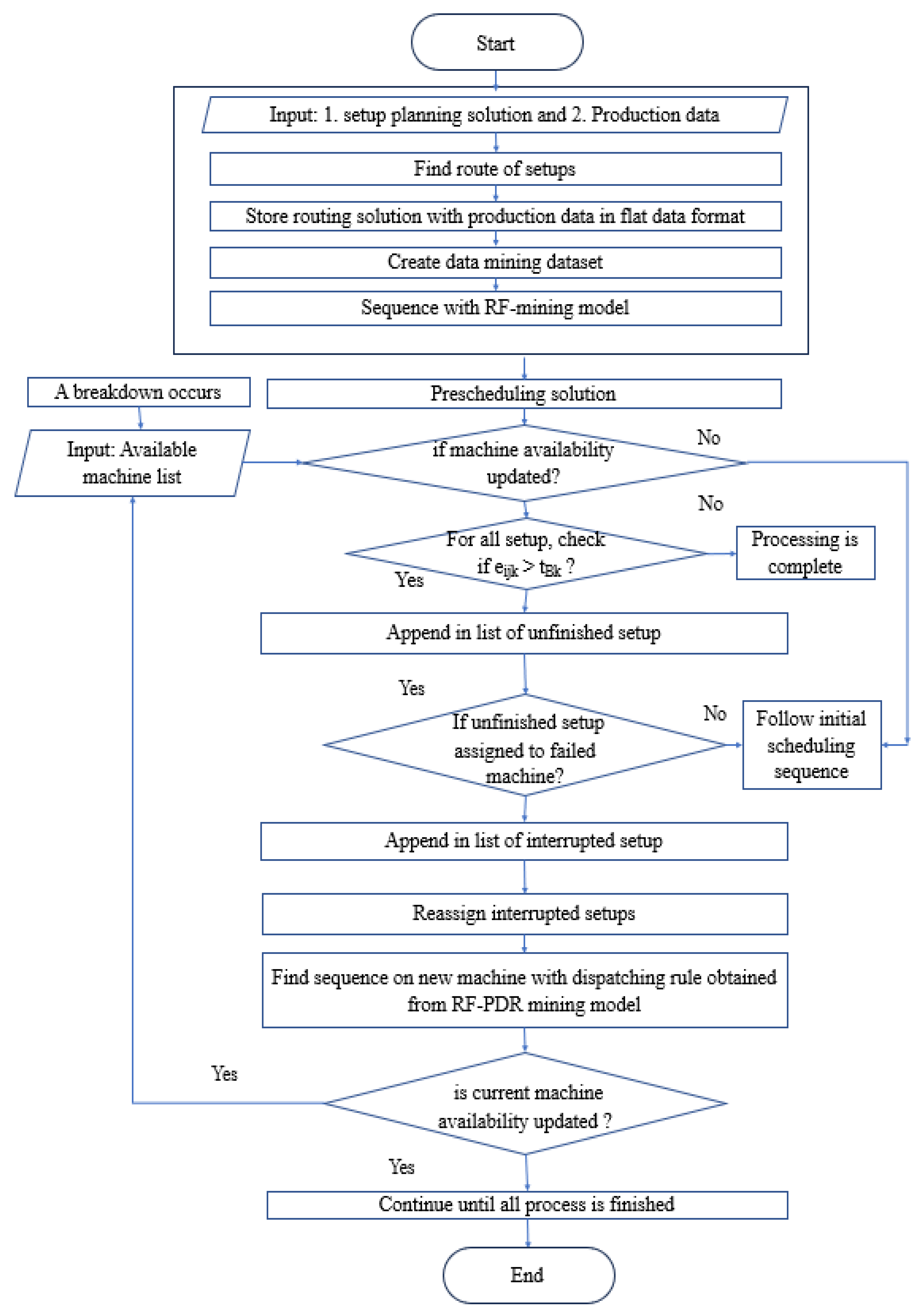
To address rescheduling in response to machine breakdowns, a comprehensive strategy is proposed, which is outlined in the following framework (Figure 4):
Assuming an initial state at t = 0, where the probability of machine breakdown is zero, the prescheduling process is initiated on the job floor, and setups are executed in accordance with the initial nominal scheduling solution. In instances where no machine breakdown occurs, this schedule becomes the realized schedule. As the probability of machine breakdown surpasses a predefined threshold, machine failures are anticipated. Subsequently, the following decision criteria must be evaluated:
- Identification of Interrupted Setups: A critical assessment is conducted for all setups in progress on the broken machine at the time of breakdown. Setups categorized as "interrupted setups" if their scheduled end time exceeds the breakdown time.
- Reassignment of Interrupted Setups: To resume production without delay, these interrupted setups must be reassigned to currently available eligible machines. This reassignment is executed following a localization heuristic approach.
- Sequencing of Interrupted Setups: Once the setups have been reassigned to new machines, their sequence is determined using a dispatching rule derived from the RF-PDR mining model.
- Continuation of the Rescheduling Process: The rescheduling process is iteratively executed until the machine is repaired and brought back into operational condition. Throughout this process, the current availability of resources is continuously considered to ensure optimal scheduling decisions.
This rescheduling framework is designed to effectively address machine breakdowns, minimizing disruption to production processes and optimizing resource utilization systematically and adaptively.
3.4.3. Robust and Stability Measures of Rescheduling
The rescheduling implemented on the job floor is characterized by two crucial attributes: robustness and stability. Developing a rescheduling system that embodies robustness and stability is imperative to mitigate the impact of unforeseen disruptions. In this study, the robustness and stability metrics are adopted from He and Sun’s (2013)and defined as follows:
Here, CmaxR = makespan after rescheduling, Cmaxp = makespan of prescheduling.
The stable measures can be articulated as follows:
Here, n′ = no of unfinished and currently in-progress jobs, n = total number of jobs, q′ = no of unfinished and currently in-progress setup of job I, Cijp = predicted completion time for setup i of job j in the prescheduling phase, CijR = completion time for setup i of job j in the rescheduling process.
Figure 4.
Rescheduling Framework.
4. Experimental Setup
A simulation module is used to generate the relevant scheduling problem instances. In our experiments, we created 3 sets of similarly sized static FJSP instances: FJSP_5, which consists of 5 jobs and 3 machines. These specific problem instances were generated randomly, following the parameters outlined in the methodology introduced by Jun et al. (2019). All jobs are assumed to be available simultaneously at time zero. The discrete uniform distribution between 10 and 50 is used to generate the operation processing times. The due date of each job was specified by a date tightness parameter, as in Tay and Ho (2008). The due date formula is
where, c = tightness factor of the due date, ni = number of operations of job i.

Table 5.
Considered parameters for the case study.
| Parameters | FJSP_5 |
| no of jobs | 5 |
| range setups per job | 2-3 |
| no of machines | 3 |
| min no of equivalent machine per setup (flexibility:f) | 2 |
| range of processing time per setup (hours) | 10-50 |
| Tightness factor of due date | 0.8-1.2 |
Following the methodology outlined in Section 3.1, we initially obtained nominal solutions encompassing routing and sequencing decisions. Figure 5 illustrates the Gantt chart derived from these obtained solutions. Subsequently, these solutions are arranged in a flat-file format to assemble the dataset required for rule mining, as detailed in Table 6. Each row within the flat data file corresponds to a specific setup, while the columns encapsulate relevant production data. The next step involved crafting a training dataset from these flat files by aggregating all feasible setup pairs and their corresponding attributes for each case study. In total, we generated 313 setup pairs from these three case studies.
4.1. Findings of Parameter Tuning and Model Selection
To rigorously evaluate the performance of our model, we employed a systematic approach. We began by selecting 250 setup-pair instances at random from a comprehensive dataset compiled from three distinct case studies. These instances were divided into training and testing sets, with 5-fold cross-validation applied to each trial to ensure robustness and reduce bias. The experimentation involved training models and selecting optimal parameters for the prediction of sequences between two setups.
Following are the key findings from model parameter tuning,
- RF Classifier: The RF classifier with 500 trees and 11 features consistently outperformed other configurations across all evaluation metrics. However, it is important to note that the computational time increased significantly, from 3 seconds for 50 trees to 16 seconds for 500 trees. Interestingly, beyond 300 trees, the performance metrics exhibited minimal change. Hence, for the RF classifier, a balance between computational efficiency and performance led us to select the model with 300 trees and 11 features for building the rule mining model, referred to as the RF-PDR mining model.
- k-Nearest Neighbors (KNN) Classifier: In the case of KNN, a k-value of 1 yielded the best metrics. However, the computational time was minimal for all k-values, making it a computationally efficient choice.
- Support Vector Machine (SVM) Classifier: SVM exhibited similar performance across various parameter combinations. Models with a linear kernel and a scale coefficient consistently outperformed other. SVM models were also relatively efficient in terms of execution time.
- Logistic Regression (LR) Classifier: LR showed the weakest performance across all metrics, with limited variation based on parameter selection. The best results were obtained with a tolerance value of 0.001.
Following are the key findings from normalized performance metrics,
To facilitate a fair and comprehensive comparison across different algorithms, performance metrics were scaled using z normalization. This enabled us to objectively evaluate and select the best model for learning dispatching rules. Table 7 presents the normalized values for each algorithm on each of the seven metrics and execution time, calculated as the average over 5-fold cross-validation across different parameter combinations.
In the table, the algorithm with the best performance on each metric is boldfaced. Upon aggregating the results across all seven metrics, RF emerged as the superior model. Following RF, KNN exhibited the next best performance, while LR consistently performed the poorest across all metrics.
Taking into consideration both performance and computational efficiency, we opted for the RF classifier with 300 trees and 11 features to build the RF-PDR mining model. This decision strikes a balance between robust predictive capabilities and manageable computational demands, making it an ideal choice for learning dispatching rules in our context. This selection ensures that the RF-PDR mining model can provide effective sequencing recommendations for setups in a flexible job shop scheduling environment, thereby optimizing manufacturing operations. The comprehensive evaluation process presented in this section underpins our confidence in the chosen model's ability to deliver real-world value.
4.2. Evaluation of Generalization Capability of the RF-PDR Mining Model
The effectiveness and generalization capability of our Random Forest (RF)-based dispatching rule mining model were rigorously assessed through extensive testing on new, unseen problem instances. In this section, we present the results of these tests, highlighting the model's ability to predict sequencing schedules for setups within a flexible job shop scheduling environment. To assess the model's generalization prowess, we conducted experiments where we excluded instances generated from one specific problem instance and utilized instances generated from the remaining two problem training datasets.
The RF-Dispatching Rule Mining Model displayed remarkable performance in these instances. In the first case, labeled as FJSP5_C1 with perfect prediction, the model flawlessly predicted the sequencing schedule for all setups, achieving a flawless match with the optimization solver's solutions (Figure 6).
Moving on to the second and third instances, labeled as FJSP5_C2 and C3, the model continued to exhibit high accuracy. It successfully predicted the sequencing schedule for most setups, aligning perfectly with the solutions obtained from the solver. However, in both of these cases, there was a minor discrepancy in one sequence, where the model's prediction slightly diverged from the solver's output (Figure 7 and Figure 8). Importantly, these deviations did not disrupt the natural sequence of setups within the jobs.
Overall, these results emphasize the robustness and generalization capabilities of the RF-Dispatching Rule Mining Model. It proves its adaptability to diverse scheduling scenarios and consistently provides reliable sequencing recommendations, showcasing its impressive performance across different instances.
The RF-based dispatching rule mining model demonstrates its effectiveness and generalization potential, making it a valuable tool for improving scheduling efficiency in real-world manufacturing environments. Further refinements and ongoing testing with a broader range of instances will continue to enhance its performance and applicability.
4.3. Comparison with Classical Dispatching Rule
To assess the effectiveness of the dispatching rules derived from the RF-PDR (Random Forest-Dispatching Rule) mining model, we conducted a comparison with two well-established classical dispatching rules: Earliest Due Date (EDD) and Shortest Processing Time (SPT). The objective of this comparison was to evaluate the performance of the RF-PDR mining model in generating sequencing recommendations for setups within a flexible job shop scheduling environment. In our experiment, we randomly divided the problem instances into training and testing sets, with 60% of the instances used for training and the remaining instances reserved for testing. This partitioning ensured an unbiased evaluation of the dispatching rules on unseen data.
Table 8 provides a detailed overview of the makespan (Cmax) for three testing instances, each characterized by the number of jobs (j), the number of machines (k), and the number of setups within each job (i). The table presents the makespan results for the RF-PDR mining model, SPT, and EDD dispatching rules. Results are discussed as follows:
- RF-PDR vs. SPT: In the comparison between the RF-PDR mining model and the SPT dispatching rule, it is evident that the RF-PDR model consistently outperforms SPT in terms of makespan. RF-PDR achieves a lower makespan for each testing instance, indicating more efficient scheduling. The percentage deviation between RF-PDR and SPT is also presented, highlighting the significant improvement achieved by the RF-PDR model.
- Instance FJSP5_C1: RF-PDR achieves a makespan of 108, while SPT results in a considerably higher makespan of 169, representing a 36% improvement.
- Instance FJSP5_C2: RF-PDR again demonstrates superior performance with a makespan of 114, compared to SPT's 166, resulting in a 31% improvement.
- Instance FJSP5_C3: In this instance, RF-PDR achieves a makespan of 108, whereas SPT yields a makespan of 141, indicating a 23% improvement.
- RF-PDR vs. EDD: Similarly, when comparing the RF-PDR mining model with the EDD dispatching rule, RF-PDR consistently delivers better makespan results. The percentage deviation highlights the superior performance of the RF-PDR model.
- Instance FJSP5_C1: RF-PDR achieves a makespan of 108, while EDD results in a makespan of 166, marking a 35% improvement.
- Instance FJSP5_C2: RF-PDR's makespan of 114 outperforms EDD's makespan of 198 by 42%.
- Instance FJSP5_C3: In this instance, RF-PDR's makespan of 108 is substantially better than EDD's makespan of 169, indicating a 36% improvement.
The RF-PDR mining model exhibits clear superiority in terms of makespan when compared to the classical dispatching rules, SPT, and EDD. This demonstrates the potential of data-driven dispatching rules in enhancing scheduling efficiency and optimizing manufacturing operations. Further research can explore the model's performance on a wider range of problem instances and its applicability to real-world manufacturing environments. The superior performance of the dispatching rule obtained from the RF-PDR mining model can be attributed to its adaptability and ability to discover implicit knowledge from production data. Unlike classical dispatching rules, often designed for specific manufacturing systems with fixed sequencing criteria, the RF-PDR model leverages attributes derived from real production data. As a result, the RF-PDR model can dynamically adjust its sequencing recommendations based on the unique characteristics of each problem instance, leading to more efficient scheduling. It harnesses the power of machine learning to uncover hidden patterns and correlations within the data, ultimately outperforming traditional dispatching rules.
4.4. Rescheduling with RF-PDR Mining Model
In the experimental setup designed to evaluate the efficacy of the rescheduling framework, we consider the predicted solution for FJSP_C3 as the initial nominal solution. Table 9 represents the solution in a flat data format.
4.4.1. Machine Breakdown Simulation
The simulation model focuses on predicting breakdown times for three machines, parameter for each machine is considered as followed:
Input parameters:
- Mean time between two successive breakdowns:
λm1 = 30 hours,
λm2 = 80 hours,
λm3 = 120 hours
- Threshold, THbk = 0.7 (He and Sun 2013)
Output:
- Breakdown time (Refer to Figure 9):
= 45 hours
>120 hours
> 120 hours
4.4.2. Identification of Disrupted Setups
Following the evaluation of the critical criteria, which considers eij > , we have compiled a list of disrupted setups in conjunction with the presently available machines. This compilation is presented in Table 10, wherein a "status" column has been included to categorize the setups into two distinct classifications: "Interrupted" and "Unfinished."
In the context of this table, "Interrupted" setups necessitate reassignment and resequencing on currently eligible machines, while "Unfinished" setups indicate those that have already been assigned and sequenced on the available machines.
4.4.3. Re-Scheduling of the Interrupted Setups
In accordance with the localization heuristics approach, the interrupted jobs have been subjected to reassignment. In Table 11, the cells that are boldfaced denote the updated routing assignments.
Subsequently, a revised sequence for the interrupted setups on eligible machines has been derived utilizing the RF-PDR mining model. This rescheduling solution is visually depicted in Figure 10. The shadow block on failed machine stands for idle time interval (time length is equal to repair time). As a result of this rescheduling effort, the makespan has been reduced to 116 hours. When the now broken machine will become operational, unfinished setups then again can be scheduled considering updated machine availability following the same approach.
4.4.4. Re-Scheduling Robustness & Stability Measure
In order to assess the efficacy of the proposed re-scheduling approach, a comparative evaluation was conducted, juxtaposing the sequenced results obtained through this approach with those derived from two widely adopted classical dispatching rules, namely SPT (Shortest Processing Time) and EDD (Earliest Due Date). Table 12 provides a comprehensive depiction of the performance metrics associated with robustness and stability.
The comparison illustrates that the RF-PDR approach yields the lowest Cmax value of 116 hours, indicating the shortest completion time among the considered approaches. Additionally, it exhibits the lowest RM%, signifying robustness in minimizing deviations from the optimal solution. Furthermore, the RF-PDR approach boasts a substantial SM value of 25.8, signifying its capability to maintain stability in scheduling operations.
In contrast, the classical dispatching rules, SPT and EDD, exhibit higher Cmax values, greater RM% deviations, and SM values, suggesting comparatively inferior performance. These findings underscore the superior performance of the RF-PDR model in achieving efficient and stable re-scheduling outcome.
5. Conclusion and Future Research Direction
This research is driven by the objective of addressing the challenge of integrating CAPP and Scheduling in the realm of Industry 4.0 and SM. Given the growing need for customized products to meet customer demands, the manufacturing industry requires real-time and adaptable production planning and scheduling strategies. Traditional, sequential methods of managing PP and Scheduling have often led to conflicting goals, resulting in inefficiencies in production.
We have introduced an innovative approach that combines machine learning and optimization techniques to tackle these issues. Firstly, this study delves into the Integrated CAPP and Scheduling problem within a multipart-multimachine context, addressing a notable gap in the existing literature and providing a comprehensive solution to the complex CAPP and dynamic scheduling problem. Secondly, this research study is pioneering in defining setups as the fundamental dispatching units for scheduling, effectively resolving conflicts between process planning and scheduling objectives. Lastly, the introduced dispatching rule mining model has the ability to glean sequencing knowledge from optimized solutions and implicit insights from production data, serving as a dependable solution for both scheduling and re-scheduling tasks.
In conclusion, this research aims to enhance manufacturing processes' efficiency, responsiveness, and overall integrity by integrating process planning and scheduling in the context of Smart Manufacturing. The fusion of machine learning and optimization techniques holds promise for addressing the intricacies of modern manufacturing environments and meeting the ever-evolving customer demands. The research lays a solid foundation for addressing complex process planning and scheduling challenges. However, several avenues for future work can further enhance the proposed approach's understanding, application, and impact.
In our proposed approach, it is important to note that the generation of an optimal routing has not been explicitly addressed within the scope of this research. Instead, we have adopted a heuristic approach for the assignment of setups, where the attainment of optimality in the initial nominal solution is not guaranteed. Consequently, this heuristic assignment process can impact the quality of the sequencing solution. These observations underscore the need for future research endeavors to investigate and assess the influence of the initial optimal schedule's quality on the subsequent stages of the integrated process. Another promising avenue for future research lies in addressing the routing sub-problem through the utilization of unsupervised learning techniques. This could potentially enhance the efficiency and effectiveness of the overall approach by autonomously discovering optimal routing strategies.
Author Contributions
Conceptualization, A.A.; Data curation, S.M.; Formal analysis, S.M. and A.V.-S.; Funding acquisition, A.A. and A.V.-S.; Methodology, S.M., A.A. and A.V.-S.; Project administration, A.A.; Resources, A.A.; Supervision, A.A. and A.V.-S.; Validation, S.M.; Visualization, S.M.; Writing – original draft, S.M., A.A. and A.V.-S.; Writing – review & editing, A.A. and A.V.-S. All authors have read and agreed to the published version of the manuscript.
Funding
An internal Cape Breton grant and an NSERC Discovery grant RGPIN-2017 06897 have funded this research project.
Data Availability Statement
The used dataset is available on the Open Science Framework platform at https://osf.io/3avsc/.
Disclosure Statement
The authors declare no competing interests.
References
- Alemão, Duarte, André Dionisio Rocha, and José Barata. 2021. “Smart Manufacturing Scheduling Approaches—Systematic Review and Future Directions.” Applied Sciences (Switzerland) 11 (5): 1–20. https://doi.org/10.3390/app11052186. [CrossRef]
- Al-wswasi, Mazin, Atanas Ivanov, and Harris Makatsoris. 2018. “A Survey on Smart Automated Computer-Aided Process Planning (ACAPP) Techniques.” International Journal of Advanced Manufacturing Technology 97 (1–4): 809–32. https://doi.org/10.1007/s00170-018-1966-1. [CrossRef]
- Ameer, Muhammad, and Mohammed Dahane. 2023. “Reconfigurability Improvement in Industry 4.0: A Hybrid Genetic Algorithm-Based Heuristic Approach for a Co-Generation of Setup and Process Plans in a Reconfigurable Environment.” Journal of Intelligent Manufacturing 34 (3): 1445–67. https://doi.org/10.1007/s10845-021-01869-x. [CrossRef]
- Azab, A., and H. A. ElMaraghy. 2007. “Mathematical Modeling for Reconfigurable Process Planning.” CIRP Annals - Manufacturing Technology 56 (1): 467–72. https://doi.org/10.1016/j.cirp.2007.05.112. [CrossRef]
- Barzanji, Ramin, Bahman Naderi, and Mehmet A. Begen. 2020. “Decomposition Algorithms for the Integrated Process Planning and Scheduling Problem.” Omega (United Kingdom) 93 (June). https://doi.org/10.1016/j.omega.2019.01.003. [CrossRef]
- Besharati-Foumani, Hossein, Mika Lohtander, and Juha Varis. 2019. “Intelligent Process Planning for Smart Manufacturing Systems: A State-of-the-Art Review.” Procedia Manufacturing 38 (2019): 156–62. https://doi.org/10.1016/j.promfg.2020.01.021. [CrossRef]
- Cai, Ningxu, Lihui Wang, and Hsi Yung Feng. 2008. “Adaptive Setup Planning of Prismatic Parts for Machine Tools with Varying Configurations.” International Journal of Production Research 46 (3): 571–94. https://doi.org/10.1080/00207540600849125. [CrossRef]
- Cai, Ningxu, Lihui Wang, and Hsi-Yung Feng. 2009. “GA-Based Adaptive Setup Planning toward Process Planning and Scheduling Integration.” International Journal of Production Research 47 (10): 2745–66. https://doi.org/10.1080/00207540701663516. [CrossRef]
- Caruana, Rich, and Alexandru Niculescu-Mizil. 2006. "An empirical comparison of supervised learning algorithms." Proceedings of the 23rd international conference on Machine learning.
- Chen, Rensheng, Bin Wu, Hua Wang, Huagang Tong, and Feiyi Yan. 2024. "A Q-Learning based NSGA-II for dynamic flexible job shop scheduling with limited transportation resources." Swarm and Evolutionary Computation 90: 101658. https://doi.org/https://doi.org/10.1016/j.swevo.2024.101658. [CrossRef]
- Col, Giacomo Da, and Erich C. Teppan. 2019a. “Industrial Size Job Shop Scheduling Tackled by Present Day CP Solvers.” In Lecture Notes in Computer Science (Including Subseries Lecture Notes in Artificial Intelligence and Lecture Notes in Bioinformatics), 11802 LNCS:144–60. Springer. https://doi.org/10.1007/978-3-030-30048-7_9. [CrossRef]
- Da Col, Giacomo, and Erich Teppan. 2019b. “Google vs IBM: A Constraint Solving Challenge on the Job-Shop Scheduling Problem.” In Electronic Proceedings in Theoretical Computer Science, EPTCS, 306:259–65. Open Publishing Association. https://doi.org/10.4204/EPTCS.306.30. [CrossRef]
- Ferreira, Cristiane, Gonçalo Figueira, and Pedro Amorim. 2022. “Effective and Interpretable Dispatching Rules for Dynamic Job Shops via Guided Empirical Learning.” Omega (United Kingdom) 111: 102643. https://doi.org/10.1016/j.omega.2022.102643. [CrossRef]
- Habib Zahmani, Mohamed, and Baghdad Atmani. 2021. “Multiple Dispatching Rules Allocation in Real Time Using Data Mining, Genetic Algorithms, and Simulation.” Journal of Scheduling 24 (2): 175–96. https://doi.org/10.1007/s10951-020-00664-5. [CrossRef]
- Haddadzade, Mohammad, Mohammad Reza Razfar, and Mohammad Hossein Fazel Zarandi. 2016. “Multipart Setup Planning through Integration of Process Planning and Scheduling.” Proceedings of the Institution of Mechanical Engineers, Part B: Journal of Engineering Manufacture 230 (6): 1097–1113. https://doi.org/10.1177/0954405414565138. [CrossRef]
- Hajimiri, H., M. H. Siahmargouei, H. Ghorbani, and M. Shakeri. 2017. “A Simple and Robust Setup Planning Scheme for Prismatic Workpieces.” CIRP Journal of Manufacturing Science and Technology 19 (November): 164–75. https://doi.org/10.1016/j.cirpj.2017.07.002. [CrossRef]
- Haro, Eduardo H., Omar Avalos, Jorge Gálvez, and Octavio Camarena. 2024. "An Integrated Process Planning and Scheduling problem solved from an adaptive multi-objective perspective." Journal of Manufacturing Systems 75: 1-23. https://doi.org/https://doi.org/10.1016/j.jmsy.2024.05.018. [CrossRef]
- Hazarika, M., S. Deb, U. S. Dixit, and J. P. Davim. 2011. “Fuzzy Set-Based Set-up Planning System with the Ability for Online Learning.” Proceedings of the Institution of Mechanical Engineers, Part B: Journal of Engineering Manufacture 225 (2): 247–63. https://doi.org/10.1243/09544054JEM1867. [CrossRef]
- He, Wei, and Di Hua Sun. 2013. “Scheduling Flexible Job Shop Problem Subject to Machine Breakdown with Route Changing and Right-Shift Strategies.” International Journal of Advanced Manufacturing Technology 66 (1–4): 501–14. https://doi.org/10.1007/s00170-012-4344-4. [CrossRef]
- Hua-Bing, Ouyang. 2015. “A STEP-Compliant Intelligent Process Planning System for Milling.” The Open Automation and Control Systems Journal. Vol. 7.
- Ming, Xin Guo, and Kai-Ling Mak. 2000. "Intelligent setup planning in manufacturing by neural networks based approach." Journal of Intelligent Manufacturing 11: 311-333.
- Joshi, R. S., N. Kumar, and Anju Sharma. 2008. “Setup Planning and Operation Sequencing Using Neural Network and Genetic Algorithm.” In Proceedings - International Conference on Information Technology: New Generations, ITNG 2008, 396–401. https://doi.org/10.1109/ITNG.2008.94. [CrossRef]
- Jun, Sungbum, and Seokcheon Lee. 2021. “Learning Dispatching Rules for Single Machine Scheduling with Dynamic Arrivals Based on Decision Trees and Feature Construction.” International Journal of Production Research 59 (9): 2838–56. https://doi.org/10.1080/00207543.2020.1741716. [CrossRef]
- Jun, Sungbum, Seokcheon Lee, and Hyonho Chun. 2019. “Learning Dispatching Rules Using Random Forest in Flexible Job Shop Scheduling Problems.” International Journal of Production Research 57 (10): 3290–3310. https://doi.org/10.1080/00207543.2019.1581954. [CrossRef]
- Kianpour, Parsa, Deepak Gupta, Krishna Kumar Krishnan, and Bhaskaran Gopalakrishnan. 2021. “Automated Job Shop Scheduling with Dynamic Processing Times and Due Dates Using Project Management and Industry 4.0.” Journal of Industrial and Production Engineering 38 (7): 485–98. https://doi.org/10.1080/21681015.2021.1937725. [CrossRef]
- Kumar, Manish, and Sunil Rajotia. 2003. “Integration of Scheduling with Computer Aided Process Planning.” In Journal of Materials Processing Technology, 138:297–300. https://doi.org/10.1016/S0924-0136(03)00088-8. [CrossRef]
- Li, Xiaonan, and Sigurdur Olafsson. 2005. “DISCOVERING DISPATCHING RULES USING DATA MINING.” Journal of Scheduling. Vol. 8.
- Li, Xinyu, and Liang Gao. 2020. “Review for Integrated Process Planning and Scheduling.” Engineering Applications of Computational Methods 2 (2): 47–59. https://doi.org/10.1007/978-3-662-55305-3_3. [CrossRef]
- Liu, Yongkui, Lihui Wang, Xi Vincent Wang, Xun Xu, and Lin Zhang. 2019. “Scheduling in Cloud Manufacturing: State-of-the-Art and Research Challenges.” International Journal of Production Research 57 (15–16): 4854–79. https://doi.org/10.1080/00207543.2018.1449978. [CrossRef]
- Manafi, D., and M. J. Nategh. 2021. “Integrating the Setup Planning with Fixture Design Practice by Concurrent Consideration of Machining and Fixture Design Principles.” International Journal of Production Research 59 (9): 2647–66. https://doi.org/10.1080/00207543.2020.1736357. [CrossRef]
- Manafi, D., and M. J. Nategh. 2023. “Optimization of Setup Planning by Combined Permutation-Based and Simulated Annealing Algorithms.” Arabian Journal for Science and Engineering 48 (3): 3697–3708. https://doi.org/10.1007/s13369-022-07209-2. [CrossRef]
- Manafi, Davood, and Mohammad Javad Nategh. 2020. “Reducing Search Space of Optimization Algorithms for Determination of Machining Sequences by Consolidating Decisive Agents.” Proceedings of the Institution of Mechanical Engineers, Part B: Journal of Engineering Manufacture 234 (6–7): 1057–68. https://doi.org/10.1177/0954405419896118. [CrossRef]
- Metan, Gokhan, Ihsan Sabuncuoglu, and Henri Pierreval. 2010. “Real Time Selection of Scheduling Rules and Knowledge Extraction via Dynamically Controlled Data Mining.” International Journal of Production Research 48 (23): 6909–38. https://doi.org/10.1080/00207540903307581. [CrossRef]
- Mohapatra, P., Lyes Benyoucef, and M. K. Tiwari. 2013a. “Realising Process Planning and Scheduling Integration through Adaptive Setup Planning.” International Journal of Production Research 51 (8): 2301–23. https://doi.org/10.1080/00207543.2012.715770. [CrossRef]
- Mohapatra, P., Lyes Benyoucef, and M. K. Tiwari. 2013b. “Integration of Process Planning and Scheduling through Adaptive Setup Planning: A Multi-Objective Approach.” International Journal of Production Research 51 (23–24): 7190–7208. https://doi.org/10.1080/00207543.2013.853890. [CrossRef]
- Mohapatra, P., N. Kumar, Andrea Matta, and M. K. Tiwari. 2015. “A Nested Partitioning-Based Approach to Integrate Process Planning and Scheduling in Flexible Manufacturing Environment.” International Journal of Computer Integrated Manufacturing 28 (10): 1077–91. https://doi.org/10.1080/0951192X.2014.961548. [CrossRef]
- Mohapatra, Priyabrata, Sourabh Nanda, and Susovan Maji. 2015. “DNA Based Approach: Integration of Process Planning and Scheduling.” In Proceedings of 2015 IEEE 9th International Conference on Intelligent Systems and Control, ISCO 2015. Institute of Electrical and Electronics Engineers Inc. https://doi.org/10.1109/ISCO.2015.7282253. [CrossRef]
- Nikolov, Georgi Nikolaev, AN Thomsen, Anders Faarbæk Mikkelstrup, and Morten Kristiansen. 2024. "Computer-aided process planning system for laser forming: from CAD to part." International Journal of Production Research 62 (10): 3526-3543.
- Olafsson, Sigurdur, and Xiaonan Li. 2010. “Learning Effective New Single Machine Dispatching Rules from Optimal Scheduling Data.” In International Journal of Production Economics, 128:118–26. https://doi.org/10.1016/j.ijpe.2010.06.004. [CrossRef]
- Ouahabi, Nada, Ahmed Chebak, Oulaid Kamach, Oussama Laayati, and Mourad Zegrari. 2024. "Leveraging digital twin into dynamic production scheduling: A review." Robotics and Computer-Integrated Manufacturing 89: 102778. https://doi.org/https://doi.org/10.1016/j.rcim.2024.102778. [CrossRef]
- Ouelhadj, Djamila, and Sanja Petrovic. 2009. “A Survey of Dynamic Scheduling in Manufacturing Systems.” Journal of Scheduling 12 (4): 417–31. https://doi.org/10.1007/s10951-008-0090-8. [CrossRef]
- Parente, Manuel, Gonçalo Figueira, Pedro Amorim, and Alexandra Marques. 2020. “Production Scheduling in the Context of Industry 4.0: Review and Trends.” International Journal of Production Research 58 (17): 5401–31. https://doi.org/10.1080/00207543.2020.1718794. [CrossRef]
- Pezzella, F., G. Morganti, and G. Ciaschetti. 2008. “A Genetic Algorithm for the Flexible Job-Shop Scheduling Problem.” Computers and Operations Research 35 (10): 3202–12. https://doi.org/10.1016/j.cor.2007.02.014. [CrossRef]
- Phung, Lan Xuan, Dich Van Tran, Sinh Vinh Hoang, and Son Hoanh Truong. 2017. “Effective Method of Operation Sequence Optimization in CAPP Based on Modified Clustering Algorithm.” Journal of Advanced Mechanical Design, Systems and Manufacturing 11 (1). https://doi.org/10.1299/jamdsm.2017jamdsm0001. [CrossRef]
- Priore, Paolo, Alberto Gómez, Raúl Pino, and Rafael Rosillo. 2014. “Dynamic Scheduling of Manufacturing Systems Using Machine Learning: An Updated Review.” Artificial Intelligence for Engineering Design, Analysis and Manufacturing: AIEDAM 28 (1): 83–97. https://doi.org/10.1017/S0890060413000516. [CrossRef]
- Renke, Liu, Rajesh Piplani, and Carlos Toro. 2021. “A Review of Dynamic Scheduling: Context, Techniques and Prospects.” In Intelligent Systems Reference Library, 202:229–58. Springer Science and Business Media Deutschland GmbH. https://doi.org/10.1007/978-3-030-67270-6_9. [CrossRef]
- Shahzad, Atif, and Nasser Mebarki. 2012. “Data Mining Based Job Dispatching Using Hybrid Simulation-Optimization Approach for Shop Scheduling Problem.” Engineering Applications of Artificial Intelligence 25 (6): 1173–81. https://doi.org/10.1016/j.engappai.2012.04.001. [CrossRef]
- Shen, Weiming, Lihui Wang, and Qi Hao. 2006. “Agent-Based Distributed Manufacturing Process Planning and Scheduling: A State-of-the-Art Survey.” IEEE Transactions on Systems, Man and Cybernetics Part C: Applications and Reviews 36 (4): 563–77. https://doi.org/10.1109/TSMCC.2006.874022. [CrossRef]
- Taghipour, Sharareh, Hamed A. Namoura, Mani Sharifi, and Mageed Ghaleb. 2024. "Real-time production scheduling using a deep reinforcement learning-based multi-agent approach." INFOR: Information Systems and Operational Research 62 (2): 186-210. https://doi.org/10.1080/03155986.2023.2287996. [CrossRef]
- Trstenjak, Maja, and Predrag Cosic. 2017. “Process Planning in Industry 4.0 Environment.” Procedia Manufacturing 11 (June): 1744–50. https://doi.org/10.1016/j.promfg.2017.07.303. [CrossRef]
- Vital-Soto, Alejandro, Ahmed Azab, and Mohammed Fazle Baki. 2020. “Mathematical Modeling and a Hybridized Bacterial Foraging Optimization Algorithm for the Flexible Job-Shop Scheduling Problem with Sequencing Flexibility.” Journal of Manufacturing Systems 54 (January): 74–93. https://doi.org/10.1016/j.jmsy.2019.11.010. [CrossRef]
- Wang, Lihui, Ningxu Cai, Hsi Yung Feng, and Ji Ma. 2010. “ASP: An Adaptive Setup Planning Approach for Dynamic Machine Assignments.” IEEE Transactions on Automation Science and Engineering 7 (1): 2–14. https://doi.org/10.1109/TASE.2008.2011919. [CrossRef]
- Wang, Lihui, Hsi-Yung Feng, Ningxu Cai, and Ji Ma. 2009. "Adaptive Setup Planning for Job Shop Operations under Uncertainty." In Collaborative Design and Planning for Digital Manufacturing, edited by Lihui Wang and Andrew Y. C. Nee, 187-216. London: Springer London.
- Wenzelburger, Philipp, and Frank Allgöwer. 2021. “Model Predictive Control for Flexible Job Shop Scheduling in Industry 4.0†.” Applied Sciences (Switzerland) 11 (17). https://doi.org/10.3390/app11178145. [CrossRef]
- Wu, Wenbo, Zhengdong Huang, Kangxiang Wu, and Yongfu Chen. 2020. “An Optimization Approach for Setup Planning and Operation Sequencing with Tolerance Constraints.” International Journal of Advanced Manufacturing Technology 106 (11–12): 4965–85. https://doi.org/10.1007/s00170-019-04791-y. [CrossRef]
- Wu, Xinquan, Xuefeng Yan, Donghai Guan, and Mingqiang Wei. 2024. "A deep reinforcement learning model for dynamic job-shop scheduling problem with uncertain processing time." Engineering Applications of Artificial Intelligence 131: 107790. https://doi.org/https://doi.org/10.1016/j.engappai.2023.107790. [CrossRef]
- Wu, Xiuli, and Jing Li. 2021. “Two Layered Approaches Integrating Harmony Search with Genetic Algorithm for the Integrated Process Planning and Scheduling Problem.” Computers and Industrial Engineering 155 (May). https://doi.org/10.1016/j.cie.2021.107194. [CrossRef]
- Zhang, Liping, Yifan Hu, Chuangjian Wang, Qiuhua Tang, and Xinyu Li. 2022. “Effective Dispatching Rules Mining Based on Near-Optimal Schedules in Intelligent Job Shop Environment.” Journal of Manufacturing Systems 63 (April): 424–38. https://doi.org/10.1016/j.jmsy.2022.04.019. [CrossRef]
- Zhang, Sicheng, Fangcheng Tang, Xiang Li, Jiaming Liu, and Bowen Zhang. 2021. “A Hybrid Multi-Objective Approach for Real-Time Flexible Production Scheduling and Rescheduling under Dynamic Environment in Industry 4.0 Context.” Computers and Operations Research 132 (March): 105267. https://doi.org/10.1016/j.cor.2021.105267. [CrossRef]
- Zhang, W. J., and S. Q. Xie. 2007. “Agent Technology for Collaborative Process Planning: A Review.” International Journal of Advanced Manufacturing Technology 32 (3–4): 315–25. https://doi.org/10.1007/s00170-005-0345-x. [CrossRef]
- Zhang, Yu, Xian Yu, Jian Sun, Yongsheng Zhang, Xun Xu, and Yadong Gong. 2022. “Intelligent STEP-NC-Compliant Setup Planning Method.” Journal of Manufacturing Systems 62 (January): 62–75. https://doi.org/10.1016/j.jmsy.2021.11.002. [CrossRef]
- Zhao, Anran, Peng Liu, Xiyu Gao, Guotai Huang, Xiuguang Yang, Yuan Ma, Zheyu Xie, and Yunfeng Li. 2022. “Data-Mining-Based Real-Time Optimization of the Job Shop Scheduling Problem.” Mathematics 10 (23). https://doi.org/10.3390/math10234608. [CrossRef]
Figure 2.
Rule mining procedure for initial nominal schedule.
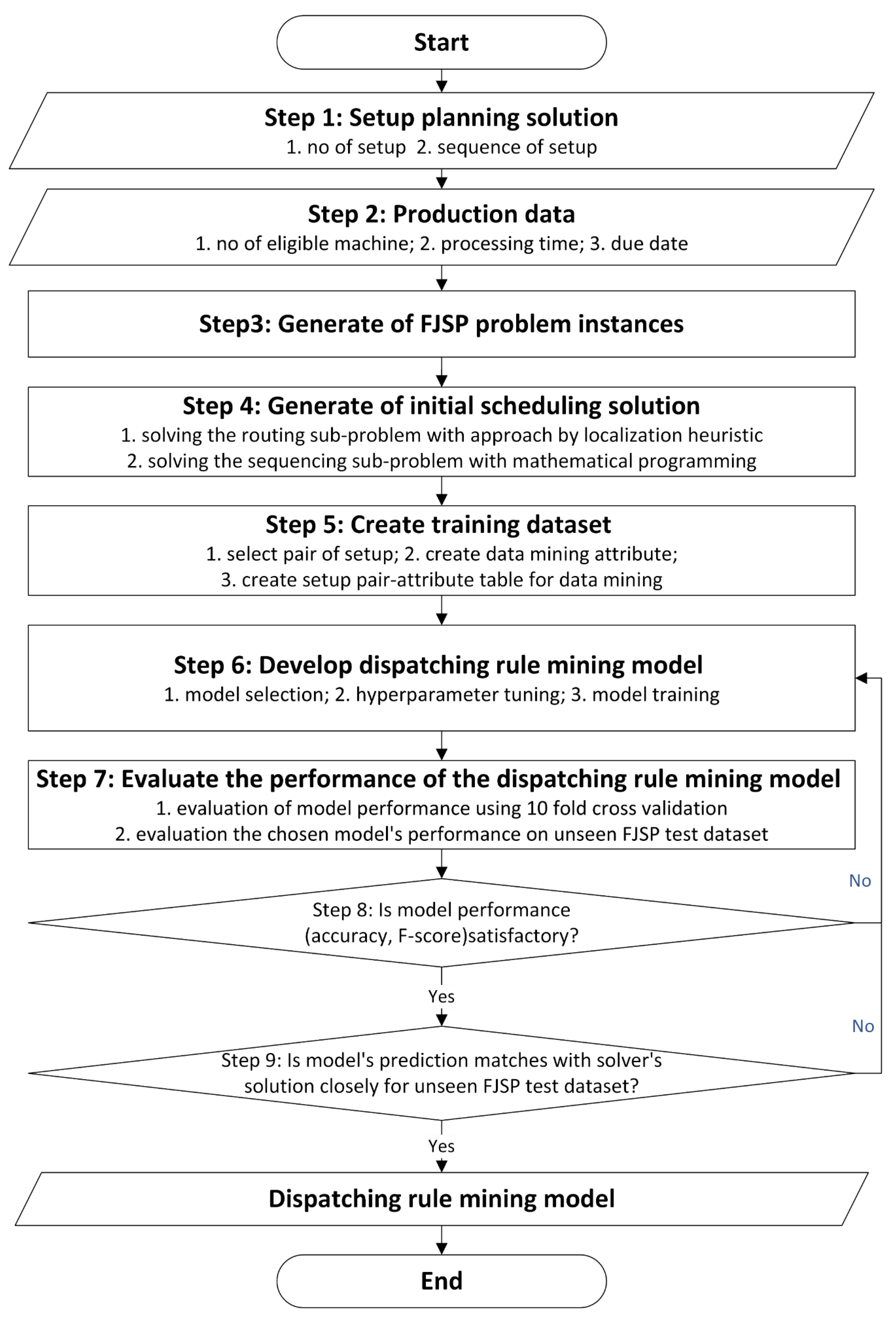
Figure 3.
Process of training dataset generation.
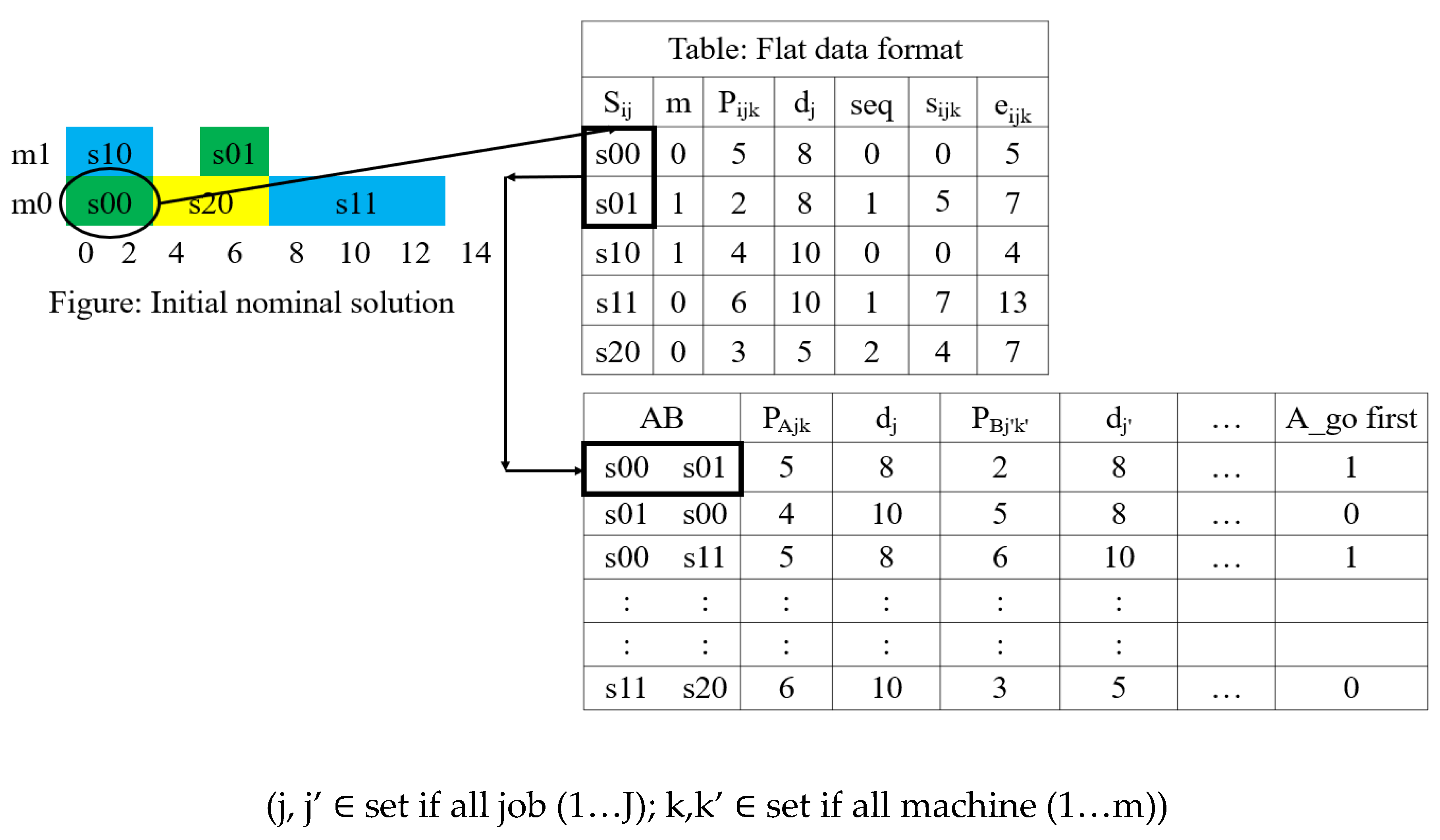
Figure 5.
Gantt chart (a) Case study 1, (b) Case study 2, (c) Case study 3.
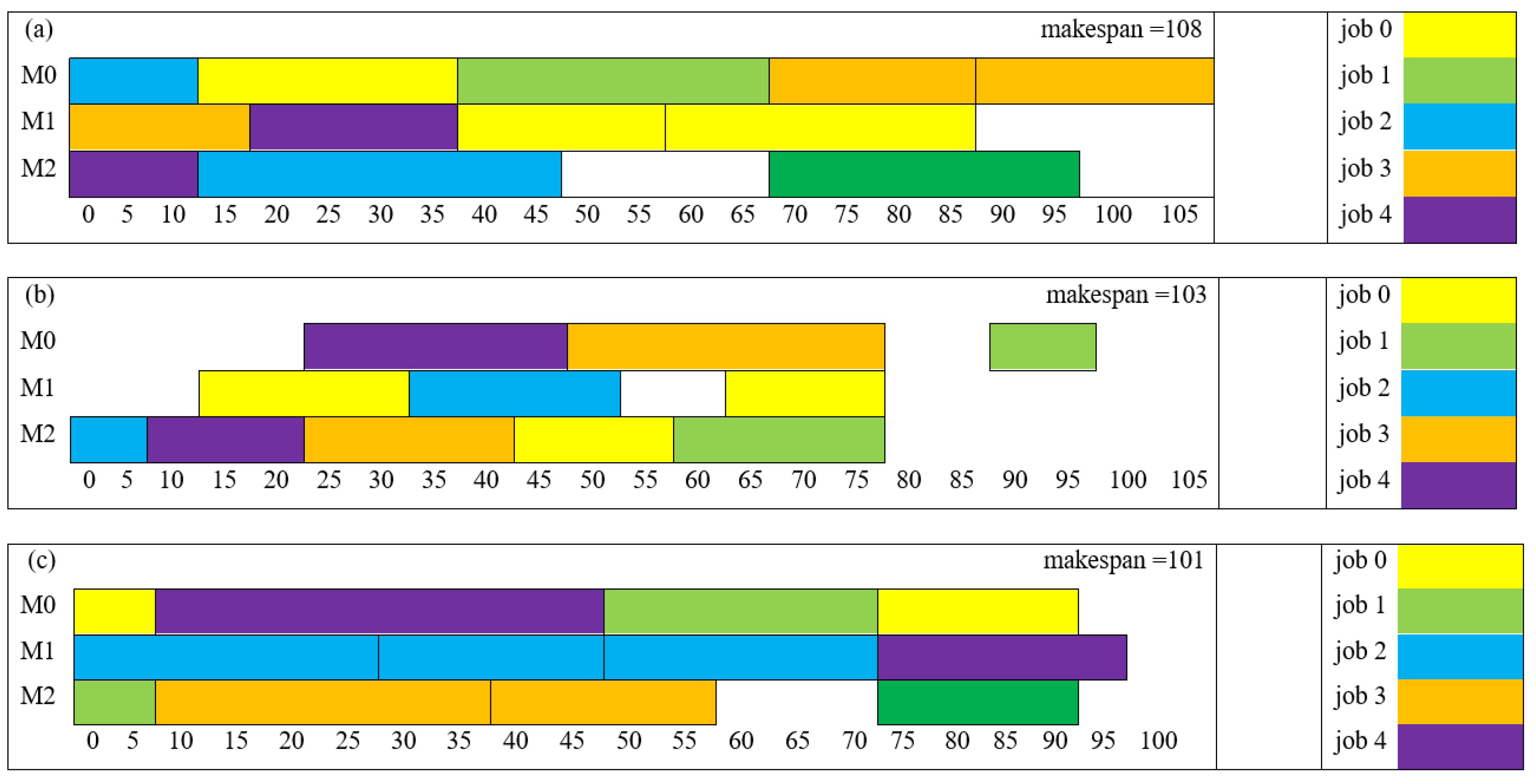
Figure 6.
Predicted sequence of Case study 1.
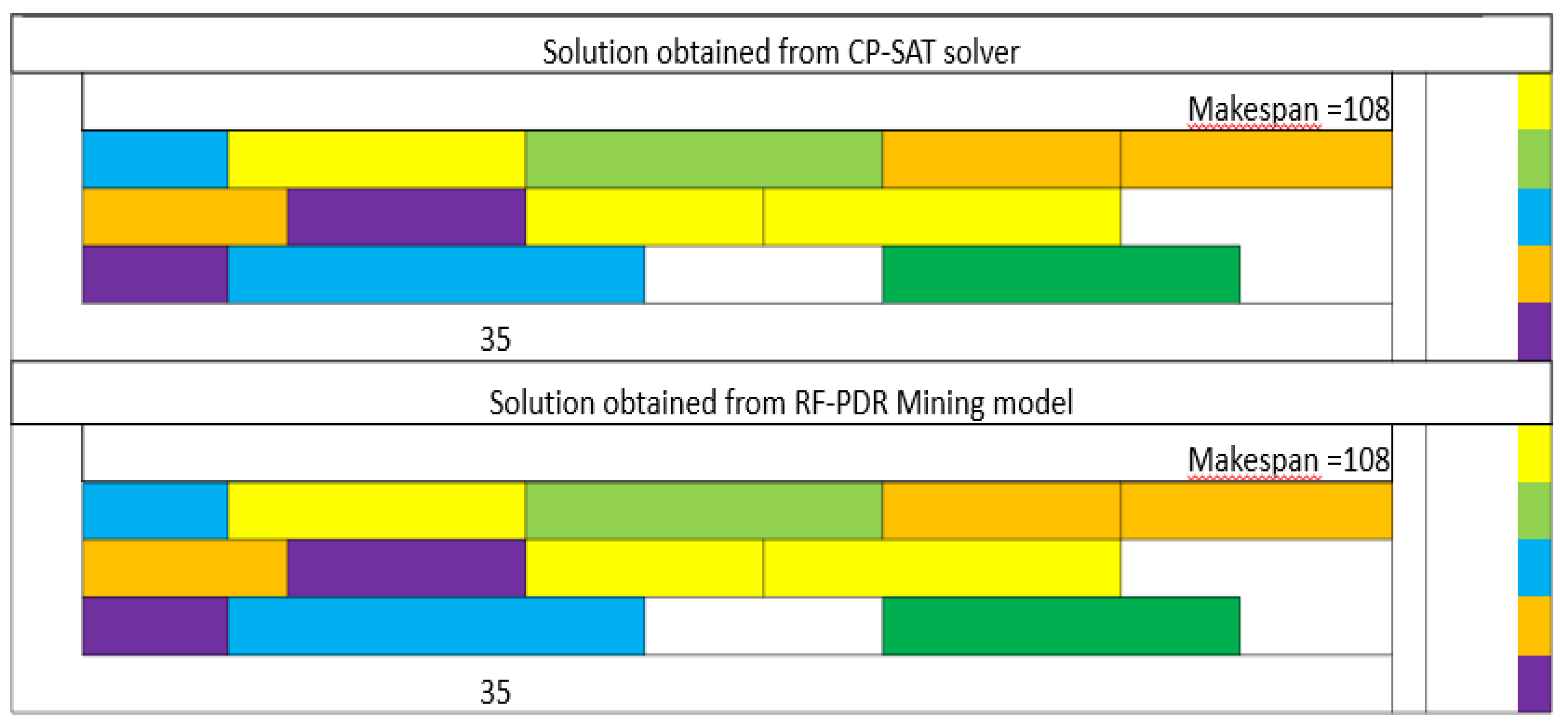
Figure 7.
Predicted sequence of Case study 2.
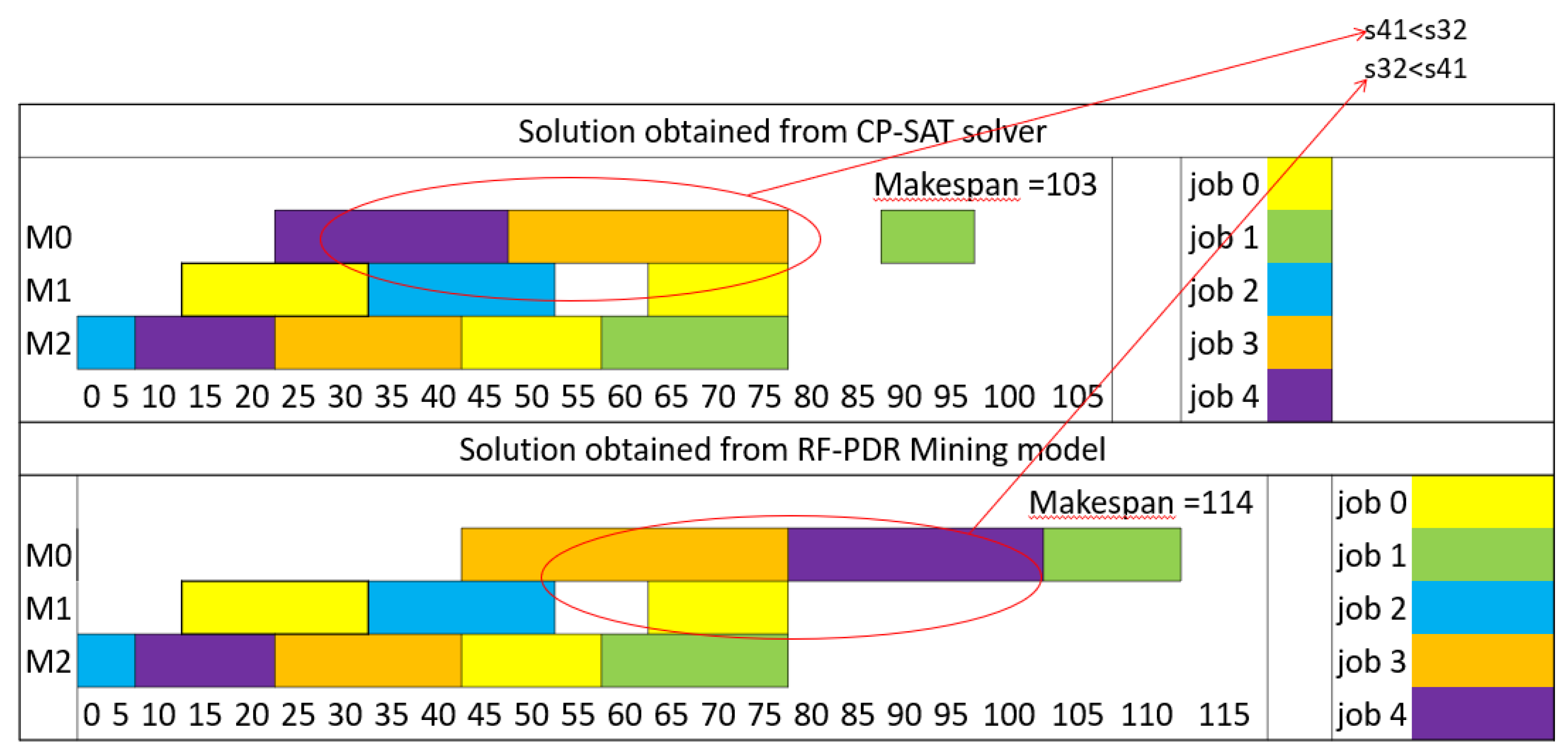
Figure 8.
Predicted sequence of Case study 3.
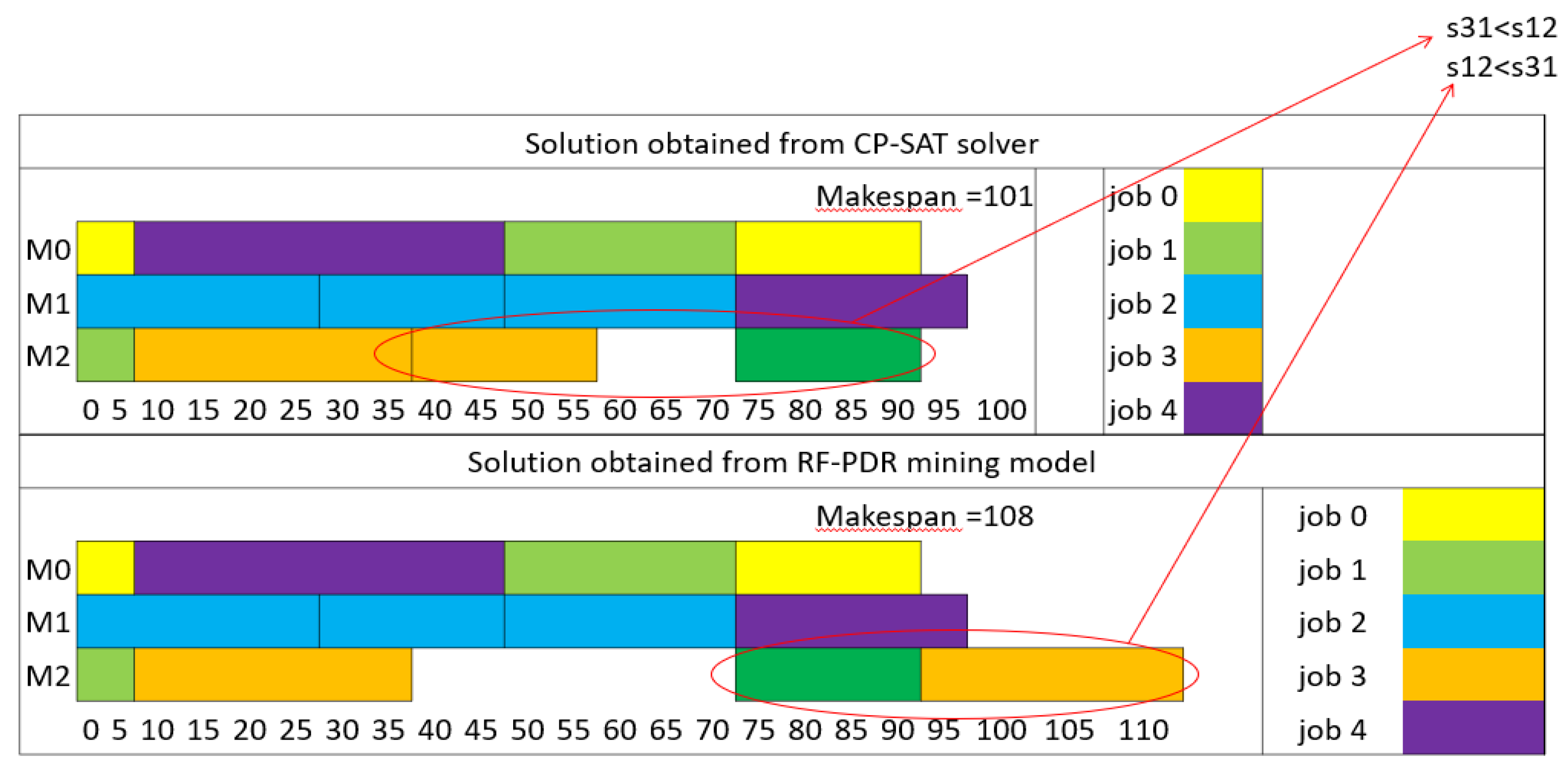
Figure 9.
Time of breakdown.
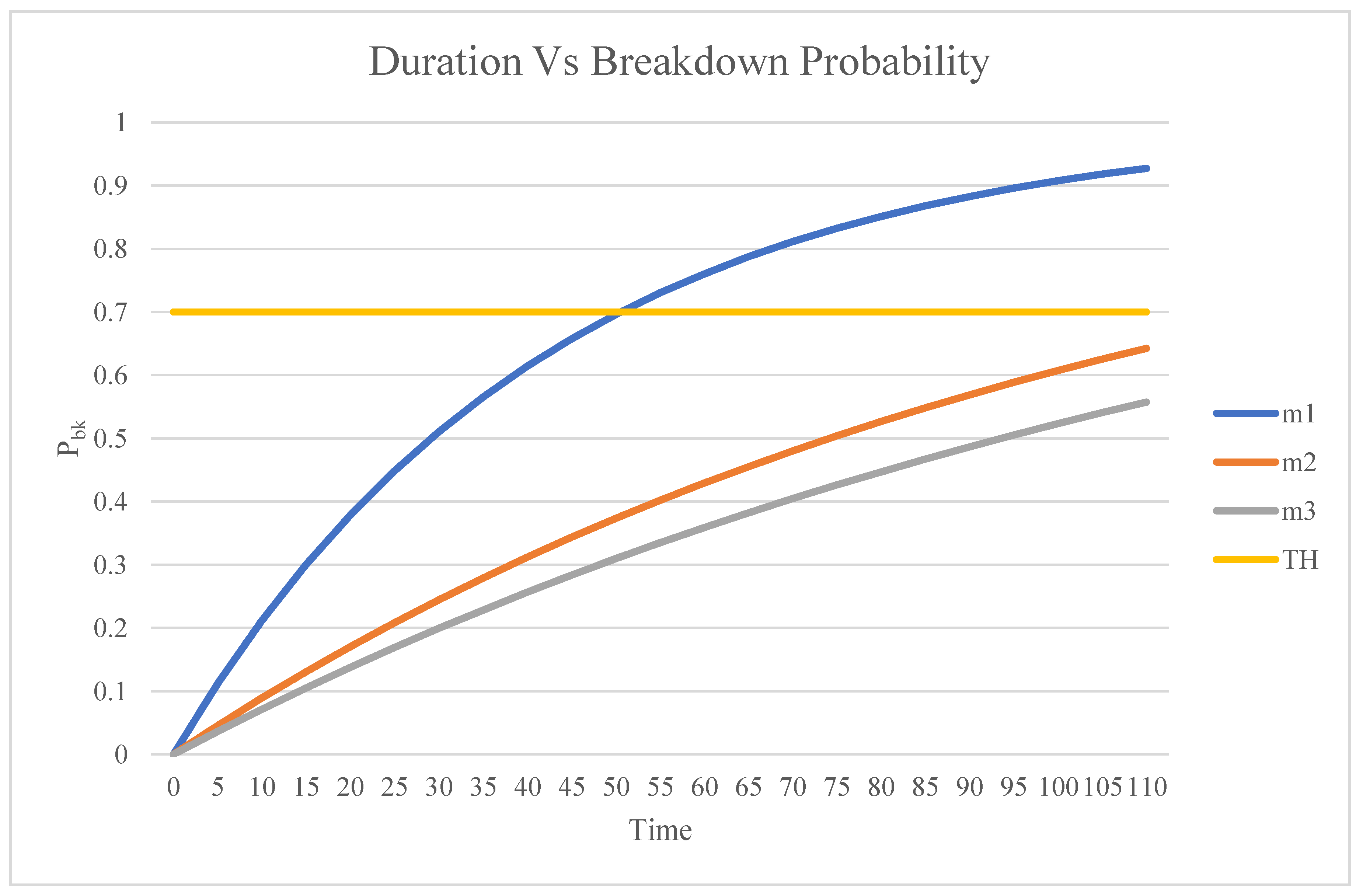
Figure 10.
Rescheduling solution.
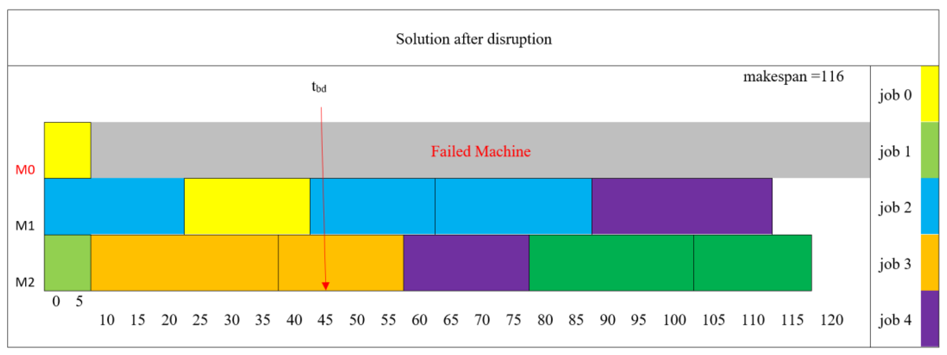
Table 1.
Synthesis of IPPS Research.
| Ref. | j x m | SP | Routing | Sequencing | uncertainty | Obj. | ||||||
| O. Grouping | O. Sequencing | S. Sequencing | O | S | O | S | Static | Dynamic | PP | Scheduling | ||
| (Kumar and Rajotia 2003) | 1 x m | √ | √ | tol, SF | MFT, # Jtk | |||||||
| (Cai, Wang, and Feng 2008) | 1 x m | √ | √ | √ | Ps, #S | |||||||
| (Cai, Wang, and Feng 2009) | 1 x m | √ | √ | √ | C, Mutl | Cmax | ||||||
| (Wang et al. 2010) | 1 x m | √ | √ | √ | C, Mutl | Cmax | ||||||
| (Wang et al. 2010) | 1 x m | √ | √ | √ | C, Mutl | Cmax | ||||||
| (P. Mohapatra, Benyoucef, and Tiwari 2013b) | 1 x m | √ | √ | √ | C, Mutl | Cmax | ||||||
| (P. Mohapatra, Benyoucef, and Tiwari 2013a) | 1 x m | √ | √ | √ | Mutl | Cmax | ||||||
| (Priyabrata Mohapatra, Nanda, and Maji 2015) | 1 x m | √ | √ | √ | C, Mutl | Cmax | ||||||
| (Haddadzade, Razfar, and Zarandi 2016) | n x m | √ | √ | √ | C, Mutl, #S | Cmax | ||||||
| (Barzanji, Naderi, and Begen 2020) | n x m | √ | √ | √ | Cmax | |||||||
| (X. Wu and Li 2021) | n x m | √ | √ | √ | Cmax | |||||||
| (Ming and Mak 2000) | √ | √ | √ | #S | ||||||||
| (Joshi, Kumar, and Sharma 2008) | √ | √ | √ | #S | ||||||||
| (Hua-Bing 2015) | 1 x m | √ | √ | √ | √ | |||||||
| (W. Wu et al. 2020) | 1 x m | √ | √ | √ | C, Es | |||||||
| (Ameer and Dahane 2023) | 1 x 1 (reconfigurable) | √ | √ | C | ||||||||
| (Phung et al. 2017) | √ | C | ||||||||||
| (Hazarika et al. 2011) | √ | √ | √ | |||||||||
| (Hajimiri et al. 2017) | √ | √ | √ | #S | ||||||||
| (Davood Manafi and Nategh 2020) | 1 x m | √ | √ | √ | √ | √ | C | |||||
| (D. Manafi and Nategh 2021) | √ | √ | √ | |||||||||
| (D. Manafi and Nategh 2023) | 1 x m | √ | √ | √ | √ | C | ||||||
| (Y. Zhang et al. 2022) | √ | √ | C | |||||||||
| Current Work | n x m | √ | √ | √ | √ | √ | √ | #S | Cmax | |||
(j = job, m = machine, O = operation, S= setup, #S = no of setup, C= cost, Mutl= machine utilization, tol= tolerance, SF= surface finish, Ps= Part stability, MFT= mean flow time, # Jtk = no of tardy job, Cmax= makespan, Es= stacking error).
Table 2.
Algorithm for solving routing subproblem.
| Input: | FJSP problem instance | |
| Output: | Route of Jobs | |
| For index in range(length_input): | ||
| row = random_select | # Get the current row by random selection | |
| get row_min get min_column_index |
# assign setup in machine with min_pt | |
| for i in range(index+1, len(length_input)): | ||
| row_val += row_min | #Add the minimum value to the subsequent rows in the same column | |
| End For | ||
| End For |
Table 3.
Approach by localization.
| M1 | M2 | M3 | M1 | M2 | M3 | M1 | M2 | M3 | … | M1 | M2 | M3 | |||
| s11 | 7 | 6 | 4 | 7 | 6 | 5 | 11 | 6 | 5 | 7 | 6 | 4 | |||
| s12 | 4 | 8 | 5 | 4 | 8 | 6 | 4 | 8 | 6 | 4 | 8 | 5 | |||
| s13 | 9 | 5 | 4 | 9 | 5 | 5 | 13 | 5 | 5 | 9 | 5 | 4 | |||
| s21 | 2 | 5 | 1 | 2 | 5 | 1 | 6 | 5 | 1 | 2 | 5 | 1 | |||
| s22 | 4 | 6 | 8 | 4 | 6 | 9 | 8 | 6 | 9 | 4 | 6 | 8 |
Machine workload updates are in boldface; highlighted cells show the final assigned machines (solution of the routing problem).
Table 4.
Considered attributes for rule mining.
| Type | Feature/attributes | Notation |
| Raw | processing time of setup A | p_A |
| processing time of setup B | p_B | |
| due data of the A | d_A | |
| due data of the B | d_B | |
| Constructed | if processing time of A is higher than B (categorical) | p_A>B |
| if due date of A is higher than B (categorical) | d_A>B | |
| processing time difference | p_A-B | |
| Due date difference | d_A-B | |
| if A & B has precedence relationship (categorical) | Zii'j | |
| if A precedes B (categorical) | Zij>Zi'j | |
| if A and B processed on same machine (categorical) | xii'k |
Table 6.
Initial nominal solution in flat data format.
| Sij | k | Pijk | dj | seq | sijk | eijk |
| s00 | 0 | 23 | 49.2 | 1 | 16 | 39 |
| s01 | 1 | 21 | 49.2 | 2 | 39 | 60 |
| s02 | 1 | 27 | 49.2 | 3 | 60 | 87 |
| s10 | 0 | 31 | 44.4 | 2 | 39 | 70 |
| s11 | 2 | 29 | 44.4 | 2 | 70 | 99 |
| s20 | 0 | 16 | 45.2 | 0 | 0 | 16 |
| s21 | 2 | 30 | 45.2 | 1 | 18 | 48 |
| s30 | 1 | 18 | 48 | 0 | 0 | 18 |
| s31 | 0 | 19 | 48 | 3 | 70 | 89 |
| s32 | 0 | 19 | 48 | 4 | 89 | 108 |
| s40 | 2 | 18 | 42.8 | 0 | 0 | 18 |
| s41 | 1 | 21 | 42.8 | 1 | 18 | 39 |
Sij = Setup ID, k = Assigned machine, Pijk = Processing time of Sij on k, dj = Due date of job j,. seq = Sequence of Sij on k, sijk = Start time of Sij on k, eijk = End time of Sij on k
Table 7.
Normalized scores for each learning algorithm by metrics (average over 5-folds).
| Model | Combinations | ACC | FSC | ROC | APR | REC | RMS | MXE | MEAN | TIME |
| RF (num_tree, num_Features) | 100,1 | 0.643 | 0.570 | 0.593 | 0.591 | 0.609 | 0.500 | 0.333 | 0.548 | 0.980 |
| 100,6 | 0.738 | 0.670 | 0.701 | 0.705 | 0.696 | 0.375 | 0.251 | 0.591 | 0.927 | |
| 100,11 | 0.810 | 0.748 | 0.691 | 0.773 | 0.783 | 0.188 | 0.186 | 0.597 | 0.950 | |
| 300,1 | 0.857 | 0.783 | 0.845 | 0.864 | 0.739 | 0.250 | 0.137 | 0.639 | 2.735 | |
| 300,6 | 0.857 | 0.783 | 0.845 | 0.864 | 0.739 | 0.250 | 0.137 | 0.639 | 2.735 | |
| 300,11 | 0.925 | 0.890 | 0.907 | 0.919 | 0.917 | 0.108 | 0.078 | 0.643 | 2.353 | |
| 500,1 | 0.952 | 0.913 | 0.948 | 0.909 | 0.913 | 0.125 | 0.069 | 0.690 | 4.324 | |
| 500,6 | 1.000 | 0.957 | 1.000 | 1.000 | 1.000 | 0.063 | 0.029 | 0.721 | 4.586 | |
| 500,11 | 1.000 | 1.000 | 1.000 | 1.000 | 1.000 | 0.000 | 0.000 | 0.714 | 4.703 | |
| KNN | k=1 | 0.833 | 0.714 | 1.000 | 1.000 | 0.875 | 0.750 | 1.000 | 0.882 | 0.000 |
| k=20 | 0.667 | 0.714 | 0.706 | 0.833 | 0.625 | 0.750 | 0.902 | 0.742 | 0.006 | |
| k=50 | 0.500 | 0.429 | 0.412 | 0.500 | 0.375 | 0.875 | 0.902 | 0.570 | 0.009 | |
| k=80 | 0.500 | 0.429 | 0.412 | 0.500 | 0.375 | 0.875 | 0.902 | 0.570 | 1.000 | |
| SVM (kernel, coeff) | ‘linear’, ’scale’ | 0.500 | 0.286 | 0.412 | 0.500 | 0.375 | 0.875 | 0.853 | 0.543 | 0.067 |
| ‘rbf’, ’scale’ | 0.500 | 0.286 | 0.412 | 0.333 | 0.375 | 0.938 | 0.833 | 0.525 | 0.067 | |
| ‘poly’, ’scale’ | 0.333 | 0.286 | 0.412 | 0.333 | 0.000 | 0.938 | 0.804 | 0.444 | 0.079 | |
| ‘linear’, ’auto’ | 0.333 | 0.286 | 0.412 | 0.333 | 0.250 | 0.875 | 0.804 | 0.470 | 0.070 | |
| ‘rbf’, ’auto’ | 0.333 | 0.286 | 0.412 | 0.333 | 0.250 | 0.938 | 0.804 | 0.479 | 0.061 | |
| ‘poly’, ’auto’ | 0.333 | 0.143 | 0.118 | 0.333 | 0.250 | 0.938 | 0.706 | 0.403 | 0.055 | |
| ‘linear’, 0.001 | 0.333 | 0.143 | 0.118 | 0.000 | 0.250 | 0.938 | 0.735 | 0.360 | 0.070 | |
| ‘rbf’, 0.001 | 0.333 | 0.143 | 0.118 | 0.167 | 0.250 | 0.938 | 0.716 | 0.381 | 0.070 | |
| ‘poly’, 0.001 | 0.167 | 0.143 | 0.118 | 0.167 | 0.250 | 1.000 | 0.706 | 0.364 | 0.076 | |
| ‘linear’, 0.01 | 0.167 | 0.143 | 0.118 | 0.167 | 0.250 | 1.000 | 0.696 | 0.363 | 0.073 | |
| ‘rbf’, 0.01 | 0.167 | 0.000 | 0.118 | 0.167 | 0.125 | 1.000 | 0.676 | 0.322 | 0.070 | |
| ‘poly’, 0.01 | 0.167 | 0.100 | 0.118 | 0.167 | 0.125 | 1.000 | 0.667 | 0.335 | 0.070 | |
| ‘linear’, 1 | 0.167 | 0.100 | 0.118 | 0.000 | 0.125 | 1.000 | 0.657 | 0.309 | 0.055 | |
| ‘rbf’, 1 | 0.167 | 0.086 | 0.059 | 0.167 | 0.150 | 1.000 | 0.645 | 0.325 | 0.052 | |
| ‘poly’, 1 | 0.000 | 0.143 | 0.059 | 0.000 | 0.125 | 1.000 | 0.637 | 0.281 | 0.052 | |
| NB | 0.167 | 0.000 | 0.118 | 0.000 | 0.125 | 1.000 | 0.627 | 0.291 | 0.061 | |
| LR (tol) | tol = 0.0001 | 0.167 | 0.000 | 0.118 | 0.000 | 0.125 | 1.000 | 0.618 | 0.290 | 0.064 |
| tol = 0.001 | 0.167 | 0.000 | 0.000 | 0.000 | 0.125 | 1.000 | 0.608 | 0.271 | 0.061 | |
| tol = 1 | 0.083 | 0.000 | 0.000 | 0.000 | 0.125 | 1.000 | 0.598 | 0.258 | 0.061 | |
| tol = 100 | 0.083 | 0.029 | 0.000 | 0.000 | 0.125 | 1.000 | 0.588 | 0.261 | 0.067 | |
| tol = 10000 | 0.083 | 0.026 | 0.000 | 0.000 | 0.125 | 1.000 | 0.582 | 0.267 | 0.061 |
Table 8.
Comparison of mined dispatching rule with SPT and EDD dispatching rule.
| instance | jxk | i | Cmax | ||||
| RF-PDR | SPT | % dev | EDD | % dev | |||
| FJSP5_C1 | 5x3 | 2-3 | 108 | 169 | 36% | 166 | 35% |
| FJSP5_C2 | 5x3 | 2-3 | 114 | 166 | 31% | 198 | 42% |
| FJSP5_C3 | 5x3 | 2-3 | 108 | 141 | 23% | 169 | 36% |
Table 9.
Initial nominal solution for case study 3 in a flat data format.
| setup_id | Eligible machine | Solution | ||||
| m0 | m1 | m2 | Assigned mid | start | end | |
| s00 | 10 | 13 | 0 | 0 | 10 | |
| s01 | 20 | 12 | 23 | 0 | 75 | 95 |
| s10 | 25 | 11 | 2 | 0 | 11 | |
| s11 | 27 | 18 | 20 | 0 | 48 | 75 |
| s12 | 44 | 26 | 15 | 2 | 75 | 90 |
| s20 | 47 | 30 | 27 | 1 | 0 | 30 |
| s21 | 27 | 18 | 1 | 30 | 48 | |
| s22 | 25 | 29 | 1 | 48 | 73 | |
| s30 | 35 | 22 | 18 | 2 | 11 | 40 |
| s31 | 19 | 27 | 0 | 2 | 40 | 58 |
| s40 | 38 | 23 | 0 | 10 | 48 | |
| s41 | 38 | 28 | 29 | 1 | 73 | 101 |
Table 10.
Setup status after machine breakdown.
| setup_id | current eligible machine | solution | status | |||
| m1 | m2 | assigned m_id | start | end | ||
| s01 | 12 | 23 | - | - | - | Interrupted |
| s11 | 18 | 20 | - | - | - | Interrupted |
| s40 | 23 | - | - | - | Interrupted | |
| s21 | 18 | 1 | 30 | 48 | Unfinished | |
| s22 | 25 | 29 | 1 | 48 | 73 | Unfinished |
| s41 | 28 | 29 | 1 | 73 | 101 | Unfinished |
| s12 | 26 | 15 | 2 | 75 | 90 | Unfinished |
| s31 | 27 | 18 | 2 | 40 | 58 | Unfinished |
Table 11.
Updated routing of interrupted setups.
| setup_id | m1 | m2 |
| s01 | 12 | 23 |
| s11 | 18 | 20 |
| s40 | 23 |
Table 12.
Comparative Analysis with Classical Dispatching Rules.
| Cmax | RM % | SM | |
| RF-PDR | 116 | 12.93 | 25.8 |
| SPT | 144 | 33.33 | 21.4 |
| EDD | 152 | 40.7 | 52.6 |
Disclaimer/Publisher’s Note: The statements, opinions and data contained in all publications are solely those of the individual author(s) and contributor(s) and not of MDPI and/or the editor(s). MDPI and/or the editor(s) disclaim responsibility for any injury to people or property resulting from any ideas, methods, instructions or products referred to in the content. |
© 2025 by the authors. Licensee MDPI, Basel, Switzerland. This article is an open access article distributed under the terms and conditions of the Creative Commons Attribution (CC BY) license (http://creativecommons.org/licenses/by/4.0/).
Copyright: This open access article is published under a Creative Commons CC BY 4.0 license, which permit the free download, distribution, and reuse, provided that the author and preprint are cited in any reuse.


