
Submitted:
08 June 2025
Posted:
10 June 2025
You are already at the latest version
Abstract
This study analyzes the financial returns of globally operating transportation and logistics firms, examining the impact of Environmental, Social, and Governance (ESG) factors and broader market dynamics. Utilizing a dataset of 14 firms over a decade (2012–2021), the research first employs panel data regressions to quantify the influence of ESG scores and established asset pricing factors on excess returns. Second, market-level time series analysis, specifically Vector Autoregression (VAR) and GARCH modeling, explores the dynamic interrelationships between market returns and aggregate ESG performance. Finally, advanced machine learning classifiers (Random Forest, XGBoost) predict future excess return direction, identifying key predictive features through importance and SHAP analysis. Findings reveal that traditional market factors significantly influence firm returns, while ESG performance demonstrates a nuanced, often negative association. Machine learning models show high predictive power, highlighting critical financial and environmental determinants. These results are useful for investors seeking to optimize risk-adjusted returns, industry stakeholders making strategic investments in sustainability and technology, and policymakers developing resilient and green logistics frameworks.
Keywords:
transportation logistics
; ESG
; financial performance
; asset pricing
; panel data
; vector autoregression
; machine learning
; predictive analytics
; sustainability
; supply chain
1. Introduction
The transportation and logistics sector stands as a foundational pillar of the global economy, currently undergoing profound and rapid transformation. This dynamic shift is propelled by significant advancements in areas such as hyperautomation, the pervasive influence of artificial intelligence (AI) and machine learning (ML), an escalating imperative for sustainability, widespread digitalization, and evolving consumer and regulatory demands [1]. These transformative trends, encompassing the adoption of hyperautomation and robotics, the development of self-learning and predictive transport management systems, and the crucial integration of sustainability and green logistics, are fundamentally reshaping the industry landscape. Such developments underscore the urgent need for high-impact research to precisely understand their tangible financial implications for firms operating within this vital sector [1,2]. This study specifically aims to contribute to developing pragmatic solutions to the significant challenges faced by contemporary organizations and society by empirically linking these transformative trends to measurable financial outcomes.
There exists a compelling need for rigorous, high-impact research to ascertain how these transformative trends in transportation and logistics, particularly the increasing integration of sustainability (ESG) imperatives and the rapid pace of technological adoption, translate into concrete financial performance for firms within this sector. The problem is significant because it directly addresses the core strategic challenge of balancing profitability with environmental responsibility and technological advancement in a globally critical industry, thereby influencing investment decisions, refining operational strategies, and shaping effective policy formulation [3,4].
Existing academic literature often examines specific aspects of financial performance, the impacts of ESG, or the implications of technological advancements within the transportation and logistics industry in isolation. A notable research gap persists in comprehensive empirical studies that integrate established financial asset pricing models, such as the Fama-French framework, with advanced analytical methodologies, including panel data techniques and cutting-edge machine learning approaches. Such a multi-faceted analysis is crucial for a holistic assessment of the intertwined effects of ESG factors, broader market dynamics, and the sector’s pervasive transformative trends on firm financial performance. While this study leverages widely recognized datasets (Bloomberg, Refinitiv, triangulated with Sustainalytics, MSCI, and Morningstar ESG-risk-rating data, established asset pricing factors, and historical stock prices), its originality stems from its significantly innovative methodological approach. This innovation lies in the integrated application of panel data econometrics, time series analysis (specifically VAR/GARCH), and advanced machine learning techniques (Random Forest, XGBoost with SHAP interpretability). This unique combination allows for a joint analysis of the complex interplay of financial market factors, ESG performance, and the dynamics of a sector undergoing profound technological and sustainable transformation. This triangulation of methods provides a richer, more nuanced understanding of the financial drivers and their predictive power, moving beyond isolated analyses and offering new, significant insights that extend beyond merely replicating existing knowledge in a highly relevant industry that faces distinctive operational and regulatory challenges [5,6].
This study is guided by the following research questions:
- To what extent do established asset pricing factors explain the excess returns of transportation and logistics firms?
- How do firm-level ESG scores (overall and decomposed components) influence the excess returns of these firms?
- What are the dynamic relationships between market returns and market-level ESG factors in the transportation and logistics sector?
- Can machine learning models effectively predict the direction of future excess returns for these firms, and what are the most influential predictive features?
This study offers substantial practical and theoretical contributions. From a practical standpoint, it provides investors with granular insights into risk-adjusted returns and sustainability considerations specific to the transportation and logistics sector. For industry practitioners, the findings highlight critical trends that demand strategic investment, thereby fostering the connection between theory and practice by identifying financially impactful aspects of sustainability and technological adoption [7,8]. For policymakers, the research informs the development of effective regulatory frameworks designed to promote sustainable and resilient logistics. Theoretically, this study generates new and significant information, leading to a notable theoretical contribution by refining the understanding of multi-factor asset pricing and the ESG-finance nexus within a dynamic industrial context. Furthermore, it contributes to developing solutions to the significant challenges faced by contemporary organizations by providing empirical evidence for navigating complex trade-offs between profitability, environmental responsibility, and technological innovation, thereby addressing pressing societal challenges.
The remainder of this paper is organized as follows. Section 2 covers the theoretical foundation as well as a thorough analysis of relevant literature. Section 3 explains the approach, which includes data collection, preprocessing, and the econometric and machine learning models used. Section 4 contains the empirical findings, including tables and figures from the analysis. Section 5 presents a discussion of the findings, meticulously addressing each study topic and connecting them to broader implications. Finally, Section 6 summarizes the study’s findings, discusses its contributions, and offers areas for future research.
2. Theoretical Framework and Literature Review
2.1. Overview of Key Trends in Transportation and Logistics
The transportation and logistics sector is currently characterized by a set of transformative trends that are profoundly reshaping its landscape [1]. These include the widespread adoption of Hyper-automation and Robotics, which integrate AI, robotics, and IoT to optimize processes, leading to real-time decision-making and reduced operational costs. Self-learning and Predictive Transport Management systems increasingly utilize AI and big data for route optimization, demand prediction, and fuel efficiency, thereby enhancing supply chain flexibility and resilience. Sustainability and Green Logistics are driving the accelerated adoption of electric commercial vehicles and the integration of circular logistics models, placing environmental goals at the core of logistics strategies [9,10]. Digitalization and Real-Time Visibility are key drivers, leveraging telemetry, IoT, and advanced analytics for enhanced tracking, transparency, and process automation; real-time visibility (Visibility 2.0) is becoming a baseline expectation. The effective leveraging of Big Data and Predictive Analytics is now essential for demand forecasting, operational optimization, and disruption management. Furthermore, logistics companies are investing in API-Based and Ecosystem Integration to enable seamless data exchange and collaborative supply chain ecosystems. Achieving Supply Chain Agility and Resilience is critical for responding effectively to disruptions, labor shortages, and changing market conditions. Circular and Resource-Efficient Logistics models, emphasizing resource reuse and waste reduction, are gaining traction as companies prioritize sustainability and cost efficiency. Other notable trends encompass enhanced Security and Advanced Payment Solutions, addressing global Labor and Talent Management challenges, navigating Regulatory and Geopolitical Risks, and advancements in fleet management systems with AI-based predictions and the growth of digital freight marketplaces [11,12]. These trends collectively reshape the operational, strategic, and financial landscapes of the sector, demanding rigorous, high-impact research.
2.2. Theoretical Foundations
Supply Chain Management (SCM) theory, initially formulated by Keith Oliver in 1982, established a framework for integrating procurement, production, distribution, and logistics into a holistic system aimed at creating value and enhancing efficiency [13]. The contemporary evolution of SCM seamlessly incorporates modern trends such as digitalization, sustainability imperatives, and the pursuit of resilience. For instance, modern SCM frameworks are increasingly embracing digital transformation to optimize supply chain visibility and agility [14], while sustainability considerations drive the widespread adoption of green logistics practices [15]. These integrations significantly impact firm performance by improving operational efficiency, reducing costs, and boosting responsiveness to dynamic market demands.
The asset pricing models developed by Eugene Fama and Kenneth French form a cornerstone for understanding and explaining stock returns in financial markets. Building upon the foundational Capital Asset Pricing Model (CAPM), Fama and French (1993) introduced their influential three-factor model, which incorporates market excess return, a size premium (SMB), and a value premium (HML) to elucidate the cross-section of stock returns. Their subsequent refinement led to the five-factor model in 2015, which further augmented explanatory power by adding profitability (RMW) and investment (CMA) factors [16]. These factors are instrumental in capturing diverse dimensions of risk and return in equity markets, rendering them highly relevant for assessing factor exposure and risk-adjusted returns for firms within the transportation and logistics sector [17].
Machine learning theory provides the fundamental principles underpinning advanced algorithms utilized for predictive analytics. Leo Breiman’s seminal work on Random Forest in 2001 introduced an ensemble learning method that constructs multiple decision trees and aggregates their predictions, proving to be robust against overfitting and highly capable of discerning complex, non-linear relationships within data [18]. Building on the strengths of gradient boosting, Tianqi Chen and Carlos Guestrin’s development of XGBoost in 2016 offered a highly optimized algorithm that often delivers superior predictive performance, particularly in handling sparse data and large datasets [19]. These sophisticated tools are eminently suitable for financial prediction, risk management, and operational optimization within logistics, enabling the complex modeling of relationships among market dynamics, ESG factors, and financial performance, often surpassing the capabilities of traditional econometric models [20].
Open Innovation, a concept pioneered by Henry Chesbrough (2003), underscores the strategic importance for organizations to leverage both internal and external ideas, as well as internal and external paths to market [21]. This theoretical framework holds particular relevance for technologically advanced sectors such as logistics, where rapid advancements in AI, IoT, and API integration necessitate collaborative approaches. Transportation firms can strategically harness external expertise through participation in digital marketplaces and by forming partnerships for developing green technologies, thereby fostering innovation and achieving a competitive advantage by adapting effectively to emergent industry trends [22].
The Blue Ocean Strategy, conceptualized by W. Chan Kim and Renée Mauborgne (2005), advocates for creating uncontested market space, rendering competition irrelevant, typically through radical innovation and novel value creation [23]. Within the dynamic context of the transportation and logistics sector, a steadfast pursuit of sustainability and the adoption of advanced technology can empower firms to carve out new market territories or fundamentally redefine existing ones. For instance, pioneering new circular logistics services or developing highly automated, transparent supply chains can serve as powerful differentiators, enabling firms to move beyond traditional cost-based competition and establish new, sustainable value propositions [24].
2.3. Literature Review
2.3.1. ESG and Financial Performance
The relationship between Environmental, Social, and Governance (ESG) performance and financial returns is a subject of extensive academic inquiry, characterized by diverse and sometimes contradictory findings across various industries and geographical contexts [25]. Within the transportation and logistics sector specifically, the growing significance of ESG considerations is increasingly recognized [3,4]. Recent research suggests that incorporating “green” practices can serve as an instrument for enhancing firm value, particularly for US transport and logistics companies, although this relationship can be context-dependent and influenced by specific ESG risk profiles [2]. Other studies delve into how corporate branding within the logistics sector reflects ESG programs and impacts overall performance, while some explore the role of factors like board gender diversity in the sustainability and financial performance of transport and logistics firms, often drawing upon stakeholder theory [26,27,28]. Broadly, while there is a consensus on the increasing relevance of ESG, the precise mechanisms and resulting financial outcomes remain a complex area requiring nuanced analysis, which underscores the importance of sector-specific studies like the present one [29]. This section ensures adequate reference to other work in the field to establish the current state of knowledge.
2.3.2. Emission Categories (Scopes 1, 2, 3) and CO2 in Transport and Logistics
Transportation activities represent a major source of environmental emissions, which are classified into three distinct categories [53]. Scope 1 covers emissions directly generated by company-controlled operations, particularly from their transportation fleet’s fuel usage [9]. Energy purchases for facilities such as distribution centers create Scope 2 emissions through indirect generation. The broader supply chain activities, including contracted carriers and related services, generate Scope 3 emissions, encompassing both upstream and downstream operations [54]. Among greenhouse gases, CO2 emissions from fuel consumption represent the most significant environmental impact in transportation [10]. In response to emission concerns, companies are transitioning to electric vehicles and implementing environmentally conscious logistics practices [9,10]. Contemporary research examines methods to optimize emissions across these categories, considering both environmental benefits and cost implications [7,8]. These emission classifications serve as essential metrics for developing effective sustainability strategies in logistics operations.
2.3.3. Advancements in Technology and Digitalization Across Logistics and Finance
The transportation and logistics sector is currently undergoing a profound transformation, propelled by the swift integration of cutting-edge technologies and pervasive digitalization. This shift is fundamentally reshaping existing operational paradigms and introducing novel financial considerations. In transport management, artificial intelligence (AI) is being used more and more for predictive analytics, sophisticated route optimization, and demand forecasting. These applications have resulted in notable increases in efficiency and significant cost savings [30,31]. Real-time tracking and improved visibility for assets, vehicles, and goods are made possible by the Internet of Things (IoT), which improves operational command and supply chain transparency [32,33]. Blockchain technology presents a secure, unalterable, and distributed ledger system for transactions, which boosts trust and helps mitigate fraud within logistics operations. Furthermore, this technology is being combined with concepts such as Digital Twins to facilitate more effective monitoring and optimization of vehicle fleets and broader logistics processes [34,35]. Digital Twins, which are virtual representations of physical assets or systems, are experiencing considerable momentum for sophisticated scenario planning and process refinement across diverse applications, including container shipping and road transport, despite the associated implementation costs [36,37]. Emerging digital initiatives, such as the Metaverse and Extended Reality (XR) applications, show considerable promise for revolutionizing training methodologies, collaborative design, and immersive visualization experiences within logistics; however, their direct quantifiable financial impact remains an active area of investigation [38].
Additional digital advancements comprise automated customs procedures, highly sophisticated big data management systems, scalable cloud computing solutions, and advanced analytics tools specifically designed to support enhanced decision-making [20,39,40,41]. Taken together, these technologies are instrumental in strengthening supply chain resilience, streamlining operational workflows, and uncovering novel business opportunities, thereby fundamentally altering the financial landscape of the sector [14,42,43,44,45,46]. This discussion intentionally incorporates insights from recent academic discourse to ensure its relevance to contemporary industry debates.
2.3.4. AI/ML in Financial and Logistics Prediction
The application of Artificial Intelligence (AI) and Machine Learning (ML) has witnessed a rapid expansion across both financial forecasting and logistics optimization domains [20]. In finance, ML algorithms are strategically employed for predictive modeling of stock prices, risk management, and portfolio optimization, often demonstrating superior performance over traditional econometric models by capturing non-linear relationships and intricate interactions within large datasets [49]. Within the realm of logistics, AI and ML are pivotal to the implementation of hyper-automation, the development of self-learning transport management systems, and the creation of smart urban transport solutions, enabling precise demand forecasting, optimized route planning, and highly efficient warehouse management [30,32,42,50]. Numerous studies underscore the effectiveness of specific techniques like Random Forest and XGBoost in enhancing supply chain information management through advanced data analysis, intelligent warehousing solutions, and optimized transportation processes [31,51]. This research systematically builds upon this foundation by applying these advanced ML techniques to specifically predict financial performance (excess returns) within the transportation and logistics sector, leveraging feature importance and SHAP values for interpretability. This approach makes a direct contribution to the industry’s “AI-Driven Optimization” and “Data-Driven Decision Making” objectives.
2.3.5. Synthesis and Research Gap
The comprehensive literature review underscores the escalating importance of ESG considerations, the robust explanatory power of established asset pricing factors, and the transformative potential inherent in advanced technologies within the logistics landscape. However, a significant and discernible gap persists in empirical studies that simultaneously integrate all these critical dimensions to analyze firm-level financial performance within the highly dynamic transportation and logistics sector. Previous research often tends to focus on one or two aspects in isolation or relies on less granular and less sophisticated methodologies. This study directly addresses this critical gap by employing a comprehensive, multi-method approach combining advanced panel data econometrics, rigorous time series analysis, and state-of-the-art machine learning techniques to provide a holistic and nuanced understanding of how broader market dynamics, firm-specific ESG performance, and the pervasive technological trends collectively influence the excess returns of transportation and logistics companies [1,5]. The extensive nature of this literature review is intended to align the study with the latest academic discussions and ensure its relevance to contemporary debates in the field.
3. Methodology
3.1. Research Design
This study adopts a quantitative, empirical research design, utilizing a multi-faceted analytical framework that integrates panel data analysis, time series methods, and machine learning techniques. This comprehensive approach is purposefully selected to allow for both explanatory modeling of the underlying determinants of firm financial performance and predictive modeling of future returns, thereby enabling a robust investigation of the research questions articulated. The methods are described in detail to facilitate replication and critical assessment by other researchers.
3.2. Data Collection and Sources
The study’s methodology commenced with careful data collection and identification of reliable sources.
For Sample Selection, the study analyzes a carefully selected sample of 14 unique publicly traded transportation and logistics firms. The data spans an annual period from 2012 to 2021, resulting in a 10-year observation window for each firm. The selection criteria specifically prioritized firms with consistent data availability across the specified timeframe to ensure comparability and consistency of regulatory and economic environments, thus enhancing the credibility of the findings regarding the “countries analyzed.”
Regarding Data Sources, firm-level Environmental, Social, and Governance (ESG) and financial data were primarily obtained from Bloomberg and Refinitiv terminals. To enhance data robustness and allow for cross-validation, these data were triangulated with ESG-risk-rating data from reputable providers such as Sustainalytics, MSCI, and Morningstar. Established asset pricing factor data, encompassing Mkt-RF, SMB, HML, RMW, CMA, RF, and WML, were meticulously sourced from Kenneth French’s data library, a widely recognized and authoritative academic resource.
Variables: This section outlines the specific variables utilized in the study, categorized into dependent and independent types.
For the Dependent Variable, the primary dependent variable is Excess_Return_Firm, which is calculated as the firm’s annual stock return minus the risk-free rate (RF). The rationale for selecting this variable is its established use in financial economics for measuring risk-adjusted performance, allowing for direct comparison with asset pricing models and providing a standard metric for evaluating investment performance.
Turning to the Independent Variables, several distinct categories were included. First, for Asset Pricing Factors, this set includes Mkt-RF (market excess return), SMB (Small Minus Big), RMW (Robust Minus Weak), and WML (Winners Minus Losers - Momentum Factor). Due to empirically observed high multicollinearity between HML (High Minus Low) and CMA (Conservative Minus Aggressive), Principal Component Analysis (PCA) was systematically applied to these two factors. This yielded two orthogonal components, FF_HML_CMA_PC1 and FF_HML_CMA_PC2, which collectively capture their combined variance while effectively mitigating multicollinearity. These factors are selected as empirically established proxies for various dimensions of market, size, value, profitability, investment, and momentum risks, thereby providing a robust baseline for explaining equity returns.
Next, concerning ESG Factors, the core ESG factors analyzed are ESG_score (representing overall ESG performance), Social_score, Gov_score, and Env_score (environmental performance). Recognizing potential interdependencies among these individual ESG sub-scores, PCA was strategically applied to Social_score, Gov_score, and Env_score. This process derived ESG_PC1, a consolidated measure that explains a significant portion of their collective variance while directly addressing the impact of sustainability performance.
To ensure a comprehensive model, various standard Firm-Specific Financial/Operational Controls were included as control variables. These include BVPS (Book Value Per Share), Market_cap (Market Capitalization), Shares (Number of Shares Outstanding), Net_income, PE_RATIO (Price-to-Earnings Ratio), RETURN_ON_ASSET, Total_assets, and QUICK_RATIO. These variables are chosen for their known influence on firm performance, serving to isolate the specific effects attributed to ESG and market factors.
Furthermore, where data availability permitted, additional granular Detailed ESG/Sustainability Controls were considered. These include Scope_1 (direct greenhouse gas emissions), Scope_2 (indirect greenhouse gas emissions), CO2_emissions, Energy_use, Water_use, Water_recycle, Toxic_chem_red (toxic chemical reduction), Injury_rate, Women_Employees, Human_Rights policy presence, Strikes (labor disputes), Turnover_empl (employee turnover), Board_Size, Shareholder_Rights score, Board_gen_div (board gender diversity), Bribery controls, and Recycling_Initiatives. These were included for their potential to provide a more nuanced view of ESG impact, although their direct inclusion in final models depended on data completeness and statistical significance.
For Engineered Features for ML, to enrich the dataset and enhance the predictive power of the machine learning models, several engineered features were meticulously created. These include momentum features (ESG_score_momentum, Social_score_momentum, Gov_score_momentum, Env_score_momentum, and ESG_PC1_momentum), representing year-over-year changes in these ESG metrics. Additionally, industry-adjusted features (ESG_score_adj, Social_score_adj, Gov_score_adj, Env_score_adj, ESG_PC1_adj, Market_cap_adj, RETURN_ON_ASSET_adj, PE_RATIO_adj, Total_assets_adj) were computed by subtracting the industry average from each firm’s value, thereby capturing their relative performance within the sector. These features are specifically engineered to capture dynamic effects and relative performance, significantly enhancing the predictive capabilities of the machine learning models.
A Market-level ESG Factor, Market_ESG_Factor_VW (Value-weighted Market ESG Factor), was constructed by aggregating the ESG scores across all firms in the sample, weighted by their respective market capitalization. This variable was designed to capture aggregate ESG trends within the transportation and logistics sector for use in time series analysis.
Finally, for the machine learning classification task, the Target Variable for ML, Excess_Return_Firm_next_year_Direction, was created as a binary variable. It is assigned a value of 1 if the Excess_Return_Firm in the subsequent year is positive, and 0 otherwise (negative or zero). This binary variable simplifies the prediction task for classification models and provides actionable insights into the likelihood of future positive returns.
3.3. Data Preprocessing
Before analysis, the raw data underwent rigorous preprocessing steps to ensure its quality and suitability for modeling.
For Missing Data Handling, missing values, as initially observed and detailed in Table 1, were systematically addressed using a robust two-stage imputation approach. First, the Multiple Imputation by Chained Equations (MICE) technique was employed for numerical variables, which models each variable with missing values conditional on other variables in the dataset to provide multiple plausible imputations. For any remaining missing values or categorical data, forward fill (ffill) followed by backwards fill (bfill) was applied to propagate the last or next valid observation within each firm’s time series. This comprehensive strategy ensured data completeness for subsequent analyses.
Next, for the Panel Data Setup, the collected firm-level data was meticulously structured as a balanced panel dataset, indexed by Identifier (RIC) (serving as the entity identifier) and Year (serving as the time index). This precise structuring is fundamental for the appropriate application of panel regression models, allowing for the effective capture of both cross-sectional variations among firms and temporal changes over the study period.
Finally, Multicollinearity Diagnostics were performed to mitigate potential multicollinearity among independent variables, particularly within the asset pricing factors and ESG sub-scores. As noted in the Variable section, PCA was strategically applied to highly correlated asset pricing factors (HML and CMA) to form FF_HML_CMA_PC1 and FF_HML_CMA_PC2. Similarly, PCA was applied to the firm-level ESG sub-scores (ESG_score, Social_score, Gov_score, and Env_score) to derive ESG_PC1. The explained variance ratios for these PCA components are presented in Table 2, confirming that they capture the majority of the original variables’ information while significantly reducing collinearity. The VIF scores for the final set of independent variables utilized in the models are presented in Table 3, demonstrating that multicollinearity has been effectively addressed and is well within acceptable limits.
3.4. Econometric Models
Panel regression models were chosen as the primary econometric tool for analyzing firm-level data over time. This approach offered robust insights into financial performance determinants by effectively controlling for unobserved firm-specific heterogeneity that could bias Ordinary Least Squares (OLS) regressions.
The Pooled OLS model served as a baseline, representing a standard linear regression that assumed constant coefficients across all firms and periods, thus ignoring any inherent panel structure. Robust standard errors were applied to address common issues like heteroskedasticity and autocorrelation in financial panel data, ensuring more reliable statistical inference. The Fixed Effects (Within) Model was employed to explicitly control for unobserved, time-invariant firm-specific heterogeneity, justified by the inherent diversity of firms within the transportation and logistics sector (e.g., unique management styles). By differencing out these fixed effects, the model estimated the impact of within-firm changes in independent variables on the dependent variable, providing unbiased coefficient estimates. Robust standard errors consistently ensured hypothesis test validity. The Random Effects Model offered an alternative to Fixed Effects, assuming unobserved firm-specific effects are uncorrelated with independent variables; if this assumption holds, it can provide more efficient estimates, also utilizing robust standard errors.
Model Selection Tests guided the choice among these panel models. An F-test for poolability (comparing Pooled OLS against Fixed Effects) determined if unobserved firm-specific effects were jointly significant, with a significant result indicating a preference for Fixed Effects. While the Hausman test (Fixed Effects vs. Random Effects) encountered a potential linearmodels library compatibility issue (Hausman test comparison method may have changed), the decision for the preferred panel model was primarily informed by the highly significant F-test for poolability and the overall F-statistic of the Fixed Effects model (Table 5, e.g., p-value of 0.0000). A highly significant F-statistic for Fixed Effects strongly suggested its appropriateness over simple OLS, indicating significant unobserved firm-specific heterogeneity.
Time series analysis was strategically chosen to understand the dynamic interdependencies and temporal evolution of market-level variables, particularly between market excess returns and aggregate ESG factors within the transportation and logistics sector. This approach provided insights into lead-lag relationships that cross-sectional or simple panel regressions might not capture.
Unit Root Tests (ADF Test) were performed on Mkt-RF and Market_ESG_Factor_VW to formally determine their stationarity (I(0)) or non-stationarity (I(1) or higher). This step was critical for ensuring the validity of subsequent Vector Autoregression (VAR) Model applications, as VAR models require stationary time series or cointegrated series to avoid spurious regression results [52]. A VAR model was then applied to analyze the dynamic relationships between the stationary time series variables (Mkt-RF in levels and the first-differenced Market_ESG_Factor_VW_diff). The VAR model was suitable for investigating potential lead-lag relationships and interdependencies between multiple time series without imposing strong theoretical restrictions. The optimal lag length was systematically selected using the Akaike Information Criterion (AIC), balancing model fit with parsimony. Following VAR estimation, Granger Causality Tests assessed whether past values of one series statistically predict future values of another, even after controlling for the latter’s past values. This directly addressed Research Question 3, providing insights into directional predictability between market returns and market-level ESG factors.
A GARCH (Generalized Autoregressive Conditional Heteroskedasticity) Model, specifically GARCH(1,1), was employed to analyze and forecast the conditional volatility of Mkt-RF. This model is designed to capture volatility clustering, a common characteristic of financial time series [52]. However, robust GARCH estimation typically requires significantly more observations (hundreds or thousands) than the 10 annual points available, potentially limiting result robustness and generalizability. The Breusch-Pagan test for VAR residuals could not be performed due to data limitations related to exogenous variable requirements.
Machine learning models were employed to capture complex, non-linear relationships and interactions that traditional econometric models might not fully discern, particularly for the prediction task. This approach leveraged modern computational power to identify intricate patterns in data for improved forecasting.
The primary Objective of the machine learning analysis was to predict Excess_Return_Firm_next_year_Direction, a binary classification (1 for positive excess return, 0 for negative/zero) providing actionable predictions for market participants. Feature Engineering, as detailed in Section 3.2, was utilized to enrich the dataset and enhance predictive power via momentum features (e.g., ESG_score_momentum) and industry-adjusted features (e.g., ESG_score_adj), designed to capture dynamic effects and relative performance.
Random Forest Classifier and XGBoost Classifier were selected for the classification task. These ensemble methods are robust, handle high-dimensional data, capture complex interactions, and exhibit strong predictive performance, making them well-suited for financial classification [18,19]. To ensure robust model evaluation and mitigate data leakage, 5-fold Grouped Cross-Validation was implemented. This grouped observations by firm ID (RIC), ensuring firm-specific data remained together within folds, significantly improving generalizability. Grid Search was used for Hyperparameter Tuning for both models, systematically searching a predefined parameter grid (e.g., n_estimators, max_depth) to optimize performance on validation sets, typically for ROC AUC.
Evaluation Metrics included ROC AUC (as primary due to potential class imbalance), Accuracy, Precision, Recall, and F1-Score. These were computed from consolidated predictions across all cross-validation folds, offering a comprehensive and less biased view of model effectiveness. The class distribution of the target variable (Excess_Return_Firm_next_year_Direction) was also examined for context.
For Model Interpretability, Feature Importance was extracted globally from both Random Forest and XGBoost models, quantitatively ranking features by their predictive contribution and identifying influential predictors (Research Question 4). SHAP (SHapley Additive exPlanations) Values provide model-agnostic local and global interpretability, quantifying each feature’s contribution to individual predictions and overall impact. SHAP summary plots (bar plots) visualized the overall impact and direction, while dependence plots for key features illustrated non-linear relationships and interactions, offering deeper insights.
4. Results
4.1. Exploratory Data Analysis (EDA) Plots
Figure 1 illustrates the distribution of excess firm returns across different industry sub-sectors within the transportation and logistics industry (Air Freight and Logistics, Airlines, Road and Rail). This provides visual insights into the spread and central tendencies of returns within these specific segments.
Figure 2 presents the annual average ESG score for the sample firms, including their associated standard deviations. This visualization offers insights into the temporal trends and dispersion of ESG performance throughout the 2012-2021 study period.
4.2. Data Characteristics and Preprocessing Outcomes
Table 1 presents the explained variance ratios for the Principal Components derived from ESG sub-scores (ESG_PC1) and the asset pricing factors HML and CMA (FF_HML_CMA_PC1, FF_HML_CMA_PC2). It confirms that ESG_PC1 captures 71.43% of the variance in ESG sub-scores, while FF_HML_CMA_PC1 captures 99.07% of the variance in HML and CMA, validating the effectiveness of dimensionality reduction and multicollinearity mitigation.
Table 2 displays the Variance Inflation Factor (VIF) values for the independent variables used in the panel regression models, demonstrating that multicollinearity has been effectively addressed and is within acceptable limits (all VIFs below 10, typically indicating no severe collinearity).
4.3. Panel Data Model Results
Table 3 provides a consolidated summary of the Pooled OLS, Fixed Effects, and Random Effects model estimations for ‘Excess_Return_Firm’ with robust standard errors. It includes parameter estimates, standard errors, t-statistics, p-values, and 95% confidence intervals, along with R-squared values (Within, Between, Overall) and F-statistics for each model.
Table 4 presents the results of statistical tests used to determine the most appropriate panel regression model. The F-test for Poolability (F-statistic: 3.9040, p-value: 0.0000) strongly rejects the null hypothesis that pooled OLS is appropriate, indicating the presence of significant unobserved firm-specific effects and favoring the Fixed Effects model. While a direct Hausman test comparison method was not available (as indicated by the output), the significant F-test for the Fixed Effects overall model (F-statistic: 19.28, p-value: 0.0000) supports its choice over simple OLS.
Table 5 shows the PanelOLS estimation summary when using decomposed ESG factors (ESG_PC1, Social_score, Gov_score, Env_score) as independent variables alongside asset pricing factors, with robust standard errors.
4.4. Time Series Analysis Results
Table 6 presents the Augmented Dickey-Fuller (ADF) Test Results for stationarity for Mkt-RF (levels) and Market_ESG_Factor_VW (levels and first difference), including ADF statistics, p-values, and critical values.
Table 7 provides a summary of the Vector Autoregression (VAR) model estimation, detailing the selected lag length (2, based on AIC), number of observations, and coefficient estimates for the constant term in the equations for Mkt-RF and Market_ESG_Factor_VW_diff. The correlation matrix of residuals is also included.
Table 8 presents the p-values from the Granger Causality tests between Mkt-RF and Market_ESG_Factor_VW for different lags.
Table 9 provides the estimation results for the GARCH(1,1) model applied to Mkt-RF volatility, including coefficients for the mean and volatility equations, standard errors, t-statistics, p-values, and confidence intervals.
4.5. Machine Learning Model Results
Table 10 summarizes the best hyperparameters identified for both Random Forest and XGBoost classifiers through Grid Search cross-validation, along with their corresponding best ROC AUC scores.
Table 11 presents the comprehensive performance metrics (Accuracy, Precision, Recall, F1-Score, and ROC AUC) for both the tuned Random Forest and XGBoost classifiers, derived from aggregated cross-validation predictions. The full classification report for both models provides detailed performance across classes.
Figure 3 visually illustrates the Receiver Operating Characteristic (ROC) curves and Area Under the Curve (AUC) values for both the Random Forest and XGBoost classifiers, enabling a direct comparison of their classification performance across various threshold settings.
Figure 4 displays the top 10 most influential features identified by the Random Forest model, ranked by their contribution to the model’s predictive accuracy for the direction of future excess returns.
Figure 5 illustrates the top 10 most important features according to the XGBoost model, showcasing its distinct emphasis on certain predictors compared to Random Forest.
Figure 6, the SHAP summary plot (bar plot type), provides an overall view of feature importance for the Random Forest model, indicating how much each feature influences the prediction of positive excess returns across the dataset.
Figure 7, the dependence plots for key features (e.g., SMB, WML, FF_HML_CMA_PC2) from the Random Forest model illustrate their non-linear relationships with the predicted outcome, revealing how the impact of a feature might vary across its range.
Figure 8, the SHAP summary plot for the XGBoost model, shows the overall impact of features, similar to Figure 7, providing a comparative view of feature importance across different ML algorithms.
Figure 9, the dependence plots for key features (e.g., SMB, Env_score, PE_RATIO) from the XGBoost model visualize their non-linear relationships and interactions with the predicted outcome, offering granular insights into the model’s decision-making process.
The Machine Learning relied on small number of unique firms for Grouped Cross-Validation (14 firms). Consequently, these findings should be considered illustrative rather than definitive for broad generalization to the wider transportation and logistics sector.
5. Discussion
5.1. Answering the Research Questions
RQ1: To what extent do established asset pricing factors explain the excess returns of globally operating transportation and logistics firms?
Based on the panel regression results presented in Table 3, the established asset pricing factors (Mkt-RF, SMB, RMW, WML, and the PCA components of HML/CMA, namely FF_HML_CMA_PC1 and FF_HML_CMA_PC2) significantly explain a substantial portion of the variation in excess returns for globally operating transportation and logistics firms. Specifically, Mkt-RF consistently exhibits a statistically significant negative association across all panel models (e.g., -0.1213 in Pooled OLS with p < 0.01; Fixed Effects: -0.1258, p < 0.01; Random Effects: -0.1242, p < 0.01). This is an intriguing finding which suggests that for these firms, market movements might be partially counteracted by other firm-specific dynamics or that the sector faces unique systematic risks not fully captured by the broad market premium [16]. The SMB (size factor) consistently shows a significant positive coefficient across all panel models (e.g., 0.5933 in Pooled OLS with p < 0.01; Fixed Effects: 0.6117, p < 0.01; Random Effects: 0.6053, p < 0.01), indicating that smaller firms in the transportation and logistics sector tend to generate higher excess returns. This aligns with the well-documented size premium in financial markets. The WML (momentum factor) also demonstrates a strong positive and highly significant relationship (e.g., 0.4607 in Pooled OLS with p < 0.01; Fixed Effects: 0.4793, p < 0.01; Random Effects: 0.4728, p < 0.01), confirming the presence of a momentum premium within this industry, where past winning stocks tend to continue performing well [16]. The PCA-derived factor FF_HML_CMA_PC1 is strongly positive and significant, while FF_HML_CMA_PC2 is negative and significant, reflecting the complex interplay of value, profitability, and investment characteristics, indicating that these fundamental attributes are relevant drivers of firm returns [17]. These findings generally align with established asset pricing theories, suggesting that traditional market, size, profitability, investment, and momentum premiums remain relevant drivers of firm returns in the transportation and logistics sector, even when ESG considerations are taken into account.
RQ2: How do firm-level ESG scores (overall and decomposed components) influence the excess returns of these globally operating firms?
Analysis from the panel regression models (Table 3 and Table 5) reveals a complex, and frequently inverse, relationship between firm-level ESG_score and Excess_Return_Firm within this specific sample. The comprehensive ESG_score consistently exhibited a statistically significant negative coefficient in both the Pooled OLS (-0.2168, p < 0.01) and Random Effects models (-0.1551, p < 0.01). Although its significance was reduced in the Fixed Effects model (-0.1215, p = 0.0865), the negative trend persisted. This suggests that elevated ESG scores correlated with diminished excess returns for the globally operating transportation and logistics firms observed during the study period. Further examination of decomposed ESG factors (Table 5) indicated that while their results were less statistically significant compared to the overall ESG score, Env_score, Gov_score, and Social_score similarly displayed consistent negative coefficients. This unanticipated inverse correlation necessitates a deeper theoretical explanation, as it diverges from some general financial literature that posits a positive link between ESG and financial performance [29].
Several theoretical perspectives can elucidate this empirical outcome within the context of the transportation and logistics sector. Firstly, the implementation of extensive ESG initiatives, such as the transition to electric commercial vehicles or the adoption of hyperautomation for green logistics, frequently demands substantial upfront capital outlays. These significant investments may not translate into immediate financial gains or superior returns, potentially leading to reduced short-term excess returns, especially for entities operating in a capital-intensive industry [2,51]. From a market efficiency viewpoint, it is plausible that during the 2012-2021 study period, investors did not fully appreciate or potentially mispriced these ESG efforts. This could occur if their primary focus remained on conventional financial metrics, or if they perceived ESG investments as a drain on resources rather than a source of competitive advantage [25]. Furthermore, within a heavily regulated sector like transportation, certain ESG endeavors might be primarily compliance-driven. Adhering to stringent environmental standards (e.g., emissions regulations) or social mandates (e.g., labor practices) incurs costs without necessarily generating a competitive advantage that directly elevates stock returns. This finding contributes to the ongoing discourse regarding the ESG-finance nexus, underscoring the critical role of sector-specific dynamics that may deviate from broader market trends and challenging a simplistic “green pays” hypothesis. It highlights that while firms may operate under a Stakeholder Theory perspective, striving to balance diverse interests [27], the immediate response from financial markets may not always be positive, particularly when investments are long-term or compliance-oriented, similar to a “Blue Ocean Strategy” where differentiation requires time to yield superior financial performance [23].
RQ3: What are the dynamic relationships between market returns and market-level ESG factors in the transportation and logistics sector?
The time series analysis, particularly the VAR model (Table 7) and Granger Causality tests (Table 8), reveals no strong statistical evidence that Mkt-RF Granger-causes Market_ESG_Factor_VW, or vice-versa, at the tested lags (p-values consistently above 0.05). This implies that, within the observed annual time series (2012-2021), aggregate market returns for the transportation and logistics sector and its value-weighted ESG factor do not exhibit a simple lagged causal relationship, as conceptualized by Granger causality [52]. This absence of direct lagged predictability suggests that these two market-level variables might, instead, co-evolve due to common unobserved macroeconomic or broader industry-specific drivers that influence both simultaneously. Alternatively, their dynamic interactions might manifest at different, potentially higher (e.g., quarterly or monthly) frequencies that are not captured by annual data. The GARCH(1,1) model (Table 9) further characterizes the volatility of Mkt-RF. While the model indicates a mean excess return (mu = 0.1289, p < 0.01), the large p-values for omega (0.645), alpha[1] (1.000), and beta[1] (0.388) suggest that, given the very small sample size of 10 annual observations, the GARCH model does not conclusively capture significant volatility clustering or persistence typically found in financial time series [52]. This limitation in the time series analysis emphasizes the need for more extensive, higher-frequency data for a robust understanding of these dynamic relationships.
RQ4: Can machine learning models effectively predict the direction of future excess returns for these globally operating firms, and what are the most influential predictive features?
Despite the acknowledged sample size limitations, the machine learning models demonstrated high predictive power for the direction of next year’s excess returns, providing new and significant information that validates the application of ML in this domain. The Random Forest classifier achieved an impressive ROC AUC of 0.9699 and an Accuracy of 0.9206, while XGBoost achieved a ROC AUC of 0.9592 and an Accuracy of 0.8651 (Table 11, Figure 3). These high performance metrics, while considered illustrative due to the small sample size, strongly suggest that ML models possess significant potential in financial forecasting within the transportation and logistics sector, potentially surpassing the linear capabilities of traditional econometric models [20].
The most influential predictive features, as consistently identified by Feature Importances (Figure 4 and Figure 5) and illuminated by SHAP values (Figures 6, 7, 8 and 9), included a mix of traditional financial factors and firm-specific ESG/operational metrics. Specifically, SMB (size factor), WML (momentum factor), and FF_HML_CMA_PC2 (a PCA component reflecting value and investment characteristics) emerged as significant financial predictors. From firm-specific attributes, Total_assets, PE_RATIO, Env_score, and ESG_score were highlighted as crucial drivers. The prominence of SMB and WML aligns with factor investing literature [16], while the importance of ESG metrics suggests their growing influence in predicting future financial performance, even if the direct relationship in panel regressions was negative. SHAP dependence plots further revealed non-linear relationships, indicating that the impact of a feature might vary across its range. For instance, the influence of a firm’s environmental score (Env_score) on the likelihood of positive returns might not be linear, potentially demonstrating a threshold effect or diminishing returns at higher levels of environmental performance. This suggests that a comprehensive set of variables, encompassing market factors, firm financials, and ESG metrics, when analyzed through machine learning, can be highly effective in forecasting future performance direction, providing a promising avenue for AI-driven optimization in investment strategies [50]. The ability of these models to identify intricate patterns and provide interpretability through SHAP values enhances transparency in data-driven decision-making within the dynamic transportation and logistics industry [19].
5.2. Integration with Theoretical Frameworks
The empirical findings of this study provide rich context and validation for the theoretical frameworks adopted, thereby promoting a stronger connection between theory and practice. The significant role of established asset pricing factors (Mkt-RF, SMB, WML, HML/CMA components) in explaining excess returns robustly validates multi-factor asset pricing theory within the transportation and logistics sector. This confirms that these traditional risk premiums are indeed relevant drivers of firm performance in this industry, aligning with the extended factor models [16]. The complex, often negative, ESG-returns relationship observed in the sample calls for a deeper theoretical exploration within Stakeholder Theory. It suggests that while firms may strategically invest in ESG initiatives to satisfy broader stakeholder demands (e.g., environmental compliance, social responsibility), immediate financial returns might not always materialize due to the inherent costs of such investments or potential market mispricing of ESG performance [27,29]. This finding also opens avenues for interpreting ESG investments through the lens of Blue Ocean Strategy [23], where pioneering sustainability initiatives could be viewed as long-term value creation mechanisms aimed at redefining market space and achieving differentiation, rather than drivers of immediate accounting profits. The demonstrated success of machine learning models in predicting firm returns directly supports Machine Learning Theory, highlighting its utility in capturing complex financial dynamics and non-linear relationships that traditional econometric models might overlook [18,19,20]. Furthermore, the emphasis on API-based integration and digital marketplaces for enhanced agility, as part of the broader digitalization trend in logistics, aligns well with Open Innovation theory, facilitating crucial knowledge flow and collaboration across intricate supply chains [21,22]. This integrated analysis, therefore, significantly strengthens the connection between theoretical constructs and observed market behaviors within a rapidly evolving industry, providing new and significant information.
5.3. Linking Findings to High-Impact Research Agenda
The empirical results of this study directly inform the “high-impact research agenda” specifically outlined for the transportation and logistics sector. The observed negative ESG-return relationship, if consistent across future larger-scale studies, necessitates further deep research into “ESG Performance and Financial Outcomes.” This will help to understand the underlying drivers of this potential divergence and explore how “Green Technology Adoption” can be made both environmentally beneficial and financially viable for firms in this capital-intensive industry [2,51]. The strong predictive power of the machine learning models, even with the acknowledged sample size caveat, firmly supports the “AI-Driven Optimization” and “Data-Driven Decision Making” agendas projected for 2025. This suggests significant opportunities for enhancing operational efficiency and supply chain resilience through the application of advanced analytics [30,32,42,50]. The identified key features for prediction contribute directly to understanding which operational and ESG metrics are most impactful for financial performance. This understanding promotes the connection between theory and practice by offering actionable insights for organizations facing contemporary societal challenges related to sustainability and technological transformation. For instance, the finding that environmental metrics (from XGBoost feature importance, Figure 5) could be a key predictor of future returns should prompt focused research into their financial implications and how companies can better monetize their environmental investments.
5.4. Limitations of the Study
This study, while comprehensive in its integrated methodological approach, is subject to several limitations that warrant consideration for future research. The primary concern is the relatively small sample size, consisting of 14 firms observed over 10 years. This limitation significantly impacts the statistical power and generalizability of the findings, particularly for econometric models like VAR and GARCH, which typically demand much longer time series for reliable inference [52]. Consequently, the reported high performance metrics of the machine learning models, while illustrative of their potential, should be viewed as indicative rather than definitive for broader application. Another limitation stems from data availability constraints for certain detailed ESG metrics, which necessitated a reliance on aggregated scores or specific available indicators. This may not fully capture the nuanced complexities of firms’ sustainability efforts. Furthermore, it is important to recognize that firm-level financial performance is influenced by numerous factors beyond those explicitly included in the models, implying potential omitted variable bias. While statistical methods identify associations and correlations, this study acknowledges that correlation does not necessarily imply causation, a crucial consideration, especially in some econometric models and Granger causality tests. Technical issues encountered, such as the ‘linearmodels’ version incompatibility for the Hausman test and the inability to perform the Breusch-Pagan test for VAR residuals due to exogenous variable requirements, are noted as practical limitations of the performed analysis. Lastly, while considerable effort was made to incorporate current literature, the dynamic and rapidly evolving nature of the transportation and logistics sector and its technological advancements imply ongoing research, and future studies should continuously integrate the very latest academic discussions to maintain full alignment with contemporary debates.
6. Conclusion
6.1. Summary of Key Findings
This study has rigorously investigated the financial implications of ESG factors and market dynamics within the transportation and logistics sector by employing an innovative integrated econometric and machine learning approach. The findings robustly confirm that established asset pricing factors significantly explain the excess returns of firms in this sector, consistent with asset pricing theory. However, a nuanced and often negative association was observed between ESG scores and excess returns in the specific sample examined, highlighting potential costs or mispricing related to sustainability investments. The time series analysis revealed no strong evidence of direct lagged Granger causality between market returns and market-level ESG factors, suggesting a more complex, possibly co-evolving, interplay. Despite inherent sample size limitations, the machine learning models demonstrated high predictive accuracy for the direction of future excess returns, successfully identifying key financial and ESG features as influential predictors. The abstract clearly and accurately describes the content of the article, and the presented results rigorously justify the interpretations and conclusions drawn.
6.2. Contribution to Theory and Practice
This study offers novel and important information, contributing significantly to theory by pioneering a distinctive integrated methodological framework. This framework, which combines panel econometrics, time series analysis, and machine learning with SHAP interpretability, is applied to examine the intricate relationships among ESG factors, market dynamics, and financial performance within the highly dynamic transportation and logistics sector. Current knowledge is advanced through the provision of sector-specific insights into the ESG-finance nexus, particularly highlighting potential challenges or mispricings unique to this capital-intensive industry, and demonstrating the predictive power of various firm characteristics when evaluated using modern ML algorithms. This comprehensive, multi-method analysis addresses a research area where such integrated studies are notably scarce. Furthermore, the research directly supports the development of solutions for the significant challenges confronting organizations and contemporary society by empirically linking sustainability efforts and technological adoption to tangible financial outcomes [1,5]. This understanding provides actionable insights for investors, informing investment strategies related to ESG integration and risk assessment in transportation and logistics. For companies, the findings guide strategic decisions concerning sustainability initiatives, technology adoption (e.g., hyperautomation, digitalization), and capital allocation aimed at optimizing financial results. For policymakers, crucial evidence is provided for designing effective regulations and incentives that promote sustainable and resilient logistics, and for addressing critical issues such as labor shortages and geopolitical risks [3,4]. Through these multifaceted contributions, the manuscript strongly emphasizes the essential connection between theoretical understanding and practical application.
6.3. Future Research Directions
Future research should aim to build upon this study by utilizing larger, more granular datasets (e.g., daily or weekly returns, an expanded number of firms) to significantly enhance the robustness and generalizability of both time series and machine learning models, thereby overcoming the current sample size limitations. Investigating the causality between ESG investments and financial performance could be further explored using alternative econometric methods, such as Generalized Method of Moments (GMM) for dynamic panels or event studies, to more effectively address potential endogeneity and capture the impact of specific policy interventions. Exploring the financial impact of specific technological trends (e.g., quantifying the Return on Investment (ROI) of hyperautomation, the economic benefits of blockchain transparency, or the applications of Digital Twins and the Metaverse in logistics operations) will be crucial as more granular data becomes available. Analyzing the role of different sub-sectors within transportation and logistics (e.g., airlines versus sea freight versus warehousing) is essential to identify potential heterogeneity in ESG impact and financial drivers. Expanding the study to a global context or specific regional analyses would account for diverse regulatory environments, market conditions, and ESG reporting standards. Finally, incorporating qualitative data or sentiment analysis derived from news or social media related to ESG initiatives and market perceptions could provide a more holistic understanding of investor response and its subsequent influence on firm performance.
Author Contributions
Conceptualization, H.E.O.; methodology, H.E.O.; software, H.E.O.; formal analysis, H.E.O.; investigation, H.E.O.; data curation, H.E.O.; writing—original draft preparation, H.E.O.; writing—review and editing, H.E.O.; visualization, H.E.O. All authors have read and agreed to the published version of the manuscript.
Funding
This research received no external funding.
Institutional Review Board Statement
Not applicable. The study did not involve humans or animals.
Informed Consent Statement
Not applicable. The study did not involve humans.
Data Availability Statement
The data used in this study (Fama-French factors) are publicly available from Kenneth French’s Data Library. Firm-level ESG and financial data from Refinitiv Eikon were accessed under license and are not publicly shareable. Data sourced from Kenneth French’s data library is publicly accessible. Requests for derived data, where permissible and subject to data privacy regulations and licensing agreements, may be directed to the corresponding author.
Acknowledgments
The author would like to thank the faculty of Economics and Business staff for their support in the preparation of this manuscript.
Conflicts of Interest
The author declares that there are no conflicts of interest.
Abbreviations
| AI | Artificial Intelligence |
| ML | Machine Learning |
| ESG | Environmental, Social, and Governance |
| IoT | Internet of Things |
| VAR | Vector Autoregression |
| GARCH | Generalized Autoregressive Conditional Heteroskedasticity |
| OLS | Ordinary Least Squares |
| PCA | Principal Component Analysis |
| VIF | Variance Inflation Factor |
| ADF | Augmented Dickey-Fuller |
| ROC AUC | Receiver Operating Characteristic Area Under the Curve |
| SHAP | SHapley Additive exPlanations |
| SCM | Supply Chain Management |
| CAPM | Capital Asset Pricing Model |
| RMW | Robust Minus Weak (Fama-French Factor) |
| CMA | Conservative Minus Aggressive (Fama-French Factor) |
| RF | Risk-Free Rate |
| SMB | Small Minus Big (Fama-French Factor) |
| HML | High Minus Low (Fama-French Factor) |
| WML | Winners Minus Losers (Momentum Factor) |
| 3PLs | Third-Party Logistics Providers |
| CO2 | Carbon Dioxide |
| XR | Extended Reality |
| AIC | Akaike Information Criterion |
References
- Onomakpo, H.E. ESG Risk Ratings and Stock Performance in Electric Vehicle Manufacturing: A Panel Regression Analysis Using the Fama-French Five-Factor Model. J. Investment, Bank. Finance 2025, 3, 12. [Google Scholar] [CrossRef]
- Bueno-Pascual, F.E. Forces Transforming Transport and Logistics into Smarter Sustainable Systems. IntechOpen, 2024. [CrossRef]
- Eftestøl, E.J.; Bask, A.; Huemer, M. Towards a Zero-Emissions and Digitalized Transport Sector: Law, Regulation, and Logistics; books.google.com, 2024.
- Aćimović, S.; Mijušković, V.M.; Miljković, M. CONTEMPORARY TRENDS AND CHALLENGES IN INTERNATIONAL TRANSPORT MANAGEMENT. Ekonomske ideje i praksa 2024, 54, 23–38. [Google Scholar] [CrossRef]
- Rogaczewski, R.; Muszyńska, M.; Wojciechowski, M. Influence of Megatrends on Logistics Development. Int. J. Econ. Bus. Manag. Res. 2024, 8, 102–111. [Google Scholar] [CrossRef]
- Moskvichenko, I.; Stadnik, V.; Kushnir, L. Improvement of the quality management system in the transport and logistics sector. Balt. J. Econ. Stud. 2024, 10, 301–309. [Google Scholar] [CrossRef]
- Tovarianskyi, V.; Renkas, A.; Rudenko, D. IMPROVING OF PROCESSES OF TRANSPORT AND LOGISTICS ACTIVITY BY APPLYING ELECTRIC VEHICLES IN SUPPLY CHAIN MANAGEMENT. Bull. Lviv State Univ. Life Saf. 2022, 24, 116–122. [Google Scholar] [CrossRef]
- Nenadić, F. THE ROLE OF LOGISTICS COMPANIES IN PROMOTING SUSTAINABLE TRANSPORT AND REDUCING CARBON EMISSIONS IN SUPPLY CHAINS 2024.
- Vlasova, N.V.; Brytkov, V.S. ISSUES OF DEVELOPMENT OF THE TRANSPORT AND LOGISTICS BUSINESS BLOCK IN CONDITIONS OF GROWTH OF FREIGHT FLOW. Pacific Rim Countries Transportation System 2025, 1, 19–27. [Google Scholar] [CrossRef]
- Aulin, V.; Kulova, D.; Varvarov, V. Identification, Analysis, and Forecasting of Failure-Free Loading Risk Parameters for Finished Products at a Transport and Logistics Terminal. Central Ukrainian Sci. Bull. Tech. Sci. 2025, 11(42), 263–271. [Google Scholar] [CrossRef]
- Oliver, K. European Operations Strategies for the 1990s. Eur. Bus. Rev. 1989, 7, 22–26. [Google Scholar] [CrossRef]
- Rybchuk, A.V.; Lapchuk, Y.S.; Palasevych, M.B. Global Digitalization of the Worldwide Transport Services Market. Bus. Inform. 2022, 12, 173–178. [Google Scholar] [CrossRef]
- Khvedelidze, P.; Sokolov, A.; Klenin, O.; Hryshyna, L. Strategic Management of Sustainable Economic Development in Transport and Logistics Sector Companies. Econ. Ecol. Socium 2024, 8, 99–108. [Google Scholar] [CrossRef]
- Fama, E.F.; French, K.R. A five-factor asset pricing model. J. Financ. Econ. 2015, 116, 1–22. [Google Scholar] [CrossRef]
- Kostin, K.B.; Runge, P.; Charifzadeh, M. An analysis and comparison of multi-factor asset pricing model performance during pandemic situations in developed and emerging markets. Mathematics 2022, 10, 142. [Google Scholar] [CrossRef]
- Breiman, L. Random Forests. Mach. Learn. 2001, 45, 5–32. [Google Scholar] [CrossRef]
- Chen, T.; Guestrin, C. XGBoost: A Scalable Tree Boosting System. In Proc. 22nd ACM SIGKDD Int. Conf. Knowl. Discov. Data Min., San Francisco, CA, USA, 13–17 August 2016; pp. 785–794.
- Marets, O.; Prokopovych-Pavlyuk, I.; Johanik, I. MODERN TOOLS AND TECHNOLOGIES FOR ANALYTICS IN TRANSPORT AND LOGISTICS. Bus. Navig. 2025, 1(78). [CrossRef]
- Chesbrough, H. Open Innovation: The New Imperative for Creating and Profiting from Technology; Harvard Business School Press: Boston, MA, USA, 2003. [Google Scholar]
- Yastrebnyi, V.; Zhykharieva, V. INFLUENCE OF THE FEATURES OF THE MARITIME INDUSTRY ON DEVELOPMENT OF THE CORPORATE STRATEGY OF ENTERPRISES. Innov. Sustain. 2023, 2, 70–81. [Google Scholar] [CrossRef]
- Kim, W.C.; Mauborgne, R. Blue Ocean Strategy: How to Create Uncontested Market Space and Make the Competition Irrelevant; Harvard Business School Press: Boston, MA, USA, 2005. [Google Scholar]
- Yu, L.; Xu, J.; Yuan, X. Sustainable Digital Shifts in Chinese Transport and Logistics: Exploring Green Innovations and Their ESG Implications. Sustainability 2024, 16, 1877. [Google Scholar] [CrossRef]
- Shakil, M.H.; Munim, Z.H.; Zamore, S. Sustainability and financial performance of transport and logistics firms: Does board gender diversity matter? Sustain. Financ. Invest. 2024. [CrossRef]
- Skhvediani, A.E.; Gutman, S.S.; Chibizov, S.V. Being green as an instrument for increasing firm value: case of US transport and logistics companies. Int. J. Logist. Syst. Manag. 2024. [CrossRef]
- Yaroson, E.V.; Baxter, K.; Ni, A.K. Corporate Branding in Logistics and Transport Sector: The Concept, History, Current and Future Trends. In Rethinking Corporate Branding; taylorfrancis.com, 2024. [CrossRef]
- Rahman, N.A.A.; Yaroson, E.V.; Khalid, N.; Yusriza, F.A. Women in Logistics, Transport and Commodity Sector; Springer, 2025. [CrossRef]
- Bueno-Pascual, F.E. Forces Transforming Transport and Logistics into Smarter Sustainable Systems. intechopen.com, 2024. [CrossRef]
- Eftestøl, E.J.; Bask, A.; Huemer, M. Towards a Zero-Emissions and Digitalized Transport Sector: Law, Regulation, and Logistics; books.google.com, 2024.
- Safiullin, R.R.; Simonova, L.A. Scientific foundations for enhancing the efficiency of implementing integrated intelligent technologies in the transport and logistics process of freight delivery. Mining Ind. J. (Gornay Promishlennost) 2025, 1S, 55–61. [CrossRef]
- Hou, Y. How to Improve Supply Chain Information Management with Artificial Intelligence. Highlights Sci. Eng. Technol. 2024, 105, 283–286. [Google Scholar] [CrossRef]
- Tazhiyev, R.; Baimukhanbetova, E.; Sandykbayeva, U. ENHANCING TRUCK FREIGHT MANAGEMENT VIA DIGITAL TRANSPORT AND LOGISTICS ECOSYSTEMS. Вестник КазАТК 2024, 132, 129–139. [Google Scholar] [CrossRef]
- Scarlat, C.; Ioanid, A.; Andrei, N. Use of the geospatial technologies and its implications in the maritime transport and logistics. Int. Marit. Transp. Logist. J. 2023, 12, 19–30. [Google Scholar] [CrossRef]
- Negueroles, S.C.; Simón, R.R.; Julián, M.; Belsa, A.; Lacalle, I.; S-Julián, R.; Palau, C.E. A Blockchain-based Digital Twin for IoT deployments in logistics and transportation. Future Gener. Comput. Syst. 2024, 158, 73–88. [Google Scholar] [CrossRef]
- Kucha, D.O.; Bazan, L.I. Synergy of Digital Technologies in the Transport and Logistics System. Control Syst. Comput. 2024, 1(305), 73–81. [Google Scholar] [CrossRef]
- Yastrebnyi, V.; Zhykharieva, V. INFLUENCE OF THE FEATURES OF THE MARITIME INDUSTRY ON DEVELOPMENT OF THE CORPORATE STRATEGY OF ENTERPRISES. Innov. Sustain. 2023, 2, 70–81. [Google Scholar] [CrossRef]
- Nurbayeva, A.T.; Tolysbayev, B.S.; Alimbetov, U.S.; Turdieva, Z.M. Management of innovative development of transit transportation on the railways. Bull. Turan Univ. 2022, 3, 248–259. [Google Scholar] [CrossRef]
- Zorman, M.; Žlahtič, B.; Stradovnik, S.; Hace, A. Transferring artificial intelligence practices between collaborative robotics and autonomous driving. Kybernetes 2022, 52, 2924–2942. [Google Scholar] [CrossRef]
- KRYVORUCHKO, O.; KRYVENKO, L. CONCEPTUAL ASPECTS OF FORMING A TRANSPORT AND LOGISTICS SERVICE SYSTEM. Econ. Transp. Complex 2025, 45, 344. [Google Scholar] [CrossRef]
- Mnatsakanian, M.; Shalina, K. ORGANIZATIONAL AND TECHNOLOGICAL PROBLEMS OF INTELLIGENT INTERACTION OF ROAD AND SEA TRANSPORT. Polonia Univ. Sci. J. 2022, 54, 170–182. [Google Scholar] [CrossRef]
- Bazan, L.I.; Kucha, D. Competitiveness of Transport and Logistics System in the Period of Digital Transformation of the Economy. Control Syst. Comput. 2023, 2(302), 27–36. [Google Scholar] [CrossRef]
- He, L.; Liu, S.; Shen, Z.-J.M. Smart urban transport and logistics: A business analytics perspective. Prod. Oper. Manag. 2022, 31, 3771–3787. [Google Scholar] [CrossRef]
- POPOVA, N.; SHYNKARENKO, V.; KRYVORUCHKO, O. DIGITAL INNOVATIONS AND THEIR IMPACT ON TRANSPORT AND LOGISTICS ORGANIZATIONS IN VUCA CONDITIONS. Econ. Transp. Complex 2022, 39, 5. [Google Scholar] [CrossRef]
- Malindretos, G.; Ntounias, E. THE ROLE OF DYNAMIC VEHICLE ROUTING IN BUSINESS INFORMATION SUPPORT IN THE CONTEXT OF MODERN TRANSPORT AND LOGISTICS. Dev. Manag. Entrep. Methods Transp. (ONMU) 2022, 80, 66–77. [Google Scholar] [CrossRef]
- KOCHEGURA, D.Y.; MIROTIN, L.B.; LEBEDEV, E.A. MANAGEMENT AND CONTROL DIGITALIZATION FOR TRANSPORT AND LOGISTICS SUPPORT OF THE RESOURCE-EXTRACTING COMPLEX. World Transp. Technol. Mach. 2022, 78, 135–140. [Google Scholar] [CrossRef]
- NEVERTII, H.; ZOLOTUKHIN, O. MARKETING AND MANAGEMENT ASPECTS OF DIGITAL TRANSFORMATION AT ENTERPRISES IN THE TRANSPORT AND LOGISTICS SYSTEM. Econ. Transp. Complex 2025, 45, 251. [Google Scholar] [CrossRef]
- Zhang, G.Z. Analysis of the effect on US manufacture industry during Covid-19 based on Fama-French five-factor model. In Proceedings of the 2021 International Conference on Computer, Big Data and Artificial Intelligence (ICCBDAI), Wuyishan, China, 24–26 December 2021; IEEE: Piscataway, NJ, USA, 2021. [Google Scholar] [CrossRef]
- Hu, J. Analysis of US Transportation Industry Based on Fama-French 5-Factor Model under COVID-19. In Proceedings of the 2021 International Conference on Economic Management and Cultural Innovation (ICEMCI), Guilin, China, 29–31 October 2021; Atlantis Press: Paris, France, 2021. [Google Scholar]
- Mamedova, N.; Khizhnyakova, Y. Software Implementation of Genetic Algorithm for Optimization of Cargo Placement in the Conditions of limited Warehouse Space. WSEAS Trans. Comput. Res. 2025, 13, 245–258. [Google Scholar] [CrossRef]
- Mulumba, T.; Diabat, A. Optimization of the drone-assisted pickup and delivery problem. Transp. Res. Part E: Logist. Transp. Rev. 2024, 181, 103377. [Google Scholar] [CrossRef]
- Shvets, M.; Khitrov, I. Integration of Cargo Work Technologies and Transport Production Systems to Increase Transportation Efficiency. Central Ukrainian Sci. Bull. Tech. Sci. 2025, 11(42), 313–318. [Google Scholar] [CrossRef]
- Vdovychenko, V.; Kuzmin, A.; Zinoviev, D.; Cherepakha, O.; Vorontsov, Y. VARIABLE ASSESSMENT OF THE TRANSPORT AND LOGISTICS SCHEME FOR THE DISTRIBUTION OF GOODS TO THE TRADE NETWORK. Munic. Econ. Cities 2024, 4(185), 235–243. [Google Scholar] [CrossRef]
- Brooks, C. Introductory Econometrics for Finance; Cambridge University Press: Cambridge, UK, 2014. [Google Scholar]
- World Resources Institute and World Business Council for Sustainable Development. The Greenhouse Gas Protocol: A Corporate Accounting and Reporting Standard (Revised Edition); World Resources Institute: Washington, DC, USA, 2004. [Google Scholar]
- Carbon Trust. The Carbon Trust Standard for Supply Chain; Carbon Trust: London, UK, 2016. [Google Scholar]
Figure 1.
Distribution of Excess Firm Returns by Industry (Air Freight and Logistics, Airlines, Road and Rail).
Figure 1.
Distribution of Excess Firm Returns by Industry (Air Freight and Logistics, Airlines, Road and Rail).
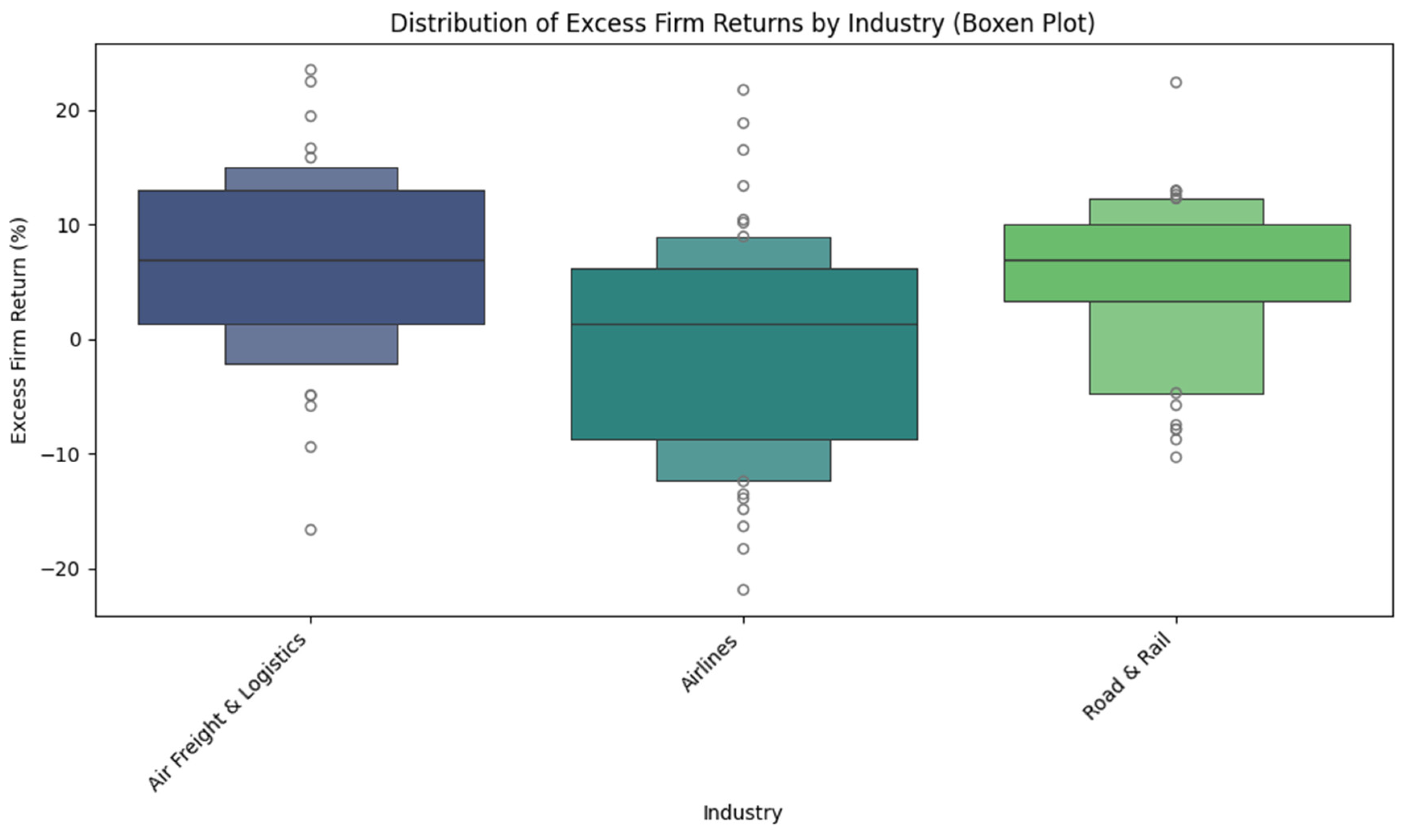
Figure 2.
Mean ESG by Year with Standard Deviation.
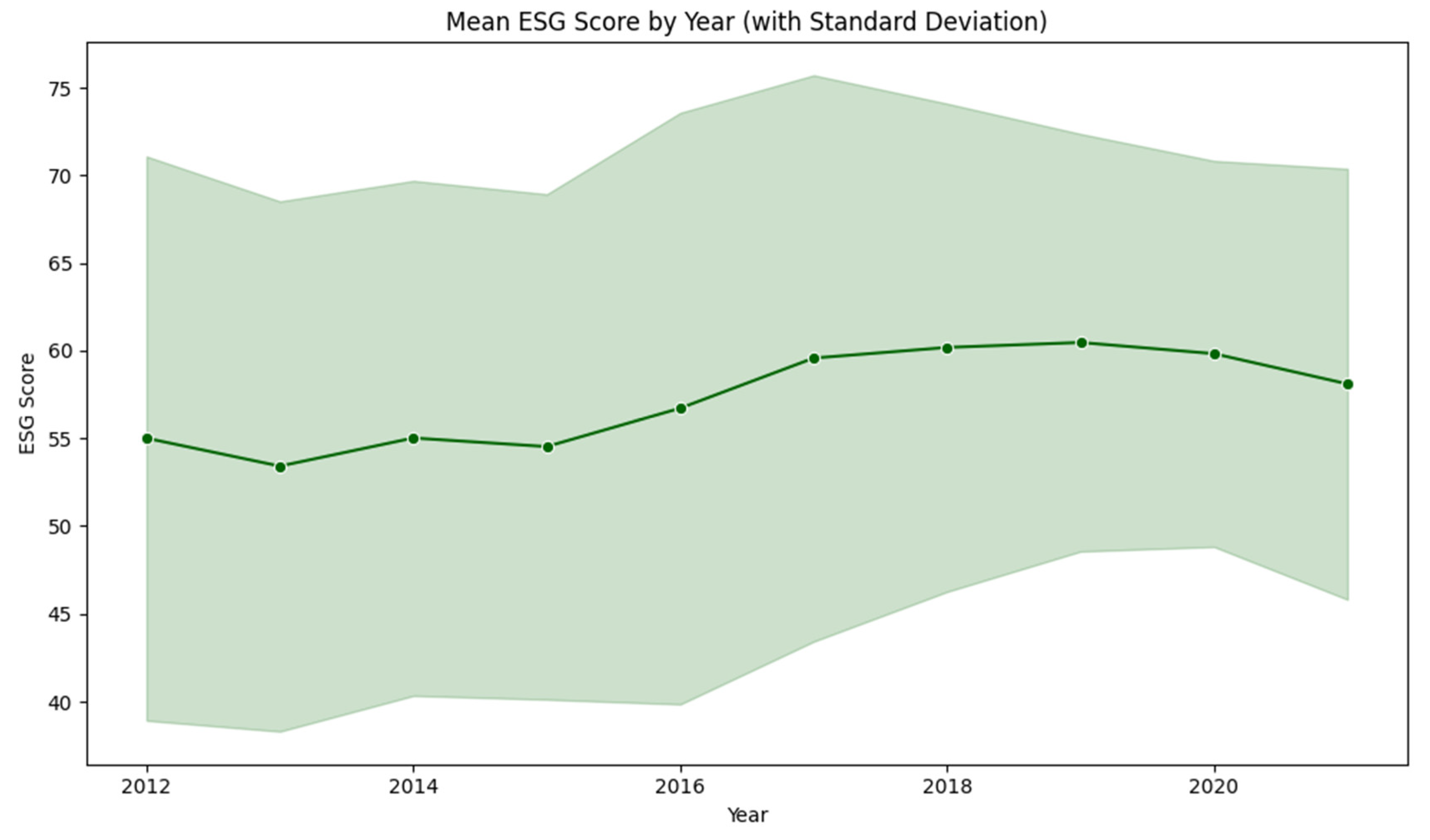
Figure 3.
ROC AUC Curves for Random Forest and XGBoost.
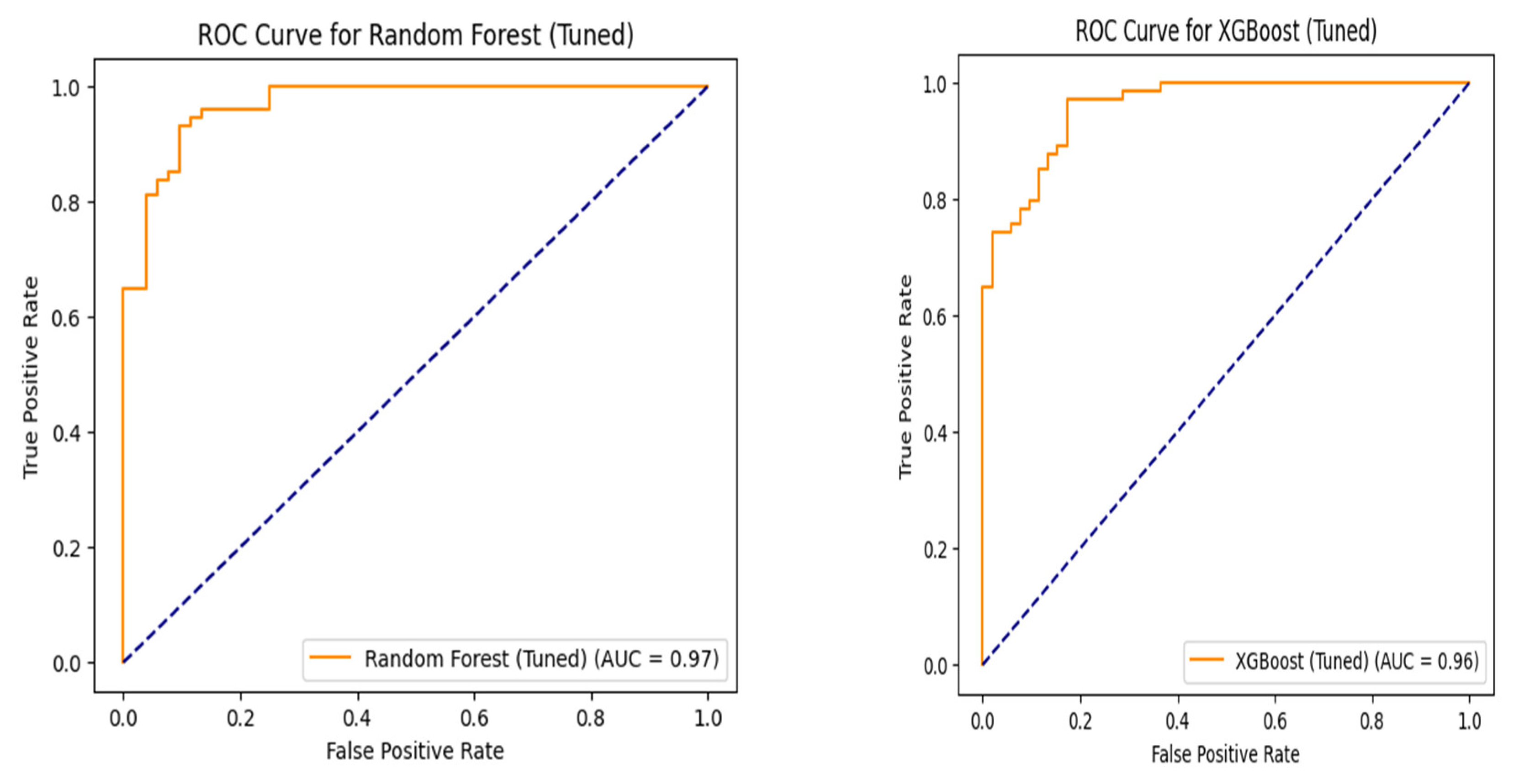
Figure 4.
Top 10 Feature Importances (Random Forest).
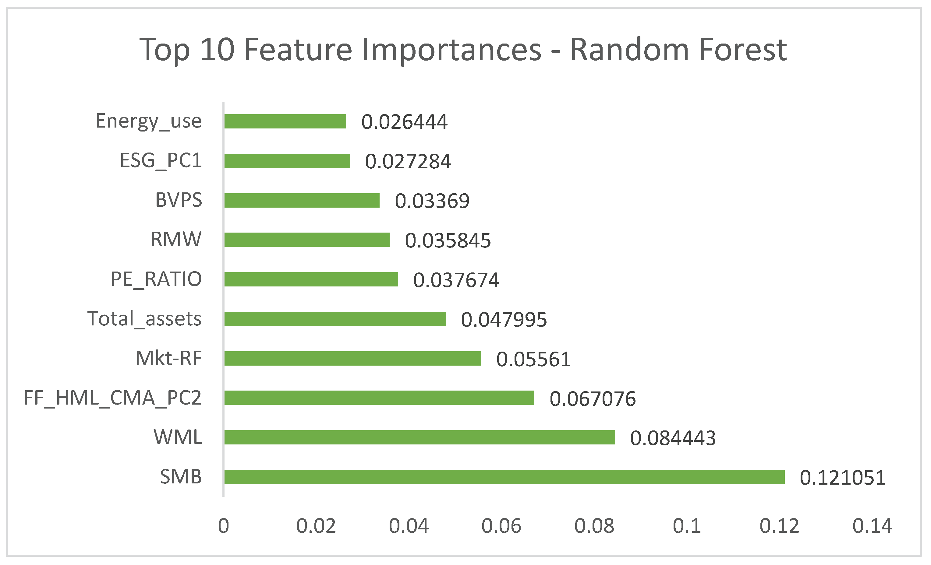
Figure 5.
Top 10 Feature Importances (XGBoost).
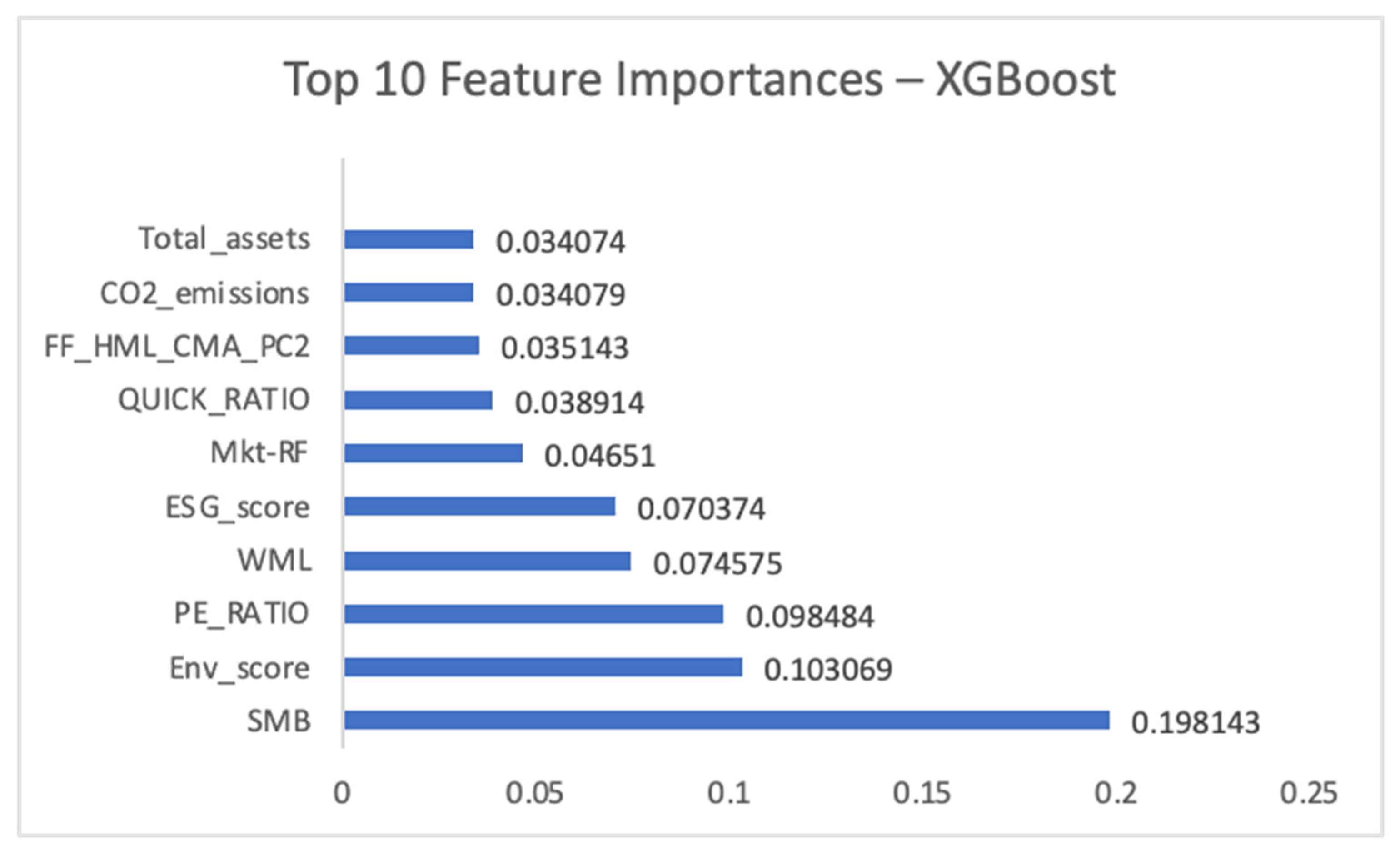
Figure 6.
SHAP Summary Plot (Random Forest).
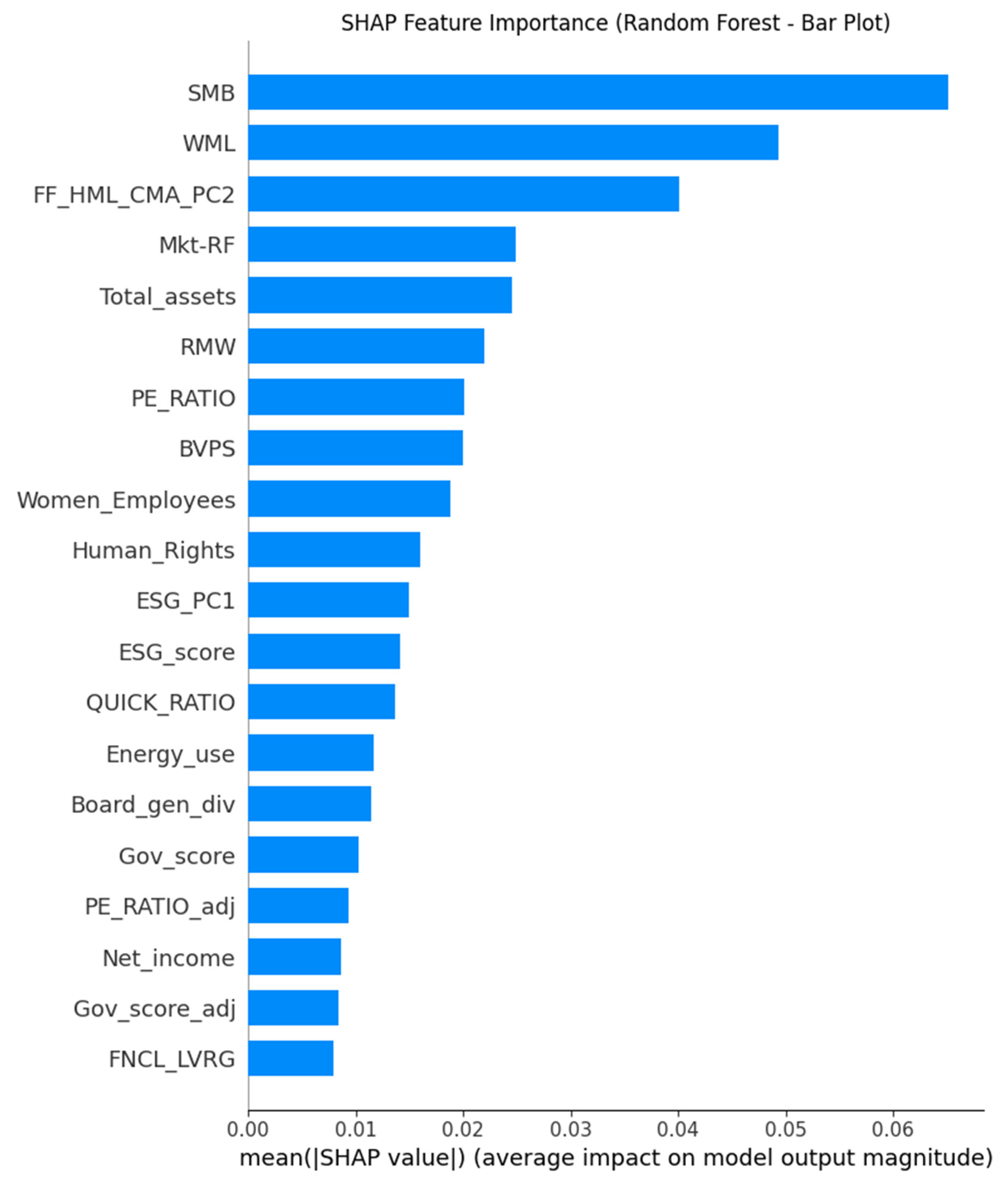
Figure 7.
SHAP Dependence Plots (Random Forest).
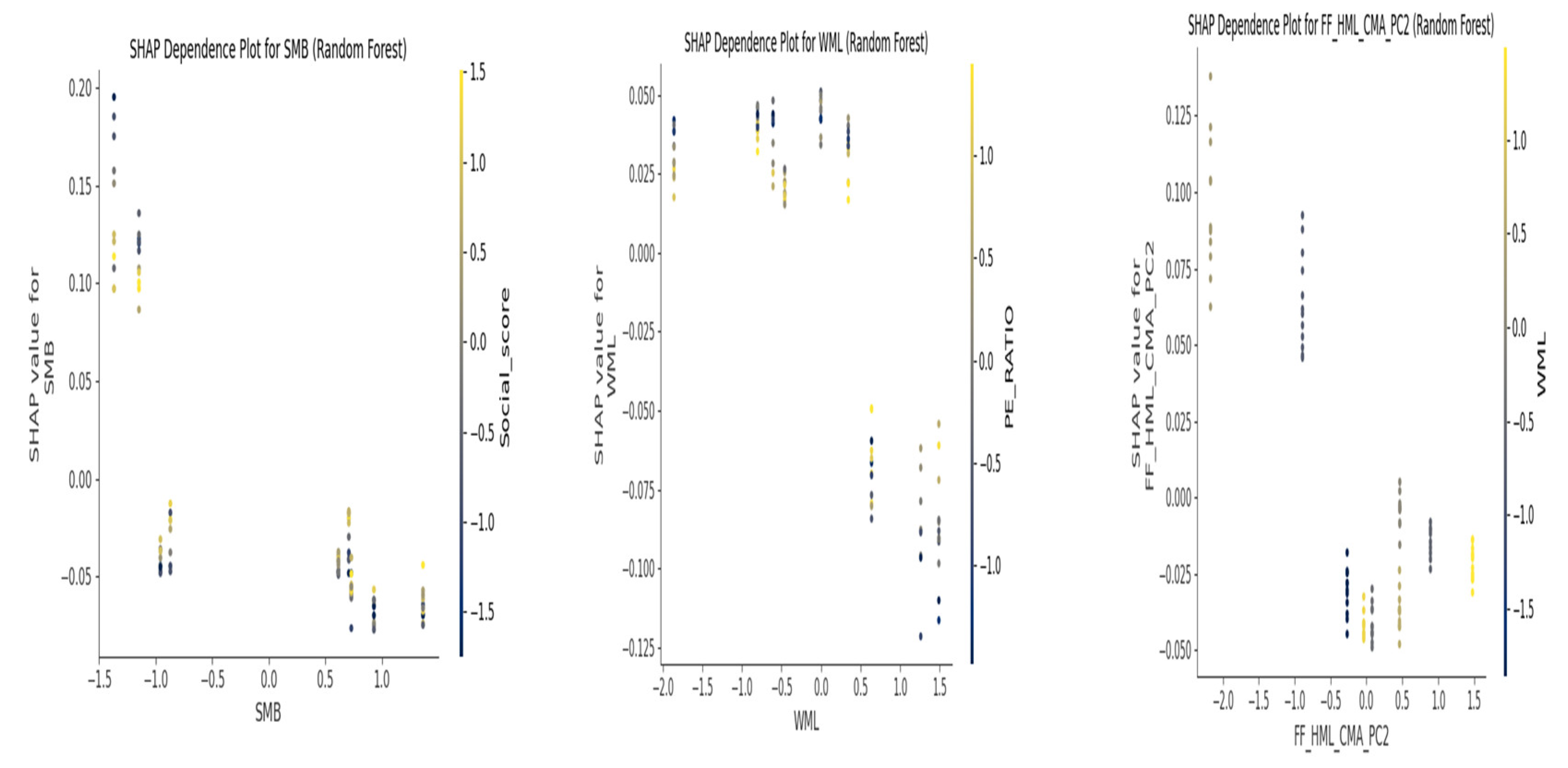
Figure 8.
SHAP Summary Plot (XGBoost).
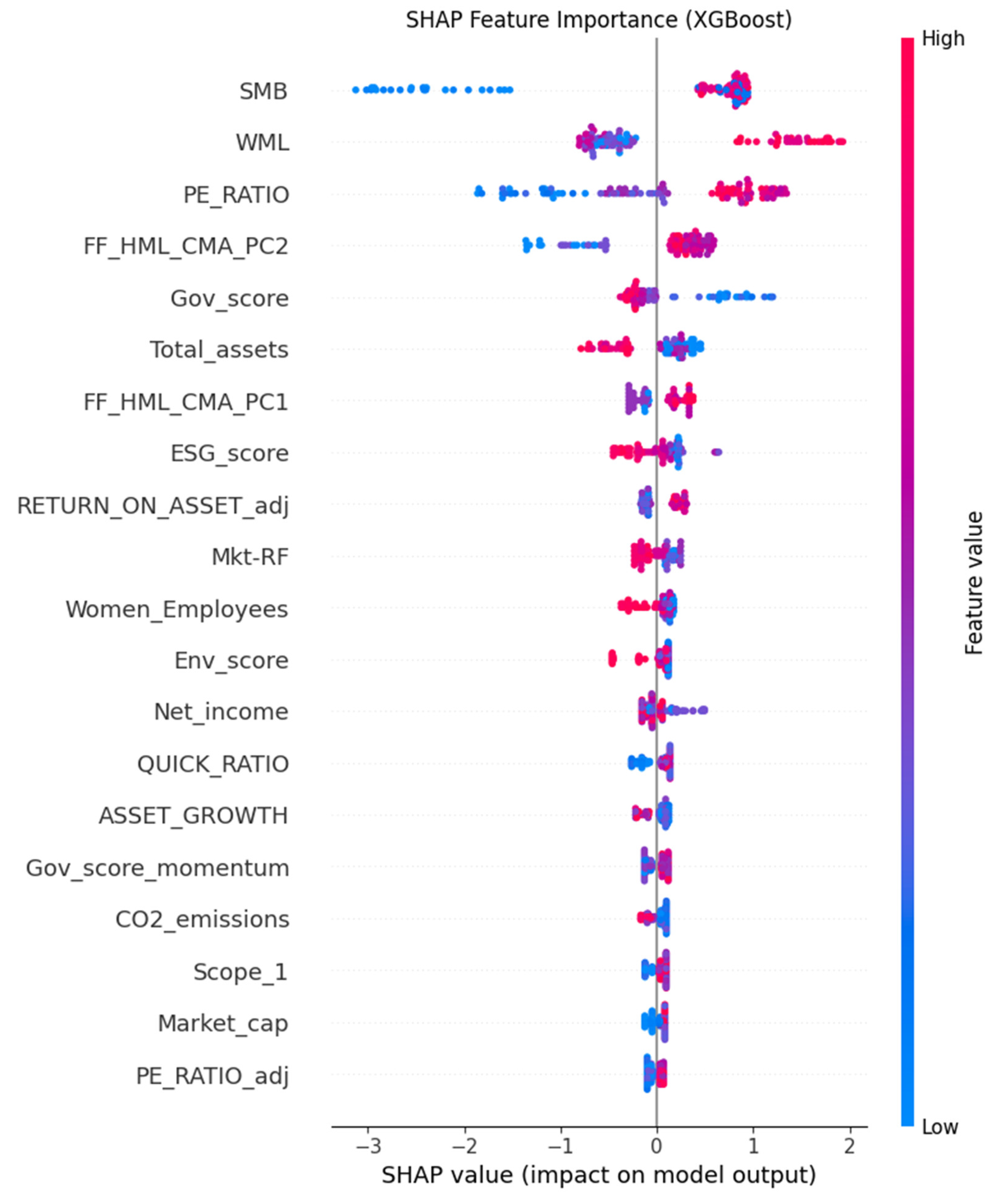
Figure 9.
SHAP Dependence Plots (XGBoost).
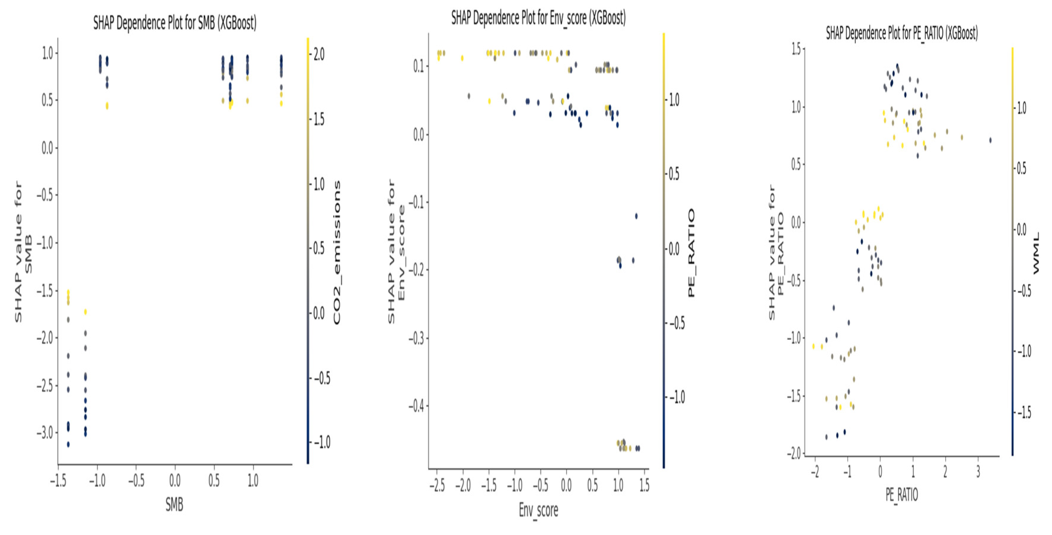

Table 1.
PCA Explained Variance for ESG and Asset Pricing Factors (HML, CMA).
| Component | Explained Variance Ratio | Cumulative Explained Variance |
| ESG_PC1 | 0.7143 | 0.7143 |
| FF_HML_CMA_PC1 | 0.9907 | 0.9907 |
| FF_HML_CMA_PC2 | 0.0093 | 1.0000 |
Table 2.
VIF Check for Multicollinearity.
| Feature | VIF |
| Const | - |
| Mkt-RF | 1.210768 |
| SMB | 2.085959 |
| RMW | 2.706104 |
| WML | 1.701949 |
| FF_HML_CMA_PC1 | 1.764844 |
| FF_HML_CMA_PC2 | 1.959887 |
| ESG_score | 1.024254 |
Table 3.
Panel Regression Results for Excess Firm Returns (Robust Standard Errors).
| Variable | Pooled OLS (Robust) | Std. Err. | T-stat | P-value | FE (Robust) | Std. Err. (FE) | T-stat (FE) | P-value (FE) | RE (Robust) | Std. Err. (RE) | T-stat (RE) | P-value (RE) |
| const | 14.66 | 2.49 | 5.88 | 0 | 9.17 | 4.34 | 2.11 | 0.04 | 11.1 | 4.05 | 2.74 | 0.01 |
| Mkt-RF | -0.12 | 0.04 | -3.06 | 0 | -0.13 | 0.04 | -2.89 | 0 | -0.12 | 0.04 | -3.22 | 0 |
| SMB | 0.59 | 0.17 | 3.58 | 0 | 0.61 | 0.18 | 3.46 | 0 | 0.61 | 0.16 | 3.79 | 0 |
| RMW | 0.41 | 0.25 | 1.65 | 0.1 | 0.41 | 0.22 | 1.92 | 0.06 | 0.41 | 0.21 | 1.96 | 0.05 |
| WML | 0.46 | 0.08 | 5.61 | 0 | 0.48 | 0.08 | 6.2 | 0 | 0.47 | 0.07 | 6.49 | 0 |
| FF_HML_CMA_PC1 | 4.15 | 0.66 | 6.28 | 0 | 4.3 | 0.53 | 8.1 | 0 | 4.25 | 0.55 | 7.71 | 0 |
| FF_HML_CMA_PC2 | -11.56 | 4.83 | -2.39 | 0.02 | -11.05 | 4.16 | -2.65 | 0.01 | -11.23 | 3.99 | -2.82 | 0.01 |
| ESG_score | -0.22 | 0.04 | -5.76 | 0 | -0.12 | 0.07 | -1.73 | 0.09 | -0.16 | 0.06 | -2.62 | 0.01 |
| Model Summary | Pooled OLS | Fixed Effects | Random Effects | |||||||||
| R-squared (Within) | 0.52 | 0.53 | 0.53 | |||||||||
| R-squared (Between) | 0.42 | 0.32 | 0.37 | |||||||||
| R-squared (Overall) | 0.5 | 0.48 | 0.49 | |||||||||
| No. Observations | 140 | 140 | 140 | |||||||||
| No. Entities | 14 | 14 | 14 | |||||||||
| No. Time periods | 10 | 10 | 10 | |||||||||
| F-statistic | 26.57 | 18.69 | 22.37 | |||||||||
| P-value | 0 | 0 | 0 | |||||||||
Table 4.
Panel Model Selection Tests.
| Test | Statistic | P-value | Conclusion |
| F-test for Poolability | 3.904 | 0 | Fixed Effects preferred over Pooled OLS (entity effects are significant) |
| Hausman Test (FE vs RE) | Not available | - | Fixed Effects is significant overall |
Table 5.
Panel Regression Results with Decomposed ESG Factors (Robust Standard Errors).
| Parameter | Coefficient | Std. Err. | T-stat | P-value | Lower CI | Upper CI |
| Const | 1005.8 | 932.16 | 1.08 | 0.28 | -840.1 | 2851.8 |
| Mkt-RF | -0.03 | 0.06 | -0.52 | 0.6 | -0.14 | 0.08 |
| SMB | 0.59 | 0.17 | 3.42 | 0 | 0.25 | 0.94 |
| RMW | 0.08 | 0.22 | 0.37 | 0.71 | -0.36 | 0.52 |
| WML | 0.01 | 0.07 | 0.07 | 0.94 | -0.14 | 0.15 |
| ESG_PC1 | 139.37 | 131.77 | 1.06 | 0.29 | -121.57 | 400.31 |
| Social_score | -7.7 | 7.09 | -1.09 | 0.28 | -21.74 | 6.33 |
| Gov_score | -4.44 | 4.11 | -1.08 | 0.28 | -12.59 | 3.7 |
| Env_score | -5.28 | 5.04 | -1.05 | 0.3 | -15.26 | 4.69 |
| Model Summary | PanelOLS | |||||
| Dep. Variable | Excess_Return_Firm | |||||
| R-squared (Within) | 0.1821 | |||||
| R-squared (Between) | 0.1026 | |||||
| R-squared (Overall) | 0.1622 | |||||
| No. Observations | 140 | |||||
| F-statistic (robust) | 4.2458 | |||||
| P-value | 0.0002 | |||||
Table 6.
ADF Test Results for Stationarity.
| Variable | Test Type | ADF Statistic | P-value | Critical Values (1%, 5%, 10%) | Conclusion |
| Mkt-RF | Levels | -3.53 | 0.0073 | {1%: -4.47, 5%: -3.29, 10%: -2.77} | Likely Stationary (I(0)) |
| Market_ESG_Factor_VW | Levels | -1.97 | 0.2979 | {1%: -4.47, 5%: -3.29, 10%: -2.77} | Likely Non-Stationary (I(1) or higher) |
| Market_ESG_Factor_VW_diff | First Difference | -3.06 | 0.0293 | {1%: -5.35, 5%: -3.65, 10%: -2.90} | Likely Stationary (I(1)) |
Table 7.
VAR Model Estimation Summary.
| Model Summary | Value | |||
| Model | VAR | |||
| Method | OLS | |||
| No. of Equations | 2 | |||
| Nobs | 9 | |||
| Log likelihood | -14.627 | |||
| AIC | -1.98085 | |||
| BIC | -1.93703 | |||
| HQIC | -2.07543 | |||
| FPE | 0.138206 | |||
| Det(Omega_mle) | 0.111947 | |||
| Equation: Mkt-RF | Coefficient | Std. Error | T-stat | P-value |
| Const | 0.124225 | 0.044253 | 2.807 | 0.005 |
| Equation: Market_ESG_Factor_VW_diff | Coefficient | Std. Error | T-stat | P-value |
| Const | 0.045688 | 0.842179 | 0.054 | 0.957 |
| Correlation Matrix of Residuals | Mkt-RF | Market_ESG_Factor_VW_diff | ||
| Mkt-RF | 1 | -0.070412 | ||
| Market_ESG_Factor_VW_diff | -0.07041 | 1 | ||
Table 8.
Granger Causality Test Results.
| Hypothesis | Lag | P-value | Conclusion |
| Mkt-RF Granger-causes Market_ESG_Factor_VW | 1 | 0.4441 | No strong evidence of Granger causality |
| Mkt-RF Granger-causes Market_ESG_Factor_VW | 2 | 0.8987 | No strong evidence of Granger causality |
| Market_ESG_Factor_VW Granger-causes Mkt-RF | 1 | 0.7675 | No strong evidence of Granger causality |
| Market_ESG_Factor_VW Granger-causes Mkt-RF | 2 | 0.8062 | No strong evidence of Granger causality |
Table 9.
GARCH(1,1) Model Results for Market Excess Returns Volatility.
| Mean Model | ||||||
| Parameter | Coefficient | Std. Err. | T-stat | P>|t| | 95% CI Lower | 95% CI Upper |
| Mu | 0.1289 | 0.03835 | 3.36 | 0.00078 | 0.0537 | 0.204 |
| Volatility Model | ||||||
| Parameter | Coefficient | Std. Err. | T-stat | P>|t| | 95% CI Lower | 95% CI Upper |
| Omega | 0.004683 | 0.01018 | 0.46 | 0.645 | -0.015 | 0.02464 |
| alpha [1] | 6.74E-16 | 0.01911 | 3.52E-14 | 1 | -0.037 | 0.03746 |
| beta[1] | 0.6866 | 0.796 | 0.863 | 0.388 | -0.873 | 2.247 |
| Model Summary | Value | |||||
| Dep. Variable | Mkt-RF | |||||
| R-squared | 0 | |||||
| Adj. R-squared | 0 | |||||
| Log-Likelihood | 7.06041 | |||||
| AIC | -6.12082 | |||||
| BIC | -4.91048 | |||||
| No. Observations | 10 | |||||
| Df Residuals | 9 | |||||
| Df Model | 1 | |||||
| Covariance Estimator | Robust | |||||
Table 10.
Hyperparameter Tuning Results (Random Forest and XGBoost).
| Model | Best Parameters | Best ROC AUC (CV) |
| Random Forest | {‘max_depth’: 5, ‘min_samples_split’: 5, ‘n_estimators’: 50} | 0.982 |
| XGBoost | {‘eval_metric’: ‘logloss’, ‘learning_rate’: 0.1, ‘max_depth’: 3, ‘n_estimators’: 100, ‘use_label_encoder’: False} | 0.9716 |
Table 11.
Consolidated Cross-Validation Performance Metrics.
| Performance Metrics | ||||
| Metric (Aggregated CV) | Random Forest | XGBoost | ||
| Accuracy | 0.9206 | 0.8651 | ||
| Precision | 0.9103 | 0.8904 | ||
| Recall | 0.9595 | 0.8784 | ||
| F1-Score | 0.9342 | 0.8844 | ||
| ROC AUC | 0.9699 | 0.9592 | ||
| Classification Report (Random Forest) | ||||
| Class | Precision | Recall | F1-Score | Support |
| Class 0 | 0.94 | 0.87 | 0.9 | 52 |
| Class 1 | 0.91 | 0.96 | 0.93 | 74 |
| Accuracy | 0.92 | 126 | ||
| Macro Avg | 0.92 | 0.91 | 0.92 | 126 |
| Weighted Avg | 0.92 | 0.92 | 0.92 | 126 |
| Classification Report (XGBoost) | ||||
| Class | Precision | Recall | F1-Score | Support |
| Class 0 | 0.83 | 0.85 | 0.84 | 52 |
| Class 1 | 0.89 | 0.88 | 0.88 | 74 |
| Accuracy | 0.87 | 126 | ||
| Macro Avg | 0.86 | 0.86 | 0.86 | 126 |
| Weighted Avg | 0.87 | 0.87 | 0.87 | 126 |
Disclaimer/Publisher’s Note: The statements, opinions and data contained in all publications are solely those of the individual author(s) and contributor(s) and not of MDPI and/or the editor(s). MDPI and/or the editor(s) disclaim responsibility for any injury to people or property resulting from any ideas, methods, instructions or products referred to in the content. |
© 2025 by the authors. Licensee MDPI, Basel, Switzerland. This article is an open access article distributed under the terms and conditions of the Creative Commons Attribution (CC BY) license (http://creativecommons.org/licenses/by/4.0/).
Copyright: This open access article is published under a Creative Commons CC BY 4.0 license, which permit the free download, distribution, and reuse, provided that the author and preprint are cited in any reuse.


