

Submitted:
08 June 2025
Posted:
09 June 2025
You are already at the latest version
Abstract
With the large-scale construction and operation of urban underground utility tunnels in China, the associated safety issues cannot be ignored. This paper proposes a risk assessment method for cable duct fires by optimizing the Bayesian model and combining bidirectional inference and decision support to numerically analyze the impact of different ventilation and fire protection measures on fires, and evaluate risk levels using the risk matrix method. During forward and diagnostic reasoning analysis, the predicted probability of a cable duct fire occurring is 4.967‰, and the probabilities of the cable duct fire developing to various stages are 3.533‰, 1.378‰ and 1.232‰, respectively. Bayesian network-assisted decision analysis yields the maximum causation chain for cable duct fires as: insulation damage (X6) → poor connection (D1) → leakage (C2) → cable core overheating (B1) → cable self-ignition (A1) → cable ignition (T). Then, through Bayesian network probability self-adaptive analysis, the probability of cable duct fire occurrence and the probabilities of various consequence scenarios increase over time, with the upward trend reflecting the deteriorating operating conditions of the cable duct. Finally, based on the dynamic Bayesian model and inference, the predicted probability of cable ignition increases from 4.967‰ at T0 to 14.69‰ at T29.
Keywords:
utility tunnel
; cable duct
; dynamic Bayesian network
; reliability
1. Introduction
With the continuous development of society and the gradual acceleration of urbani.
zation, people’s demand for municipal infrastructure such as gas, electricity, communications, and water supply has been increasing. Therefore, the effective utilization of underground space has received increasing attention from scholars. The urban underground utility tunnel is a comprehensive system integrating power, telecommunications, natural gas, water supply, and other municipal cables, pipelines, and monitoring equipment. The earliest utility tunnel appeared in France in 1833 to address urban water supply and sewage system issues. Subsequently, many developed countries such as the United States and Russia began planning the construction of utility tunnels [1,2,3].
The development of fire risk assessment methods and techniques has played a driving role in the progress of fire science [4]. At the same time, conducting fire risk assessments has guiding significance for fire risk control, performance-based fire protection technology, and fire service operations. Domestic and foreign scholars have proposed many methods for fire risk assessment, which can be broadly classified into qualitative, quantitative, and semi-quantitative analysis methods based on the nature of the research methods [5]. Qualitative fire risk assessment methods refer to describing, analyzing, and identifying fires in a non-quantified form [6,7].
Common qualitative fire risk analysis methods include safety checklist methods, fault tree analysis, HAZOP, and others. In this area of research, Quanle [8] proposed a fire risk assessment method based on safety checklists for large and medium-sized urban shopping malls and verified the applicability of the method using Walmart as an example. Xie [9] proposed a new BT model quantitative risk assessment algorithm combining fuzzy cloud membership functions with cloud analytic hierarchy process and probability estimation. The proposed method was applied to a case study of an oil depot in Dalian, and the results showed that it could accurately identify the weaknesses of the oil depot system. Aihua [10] proposed a dynamic risk assessment model for gas pipelines based on system dynamics, considering the time-varying nature of the system. Through case analysis, it was shown that this model could characterize the dynamic variation of gas pipeline risk over time. Wang [11] constructed an uncertain dynamic Bayesian network model for dual-gradient drilling systems, predicting the dynamic occurrence probabilities of various risk events in the drilling system, and validated the model using Petri nets. Ming [12] combined dynamic bowtie analysis and DBN for dynamic risk assessment of heating furnaces in petrochemical enterprises. In the study of fire smoke, Liu et al. [13] investigated the temperature distribution characteristics of enclosed utility tunnels through small-scale fire experiments, concluding that the vertical temperature distribution in utility tunnel fires has a distinct stratification, and the temperature of fire smoke in the enclosed space cannot be ignored.
As an intensive and efficient urban infrastructure, the urban underground utility tunnel has become an important component of modern urban construction. However, with the increasing functions and complexity of utility tunnels, safety issues have become increasingly prominent, particularly the assessment and management of cable vault fire risks [14,15,16]. Traditional risk assessment methods often fail to accurately reflect the dynamic changes in fire risk, and researchers have begun seeking more advanced technical means to address this challenge. Dynamic fire risk assessment of urban underground utility tunnel cable vaults based on dynamic Bayesian networks is an emerging and promising research area [17,18,19]. Although there are still certain challenges and problems, with continuous technological advancements and in-depth research, it is believed that DBNs will play an increasingly important role in cable vault fire risk assessment in the future, providing more scientific and accurate technical support for the safe operation of urban underground utility tunnels [20,21].
Currently, there are some deficiencies in the research on fire risk assessment of urban underground utility tunnel cable vaults. Although semi-quantitative risk analysis methods have been widely applied in fire accident studies, quantitative risk assessment methods based on the dual nature of fires have not been sufficiently studied. To address the shortcomings in dynamic risk assessment of utility tunnel cable vault fires, this paper combines Bayesian methods to analyze and predict cable vault fire probabilities and employs numerical simulations and risk matrices to comprehensively assess the dynamic risk levels of cable vault fires.
2. Methods
2.1. Bayesian Networks
Bayesian network (BN) inference is a probabilistic reasoning method based on Bayes’ theorem, which assists analysis and decision-making through three approaches: forward inference, backward inference, and decision support inference. Forward inference calculates the probability of the target node from the known root node probabilities and conditional probabilities; backward inference starts from the probability of the target node and infers the probability of the root node, commonly used for diagnostic reasoning; decision support inference identifies the key factors and paths influencing the target event through sensitivity and impact analysis, providing decision support.
A dynamic Bayesian network (DBN) is a special Bayesian model that combines a Markov chain model. Not only can DBNs handle uncertain relationships of the research object, but they can also process time-series data. Furthermore, dynamic Bayesian networks consider the time factor, i.e., knowledge accumulation, and perform probabilistic prediction and other inferences through information accumulated over time. Dynamic Bayesian networks are an extension of Bayesian networks that consider the probability of an event occurring over the time dimension.
2.2. Construction of Dynamic Bayesian Networks
Based on the initial Bayesian model, constructing a dynamic Bayesian model also requires extending the initial Bayesian network over a timeline. Using software like Genie to build a DBN model, first determine the dynamic nodes of the dynamic Bayesian network, then connect the nodes themselves with arcs, and set the time-lag influence relationships. Finally, determine the transition probability distribution of the dynamic Bayesian network.
Similar to Bayesian inference, dynamic Bayesian theory also has three inference approaches: forward inference, backward inference, and decision support inference. However, dynamic Bayesian networks can additionally calculate the probability values for each time slice. Forward inference in a DBN model refers to predicting the probability of the top event occurring in each time slice after setting the prior probabilities, conditional probabilities, transition probability distributions, and time lags. Backward inference in dynamic Bayesian networks similarly sets the event occurrence probability or fuzzy state and infers the basic event with the maximum posterior probability.
2.3. Fire Smoke Movement Model
In fire consequence simulation, various fire smoke movement models have emerged, such as zone models represented by CFAST, field models represented by FDS, network models, and field-zone network models. Among these, zone models and field models are the most widely applied. The CFAST model divides the tunnel into two zones, upper and lower, and is not suitable for long, narrow tunnels, nor does it provide high enough simulation accuracy. Field simulation, on the other hand, averagely divides the entire area into numerous small cells, using the basic equations for each cell, resulting in higher computational accuracy. Additionally, adjacent cells are balanced. Due to the narrow, enclosed characteristics of urban underground utility tunnels, numerical simulation software based on field simulation is suitable for simulating the consequences of cable duct fires.
The large eddy simulation (LES) method involves filtering the viscous fluid equations and then dividing the flow into large and small-scale quantities. The large-scale quantities can be directly simulated, while the small-scale quantities require a subgrid model for correction, greatly reducing the computational load. Therefore, this paper adopts the large eddy simulation method for simulating the fire consequences in cable ducts of urban underground utility tunnels.
There are two models for describing fire development in FDS software: a finite reaction rate model and a mixture fraction model. The mixture fraction model is more widely applied and suitable for large eddy simulation; thus, this paper uses the mixture fraction model for simulating cable ducts in utility tunnels.
2.4. Cable Duct Fire Risk Matrix
The risk matrix method is a comprehensive approach for risk identification and risk assessment in system risk analysis. The possibility of a hazardous event occurring, i.e., the probability of a cable duct fire scenario, can be graded based on actual conditions and the probability intervals recommended by the International Tunnelling Association, as shown in Table 2.1.
The severity of a hazardous event refers to the severity of the consequences of a cable duct fire scenario. According to the characteristics of cable duct fire scenarios, Consequence Stage III represents the failure of fire brigades to extinguish the fire, which is of little significance for consequence analysis; Consequence Stage II represents the failure of the sprinkler system, contingent on the occurrence of Stage I (failure of personnel to extinguish the fire). Therefore, the typical Stage I condition is selected for consequence simulation and analysis.
The assessment of the severity of fire consequences in utility tunnel cable ducts mainly considers the degree of damage to the tunnel structure and the degree of damage to materials within the cable duct. For the tunnel structure, utility tunnels are constructed from cast concrete, and concrete loses strength significantly after 300°C and rapidly deteriorates with minimal performance recovery above 400°C. Within the cable duct, the main materials are PVC cable jackets and electronic equipment; according to research by the U.S. Nuclear Regulatory Commission, the critical failure temperature for thermoplastic PVC cables is approximately 200°C, and electronic equipment generally starts to sustain damage at 150°C. Based on the above, the severity level standards for fire consequences in utility tunnel cable ducts are established, as shown in Table 2.2.
To assess the overall risk level of cable duct fires by considering both the possibility and severity, a risk matrix is proposed to grade the risk levels of cable fire scenarios. Based on the risk matrix and engineering practice, a risk matrix for the possibility and severity of consequences of utility tunnel cable duct fires is established, as shown in Table 2.3. Table 2.4 presents the risk level classification standards for the utility tunnel cable duct fire risk matrix.
3. Results and Discussions
3.1. Cable Room Fire Risk Analysis Based on Bayesian Network
In the parameter learning of BN, assuming two parent nodes X1 and X2 have Y and N states respectively, and the child node T also has Y and N states. Typically, when the state of the child node is closer to the state of the parent node, the probability of the parent node causing the child event to occur will increase significantly. Therefore, this paper can complete the calculation of the conditional probability of non-root nodes through the following steps: node state assignment, determination of the fuzzy judgment matrix, determination of the initial weight, defuzzification, calculation of all node states, and finally calculation of the child node conditional probability according to equation (3.1).
In the equation, R is the result distribution exponent. The larger the R value, the more similar the states of the parent node and the child node are. The R value is typically determined by expert judgment. Taking the cable overload node in the cable fire accident model as an example, cable overload is caused by circuit breaker failure, overvoltage, and stray current. First, based on the rich experience and professional knowledge of three experts, the judgment matrix shown in Table 3.1 is established, and then the expert judgments are aggregated to obtain Table 3.2.
By calculation, the conditional probability table of cable overload is obtained as shown in Table 3.3. There are two states for each circuit breaker failure, overvoltage, and stray current that cause cable overload, giving a total of 8 state combinations. When circuit breaker failure, overvoltage, and stray current occur simultaneously, the probability of cable overload is the highest, reaching around 73%. Conversely, when the circuit breaker is functioning normally, the voltage is within the normal range, and there is no stray current, the probability of cable overload is extremely low. This shows that the network parameters of the model constructed in this paper can match the actual situation well.
3.2. Cable Fire Probability Prediction and Fault Diagnosis Based on Bayesian Network
Unlike the bow-tie method, the Bayesian network is a method for probabilistic reasoning and prediction, overcoming the static limitations of the bow-tie method, and can also realize forward and backward linear prediction and diagnostic analysis. In probability prediction analysis, according to the prior probability of the root nodes and their conditional dependencies, the probability of cable fire occurrence can be calculated as 4.967‰. The prior probabilities of the root nodes come from estimates of the probabilities appearing in the literature and historical data or comprehensive expert evaluation, as shown in Table 3.4, and the reliability of various safety barriers are shown in Table 3.5. From the BN model inference, the probability of cable room fire reaching stage I can also be obtained as 3.533‰; the probability of fire development to stage II is 1.378‰, and the probability of developing to stage III is 1.232‰. The order of probability magnitude is stage I > stage II > stage III. This is consistent with the actual logic, verifying the feasibility of the model. The reasoning results show that after a cable room fire occurs, the consequence scenario of stage I has the highest probability of occurrence because both stage II and stage III are premised on the occurrence of stage I.
Bayesian backward inference is commonly used for fault diagnosis. In the model, the most likely basic events can be inferred by setting the occurrence probability or state of the top event. In the BN model constructed in this paper, by setting the occurrence probability of the top event of cable fire to 100%, i.e., assuming the cable fire occurs, the occurrence probabilities of the root nodes are inferred backward. The posterior probability distributions of the various root nodes are obtained as shown in Table 3.4.
3.3. Maximum Causal Chain Analysis Based on Bayesian Network
For diagnostic reasoning based on the Bayesian network, the Bayesian network-assisted decision reasoning can be used for further risk analysis of cable fire accidents. The maximum causal chain analysis, also known as influence strength analysis, can analyze the strength of influences between nodes layer by layer, which is expressed by the thickness of the connecting arcs in the model. After performing diagnostic reasoning on the cable fire Bayesian network model, by selecting “Influence Strength” analysis in the Genie software, the causal chains and the maximum causal chain of cable fires can be analyzed.
In the cable fire BN model, the maximum causal chain is: Insulation damage (X6) → Poor connection (D1) → Leakage (C2) → Cable core overheating (B1) → Cable self-ignition (A1) → Cable fire (T).
The process is as follows:
(1) Between the two parent nodes of T (Cable fire), A1 (Cable self-ignition) and A2 (External fire source), A1 has a higher posterior probability, resulting in the chain (A1 → T).
(2) Between the two parent nodes of A1, B1 (Cable core overheating) and B2 (Arcing fault), B1 has the highest posterior probability, resulting in the chain (B1 → A1 → T).
(3) Among the three parent nodes of B1, C1 (Poor heat dissipation), C2 (Leakage), and C3 (Cable short circuit), C2 has the highest posterior probability, resulting in the chain (C2 → B1 → A1 → T).
(4) Between the two parent nodes of C2, D1 (Poor connection) and D2 (Cable overload), D1 has the highest posterior probability, resulting in the chain (D1 → C2 → B1 → A1 → T).
(5) Among the three parent nodes of D1, X4 (Terminal corrosion), X5 (Poor installation quality), and X6 (Insulation damage), X6 has the highest posterior probability, resulting in the chain (X6 → D1 → C2 → B1 → A1 → T).
Through the analysis, the maximum causal chain leading to the cable trunk fire is (X6 → D1 → C2 → B1 → A1 → T). Of course, this is only the most likely causal chain, and there are many other causal chains, such as (X3 → C1 → B1 → A1 → T), (X9 → C4 → C2 → B1 → A1 → T), and (X23 → A2 → T). In terms of probability of occurrence, they are not the maximum causal chains leading to the cable trunk fire, but the randomness of fire determines that any causal chain has a possibility of occurrence.
By obtaining the maximum causal chain of the cable trunk fire, the most efficient safety monitoring chain for the system is obtained. In other words, if safety monitoring and management measures are formulated for cable trunk fire accidents, the safety monitoring work on insulation damage, cable overload, leakage, cable core overheating, and cable self-ignition can be prioritized as the first stage.
3.4. Cable Trunk Fire Risk Analysis Based on DBN
After constructing the initial Bayesian network for cable fires, a dynamic Bayesian network needs to be further constructed by considering the time-varying nature of the factors. However, it is difficult to consider the time-varying nature of each node in the initial cable fire Bayesian network. Calculating the state transition matrix in the dynamic Bayesian network would be a complex task. Moreover, not all nodes in the initial Bayesian network have a significant degree of time variation. Therefore, the risk factors of cable fires with high time variability can be selected as dynamic nodes for the dynamic Bayesian network.
Referring to the classification of basic factors for gas pipelines by the American PRCI, the risk factors of cable accidents are divided into dynamic and static risk factors, as shown in Table 3.6.
Additionally, constructing a DBN model requires defining the transition network probability tables. The transition probability distribution can generally be obtained through expert experience or training from sample data. The transition probability distribution is an important parameter that expresses the ability of the dynamic Bayesian network to perform dynamic reasoning analysis using actual monitoring data. Based on the three assumptions of DBN and expert knowledge, the transition network probability table shown in Table 3.7 is obtained.
After defining the initial Bayesian network model for cable fires, the dynamic Bayesian network model can be constructed using the GeNIe software tool, as shown in Figure 3.1.
3.5. Cable Fire Probability Prediction Based on Dynamic Bayesian Network
According to the dynamic Bayesian model for cable fires established in this paper, forward inference is performed to predict the probability of cable trunk fires in utility tunnels. In the GeNIe software, the “SetEvidence” function is used to input the initial state of the nodes. Additionally, the prediction range and step size need to be set. After setting the state of each node, to predict the probability change of cable fires over the next 30 years, the prediction range is set to 30 time slices, with an interval of 1 year between any two time slices. The probability table of the entire network model is updated, and the probability table of the top event occurring in each time slice is obtained.
Fault diagnosis is a method of backward reasoning, where the state of the top event occurring is set, and the posterior probabilities of the root nodes are inferred backward to determine the influence of the root nodes on the occurrence of the top event. In addition to inferring the posterior probabilities of the root nodes, fault diagnosis analysis in dynamic Bayesian networks can also obtain the posterior probability distribution of the root nodes at different time slices. With the prediction range set to 10 time slices, the posterior probabilities of each node at the T9 moment are shown in Table 3.8.
At the T9 moment, among the basic events causing cable fires, the probability value of the State1 status of the node variable insulation aging is the largest at 875.5‰, which requires attention during routine utility tunnel maintenance. Next, the probability values of the node variables long-term overload and dielectric strength reduction being in State1 at the T9 moment are 323.0‰ and 259.1‰, respectively, which are significantly higher than other nodes.
In this paper, ten time slices were set, and the dynamic Bayesian network diagnostic reasoning also obtained the posterior probability distribution of each node at different time slices. Table 3.9 and Table 3.10 show the posterior probability distributions of the root nodes’ terminal corrosion and stray current at different moments. The posterior probability distributions of the remaining root nodes at different time slices can also be obtained.

Table 3.9.
Posterior Probabilities of Terminal Corrosion at Different Moments.
| Moment | T0 | T1 | T2 | T3 | T4 | T5 | T6 | T7 | T8 | T9 |
| Posterior Probability | 0.634‰ | 5.216‰ | 8.904‰ | 12.154‰ | 15.164‰ | 17.673‰ | 20.005‰ | 22.078‰ | 23.904‰ | 25.489‰ |
Table 3.11.
Posterior Probabilities of Stray Current at Different Moments.
| Moment | T0 | T1 | T2 | T3 | T4 | T5 | T6 | T7 | T8 | T9 |
| Posterior Probability | 1.333‰ | 23.100‰ | 40.350‰ | 55.206‰ | 68.115‰ | 79.244‰ | 88.690‰ | 96.515‰ | 102.757‰ | 107.421‰ |
3.6. Application Results and Accuracy of Risk Warning Based on Dynamic Bayesian Network
To verify the applicability of the risk warning model for utility tunnel gas hazard accidents based on the dynamic Bayesian network in the previous section, 12 cases of domestic and foreign utility tunnel gas hazard accident data and non-accident data from risk hazard inspections were collected in 2021 to test the classification and accuracy of the warning in practical applications. Among them, 3 accident data were divided for each warning level according to the warning level classification in this paper. Combined with the accident disclosure reports, the risk indicators were quantified and graded according to Table 3.1, Table 3.2 and Table 3.3, resulting in Table 3.12.
After processing the risk application sample data, the dynamic Bayesian network warning model trained in the previous section was used to identify the warning levels of 12 utility tunnel gas hazard accident risks. The results are shown in Figure 3.
According to the classification of accident consequence levels and risk warning levels, three data points were determined for each of the high warning, medium warning, low warning, and no warning categories, as shown in Table 3.12. By comparing the warning level results of the predicted classifications in Figure 3, it can be found that one low warning level data was classified as medium warning, and one no warning level data was classified as low warning, resulting in an accuracy rate of 83.3%. From the warning classification results, it can be seen that, apart from the influence of errors in the prediction process, the risk warning for utility tunnel gas hazard accidents tends to be biased towards higher-level risk warnings, i.e., no warning tends towards low warning, medium warning, and high warning; low warning tends towards medium warning and high warning; and medium warning tends towards high warning. The possible reason for this is that during the quantification and grading of risk warning indicators, the quantification only had 4 levels, leading to a high degree of discreteness and jumping between levels. When quantifying the actual risk situation by selecting the nearest and most closely matched level, people tend to choose a higher level of judgment due to the high-risk nature of utility tunnel gas hazard accidents and their emphasis on safety, resulting in the predicted warning level being more severe than the actual accident consequence level after quantification and grading. Since this warning level classification is a further subdivision under consideration of national standards, the classification result’s bias towards higher warnings reflects its tendency to revert to the national classification standards, demonstrating the reasonableness and accuracy of the warning classification results. Additionally, since the three non-accident data from risk hazard inspections, i.e., the three data points under the no warning level classification, were all from the same utility tunnel park in Beijing, while the other accident data came from utility tunnels in different regions, this may also cause certain deviations, affecting the prediction accuracy.
4. Conclusion
This paper takes a risk-based approach, employing fault tree analysis, event tree analysis, bowtie analysis, and Bayesian network methods to study the real-time risks during the operation of cable trunks, and proposes a Bayesian-based dynamic risk analysis method for cable trunk fires in urban utility tunnels. On the other hand, numerical simulations are utilized to analyze the consequences of fires, investigating the temperature changes and smoke propagation patterns during the initial stages of a fire. Finally, a risk matrix is employed to dynamically assess the risk levels of cable trunk fires. The main content and conclusions are as follows:
(1) To address the problem of identifying hazard sources for cable trunk fires, the fault tree analysis method is adopted to identify the causes of cable fire accidents. Considering the actual situation of cable trunks, under different combinations of safety barrier failures (automatic detection, manual firefighting, automatic firefighting, sprinkler firefighting, and fire brigade firefighting), seven different accident consequences are presented.
(2) To reduce the gap between the fire consequence scenarios in the BN model and the actual fire scenarios, the BN model is optimized. This mainly includes optimizing the logical relationships between nodes; optimizing the consequence nodes based on the sequence of safety barrier involvement and the actual fire development situation; and optimizing the conditional probability tables of the consequence nodes according to the actual situations. The optimized model can better reflect reality.
(3) Through forward inference and decision reasoning based on the optimized Bayesian model, it can be obtained that: the probability of cable fire is 4.967‰; the probability of the cable trunk fire developing to stage I is 3.533‰; the probability of developing to stage II is 1.378‰; the probability of developing to stage III is 1.232‰. In the accident causation chain of the BN model, the maximum causal chain is: Insulation damage (X6) → Poor connection (D1) → Leakage (C2) → Cable core overheating (B1) → Cable self-ignition (A1) → Cable fire (T); the basic events X4-X13, X15-X18, X20, and X24 have relatively high sensitivity.
(4) Through forward inference on the constructed cable fire dynamic Bayesian model, the probability and trend of cable fires occurring at different moments can be predicted. The results show that the probability of cable fire increases from 4.967‰ at T0 to 1.008% at T9. This trend is generally consistent with the probability self-adaptive analysis results of the static Bayesian network model for cable fires. Furthermore, the diagnostic reasoning results of the cable fire dynamic Bayesian network indicate that insulation aging and long-term overload are the main causes of cable fires, with posterior probability values of 87.55% and 32.30%, respectively.
Declaration of Interests
The authors declare that they have no known competing financial interests or personal relationships that could have appeared to influence the work reported in this paper.
Data Availability Statement
Data available on request from the authors.
References
- CHEN Y Z, ZHANG D Y, CHEN J P, et al. A New Fire Protection System of Power Cable Tunnel Based On Wireless Sensor Network Monitoring System; proceedings of the IEEE 11th Conference on Industrial Electronics and Applications (ICIEA), Hefei, PEOPLES R CHINA, F Jun 05-07, 2016 [C]. 2016.
- DECIMUS A, SONNIER R, ZAVALETA P, et al. Study of gases released under incomplete combustion using PCFC-FTIR [J]. Journal of Thermal Analysis and Calorimetry, 2019, 138(1): 753-63. [CrossRef]
- DROGUETT E L, MOSLEH A, JOGLAR F, et al. Methodology for the treatment of model uncertainty: An application to fire risk models; proceedings of the 5th International Conference on Probabilistic Safety Assessment and Management, Osaka, Japan, F Nov 27-Dec 01, 2000 [C]. 2000.
- GALLUCCI R H V. Statistical Characterization of Cable Electrical Failure Temperatures Due to Fire for Nuclear Power Plant Risk Applications [J]. Fire Technology, 2017, 53(1): 401-12.
- FENG J P, LI J L, GAO K, et al. In-service performance assessment of fire-corrosion damaged cables of bridges [J]. Engineering Structures, 2024, 300.
- GAO S Y, HUANG G Z, XIANG Z J, et al. A Novel Risk Assessment for Cable Fires Based on a Hybrid Cloud-Model-Enabled Dynamic Bayesian Network Method [J]. Applied Sciences-Basel, 2023, 13(18).
- GE S K, NI Y, ZHOU F B, et al. Experimental study of the temperature characteristics of the main cables and slings in suspension bridge fires [J]. International Journal of Heat and Mass Transfer, 2024, 220.
- ZOU Q, ZHANG T, LIU W J P O T I O M E, PART O: JOURNAL OF RISK, et al. A fire risk assessment method based on the combination of quantified safety checklist and structure entropy weight for shopping malls [J]. 2021, 235: 610 - 26.
- XIE S, DONG S, CHEN Y, et al. A novel risk evaluation method for fire and explosion accidents in oil depots using bow-tie analysis and risk matrix analysis method based on cloud model theory [J]. 2021, 215: 107791. [CrossRef]
- LIU A, CHEN K, HUANG X, et al. Dynamic risk assessment model of buried gas pipelines based on system dynamics [J]. 2021, 208: 107326. [CrossRef]
- WANG C, YONG X, WANG D, et al. Dynamic risk assessment of deep-water dual gradient drilling with SMD system using an uncertain DBN-based comprehensive method [J]. 2021, 226: 108701. [CrossRef]
- WANG M, ZHANG M. Dynamic risk assessment of oil and gas leakage in heating furnace: A DBT-DBN approach [J]. Journal of Physics: Conference Series, 2021, 1827: 012097.
- ZHU X, WU J, BAI Y, et al. Integrating FBN and FDS for quantitative risk assessment of cable fire in utility tunnel [J]. 2024. [CrossRef]
- GRIGORIEVA M M, IVANOVA E V, STRIZHAK P A. Forecasting investigation of mode fire hazard of electrical overload of cable lines; proceedings of the Conference on Thermophysical Basis of Energy Technologies, Tomsk, RUSSIA, F Oct 15-17, 2014 [C]. 2015.
- GROBBELAAR J F, FOSTER N A S, LUSSE L J. PROBABILISTIC FIRE RISK ASSESSMENT FOR KOEBERG-NUCLEAR-POWER-STATION UNIT-1 [J]. International Journal of Pressure Vessels and Piping, 1995, 61(2-3): 571-8. [CrossRef]
- HE L P, MA G L, HU Q J, et al. A Novel Method for Risk Assessment of Cable Fires in Utility Tunnel [J]. Mathematical Problems in Engineering, 2019, 2019. [CrossRef]
- HUANG X J, WANG J K, ZHU H, et al. A Global Model for Heat Release Rate Prediction of Cable Burning on Vertical Cable Tray in Different Fire Scenarios [J]. Fire Technology, 2022, 58(5): 3119-38. [CrossRef]
- JANSSENS M L, TURNER S L, TSUCHINO S. THIEF model evaluation for cables used in nuclear plants in Japan; proceedings of the 9th Asia-Oceania Symposium on Fire Science and Technology, Univ Sci & Technol China, Hefei, PEOPLES R CHINA, F Oct 17-20, 2012 [C]. 2013.
- JYUNG J M, CHANG Y S. INTEGRITY ASSESSMENT OF CABLES UNDER POSTULATED ELECTRICAL FIRE ACCIDENTS IN A ZERO-POWER RESEARCH REACTOR; proceedings of the ASME Pressure Vessels and Piping Conference, San Antonio, TX, F Jul 14-19, 2019 [C]. 2019.
- MARTINKA J, RANTUCH P, ROLINEC M, et al. A New Approach to the Assessment of the Reduction in Visibility Caused by Fires of Electrical Cables [J]. Safety, 2019, 5(3). [CrossRef]
- PENG L, HUANG X J, WANG J K, et al. Influence mechanism of temperature field inside the cable on dynamic process of cable pyrolysis [J]. Fire Safety Journal, 2023, 141. [CrossRef]
Figure 3.1.
Dynamic Bayesian Network Model for Cable Fires.
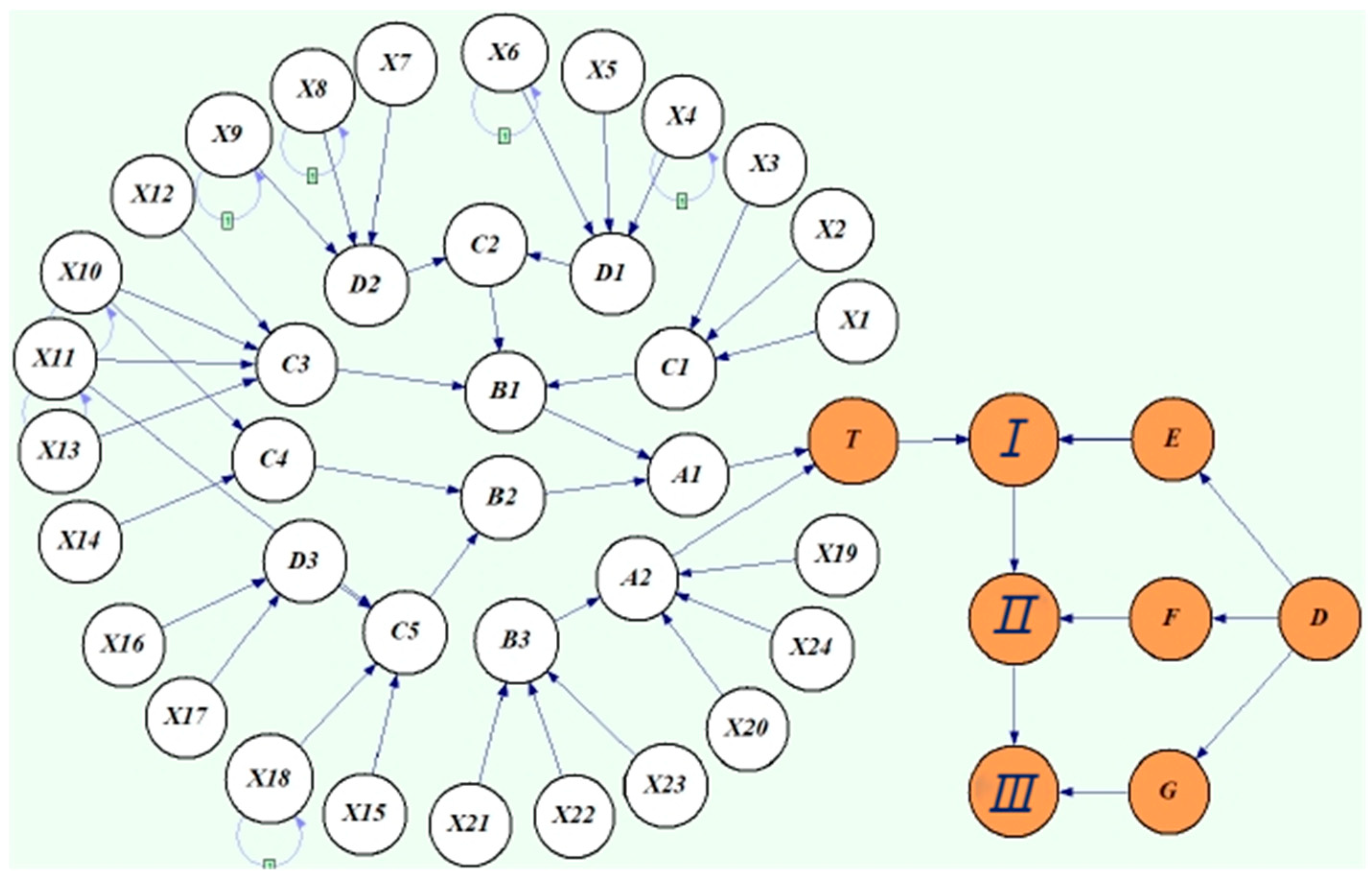
Figure 3.
Risk Warning Application Results.
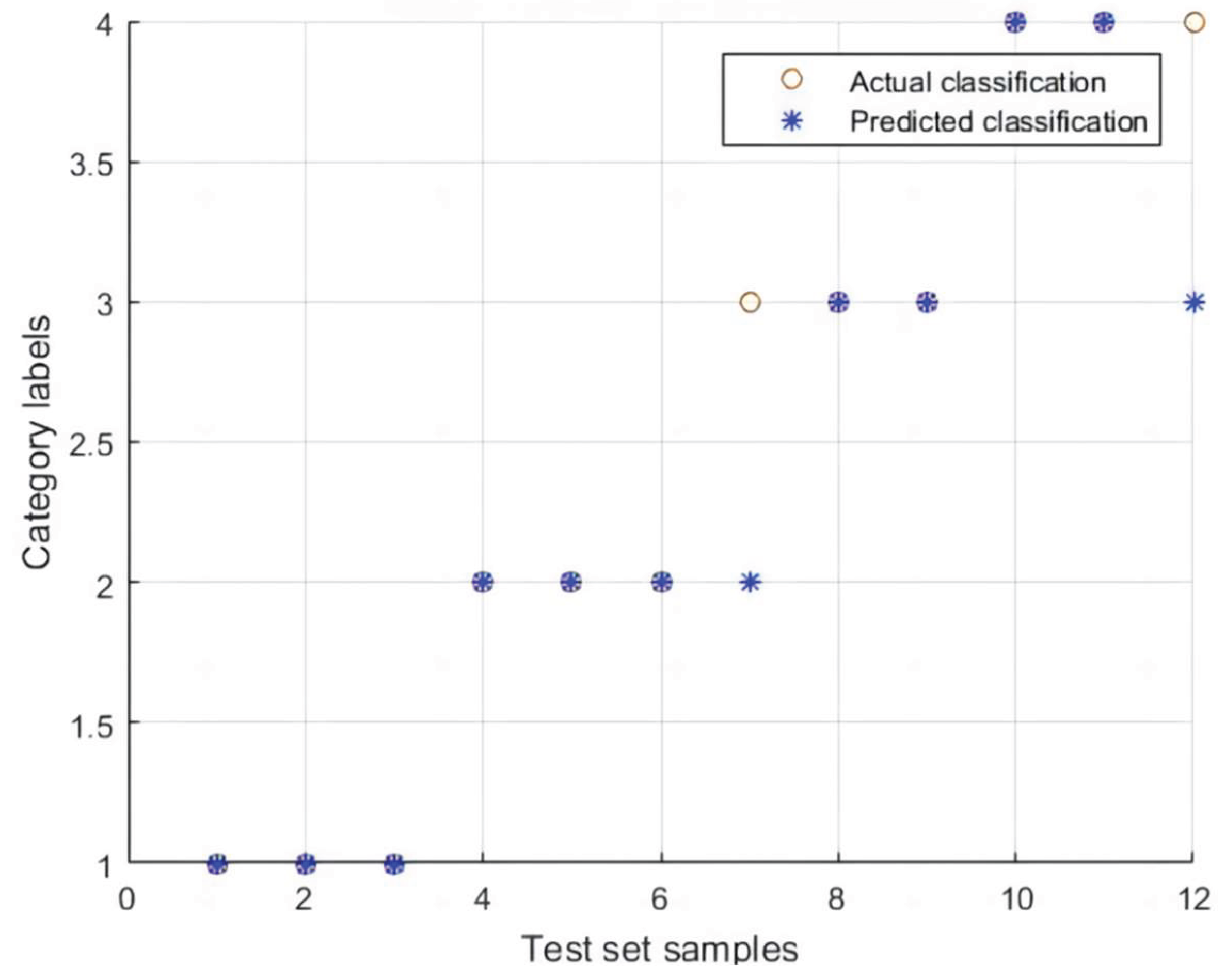
Table 2.1.
Probability Levels of Fire Scenarios.
| Probability | Level | Description |
| <0.0003 | A | Very Unlikely |
| 0.0003~0.003 | B | Unlikely |
| 0.003~0.01 | C | Occasional |
| 0.01~0.1 | D | Likely |
| 0.1~1 | E | Very Likely |
Table 2.2.
Severity Level Standards for Fire Consequences.
| Temperature (°C) | Severity Level |
| <150 | 1 |
| 150-200 | 2 |
| 200-300 | 3 |
| 300-400 | 4 |
| >400 | 5 |
Table 2.3.
Risk Assessment Matrix.
| Risk Level | Consequence Severity Level | ||||
| l | 2 | 3 | 4 | 5 | |
| <0.0003 | 1A | 2A | 3A | 4A | 5A |
| 0.0003~0.003 | 1B | 2B | 3B | 4B | 5B |
| 0.003~0.01 | 1C | 2C | 3C | 4C | 5C |
| 0.01~0.1 | 1D | 2D | 3D | 4D | 5D |
| 0.1~1 | IE | 2E | 3E | 4E | 5E |
Table 2.4.
Risk Level Classification Standards.
| Risk Level | Description | Explanation |
| I | Low Risk | 1A、2A、1B、1C |
| Ⅱ | General Risk | 3A、2B、3B、2C、1D、IE |
| Ⅲ | Moderate Risk | 4A、5A、4B、3C、2D、2E |
| IV | Major Risk | 5B、4C、5C、3D、4D、3E |
| V | Exceptionally Major Risk | 5D、4E、5E |
Table 3.1.
Judgment Matrix.
| Type | Circuit Breaker Failure | Overvoltage | Stray Current |
| Circuit Breaker Failure | (1,1,1) | (1/3,1/5,1) | (1,1/2,1) |
| (1/2,1/2,1) | (1/3,1/7,1) | ||
| (1/2,1/7,1) | (1/2,1/3,1) | ||
| Overvoltage | (1,5,3) | (1,1,1) | (1/3,1/5,1) |
| (1,2,2) | (1/3,1/9,1) | ||
| (1,7,2) | (1/2,1/7,1) | ||
| Stray Current | (1,2,1) | (1,5,3) | (1,1,1) |
| (1,7,3) | (1,9,3) | ||
| (1,3,2) | (1,7,2) |
Table 3.2.
Aggregated Judgment Matrix.
| Type | Circuit Breaker Failure | Overvoltage | Stray Current |
| Circuit Breaker Failure | (1,1,1) | (0.44,0.28,1) | (0.61,0.33,1) |
| Overvoltage | (1,4.67,2.33) | (1,1,1) | (0.39,0.15,1) |
| Stray Current | (1,4,2) | (1,7,2.67) | (1,1,1) |
Table 3.3.
Cable Overload Conditional Probability Table.
| Circuit Breaker Failure | Overvoltage | Stray Current | State1 | State0 |
| State1 | State1 | State1 | 0.73 | 0.27 |
| State1 | State1 | State0 | 0.35 | 0.65 |
| State1 | State0 | State1 | 0.36 | 0.64 |
| State1 | State0 | State0 | 0.29 | 0.71 |
| State0 | State1 | State1 | 0.46 | 0.54 |
| State0 | State | State0 | 0.14 | 0.86 |
| State0 | State0 | State1 | 0.17 | 0.83 |
| State0 | State0 | State0 | 0.0005 | 0.9995 |
Table 3.4.
Event Description and Basic Event Prior and Posterior Probabilities.
| Code | Description | A priori Probability | Posterior Probability | Code | Description | A priori Probability | Posterior Probability |
| X1 | Ventilation faults | 0.1056‰ | 0.1060‰ | X20 | Incendiary material fell into the compartment | 5.068‰ | 2.310‰ |
| X2 | Small cable spacing | 2.752‰ | 2.752‰ | X21 | Holes not sealed | 4.380‰ | 0.02245‰ |
| X3 | Poor cable compartment design | 97.52‰ | 9.774‰ | X22 | Fireproof paint not painted | 0.5156‰ | 0.02165‰ |
| X4 | Corroded joints | 0.1402‰ | 21.01‰ | X23 | Fire doors not closed in time | 15.63‰ | 9.000‰ |
| X5 | Poor installation quality | 0.8962‰ | 134.3‰ | X24 | Fire near cables | 35.25‰ | 2.570‰ |
| X6 | Insulation damage | 1.055‰ | 158.1‰ | A1 | Spontaneous combustion of cables | ||
| X7 | Breaker failure | 0.9600‰ | 143.8‰ | A2 | External ignition source | ||
| X8 | Overvoltage | 0.1881‰ | 27.13‰ | B1 | Cable core overheating | ||
| X9 | Stray current | 0.3153‰ | 4.724‰ | B2 | Arc fault | ||
| X10 | Long-term overload | 0.1938‰ | 29.04‰ | B3 | Fire extension | ||
| X11 | Deterioration of insulation | 0.1267‰ | 18.98‰ | C1 | Poor heat dissipation | ||
| X12 | Cable overlap | 0.9742‰ | 34.78‰ | C2 | Electricity leakage | ||
| X13 | Humid environment | 7.854‰ | 16.92‰ | C3 | Cable short circuit | ||
| X14 | Poor manufacturing process | 0.5350‰ | 2.410‰ | C4 | Exploding cable glands | ||
| X15 | Insufficient insulation thickness | 0.1938‰ | 29.04‰ | C5 | Insulation breakdown | ||
| X16 | Damaged installation | 4.390‰ | 118.3‰ | D1 | Bad connection | ||
| X17 | Animal damage | 12.27‰ | 129.9‰ | D2 | Cable overload | ||
| X18 | Reduced dielectric strength | 0.2713‰ | 40.65‰ | D3 | Damaged cable | ||
| X19 | Failure of electrical equipment | 3.270‰ | 117.9‰ |
Table 3.5.
Reliability of Cable Fire Control Measures.
| Code | Safety Barrier | Reliability |
| D | Automatic Detection System | 0.78 |
| E | Personnel Fire Extinguishing | 0.37 |
| F | Sprinkler Fire Extinguishing | 0.92 |
| G | Fire Brigade Fire Extinguishing | 0.51 |
Table 3.6.
Posterior Probabilities of Cable Trunk Safety State and Consequences.
| Risk factor categories | Risk factors | Corresponding basic events |
| Category I: patterns of change related to time factors | Related to cable overloading, connector corrosion | X4、X6、X8-X11、X18 |
| Category II: Stable existence of risk factors | Defects related to production, manufacturing, assembly | X2、X3、X5、X12、X14、X16、X20、X21、X22、X23、X24 |
| Category III: change patterns not related to time factors | Device-related failures, natural disasters | X1、X7、X13、X15、X17、X19 |
Table 3.7.
State Transition Matrix for X8 (Overvoltage).
| X8 | State0(t-1) | State1(t-1) |
| State0(t) | 0.75 | 0.11 |
| State1(t) | 0.25 | 0.89 |
Table 3.8.
Prior and Posterior Probabilities of Basic Events at the T9 Moment.
| Code | Descripción | A priori Probability | Posterior Probability | Code | Descripción | A priori Probability | Posterior Probability |
| X4 | Corroded connectors | 0.1402‰ | 25.49‰ | X10 | Long-term overloading | 0.1938‰ | 323.0‰ |
| X6 | Insulation damage | 1.055‰ | 136.4‰ | X11 | Aging of insulation | 0.1267‰ | 875.5‰ |
| X8 | Overvoltage | 0.1881‰ | 108.5‰ | X18 | Reduced dielectric strength | 0.2713‰ | 259.1‰ |
| X9 | Stray current | 0.3153‰ | 107.4‰ |
Table 3.12.
Risk Warning Application Sample Data.
| Warning Level | R1 | R2 | R3 | R4 | R5 | R6 | R7 | R8 | R9 | R10 |
| High Warning | Ⅱ | II | I | Ⅱ | IⅢ | IV | IV | II | Ⅱ | Ⅱ |
| I | I | I | III | I | IV | IV | I | Ⅱ | III | |
| Ⅱ | IV | I | Ⅱ | Ⅲ | IV | IV | II | Ⅱ | I | |
| Medium Warning | IⅡ | II | Ⅱ | Ⅱ | II | IV | IV | II | Ⅱ | Ⅱ |
| H | Ⅲ | Ⅱ | III | I | IV | IV | Ⅲ | Ⅱ | Ⅱ | |
| Ⅱ | II | Ⅱ | Ⅱ | II | III | IV | II | Ⅱ | Ⅱ | |
| Low Warning | Ⅱ | II | I | Ⅱ | II | III | IV | II | Ⅱ | Ⅱ |
| IV | II | Ⅱ | Ⅱ | II | III | IV | II | Ⅱ | Ⅱ | |
| IⅡ | IV | Ⅱ | Ⅱ | I | IV | IV | I | Ⅱ | III | |
| No Warning | II | I | I | III | I | IV | IV | IV | III | IV |
| II | II | I | III | II | IV | IV | IV | III | IV | |
| IⅡ | II | Ⅱ | Ⅱ | I | III | IV | II | III | Ⅱ |
Disclaimer/Publisher’s Note: The statements, opinions and data contained in all publications are solely those of the individual author(s) and contributor(s) and not of MDPI and/or the editor(s). MDPI and/or the editor(s) disclaim responsibility for any injury to people or property resulting from any ideas, methods, instructions or products referred to in the content. |
© 2025 by the authors. Licensee MDPI, Basel, Switzerland. This article is an open access article distributed under the terms and conditions of the Creative Commons Attribution (CC BY) license (http://creativecommons.org/licenses/by/4.0/).
Copyright: This open access article is published under a Creative Commons CC BY 4.0 license, which permit the free download, distribution, and reuse, provided that the author and preprint are cited in any reuse.


