Submitted:
07 June 2025
Posted:
09 June 2025
You are already at the latest version
Abstract
The objective of this study is to analyze spatial entropy flows that reveal the directional dynamics of climate change—patterns that remain obscured in traditional statistical analyses. This approach enables the identification of pathways for "climate information transport," highlights associations with atmospheric circulation types, and allows for the localization of both sources and "informational voids"—regions where entropy is dissipated. The analytical framework is grounded in a quantitative assessment of long-term climate variability across Europe over the period 1901–2010, utilizing Shannon entropy as a measure of atmospheric system uncertainty and complexity. The underlying assumption is that the variability of temperature and precipitation reflects the inherently dynamic character of climate as a nonlinear system prone to fluctuations. The analysis focuses on monthly distributions of temperature and precipitation, modeled using bivariate copula functions, with marginal distributions selected based on the Akaike Information Criterion. To enhance estimation accuracy, the study employs bootstrap techniques and numerical integration to compute Shannon entropy values at each of the 4,165 grid points, with a spatial resolution of 0.25° × 0.25°. The results indicate that entropy and its derivative are complementary indicators of atmospheric system instability—entropy proving effective in long-term diagnostics, while its derivative provides insight into short-term forecasting of abrupt changes. A lag analysis and Spearman rank correlation between entropy values and their potential support the investigation of how circulation variability influences the occurrence of extreme precipitation events. Particularly noteworthy is the temporal derivative of entropy, which reveals strong nonlinear relationships between local dynamic conditions and climatic extremes. A spatial analysis of the informational entropy field further uncovers well-defined structures of varying climatic complexity at the continental scale. This field appears to be clearly structured, reflecting not only the directional patterns of change but also the potential sources of meteorological fluctuations. A field-theory-based spatial classification allows for the identification of transitional regions—areas with heightened susceptibility to shifts in local dynamics—as well as entropy source and sink regions. The study is embedded within the Fokker–Planck formalism, wherein the change in the stochastic distribution characterizes the rate of entropy production. In this context, regions of positive divergence are interpreted as active generators of variability, while sink regions function as stabilizing zones that dampen fluctuations.

Keywords:
entropy transport
; entropy sources
; entropy sinks
; bootstrap method
; Fokker–Planck equation
; climate dynamics
; NOAA data
; monthly precipitation
; mean temperature
; Copula function
1. Introduction
Entropy, one of the fundamental concepts in physics, plays a pivotal role in the study of complex climate systems. In its thermodynamic formulation, it describes the degree of disorder and energy dissipation [1,2,3] while in Shannon’s information theory, it serves as a quantitative measure of uncertainty and complexity in data such as temperature and precipitation time series [1,4,5,6]. Contemporary research suggests a significant relationship between physical and informational entropy, opening new avenues for the quantitative assessment of climate variability [7,8].
The Earth’s climate system operates as an open, far-from-equilibrium system in which temperature and pressure gradients drive atmospheric and oceanic circulations [1,9,10]. These processes lead to the transport of heat and moisture and to the production of entropy—through energy dissipation, phase transitions, and diffusion [11]. Shannon entropy enables the evaluation of the system’s unpredictability, and its spatiotemporal analysis makes it possible to identify regions particularly susceptible to extreme weather phenomena [12,13,14].
In this study, we analyze spatial fields and entropy fluxes computed from monthly temperature and precipitation data, employing the formalism of gradients and divergence [1,2,15]. This approach allows us to capture the directional transport of climate information and to identify local structures of order and chaos that remain undetectable through conventional statistical methods [11,14,16]. The spatial variability of entropy gradients reflects dominant directions of climate variability flow and may indicate external influences such as the impact of the Atlantic Ocean or continentality gradients [17,18,19].
The correlation of entropy flux patterns with large-scale atmospheric indices (such as the NAO and AO) enables the linking of local variability patterns with global-scale phenomena [20,21,22]. Regions with elevated entropy relative to their surroundings act as variability generators, whereas areas with low divergence may function as stabilizers of the system, sensitive to external disturbances. Such spatial differentiation enables the identification of entropy sources, sinks, and informational gaps—elements crucial for climate monitoring and forecasting [10,12,23].
Classical analytical methods often fail to capture the nonlinear and stochastic aspects of atmospheric dynamics, particularly in Europe, where oceanic, continental, and Arctic influences converge [24,25]. The integration of information theory with phase space analysis, copula-based modeling, and vector analysis offers a refined framework for identifying these complex interactions [26,27,28]. The present study, grounded in prior work on thermodynamic entropy, chaotic dynamics, and copula theory, proposes a new methodological framework adapted to the climatic conditions of Europe [29,30,31,32]. The use of copula functions to model asymmetric dependencies between temperature and precipitation, along with the analysis of climate information transport, constitutes an innovative contribution to the development of tools for interpreting and forecasting climate variability [28,33].
2. Data Preparation for Analysis
The analysis presented in this study is based on high-quality gridded data published by the National Oceanic and Atmospheric Administration (NOAA [34,35,36]. The study area spans approximately 5,570 km × 4,050 km, covering latitudes from −10° to 40° and longitudes from 35° to 72°. For the purposes of this research, a uniform spatial resolution of 0.25° × 0.25° was applied consistently across all computations. The dataset comprises monthly mean temperatures and total monthly precipitation for the period 1901–2010 [34,37]. For each grid cell, individual time series of temperature and precipitation were extracted and served as the basis for subsequent analyses grounded in informational entropy.
The NOAA data were utilized at their original resolution, without re-interpolation or grid rescaling. A major reason for selecting this dataset was its temporal and spatial homogeneity. Both temperature and precipitation fields were developed using standardized interpolation algorithms and quality control procedures, applied consistently by the same institution. This ensures a high level of data integrity and facilitates comparability across regions and time periods.
To ensure the reliability of long-term trend analyses, NOAA datasets are routinely verified and homogenized. This includes statistical identification of anomalies, data gaps, and inconsistencies, as well as cross-validation with ground-based observations and satellite products [35,36,38,39]. As a result, the NOAA dataset provides a stable and trustworthy foundation for detecting climate variability signals associated with entropy flow, as well as for analyzing the spatial directions of climate information transport.
3. Methodology
This study investigates the relationships between the structure of informational entropy and extreme weather phenomena, with a particular focus on maximum temperatures and minimum precipitation totals [40,41]. The approach is based on the analysis of monthly entropy values and their spatial gradients (entropy potential) across a grid covering the European domain [2,12,21,42]. For each grid point, monthly values of informational entropy were calculated, derived from the joint distributions of atmospheric variables—namely temperature and precipitation [18,43]. Additionally, for each month, the spatial gradient of entropy was computed and interpreted as a vectorial entropy potential, with its magnitude (|∇Entropy|) serving as a proxy for local atmospheric variability and instability. The direction and rate of change in uncertainty across space are defined by the entropy gradient vector (∇Entropy) [44,45].
The primary objective of the analysis was to determine whether statistically significant relationships exist between entropy levels and their spatial dynamics, on one hand, and extreme values of maximum/minimum temperature and precipitation, on the other, at the same geographic locations. Three types of relationships were examined: (1) between the entropy value (Entropy) and weather extremes, (2) between the entropy potential (|∇Entropy|) and extremes, and (3) between the temporal derivative of entropy and extremes [41,44].
The first approach tested whether higher uncertainty levels (greater entropy) at a given location correspond with increased risk of high temperatures or drought. A positive correlation between entropy and maximum temperature would suggest that regions with higher variability are more prone to experiencing extreme heat events. Conversely, a negative correlation between entropy and minimum precipitation totals would imply that higher uncertainty favors the occurrence of severe droughts [24,46,47].
The second approach focused on the analysis of the entropy gradient, interpreted as the rate and direction of spatial entropy changes. The magnitude of the gradient vector (|∇Entropy|), or entropy potential, was used to identify regions of pronounced spatial instability that may serve as initiation zones for extreme events. The analysis thus examined whether sharp spatial variations in entropy are linked to the occurrence of extreme temperature and precipitation values [44,48,49].
All correlations were computed using two variants: temporal and seasonal–spatial. In the temporal analysis, for each grid point, the Spearman correlation was calculated between the 12-month entropy or entropy gradient series and the corresponding monthly values of weather extremes. The resulting correlation coefficient indicated the strength and direction of the relationship between monthly entropy fluctuations and variations in extreme weather events.
A high positive temporal correlation signified that months with elevated entropy potential coincided with months of extreme conditions (e.g., heatwaves), while a high negative correlation indicated an inverse relationship—i.e., that increased local instability was associated with lower extreme values, such as droughts. In the seasonal–spatial variant, spatial correlations were examined within each month separately. Spearman correlations were computed between the spatial distribution of entropy (or entropy gradients) and the spatial distribution of weather extremes for a given month [50,51]. This analysis addressed whether, during a given season, areas with higher entropy potential also exhibited a greater risk of extreme weather. These spatial correlations provided insight into the general seasonal–spatial structure of the relationship between climate variability and extremes [52].
To enhance the reliability of the results, the bootstrap method was applied. Repeated random sampling with replacement (1,000 iterations) yielded distributions of correlation coefficients and allowed for the assessment of their statistical significance. Based on these distributions, mean Spearman correlation values at a 5% significance level were computed, enabling an evaluation of the robustness of the findings [12,53,54].
The results were presented as spatial maps, including distributions of entropy, trends in entropy and entropy potential, temporal and seasonal–spatial correlation maps, and visualizations of entropy gradient streamlines. The streamlines indicated trajectories along which uncertainty propagates spatially—offering potential prognostic value. Particularly promising were the findings from the entropy gradient analysis, which pointed to the existence of spatial mechanisms that may initiate extreme weather events. Strong local entropy gradients may signal that the atmospheric system is approaching bifurcation thresholds that lead to more chaotic states.
4. Distribution Fitting
The methodology presented in this study is based on bivariate copula functions, which offer a coherent and statistically justified approach to modeling dependencies between random variables with arbitrary marginal distributions. This framework allows for the decoupling of marginal modeling from dependency structure modeling, thereby enhancing both flexibility and interpretability of the results.
The analytical process begins with the estimation of marginal distribution parameters using the Maximum Likelihood Estimation (MLE) method. MLE ensures estimator efficiency and consistency under standard regularity conditions. For each candidate marginal distribution, the Akaike Information Criterion (AIC) is applied to objectively select the best-fitting model, balancing model complexity against data fit [6,55].
The selected marginal distributions are subsequently transformed into the uniform space using their respective cumulative distribution functions (CDFs), a standard step in constructing copula functions. Next, the parameters of the selected copula families (e.g., Clayton, Gumbel, Frank, Gaussian, Student-t) are estimated, also using the MLE method [31,56,57]. This step enables a full characterization of the dependence structure, independently of the marginal distributions.
Among the fitted copulas, the one that best reproduces the observed dependencies in the data is selected, again using the AIC. This ensures the entire process is grounded in comparable and statistically robust measures of goodness-of-fit, eliminating arbitrariness in the choice of both margins and dependency structures. Such a methodology adheres to the standards of modern probabilistic modeling, integrating marginal and joint characteristics, and proves particularly useful in meteorological, hydrological, and financial applications.
Importantly, given a sufficiently large sample size and careful selection of candidate marginal and copula functions, this procedure enables not only the accurate description of dependencies but also the prediction of extreme events and the assessment of joint risks associated with their co-occurrence. The framework thus constitutes a coherent and calibratable approach for constructing bivariate probabilistic models with strong statistical foundations.
4.1. Marginal Distributions
The modeling of Shannon entropy in this study
relies on temperature and precipitation data. For each spatial grid cell,
marginal distributions were analyzed separately for monthly mean temperatures
and monthly total precipitation values.
- Generalized Extreme Value (GEV)
- Normal
- Log-normal
- Weibull
- Gamma
- Extreme Value
- Nakagami
Each of these distributions was fitted using the Maximum Likelihood Estimation method, supplemented by ADT tests, and the optimal model selection was based on AIC values. This selection process accommodates local climatic variability and the differing characteristics of temperature and precipitation across various regions of Europe.

Table 1.
Analyzed distribution forms for temperature and precipitation variables [57].
Table 1.
Analyzed distribution forms for temperature and precipitation variables [57].
| Distribution Name | Mathematical Form | Distribution Parameters | No eq.. |
| Generalized Extreme Value | for >0 and | -- location parameter, scale parameter and shape parameter | (1) |
| Normal | x –random variable, standard deviation, and mean | (2) | |
| Lognormal | for | x –random variable and distribution parameters | (3) |
| Weibull | - random variable, standard deviation, and mean | (4) | |
| Gamma | - random variable, distribution parameters, and the Gamma function | (5) | |
| Extreme Value | -- location parameter, scale parameter | (6) | |
| Nakagami | for | – shape parameter, scale parameter | (7) |
4.2. Bivariate Copula Functions
Due to their flexibility in coupling arbitrary marginal distributions within multivariate probability structures and their favorable computational properties, copula theory was employed in this study [58,59,60]. The selection of a specific copula function—analogous to the procedure for choosing marginal distributions—was based on a predefined set of bivariate copulas: Gaussian, Clayton, Frank, and Gumbel (Table 2), with the final choice determined using the Akaike Information Criterion (AIC) [33,60,61,62]. The Gaussian copula assumes symmetric dependence between variables, which renders it suboptimal for modeling the frequently observed asymmetric and nonlinear relationships between precipitation and temperature under European climatic conditions. In contrast, the Clayton copula captures strong dependencies in the lower tail of the distribution, which is particularly relevant for analyzing phenomena such as droughts—that is, the simultaneous occurrence of extremely low precipitation and high temperatures.
Alternative copula functions, such as the Gumbel copula (favoring upper-tail dependence) or the Frank copula (appropriate for moderate, symmetric correlation), exhibit lower suitability for the analyzed data due to their inability to capture the asymmetric dependency structures characteristic of extreme events. The selected set of copula functions was well-suited to the empirical characteristics of the temperature and precipitation data, allowing for precise modeling of their joint variability, including cases of extreme co-occurrence.
5. Shannon Entropy as a Measure of Climate Information
Shannon entropy, though originally derived from information theory, is widely applied in environmental and climate data analyses as a nonparametric measure of uncertainty, disorder, and variability in probability distributions. In climatological literature, informational entropy has been successfully used to analyze seasonal and spatial climate variability, as well as to detect shifts in weather regimes. In the present approach, emphasis is placed on the empirical evaluation of entropy’s evolution across time and space as an indicator of local climate instability—without requiring reference to an external or idealized distribution [63]. Defining such a “reference” distribution can be challenging, if not impossible, in the context of complex and nonlinear atmospheric processes. Under conditions of high meteorological variability and spatial heterogeneity, adopting an arbitrary reference distribution may lead to ambiguous or misleading interpretations.
For this reason, a self-contained approach based on empirical entropy was adopted. It enables tracking the degree of order in weather data without relying on additional model assumptions, thereby enhancing the method’s universality and robustness against errors arising from incorrect distributional specifications. In informational terms, an increase in Shannon entropy reflects a higher level of randomness and complexity in the distribution of climate variables, which directly translates into reduced predictability of weather conditions and, potentially, greater vulnerability of the system to extreme events. Thus, the use of entropy as an indicator for analyzing climate variability aligns with the growing interest in nonparametric measures of uncertainty that allow for the assessment of irregularities and risk within a dynamically changing climate system.
Shannon entropy quantifies the uncertainty associated with predicting the value of a random variable [5,27,64]. It is calculated from the estimated probability distribution, and the accuracy of this estimate directly influences the reliability of the entropy computation. An improperly selected or poorly fitted distribution may result in erroneous entropy values, potentially leading to incorrect conclusions about the underlying climate structure.
The formula for Shannon entropy of a continuous bivariate random variable , with joint probability density function , is defined as [26,65,66]:
Here, is the joint PDF of the bivariate distribution derived from the copula and marginals. Marginal PDFs and . Copula density , which is derived from the zbioru postaci różnych copula.
The formula for the joint PDF becomes:
Use the definition:
to estimate the entropy as the negative mean of the log joint PDF.
In discussing units of Shannon entropy for
continuous distributions, the results are typically expressed in units of
information—nats (when
natural logarithms are used) or bits
(when base-2 logarithms are used). The choice of unit depends on analytical
conventions and the logarithmic system employed [12].
To preempt known criticisms and limitations
associated with the use of Shannon entropy, this study was designed with
methodological rigor. Measures implemented included:
- standardization of measurement units across the entire dataset,
- consistent estimation of marginal distribution parameters using the Maximum Likelihood Estimation (MLE) method,
- and uniform discretization procedures for all input data.
The selection of both marginal distributions and
copula functions was guided by the Akaike Information Criterion (AIC), allowing
for an objective assessment of model fit under consistent modeling assumptions.
These methodological safeguards ensured the integrity of the entire procedure,
aligning it with the rigorous standards required in climate data
analysis—particularly in the context of studying extreme weather events and
their relationship to informational measures of uncertainty, such as entropy.
6. Entropy Fluxes as a Tool for Spatiotemporal Analysis of Climate Variability
In the analysis of extreme weather phenomena—such
as heatwaves, droughts, or flash floods—information-theoretic metrics,
particularly informational entropy, are increasingly being employed [45,67]. The proposed approach extends classical
entropy analysis by incorporating field-based aspects: spatial gradients,
divergence, and the associated entropy flux [68].
The introduction of operators known from continuum physics (such as ) enables a mathematical representation of
informational flows between adjacent cells of the analytical grid [69]. This serves as a foundation for detecting
sources and sinks of climate variability. In particular, extreme events may be
preceded by changes in the informational structure of the atmospheric system,
whose spatiotemporal patterns can be captured through the analysis of entropy
fluxes [15,70].
Informational entropy is not a classical energy
function but rather a measure of informational disorder—making its diffusion
conceptually different from classical heat diffusion. The interpretation of
“information flux” as the spatial derivative of entropy is metaphorical yet
statistically valid, provided it is understood as a representation of
statistical structure, rather than a literal physical energy transfer. It is
essential to emphasize that in the context of “climate information,” the term
refers to the statistical structure of weather variability, not to concrete
datasets [71].
This study presents a framework based on the
spatiotemporal analysis of informational entropy distributions aimed at
understanding the dynamics of extreme climate events. Each geographic grid cell
(with a resolution of 0.25° × 0.25°) is assumed to hold a value of entropy , calculated from meteorological variables
describing local conditions. This entropy can be interpreted as a measure of
uncertainty or complexity of the climatic regime at a given location and time.
The spatial gradient vector of entropy, , indicates the direction and intensity of uncertainty change
across space, while its orientation reveals the direction in which structural
changes in information propagate.
The entropy flux is then defined as:
representing a hypothetical flow of climate information between neighboring cells, analogous to diffusion mechanisms in physics. The divergence of this flux,
allows the identification of areas that act as sources or sinks of variability, which can be critical in detecting spatial dynamic regimes. This formalism is grounded in classical field theory and employs well-established mathematical tools of vector calculus (gradient, divergence, Laplacian). Applying this methodology to meteorological data enables the identification of regions with elevated instability, which may serve as precursors to extreme weather events.
In particular, the temporal derivative of entropy, , serves as an indicator of local atmospheric system dynamics, where sharp increases may signal impending destabilization, such as intense precipitation or heatwaves. This approach effectively integrates classical concepts of information with climate process analysis and introduces a novel dimension to the detection and prediction of environmental hazards [44].
6.1. The Informational Entropy Field
For the informational entropy function derived from the bivariate distribution of temperature and precipitation variables at a given spatial point , the time-window-based estimate can be expressed as:

For each grid cell with geographical coordinates at time , the concept of the spatial entropy gradient vector is introduced as:
where denote partial spatial derivatives of entropy along the west–east and south–north axes, respectively. This gradient reflects both the direction and intensity of local informational complexity changes in space. The entropy flux vector is defined analogously to classical diffusion:
where is the entropy diffusion coefficient, which may be treated either as a fixed empirical constant or as a function of local environmental conditions.
Further analysis relies on the divergence operator; sources and sinks of entropy in space are identified via the divergence of the entropy flux vector:
When , positive divergence values indicate areas (grid cells) acting as sources of information, or generators of variability.
When ,, negative divergence values indicate absorbers of variability, associated with relative atmospheric stability.
6.2. Relationship with Weather Extremes
Climatic extremes can be analyzed through the lens of local entropy stability. Stability is quantified by examining temporal changes in entropy:
Persistently low entropy values with weak spatial gradients suggest a stable weather regime—a potential predictor of droughts or heatwaves. Conversely, a sharp increase in the entropy time derivative signals regime destabilization, serving as a predictor of floods or severe storms.
The concept of entropy flux offers a novel perspective on climatic processes as a dynamic system of information exchange between neighboring regions. Areas with strong positive divergence may indicate localized instabilities conducive to extreme events—such as the initiation of convective storms or surface overheating under weak circulation conditions. In contrast, regions with negative divergence may correspond to stabilizing zones, for example, persistent high-pressure systems that sustain stable weather conditions.
This spatial differentiation enhances understanding of which regions act as sources or sinks of variability over a given period, with direct implications for risk assessment of extreme weather events.
Beyond spatial aspects, the temporal derivative of entropy provides insight into the stability of local weather regimes. An increase in this derivative can be interpreted as a signal of destabilization and growing unpredictability of the system—conditions that often precede the onset of climatic extremes. The combined assessment of spatial entropy gradients and the temporal evolution of entropy and its derivatives delivers a more comprehensive picture of atmospheric system dynamics [72].
7. Statistical Tests Used
To assess trends in Shannon entropy for both precipitation and temperature, the bootstrap resampling technique was employed to generate multiple statistical realizations and to estimate stable entropy values. For each iteration, a separate estimation of the marginal distribution parameters was performed, followed by the construction of a joint distribution using copula functions.
The characteristics and patterns of entropy trends were analyzed using the Mann–Kendall test (MKT), a nonparametric statistical test widely used in climate change studies [73,74]. Trends were evaluated at a 5% significance level. In addition, the Pettitt test (PCPT) was applied to detect changepoints in the time series of entropy. This test was also conducted at a 5% significance level.
If a changepoint was confirmed at this level of significance, the time series was divided into subsequences, each of which was then reanalyzed for trends using the Mann–Kendall test. In cases where no changepoint was detected, the test was applied to the entire sequence [50,53,75].
To quantify the strength of the trend, a nonparametric slope estimator proposed by Sen and extended by Hirsch was used, which calculates the median of pairwise changes over time [76,77,78]. This approach allowed not only for detecting the presence of a trend but also for determining its direction and magnitude.
Marginal distributions describing temperature and precipitation for each analyzed sequence were estimated using the Maximum Likelihood Estimation (MLE) method, assessed with the Anderson–Darling test (ADT), and the optimal model was selected based on the Akaike Information Criterion (AIC).
In this study, the Pettitt test was specifically applied to identify changepoints in the time series of Shannon entropy derived from monthly precipitation totals and average monthly temperatures. PCPT, based on a test statistic compared against a critical value, allowed for determining whether the null hypothesis of no abrupt change could be rejected [75]. This method is widely used in climatological and hydrological analyses due to its robustness in detecting structural changes in environmental time series [12].
8. Results of the Analyses and Discussion
To accurately assess trends in informational entropy for precipitation and temperature, the bootstrap resampling method was employed to generate multiple realizations of Shannon entropy. The entropy calculations were based on the bivariate joint probability distribution of temperature and precipitation (Figure 1).
From the resulting time series of entropy values, seasonal trends were computed, and their statistical significance was evaluated using the Mann–Kendall test (MKT) at a 5% significance level. Additionally, to detect potential changepoints in the trend trajectories, the Pettitt test (PCPT) was applied, also at a 5% significance level.
If the presence of a changepoint was confirmed, each newly segmented subsequence was analyzed separately for trends using the MKT. If no changepoint was identified, the trend was assessed over the entire sequence.
The results were presented graphically, providing a clearer and more precise visualization of changes in entropy values and the evolution of their trends. For comparative purposes, the Shannon entropy values were normalized to the range (0, 1). The original entropy range—computed via integration from the joint bivariate probability distribution based on a sample size of 70 (T, P) pairs—spanned from 0 to 12.259 bits. This normalization allowed for consistent interpretation of spatial and temporal patterns of variability.
The meteorological entropy analysis, conducted separately for each calendar month, was based on long-term data from 1901 to 2010. This allowed for the averaging of seasonal patterns of weather variability across Europe. Calculations for each of the 40 analyzed years were based on 70-year seasonal time series: for the year 1971, the period 1901–1970 was used; for 1972, the period 1902–1971; and so on, up to 2010, for which data from 1941–2010 were used.
Each of the 12 panels in the graphical analysis corresponds to a calendar month, from January (top left) to December (bottom right). The color scale reflects the magnitude of entropy: from the lowest values (light yellow – low weather variability) to the highest (dark purple – high variability).
In January, low entropy values dominate across Northern Europe, indicating stable and predictable winter conditions. Elevated entropy values appear locally in the south—particularly over the Iberian Peninsula, southern France, and the Mediterranean regions—where precipitation variability is higher.
In February and March, similar patterns persist, although the zone of increased entropy gradually shifts toward Central Europe. April shows growing spatial differentiation, particularly over the Alps, the Balkans, and Southeastern Europe. In May, a general decline in entropy is observed, reflecting the typical springtime stabilization of the atmosphere.
Entropy peaks in June and July, especially across Southeastern Europe—including the Balkans, Greece, Turkey, and Northern Africa—likely linked to intensified convective storm activity and localized precipitation events. In August, high entropy zones shift northward, covering parts of southern Germany, Poland, and Ukraine.
In September, variability moderates in Western Europe, while remaining elevated in continental regions. October brings a further decline in entropy over Northern and Central Europe, though high values persist in the Mediterranean basin. In November, entropy decreases across most regions, remaining moderate only in Southeastern Europe. December, like January, is marked by low entropy across nearly all of Europe, associated with dominant, stable winter synoptic patterns.
The observed spatial patterns of entropy reveal a pronounced seasonal rhythm: minimal variability during winter and peak variability during summer, especially in the southern and southeastern parts of the continent. High entropy in the warmer months reflects the intensification of convective processes and increased atmospheric instability.
Mountainous regions—such as the Alps and Carpathians—exhibit elevated entropy values throughout much of the year, indicative of complex orographic conditions and local microcirculations. In contrast, the Mediterranean coasts show high variability particularly in autumn and winter, associated with episodic Mediterranean cyclones. Scandinavia and Northeastern Europe display the lowest entropy values for most of the year, confirming their stable and strongly seasonal climatic character.
9. Trend and Seasonal Variability of Shannon Entropy in the Context of Climate Change
The spatial distribution of meteorological entropy trends, calculated separately for each calendar month, is presented in Figure 2. Each of the 12 panels corresponds to a specific month. The color scheme illustrates the direction and magnitude of entropy trends—shades of red and orange indicate statistically significant increasing trends, while shades of blue denote decreasing trends. The statistical significance of the results was assessed using the Mann–Kendall test at a 5% significance level.
In January, positive trends (yellows and light oranges) dominate, particularly across Central Europe and Scandinavia, which may indicate increasing variability in winter weather conditions. February displays a greater number of negative trends in Southeastern Europe and the Alpine region, possibly reflecting a stabilization of local winter climates.
In March, distinctly positive trends appear in Germany, Poland, Scandinavia, and northern France, suggesting a rise in weather variability during the early spring period. April presents a more spatially scattered trend pattern, though positive values still prevail across Central and Eastern Europe.
May exhibits particularly strong positive trends in the Black Sea basin, the Balkans, and western Russia. June shows widespread positive trends across most of Europe, indicating a rise in atmospheric instability associated with the onset of summer.
In July and August, positive trends dominate Northern and Central Europe, while the southern parts of the continent show more areas with no statistically significant changes. September reveals decreasing entropy trends in Spain, Portugal, and southern France, while positive trends persist in the northern parts of the continent.
In October, entropy increases are especially prominent in Eastern Europe, including the Baltic states and western Russia. November brings marked positive trends in Central and Eastern Europe, along with localized decreasing trends in the western regions. In December, strong positive trends dominate across Northern Europe, with additional increases observed locally in the Alpine and Balkan regions.
Figure 3 presents the spatial distribution of the year in which a statistically significant change in meteorological entropy trend occurred, as determined using the Pettitt Change Point Test (PCPT) at the 5% significance level. Each of the twelve panels corresponds to a calendar month, from January (top left) to December (bottom right). The colors on the maps indicate the year in which the change point was detected—ranging from 1971 (dark blue) to 2010 (red)—while white areas represent grid cells where no statistically significant trend change was observed.
In January, the majority of change points occur after 1990, particularly across Central and Northern Europe. February displays a more dispersed pattern, with many change points falling between 1980 and 1995, especially in the Balkans and Southwestern Europe. In March, trend changes tend to occur earlier—often in the 1970s—predominantly over the Alpine region, Germany, and France. April exhibits a concentration of change points around 1990, especially across Central and Eastern Europe.
In May and June, red and orange hues dominate, indicating that the entropy trend changes tend to occur near the end of the analysis period (1995–2010). July and August display more spatially and temporally heterogeneous distributions of change points, suggesting that localized processes may be influencing entropy during the summer season.
In September, relatively early change points are observed, particularly in Northern Scandinavia and parts of Western Europe. October and November are characterized by a dense clustering of change points in Central and Northern Europe, primarily during the 1985–2000 period. December shows a prevalence of late-occurring changes, concentrated mostly in Southeastern Europe.
Mountain regions, such as the Alps and Carpathians, frequently exhibit earlier occurrences of change points, which may reflect a heightened sensitivity of entropy to shifting climatic conditions in orographically complex areas. In contrast, the absence of detected change points in regions such as Northern Scandinavia or Southern Spain suggests a relative stability of entropy trends in those areas.
The identified change point patterns also exhibit a seasonal character: during winter months, changes are more likely to occur in the final two decades of the study period, whereas during spring and autumn, the majority of change points cluster in the 1980s and 1990s.
10. Temporal Spearman Correlations
In this study, we analyze the spatial flows of informational entropy, computed from climate data on a grid with a resolution of 0.25° × 0.25°. The adopted approach enables the identification of subtle, directional patterns of climate variability that often remain undetected when using conventional statistical methods.
Below, we present correlation maps between meteorological entropy and selected climate parameters. The color scale on the right side of each map indicates the strength and direction of the correlation: warm colors (yellow, orange, red) represent positive correlations, while cool colors (various shades of blue) correspond to negative correlations.
10.1. Spatial Relationship Between Entropy and Monthly Maximum Temperature
The Spearman correlation map between informational entropy and monthly maximum temperature (Figure 4) reveals clear spatial variability in their relationship. In Southern Europe—particularly over the Iberian and Apennine Peninsulas, Greece, and Turkey—strong positive correlations dominate, locally exceeding 0.6. This suggests that increased atmospheric irregularity is associated with the occurrence of extremely high temperatures, which is typical of the Mediterranean climate regime.
In Central and Northern Europe (Germany, Poland, the Baltic States), correlations are weak or near zero, possibly reflecting the dominance of other climatic drivers. Scandinavia and the North Sea region also show positive correlations, although more limited in extent. Mountain regions (the Alps, Carpathians, and Pyrenees) display strong local contrasts, likely influenced by orographic effects. A patchwork of correlations is observed in Eastern Europe (Ukraine, Russia), indicating the absence of a unified mechanism. In parts of France and Italy, notable negative correlations appear, suggesting that higher entropy may coincide with lower maximum temperatures.
Overall, the spatial pattern indicates that the relationship between entropy and extreme temperatures is particularly pronounced in regions characterized by high seasonality and thermal instability.
10.2. Spatial Relationship Between Entropy and Monthly Minimum Temperature
The correlation pattern with minimum temperature (Figure 4) differs significantly from that observed for . In Southeastern Europe (Greece, Bulgaria, Turkey, and the Black Sea coast), strong negative correlations dominate, implying that higher entropy may be associated with nighttime cooling and an increased risk of low values.
In Central Europe, correlations are more variable—often close to zero, occasionally negative. In Scandinavia and northern Russia, weak positive correlations prevail, which may reflect a buffering effect of atmospheric variability on temperature drops. Mountain regions (Alps, Carpathians) exhibit strong local contrasts, likely due to microscale processes and topographic complexity. Neutral relationships dominate in Western Europe (France, Germany), while the Iberian Peninsula displays considerable heterogeneity, with both positive and negative values.
The relationship between entropy and is especially relevant in the context of frost risk and agricultural impacts. In arid and mountainous regions, strong negative correlations suggest the need for localized microclimatic analyses.
10.3. Spatial Relationship Between Entropy and Monthly Maximum Precipitation
The map of entropy correlations with monthly maximum precipitation totals (Figure 4) reveals a predominance of positive correlations across Central and Northern Europe (Germany, Poland, the Baltic States, Scandinavia). This indicates that higher entropy may be linked to increased risk of high-precipitation months, often associated with cold fronts and cyclonic activity.
In Southern Europe (Spain, Italy, Greece), negative correlations prevail, suggesting that in these regions, increased atmospheric variability does not correspond to greater monthly precipitation maxima—likely due to the influence of summer dry seasonality. Mountain areas (Alps, Pyrenees) display a diverse range of correlation values, reflecting local effects such as orographic lifting and convective storms. Western Europe (France, the British Isles) shows localized positive correlations.
In many temperate regions, correlations exceed +0.4, indicating the potential of entropy as an indicator for extreme precipitation risk.
10.4. Spatial Relationship Between Entropy and Monthly Minimum Precipitation
Correlations between entropy and monthly minimum precipitation totals (Figure 4) reveal a distinct north–south contrast. In Southern Europe (Spain, Italy, Greece, Turkey), strong negative correlations dominate, indicating a link between high entropy and increased drought risk. In Western and Central Europe, correlations are generally weak or neutral.
In Scandinavia and the British Isles, weak positive correlations prevail, suggesting that atmospheric variability does not directly translate into dry months in these regions. Areas around the Black Sea exhibit negative correlations, likely due to strong precipitation seasonality and local circulation patterns.
In mountainous regions (Alps, Carpathians, Pyrenees), as well as in Southern Spain and Sicily, strong local negative correlations appear, indicating that entropy may be a reliable indicator of monthly drought risk. Urban areas (e.g., London, Paris, Berlin) do not exhibit significant anomalies.
10.5. Spatial Relationship Between Entropy Gradient and Monthly Maximum Temperature
The Spearman correlation map between the entropy gradient and monthly maximum temperature (Figure 5) reveals strong regional contrasts. In Southeastern Europe (Turkey, Greece, and the Balkans), dominant strong positive correlations (>0.6) indicate a link between local variability changes and susceptibility to heatwaves. In these regions, the entropy gradient may reflect growing thermal instability.
In Central and Western Europe, correlations are predominantly negative or near zero, suggesting the stabilizing effect of a temperate climate. The Alps and southern Germany exhibit strong negative correlations, potentially indicating that increases in entropy gradients are associated with reductions in temperature extremes.
In Scandinavia (Norway and Sweden), positive correlations are observed, possibly reflecting the high sensitivity of the boreal climate. The Benelux countries, France, and the British Isles show values close to zero, while localized positive correlations appear in Italy, Ukraine, and Romania—regions that may serve as transitional zones between maritime and continental climatic influences.
Topography emerges as a significant factor: in mountainous areas, entropy gradients often display an inverse relationship with temperature compared to lowland regions.
10.6. Spatial Relationship Between Entropy Gradient and Monthly Minimum Temperature
The correlation map between the entropy gradient and minimum temperature (Figure 5) reveals strongly negative values in Southeastern Europe—particularly Turkey, Greece, and the Balkans—reaching below –0.6. This suggests that increasing variability may be associated with intensified cold nights, likely due to inversions or radiative cooling effects.
In Western Europe, correlations are near zero, while in the Alps and Carpathians, localized positive values appear—likely influenced by terrain features and local atmospheric dynamics. Scandinavia exhibits moderate positive correlations, which may indicate the dampening of cold extremes under increased instability.
In the Adriatic region, the entropy gradient shows strong negative correlations with TminT_{\text{min}}Tmin, possibly driven by advective cooling. In Central Europe (Poland, Germany, Czechia), a mosaic pattern emerges, likely due to seasonal shifts in the influence of precipitation and snow cover.
The entropy gradient may serve as an indicator of frost risk, though the relationship is not uniform and requires seasonal analysis—particularly in winter months.
10.7. Spatial Relationship Between Entropy Gradient and Monthly Minimum Precipitation
The analysis of the entropy gradient’s correlation with minimum monthly precipitation (Figure 5) reveals a predominance of negative relationships in Southern Europe—especially in Spain, southern France, Greece, Italy, and Turkey. Values below –0.4 suggest a connection between increasing spatial variability and the risk of drought conditions.
In Central Europe (Poland, Czechia, Germany), correlations are weak or neutral. In Scandinavia and the North Sea region, positive correlations are more common, suggesting greater precipitation stability despite increased entropy gradients.
Localized positive correlations are observed in the Alps and Carpathians, while positive values dominate in Eastern Europe (Ukraine, Russia), indicating a more continental-type response of precipitation to spatial variability.
Overall, the entropy gradient appears useful in detecting regions vulnerable to drought, particularly in the Mediterranean basin.
10.8. Spatial Relationship Between Entropy Gradient and Monthly Maximum Precipitation
Correlations between the entropy gradient and monthly maximum precipitation (Figure 5) are generally positive across temperate regions—especially in Germany, Poland, the Baltic States, and Western Russia—ranging from 0.2 to 0.6. This suggests that spatial instability is associated with the intensification of extreme precipitation episodes.
Scandinavia (Norway and Sweden) also shows positive correlations. In Southern Europe (Spain, Italy, Greece), correlations are mostly negative or neutral, likely due to strong seasonality and limited spatial variability during dry periods.
Urban areas (e.g., London, Paris, Berlin) and mountain regions (e.g., the Alps) exhibit moderate positive relationships. The entropy gradient thus emerges as a sensitive indicator of spatial rainfall dispersion, potentially valuable for assessing flash flood risk.
11. Seasonal–Spatial Spearman Correlations
11.1. Analytical Approach
A spatial-seasonal analysis was performed on the maximum absolute values of Spearman rank correlations between meteorological entropy (incorporating monthly temperature and precipitation) and extreme climate parameters. Time lags from 1 to 12 months were considered to evaluate the predictive potential of entropy in anticipating climate changes.
11.2. Entropy and Monthly Minimum Temperature
Figure 6 presents maps of maximum absolute correlations (left panel) and the corresponding time lags (right panel). In Central-Eastern Europe and Scandinavia, positive correlations dominate (ranging from 0.4 to 0.6), suggesting that increases in entropy precede declines in . In contrast, negative correlations are observed in Southern Europe (Spain, Italy, Greece), indicating the inverse relationship.
The most frequent lag values fall between 6 and 10 months, pointing to the seasonal nature of the observed interactions. In higher latitudes (above 60°N), correlations remain positive, with shorter lags (3–5 months), reflecting the more immediate response of boreal climates. The spatial consistency of 6–9 month lags across Central-Eastern Europe may indicate the presence of a semiannual climatic memory mechanism.
11.3. Entropy and Monthly Maximum Temperature
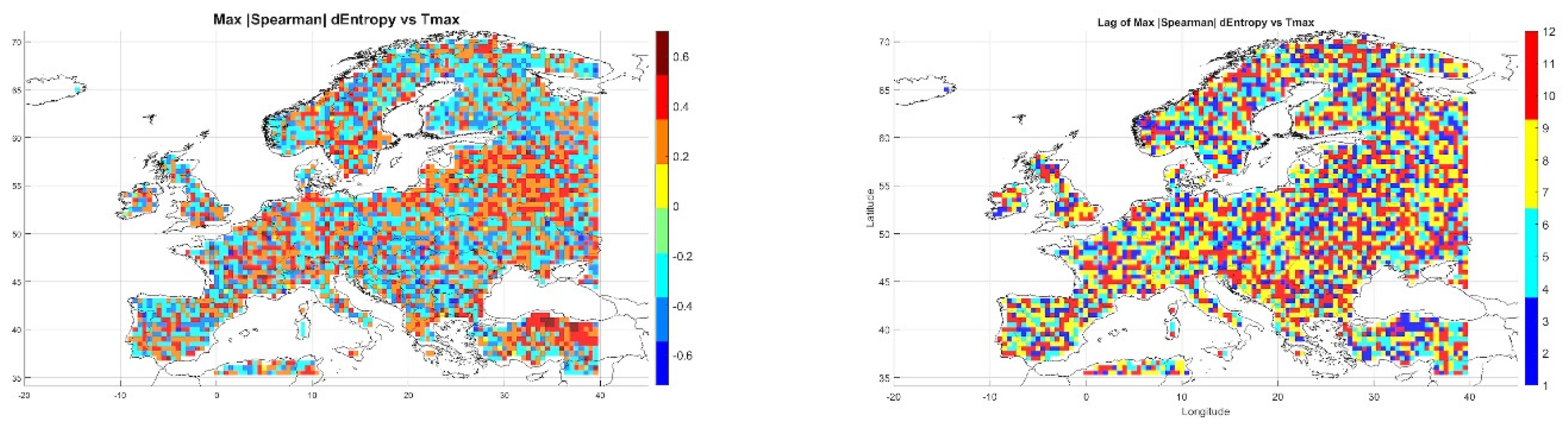
Figure 7 presents an analogous analysis for . Strong positive correlations (>0.4) are observed in Central-Eastern Europe and Scandinavia, suggesting that entropy is a reliable indicator for forecasting episodes of elevated temperatures. In Southern Europe, negative correlations dominate, possibly reflecting local damping mechanisms.
The strongest associations occur with time lags of 6–9 months. Western Europe shows greater spatial variability and generally weaker correlations, likely due to oceanic influence and seasonal instability. The similarity in lags between and points to the seasonal consistency of the system’s response. However, regional differences in correlation strength and direction highlight the need for localized modeling approaches for maximum temperatures.
11.4. Entropy and Monthly Minimum Precipitation
Figure 8 illustrates the spatial distribution of correlations and time lags between entropy and . Positive correlations (>0.4) prevail across Central and Northeastern Europe, indicating that entropy anomalies precede periods of reduced rainfall. In Southern Europe (Spain, Greece, Turkey), negative correlations (down to –0.6) dominate, suggesting distinct climatic dynamics in these regions.
The strongest correlations occur at lags of 6–10 months, while in Southern Europe the lags are shorter (<4 months). Eastern Europe exhibits a high degree of lag regularity, potentially indicating a stable climatic rhythm. In countries such as Poland, Ukraine, and Finland, entropy may serve as a strong predictor of drought conditions. Variability in mountainous areas may be influenced by orographic effects.
11.5. Entropy and Monthly Maximum Precipitation
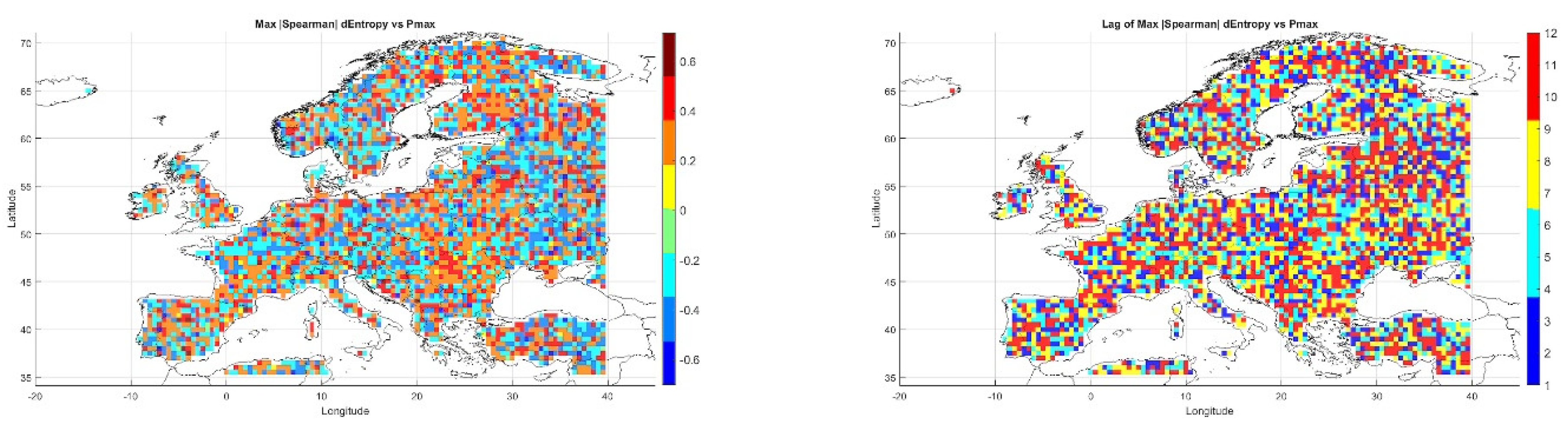
Figure 9 presents the relationship between entropy and monthly precipitation maxima. Positive correlations (>0.4) dominate across Central and Eastern Europe, with local maxima up to 0.8 observed in southern Germany, Austria, and the Czech Republic—where increased entropy precedes intense precipitation events.
The strongest correlations are found at 6–9 month lags, with several regions also showing peaks at 12 months, suggesting the existence of annual precipitation cycles. In the Mediterranean basin, correlations are weaker or even negative, likely due to seasonal dryness and irregular atmospheric dynamics. High correlations in mountainous regions (Alps, Carpathians) suggest that topography significantly modulates the precipitation response to entropy variability.
11.6. Summary
Meteorological entropy shows strong delayed
associations with extreme values of temperature and precipitation. The highest
positive correlations are observed in Central Europe, Scandinavia, and parts of
Eastern Europe. The most common time lags are in the 6–9 month range,
indicating a seasonal translation of entropy variability into climate
parameters. Topography and local factors (e.g., oceanic climate, seasonal
circulation) significantly influence the strength and direction of these
relationships. Entropy may function as an early proxy for predicting , offering potential applications in climate
modeling and early warning systems for extreme weather events.
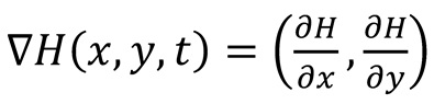
11.7. Temporal Derivative of Entropy and Minimum Temperature
Figure 10
displays the maximum absolute Spearman correlations between the temporal
derivative of entropy and monthly minimum temperature, along with the
corresponding time lag. The left panel shows the correlation strength, and the
right panel shows the lag (in months) at which the correlation peaks.
High positive correlations (up to 0.6) are observed
in Central and Eastern Europe (Poland, Germany, Ukraine, western Russia),
suggesting a strong seasonal link between entropy change and Scandinavia also exhibits significant positive
correlations, confirming the responsiveness of colder climates to systemic
variability.
In mountainous regions (Alps, Carpathians),
correlations are more variable, likely due to orographic influences. In
Southern Europe (Greece, southern Italy), negative correlations are present,
probably associated with distinct thermal regimes. Most common lags range from
5 to 9 months, indicating a seasonal nature in response to entropy changes. In some areas, a lag
of 12 months is observed, suggesting annual cycles in climatic response.
Shorter lags (2–4 months) in Southern Europe may indicate quicker responses to
atmospheric anomalies.
Figure 10.
Maximum absolute Spearman correlation
at the 5% significance level.
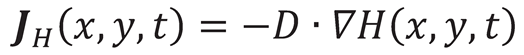
11.8. Temporal Derivative of Entropy and Maximum Temperature
Figure 11
shows the correlation between the temporal derivative of entropy (dEntropy) and
monthly maximum temperature (TmaxT_{\text{max}}Tmax), with time lags
included.
Positive correlations (0.2–0.6) dominate in Central
and Eastern Europe (Poland, Czechia, Germany, western Russia), indicating a
relationship between rapid changes in atmospheric variability and extreme
temperatures. In Greece, Turkey, and the Balkans, correlations reach up to
0.65, likely due to heatwaves and Mediterranean convective circulation.
In Western Europe (France, the UK), correlations
are weaker and more scattered—likely influenced by oceanic climate. Mountainous
and coastal areas show greater correlation variability, reflecting local
topographic and hydrological conditions.
Most common lags range from 6 to 9 months,
particularly in Central Europe. Longer lags (10–12 months) in the Baltic States
and Finland may indicate a cumulative thermal response. Shorter lags occur
mainly in coastal regions.
Figure 11.
Maximum absolute Spearman correlation at the 5% significance level.
11.9. Temporal Derivative of Entropy and Monthly Minimum Precipitation
Figure 12
presents the spatial distribution of maximum correlations between dEntropy and
monthly minimum precipitation sums.
Positive correlations (0.4–0.6) dominate in Central
and Eastern Europe (Poland, Germany, Ukraine, Belarus), suggesting that rising
climate system variability may precede periods of rainfall deficit. Western
Europe and Scandinavia show weaker correlations, possibly due to higher weather
variability and oceanic influence.
Southern Europe displays more spatially
heterogeneous correlations. Most common lag values range from 6 to 10 months,
though in parts of southern and western Europe, lags are shorter (2–5 months).
This suggests regional differences in climate sensitivity to entropy changes.
Lag analysis indicates that dEntropy could serve as
a useful early-warning indicator for seasonal drought conditions.
Figure 12.
Maximum absolute Spearman correlation at the 5% significance level.
11.10. Temporal Derivative of Entropy and Monthly Maximum Precipitation
Figure 13
illustrates the correlations between the temporal derivative of entropy and
maximum monthly precipitation totals.
The strongest positive correlations (up to 0.6)
occur in Central-Eastern Europe (Poland, Czechia, Ukraine, Romania), indicating
that dEntropy may be an effective predictor of intense rainfall episodes.
Western Europe and Scandinavia show significantly weaker correlations.
Southern Europe (Spain, Greece, Italy) exhibits
mixed relationships—both positive and negative—highlighting greater regional
complexity. High correlations in the Carpathians, Alps, and Balkans likely
reflect local orographic effects promoting convection.
Most frequent lag values fall between 6 and 10
months. In Southern Europe, shorter lags (2–5 months) dominate, possibly due to
faster atmospheric responses. The high spatial coherence of lag patterns
suggests the presence of shared circulation mechanisms.
Figure 13.
Maximum absolute Spearman correlation at the 5% significance level.
12. Entropy Relationships with Climate Indices
Informational entropy, calculated from
meteorological variables (temperature and precipitation), is increasingly
applied as an indicator for analyzing the variability and non-stationarity of
climate systems—both at regional and global scales. Particularly noteworthy is
its potential to reflect the influence of processes such as global warming
(e.g., GISTEMP index) and oceanic oscillations (e.g., ENSO – El Niño Southern
Oscillation).
Due to its sensitivity to changes in atmospheric
dynamical structure, entropy may complement classical circulation indices by
providing additional insight into the underlying mechanisms of weather systems.
The presence of strong positive correlations across Eastern and Northern Europe
suggests that entropy may serve as an indirect proxy for sea surface
temperature (SST) anomalies, while negative correlations in regions such as the
Mediterranean may indicate local hydrological anomalies or differing modes of
climate response.
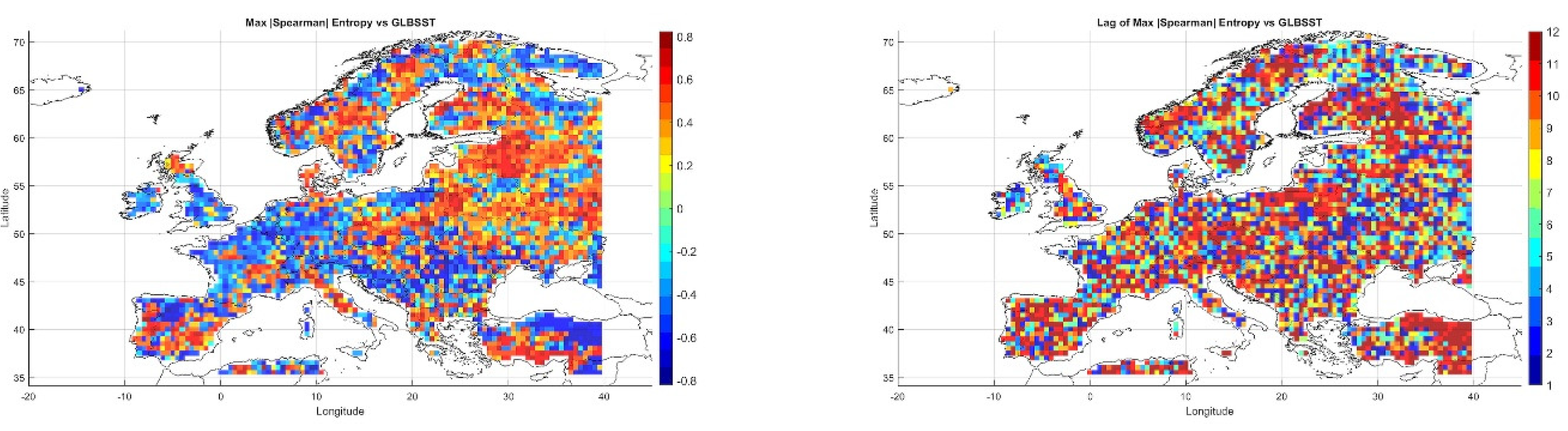
12.1. Entropy and GLBSST (GISTEMP)
Figure 14
presents the maximum absolute values of Spearman correlations between
informational entropy derived from meteorological fields and the global sea
surface temperature index GLBSST (GISTEMP), along with the corresponding time
lags.
The left panel shows that positive correlations
dominate across Central, Eastern, and Northern Europe, reaching values above
0.6 in some areas. This suggests a strong influence of global SST fluctuations
on continental climate variability.
In Southern Europe—particularly in Turkey and
northern Africa—correlations are predominantly negative, which may reflect a
distinct mechanism for GLBSST signal transmission within the Mediterranean
climate regime.
The right panel displays the spatial distribution
of time lags, which most frequently range from 9 to 12 months. This is
consistent with established mechanisms of energy transfer between ocean and
atmosphere. The homogeneity of lag times across Central and Eastern Europe
contrasts with greater variability in the south, highlighting the potential
role of local topographic conditions in modulating atmospheric response.
Figure 14.
Maximum absolute Spearman correlation at the 5% significance level.
12.2. Entropy and ENSO (NINO3.4)
Figure 15
illustrates the relationships between meteorological entropy and the ENSO index
NINO3.4, including the time lags at which the correlations are strongest. High
positive correlations (exceeding 0.6) are observed across Scandinavia, Russia,
and Central Europe, confirming the influence of ENSO on climate variability in
these regions despite their considerable distance from the tropics.
In Southern Europe—including the Mediterranean
basin, Turkey, and the Iberian Peninsula—negative correlations dominate,
suggesting an inverse ENSO effect in the warm, arid climates of the southern
continent.
The distribution of time lags shows that the
strongest correlations typically occur with lags of 8–12 months in Eastern and
Northern Europe, indicating a long-term, indirect ENSO influence via
atmospheric circulation mechanisms. In contrast, Western and Southern Europe
exhibit shorter lags (4–6 months), suggesting a faster atmospheric response.
Figure 15.
Maximum absolute Spearman correlation at the 5% significance level.
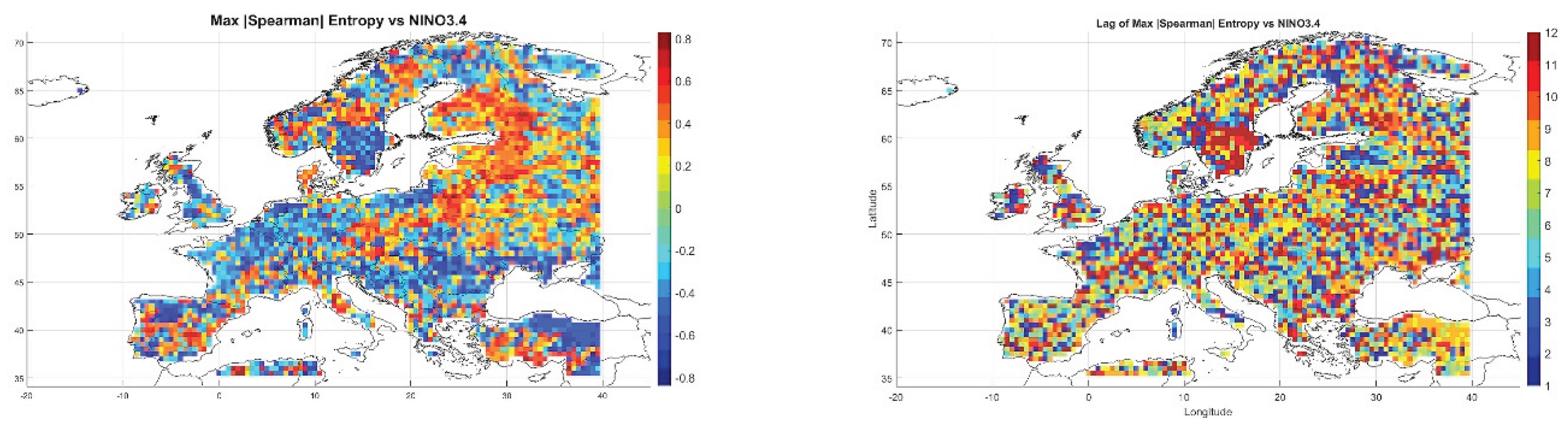
Figure 16.
Shannon entropy fluxes for temperature and precipitation across Europe.
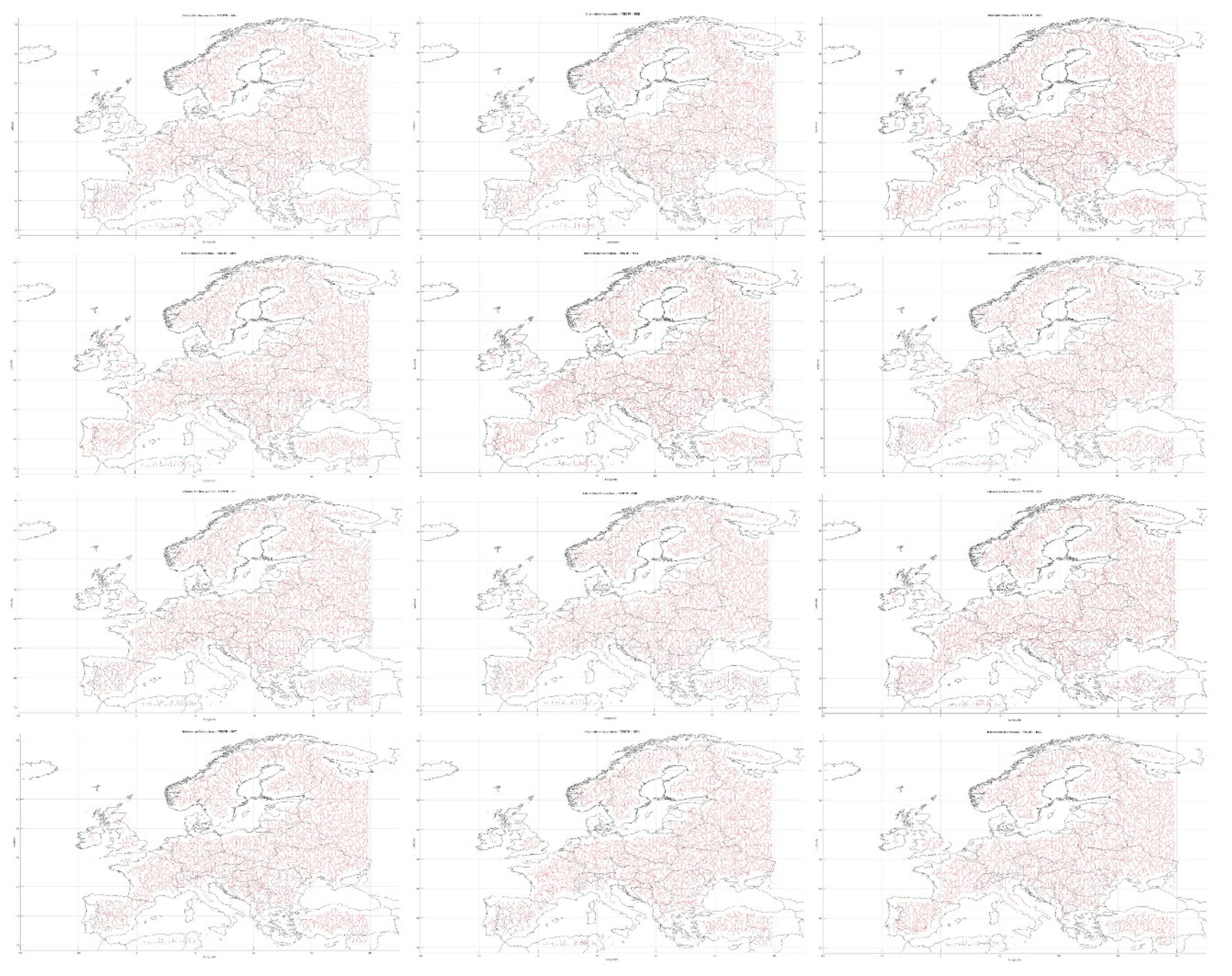
Figure 17.
Spatial–temporal components of informational entropy in the climate-scale analysis over Europe.
Figure 17.
Spatial–temporal components of informational entropy in the climate-scale analysis over Europe.
12.3. Summary
Meteorological entropy shows statistically
significant relationships with global climate indices, both in terms of
strength and spatiotemporal structure. Both GISTEMP and ENSO influence weather
variability in Europe with notable time lags, making entropy a potentially
valuable prognostic indicator—especially in early warning systems for climate
anomalies. The observed regional differences in correlation magnitude and lag
length underscore the need for local calibration and integration of entropy
into seasonal forecasting models alongside established climate indices.
13. Entropy Fluxes – Localization of Entropy Sources and Sinks
Informational entropy fluxes and their associated
sources and sinks are closely linked to prevailing atmospheric circulation
types over Europe.
Western circulation patterns (types W, SW) favor
west-to-east entropy transport, reflecting the activity of Atlantic
low-pressure systems. Anticyclonic blocking events (e.g., NE patterns,
continental regimes) are associated with the formation of “entropy holes”—areas
of reduced weather variability, particularly over Central and Eastern Europe.
Southern circulation (S, SE) is linked to local entropy sources over the
Mediterranean and Balkans, driven by convection and the influx of moist,
unstable air masses.
Elevated spatial entropy often accompanies the
passage of atmospheric fronts, especially under strong thermal gradients.
13.1. Sources and Sinks of Entropy
Regions exhibiting locally elevated entropy can be
interpreted as generators of climatic
variability, often located in dynamic transitional zones such
as:
- The Iberian Peninsula,
- The Balkans,
- Scandinavia.
In contrast, entropy sinks—areas where entropy is lower than the surrounding
environment—tend to exhibit greater atmospheric stability and are more
susceptible to external disturbances. Analyzing these structures facilitates
the identification of initiation points and propagation pathways of extreme
weather events.
13.2. Entropy Streamlines
Figure 16
presents monthly vector fields of informational entropy fluxes, calculated from
the spatial gradient of normalized entropy fields. The streamlines illustrate
the direction and relative intensity of climate information flow on a
mesoscale.
Seasonal flow patterns include:
- Winter (January–February): Dominated by organized flows from the north and northeast, especially over Scandinavia and Eastern Europe, associated with continental air masses and stable pressure systems.
- Spring (March–April): Increasing local variability and more diversified flow structures reflect the transitional nature of the season.
- Summer (July–August): Characterized by short, meandering entropy streams, indicating enhanced local turbulence. In Southern Europe, more organized westward flows appear, linked to land–ocean thermal gradients.
- Autumn (September–November): Flows begin to reorganize toward wintertime patterns. May shows intensification over the Balkans, while September highlights increased activity over Western Europe.
13.3. Sources and Convergences – Spatial Organization
Strong entropy sources and sinks—identified as
divergences and convergences of entropy streamlines—frequently appear
seasonally over Central Europe, suggesting its role as a nodal region for the transmission of climate signals.
These structures are essential for understanding the regional spread of weather
disturbances.
13.4. Links to Teleconnections and Orography
Spatial patterns of entropy fluxes demonstrate
correlations with global teleconnection indices:
- Both NAO and ENSO appear to modulate the direction and intensity of atmospheric information transport.
- Months such as March and November exhibit highly directional flows, indicating the dominance of specific circulation mechanisms.
- In other months, more chaotic flows prevail—typical of local diffusion and convective dynamics.
Topography plays
a crucial role in shaping these structures. The Alps, Carpathians, and Scandinavian Mountains
often act as barriers to the propagation of
climate information, influencing the configuration and behavior
of entropy fluxes across the continent.
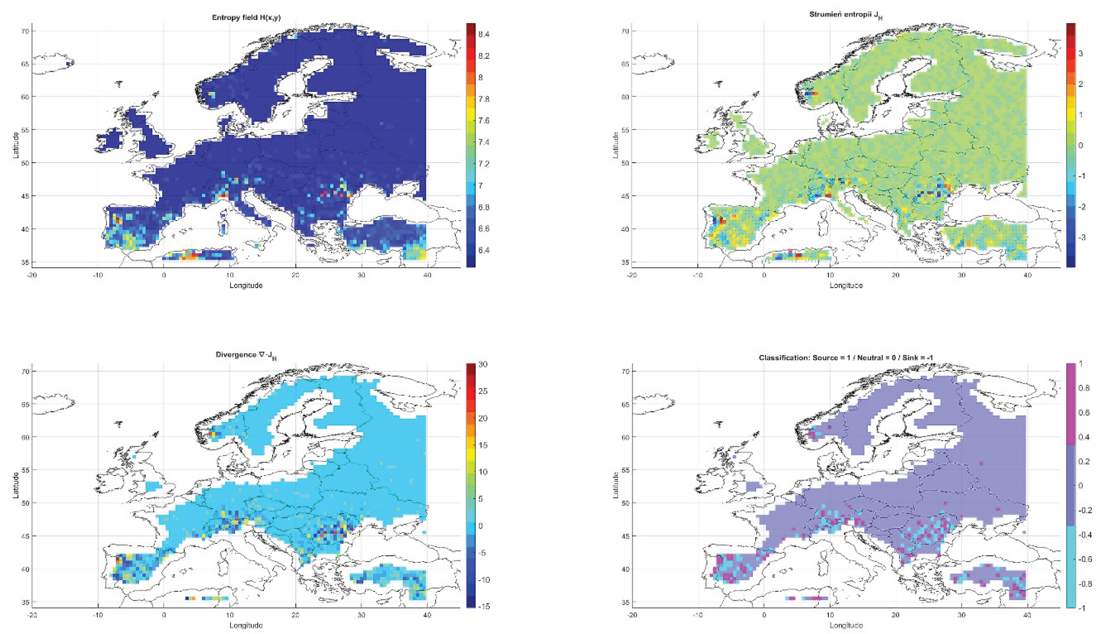
The maps in Figure
17 illustrate the key components of spatial-temporal analysis of
informational entropy at the climatic scale across Europe. The top-left panel
presents the entropy field , representing the local complexity of weather
variability as measured by Shannon entropy, calculated from the joint
distributions of temperature and precipitation. The highest entropy
values—indicating the greatest unpredictability of the weather regime—are
observed over the Mediterranean Basin and southern Balkans, suggesting
significant seasonal instability in these regions. In contrast, Northern and
Central Europe display lower , values, pointing to higher predictability of
climatic patterns, likely associated with the dominance of stable baric
systems.
The top-right panel shows the entropy flux (a vector field of information transfer), computed
as the negative gradient of the field. Areas with strong values, particularly over the Pyrenees, Alps, and
Carpathians, indicate substantial climatic information transfer between
adjacent grid cells—likely resulting from orographic influences and localized
atmospheric circulation.
The bottom-left panel depicts the divergence , identifying source regions (positive values) and
sink regions (negative values) of entropy. Notably high positive divergence
appears over southern France, Switzerland, and parts of Italy, suggesting these
as localized centers of weather variability generation. Conversely, negative
divergence values over Hungary and Romania designate these areas as entropy
sinks—absorbing external climatic signals.
To delineate neutral, source, and sink regions,
threshold values were defined based on the 5th and 95th percentiles of : the lower threshold (sink) at –3.464, and the
upper threshold (source) at 3.646. The classification shown in the bottom-right
panel assigns each grid cell to one of three categories: source (1), neutral
(0), or sink (–1). A clear dominance of the neutral state is observed,
consistent with expectations for most regions experiencing relatively
homogeneous and stable weather conditions. The notable concentration of sources
in mountainous regions emphasizes the role of topography in generating local
entropy.
The spatial analysis of the informational entropy
field reveals structured variability across Europe at the continental scale.
High entropy values cluster over southern and eastern Europe, highlighting
areas of elevated disorder and potential atmospheric instability. The entropy
field displays a clear directional structure, indicating paths of fluctuation
propagation. Entropy fluxes reveal the dominant spatial pathways of weather
information transport, strongly aligned with prevailing circulation trajectories.
A predominant west-to-east and south-to-central continental flux is observed,
reflecting the combined influence of oceanic air masses and convective activity
in southern regions. Local clustering of streamlines points to so-called
“information nodes”—regions with high potential for information exchange.
The divergence field captures zones of information
accumulation and dissipation, offering crucial insight into identifying
climatic instability sources and sinks. Areas with positive divergence are
interpreted as sources—regions initiating climate variability—while negative
divergence denotes zones that suppress instability (entropy sinks). A clear
seasonal signature of sources and sinks is also evident, which may be of
prognostic significance. Source regions often precede the emergence of
extremes, whereas sink zones may act as buffers against atmospheric
disturbances. Spatial classification also facilitates the identification of
transitional zones where local dynamics can undergo rapid shifts.
The persistent occurrence of entropy sources in
southeastern Europe may indicate a heightened climatic sensitivity to external
drivers such as ENSO. The spatial coherence of entropy fluxes and divergence
fields supports the validity of the applied mathematical formalism. This
methodological framework enables not only the visualization of the static field
of weather complexity but also the quantitative capture of the directions and
centers of atmospheric information transmission.
14. Coincidence of Extreme Weather Events with Selected Features of Informational Entropy Transport
Extreme weather phenomena—such as heatwaves,
droughts, and convective storms—demonstrate significant relationships with the
spatial and temporal characteristics of informational entropy transport.
Several key features play a critical role in this dynamic:
- Entropy sinks – regions of negative divergence in the entropy flux field ), where information streamlines converge. These areas are frequently associated with persistent anticyclonic blocks, atmospheric stagnation, and the occurrence of droughts or heatwaves. In such zones, the climate system exhibits a reduced capacity for further dynamical evolution.
- Entropy sources – areas of positive divergence (), where information fluxes diverge radially outward. These are often dynamic convective zones conducive to the generation of intense thunderstorms, convective precipitation, and hailstorms. Notable source regions include the Balkans, the Alps, the Caucasus, and the eastern Mediterranean.
- Entropy fronts – regions marked by strong spatial gradients ) and discontinuities in the entropy field. These structures typically emerge along frontal zones, at the boundaries between air masses, and over mountainous terrain. They frequently act as initiators of severe weather events, such as downpours and convective storms.
Seasonal Analysis Findings:
- In summer, localized entropy sources (e.g., over the Balkans or Mediterranean coasts) often precede the onset of storms and intense rainfall events.
- In winter, entropy sinks across Central Europe and Scandinavia correlate with cold spells and dry periods.
- In mountainous regions (such as the Alps or Carpathians), the presence of so-called “entropy holes” may favor the development of closed convective storm systems.
- Areas characterized by high entropy gradients (e.g., Scandinavia, Russia) often temporally precede episodes of winter weather extremes.
14.1. Influence of Atmospheric Circulation Patterns and Baric Systems
Western and southern circulation regimes (W, SW, S)
tend to favor the emergence of entropy sources and intensify information
fluxes. In contrast, continental high-pressure systems (NE types, anticyclones)
contribute to the closure of entropy streamlines, leading to the formation of
sinks and an elevated risk of weather stagnation.
Sudden increases in temporal entropy values may indicate seasonal transitions—such as the
shift to a wet summer or dry autumn. These inflection points often precede the
occurrence of extreme events and are consistent with trend detection
methodologies (Mann–Kendall and Pettitt tests).
14.2. Relationships with Global Indices
The occurrence of entropy sources, sinks, and
fronts is linked to broader systemic signals, including:
- ENSO (El Niño–Southern Oscillation) – particularly during El Niño phases, an increase in entropy source activity is observed over southern Europe, accompanied by intensified extreme precipitation.
- GISTEMP (Global Sea Surface Temperature Index) – correlates with entropy anomalies, especially in the Mediterranean and Eastern European regions.
14.3. Prognostic Significance
This analysis confirms that the spatial structure
of informational entropy can serve as an early indicator of forthcoming weather
extremes. Entropy values and their derivatives ) tend to lead the temporal peaks of extreme
temperatures () and precipitation ().
Locations exhibiting strong gradients, convergence
zones, and divergence structures in entropy fluxes form a predictive framework
that can be applied in:
- seasonal forecasting models,
- early warning systems,
- regional climate risk assessments.
The characteristics of entropy transport—such as
sinks, sources, discontinuities, and temporal spikes—are closely tied to the
manifestation of extreme weather events across Europe. Entropy streamlines
reflect the dynamical organization of atmospheric systems and may serve as
functional prognostic indicators. The integration of informational entropy into
climatology opens new avenues for diagnosing weather instability and for
adaptive climate risk management strategies.
15. Comparative Analysis of Correlations
15.1. Between and with Climatic Variables
Table 3
presents a comparative overview of the spatially distributed, maximum temporal
Spearman correlations between measures of entropy () and its spatial gradient with four key meteorological variables: maximum
temperature, minimum temperature, maximum precipitation, and minimum
precipitation. The Kolmogorov–Smirnov test for distribution conformity
unambiguously indicates that the correlation distributions deviate
significantly from normality (p < 10⁻¹¹).
This suggests that the information transfer between entropy and climatic
extremes is inherently nonlinear and exhibits strong spatial heterogeneity.
A comparison of the distributions of and its gradient reveals statistically significant
discrepancies, confirming that the flow of information between the two is
complex and non-uniform across space. The analysis of the number of significant
correlations (|ρ| > 0.40) shows that ENTR exhibits more
positive associations with and (exceeding 930 grid points) than with
precipitation metrics. This implies that extreme temperatures are more strongly
related to general atmospheric instability levels. In contrast, for
precipitation—especially —negative correlations dominate, indicating that
low entropy (representing more ordered conditions) is often linked to drought
scenarios.
The entropy gradient (), reflecting the spatial dynamics of variability,
shows fewer positive correlations across all variables, though the number of
negative correlations for (695) and (513) remains high. This supports the
interpretation that rapid shifts in atmospheric instability are particularly
associated with extreme precipitation events, highlighting the prognostic
utility of in this context.
The consistency in the signs of correlations
between and is relatively low—approximately 45% for all
variables—which suggests that the two metrics capture distinct mechanisms
underlying extreme events. The mean values of positive correlations for are highest for temperature variables (around
0.33) and lowest for (0.240), implying that elevated entropy values
tend to promote thermal extremes more than hydrological ones. Conversely, the
most pronounced negative correlations for are also linked to (–0.298), reinforcing the hypothesis that lower
entropy favors highly ordered, dry atmospheric states.
The entropy gradient generally shows stronger
negative correlations than positive ones, with mean values for and surpassing –0.3. This emphasizes the sensitivity
of precipitation variables to short-term dynamic fluctuations in atmospheric
structure. Differences in standard deviations across variables further indicate
that temperature correlations are more dispersed, whereas those for are more concentrated around strong negative
values.
From the perspective of information transfer, appears to better reflect long-term atmospheric
instability associated with thermal extremes. In contrast, is more useful for detecting short-term,
transitional episodes of extreme precipitation. This underscores the need to
differentiate between static () and dynamic () informational structures in extreme weather
analysis. Such differentiation is especially relevant in the design of early
warning systems, which should incorporate both the level of climatic
uncertainty (entropy) and the rate at which it changes (entropy gradient).
Ultimately, the presented data suggest that the strongest prognostic potential of ENTR and its gradient lies in their
application to thermal extremes and minimum precipitation. These insights carry
direct implications for the monitoring and forecasting of heatwaves and droughts.
Table 3.
Comparative Analysis of Maximum Temporal Spearman Correlations Between and with Meteorological Variables.
Table 3.
Comparative Analysis of Maximum Temporal Spearman Correlations Between and with Meteorological Variables.
| Criteria | ||||
| Kolmogorov-Smirnov test | stat = 0.162 | stat = 0.163 | stat = 0.164 | stat = 0.086 |
| p = 1.7e-43 | p = 8.13e-44 | p = 1.01e-44 | p = 2.71e-12 | |
| Number of correlations |ρ| > 0.40 | ||||
| positive | 930 | 931 | 741 | 333 |
| negative | 299 | 295 | 489 | 693 |
| positive | 453 | 441 | 306 | 169 |
| negative | 555 | 573 | 513 | 695 |
| Concordance of correlation sign ( vs ) | 44.68% | 44.73% | 46.03% | 46.53% |
| Positive and negative correlation statistics | ||||
| MEAN positive | 0.329 | 0.33 | 0.295 | 0.240 |
| STD positive | 0.222 | 0.221 | 0.19 | 0.171 |
| MEAN negative | -0.237 | -0.245 | -0.287 | -0.298 |
| STD negative | 0.181 | 0.183 | 0.219 | 0.205 |
| MEAN positive | 0.295 | 0.295 | 0.248 | 0.219 |
| STD positive | 0.214 | 0.214 | 0.176 | 0.162 |
| MEAN negative | -0.304 | -0.311 | -0.285 | -0.312 |
| STD negative | 0.211 | 0.215 | 0.197 | 0.205 |
15.2. Between and with Climatic Variables
Table 4 presents a comparative analysis of the maximum seasonal-spatial Spearman
correlations between entropy () and its temporal derivative () with key meteorological variables: maximum
temperature, minimum temperature, maximum precipitation, and minimum
precipitation. The Kolmogorov–Smirnov test reveals that the correlation
distributions between and with deviate significantly from normality (p < 10⁻⁴¹), highlighting the strong
nonlinearity in the relationship between information flow and extreme
temperature values. Although p-values for other variables are higher (e.g., p =
0.0383 for ), they still indicate statistically significant
differences, albeit of lower intensity.
The greatest
number of significant correlations (| ρ | > 0.40) is observed
between
and , with 1,098
positive and 966 negative correlations. This strongly confirms an informational
dependency between entropy and extreme maximum temperatures. These values are
substantially higher than those for , which yields
486 and 426 positive and negative correlations respectively. For , the number of significant correlations is more balanced and overall smaller, suggesting these
variables possess a lower informational linkage with entropy metrics.
Strikingly, the concordance in correlation signs between and is low—around 27–28% for all variables—which reinforces the idea that static entropy and its
dynamics convey different types of information about meteorological extremes.
The mean values of positive correlations for are highest for
(0.415), suggesting that elevated entropy is directly associated with heatwave occurrences. Conversely, the average of negative correlations reaches –0.401, implying that low entropy may also be reflective of mechanisms that suppress temperature extremes.
In contrast, correlations with are more symmetrical and balanced around
±0.33–0.34, indicating that entropy variability is more aligned with
transitional meteorological changes than with absolute values. Moreover, the
lower standard deviations of correlations for suggest that this derivative offers more uniform
but generally weaker informational signals than .
The implications drawn from Table 4 are important for understanding the
flow of information in the context of weather extremes. reflects accumulated atmospheric instability,
where elevated levels promote the occurrence of extreme T_max values.
Meanwhile, its temporal derivative () better captures the dynamic changes leading up to
extreme events. Particularly notable is that for precipitation variables (and ), and reach similar mean correlation values. This
suggests that the information flow associated with precipitation extremes is
not solely a function of instability level but also of its fluctuations over
time.
In summary, and are complementary informational metrics. is more effective for assessing long-term
trends—especially for extreme temperatures—while proves more useful in short-term forecasting of
meteorological changes. Such dual-perspective analysis is of significant value
for the development of early warning models and for improving predictions of
climate extremes.
Table 4.
Comparative Analysis of Maximum Seasonal-Spatial Spearman Correlations Between and with Meteorological Variables.
Table 4.
Comparative Analysis of Maximum Seasonal-Spatial Spearman Correlations Between and with Meteorological Variables.
| Criteria | ||||
| Kolmogorov-Smirnov test (Tmax) | stat = 0.151 | stat = 0.055 | stat = 0.031 | stat = 0.031 |
| p = 4.93e-42 | p = 7.1e-06 | p = 0.0383 | p = 0.0318 | |
| Number of correlations |ρ| > 0.40 | ||||
| ENTR positive | 1098 | 397 | 500 | 527 |
| ENTR negative | 966 | 520 | 518 | 545 |
| positive | 486 | 452 | 517 | 475 |
| negative | 426 | 477 | 500 | 442 |
| Concordance of correlation sign () | 27.74% | 27.72% | 28.10% | 27.15% |
| Positive and negative correlation statistics | ||||
| MEAN positive | 0.415 | 0.330 | 0.341 | 0.343 |
| STD positive | 0.117 | 0.093 | 0.097 | 0.096 |
| MEAN negative | -0.401 | -0.337 | -0.340 | -0.344 |
| STD negative | 0.115 | 0.092 | 0.092 | 0.094 |
| MEAN positive | 0.338 | 0.335 | 0.338 | 0.339 |
| STD positive | 0.088 | 0.084 | 0.086 | 0.086 |
| MEAN negative | -0.334 | -0.337 | -0.342 | -0.333 |
| STD negative | 0.087 | 0.089 | 0.089 | 0.086 |
16. Summary
The applied methodology—integrating statistics,
information theory, and the analysis of nonlinear dynamical systems—constitutes
an innovative tool for diagnosing climate instability and forecasting extreme
weather events. The use of Shannon entropy, derived from the joint distribution
of temperature and precipitation, enables a detailed assessment of seasonal and
spatial climate variability at high resolution. The model is grounded in a
well-established mathematical formalism that incorporates both the gradient and
divergence of entropy, allowing for a rigorous analysis of atmospheric
processes dispersed in time and space.
Both entropy and its spatial gradient prove to be
effective indicators of thermal and hydrological risk. In particular, the
entropy gradient enables the detection of spatial weather contrasts
and may serve as an early indicator of drought, especially in southern Europe.
The relationships between the entropy gradient and meteorological variables are
particularly strong for maximum temperature and precipitation in climatically
dynamic regions such as the Balkans, Scandinavia, and Central Europe, while
correlations with minimum variables are more heterogeneous, reflecting the
influence of local factors.
Moreover, the temporal derivative of entropy reveals nonlinear relationships between local
weather dynamics and extreme events, exhibiting high Spearman correlation
values with moderate time lags. In many regions, its spatial structure aligns
with the distribution of climatic zones, further supporting its prognostic
utility. The information entropy formalism facilitates the identification of
areas particularly susceptible to extreme weather, supports the development of
early warning systems, and enables exploration of spatial–temporal patterns not
captured by traditional statistical methods.
The inclusion of derived variables such as the
entropy flux vector () and its divergence allows for the classification of regions as
generators or suppressors of atmospheric variability, in accordance with the
principles of the Fokker–Planck equations [72].
In this framework, regions with positive divergence are interpreted as active
generators of variability, while areas with negative divergence function as
stabilizers of the climate system.
This approach, rooted in field theory and
continuous physics, can be integrated with existing meteorological and
hydrological systems. Its extension to include additional variables—such as
humidity, solar radiation, or wind—would enable a more comprehensive
representation of the climate system. Overall, the analysis of entropy and its
derivatives provides novel, high-quality tools for studying atmospheric
variability and climate adaptation, offering a coherent framework for
describing the spatiotemporal structure of weather information.
References
- Lucarini, V.; Fraedrich, K.; Lunkeit, F. Thermodynamics of Climate Change: Generalized Sensitivities. Atmos. Chem. Phys. 2010, 10, 9729–9737. [Google Scholar] [CrossRef]
- Gibbins, G.; Haigh, J.D. Entropy Production Rates of the Climate. J. Atmos. Sci. 2020, 77, 3551–3566. [Google Scholar] [CrossRef]
- Rodrigues da Silva, V. de P.; Belo Filho, A.F.; Rodrigues Almeida, R.S.; de Holanda, R.M.; da Cunha Campos, J.H.B. Shannon Information Entropy for Assessing Space-Time Variability of Rainfall and Streamflow in Semiarid Region. Sci. Total Environ. 2016, 544, 330–338. [Google Scholar] [CrossRef]
- Saha, S.; Chattopadhyay, S. Exploring of the Summer Monsoon Rainfall around the Himalayas in Time Domain through Maximization of Shannon Entropy. Theor. Appl. Climatol. 2020, 141, 133–141. [Google Scholar] [CrossRef]
- Chakrabarti, C.G.; Chakrabarty, I. Shannon Entropy: Axiomatic Characterization and Application. Int. J. Math. Math. Sci. 2005, 2005, 2847–2854. [Google Scholar] [CrossRef]
- De Michele, C.; Avanzi, F. Superstatistical Distribution of Daily Precipitation Extremes: A Worldwide Assessment. Sci. Rep. 2018, 8, 1–11. [Google Scholar] [CrossRef]
- Casquilho, J.P. On the Weighted Gini–Simpson Index: Estimating Feasible Weights Using the Optimal Point and Discussing a Link with Possibility Theory. Soft Comput. 2020, 24, 17187–17194. [Google Scholar] [CrossRef]
- Guimares Nobre, G.; Jongman, B.; Aerts, J.; Ward, P.J. The Role of Climate Variability in Extreme Floods in Europe. Environ. Res. Lett. 2017, 12. [Google Scholar] [CrossRef]
- Domínguez-Castro, F.; Reig, F.; Vicente-Serrano, S.M.; Aguilar, E.; Peña-Angulo, D.; Noguera, I.; Revuelto, J.; van der Schrier, G.; El Kenawy, A.M. A Multidecadal Assessment of Climate Indices over Europe. Sci. Data 2020, 7, 1–7. [Google Scholar] [CrossRef]
- Froyland, G.; Giannakis, D.; Lintner, B.R.; Pike, M.; Slawinska, J. Spectral Analysis of Climate Dynamics with Operator-Theoretic Approaches. Nat. Commun. 2021, 12, 1–21. [Google Scholar] [CrossRef]
- Matos, S.; Viardot, E.; Sovacool, B.K.; Geels, F.W.; Xiong, Y. Innovation and Climate Change: A Review and Introduction to the Special Issue. Technovation 2022, 117. [Google Scholar] [CrossRef]
- Twaróg, B. Application of Shannon Entropy in Assessing Changes in Precipitation Conditions and Temperature Based on Long-Term Sequences Using the Bootstrap Method. Atmosphere (Basel). 2024, 15. [Google Scholar] [CrossRef]
- Williams, J.M. Entropy Shows That Global Warming Should Cause Increased Variability in the Weather*. 2000.
- Kovács, T. How Can Contemporary Climate Research Help Understand Epidemic Dynamics? Ensemble Approach and Snapshot Attractors. J. R. Soc. Interface 2020, 17. [Google Scholar] [CrossRef] [PubMed]
- Bannon, P.R. Entropy Production and Climate Efficiency. J. Atmos. Sci. 2015, 72, 3268–3280. [Google Scholar] [CrossRef]
- Silva, A.S.A.; Menezes, R.S.C.; Rosso, O.A.; Stosic, B.; Stosic, T. Complexity Entropy-Analysis of Monthly Rainfall Time Series in Northeastern Brazil. Chaos, Solitons and Fractals 2021, 143, 110623. [Google Scholar] [CrossRef]
- Brinckmann, S.; Krähenmann, S.; Bissolli, P. High-Resolution Daily Gridded Data Sets of Air Temperature and Wind Speed for Europe. Earth Syst. Sci. Data 2016, 8, 491–516. [Google Scholar] [CrossRef]
- World Meteorological Organization Guide to Climatological Practices 2018 Edition; 2018; ISBN 9789263101006.
- Stocker, T.F.; Clarke, G.K.C.; Le Treut, H.; Lindzen, R.S.; Meleshko, V.P.; Mugara, R.K.; Palmer, T.N.; Pierrehumbert, R.T.; Sellers, P.J.; Trenberth, K.E.; et al. Physical Climate Processes and Feedbacks. Clim. Chang. 2001 Sci. Bases. Contrib. Work. Gr. I to Third Assess. Rep. Intergov. Panel Clim. Chang. 2001, 881.
- Delgado-Bonal, A.; Marshak, A.; Yang, Y.; Holdaway, D. Analyzing Changes in the Complexity of Climate in the Last Four Decades Using MERRA-2 Radiation Data. Sci. Rep. 2020, 10, 1–8. [Google Scholar] [CrossRef]
- Christensen, J.H.; Kanikicharla, K.K.; Aldrian, E.; An, S. Il; Albuquerque Cavalcanti, I.F.; de Castro, M.; Dong, W.; Goswami, P.; Hall, A.; Kanyanga, J.K.; et al. Climate Phenomena and Their Relevance for Future Regional Climate Change. Clim. Chang. 2013 Phys. Sci. Basis Work. Gr. I Contrib. to Fifth Assess. Rep. Intergov. Panel Clim. Chang. 2013, 9781107057, 1217–1308. [Google Scholar] [CrossRef]
- Kim, H.; Kim, T.; Shin, J.Y.; Heo, J.H. Improvement of Extreme Value Modeling for Extreme Rainfall Using Large-Scale Climate Modes and Considering Model Uncertainty. Water (Switzerland) 2022, 14. [Google Scholar] [CrossRef]
- Blöschl, G.; Bierkens, M.F.P.; Chambel, A.; Cudennec, C.; Destouni, G.; Fiori, A.; Kirchner, J.W.; McDonnell, J.J.; Savenije, H.H.G.; Sivapalan, M.; et al. Twenty-Three Unsolved Problems in Hydrology (UPH)–a Community Perspective. Hydrol. Sci. J. 2019, 64, 1141–1158. [Google Scholar] [CrossRef]
- Thornton, P.K.; Ericksen, P.J.; Herrero, M.; Challinor, A.J. Climate Variability and Vulnerability to Climate Change: A Review. Glob. Chang. Biol. 2014, 20, 3313–3328. [Google Scholar] [CrossRef] [PubMed]
- Tabari, H.; Willems, P. Lagged Influence of Atlantic and Pacific Climate Patterns on European Extreme Precipitation. Sci. Rep. 2018, 8, 1–11. [Google Scholar] [CrossRef]
- Cover, T.M.; Thomas, J.A. Elements of Information Theory; John Wiley & Sons, Inc, 1991; ISBN 0-471-20061-1.
- Guntu, R.K.; Agarwal, A. Investigation of Precipitation Variability and Extremes Using Information Theory. 2021; 14. [Google Scholar] [CrossRef]
- DeDeo, S.; Hawkins, R.X.D.; Klingenstein, S.; Hitchcock, T. Bootstrap Methods for the Empirical Study of Decision-Making and Information Flows in Social Systems. Entropy 2013, 15, 2246–2276. [Google Scholar] [CrossRef]
- Pitt, M.A. Increased Temperature and Entropy Production in the Earth’s Atmosphere: Effect on Wind, Precipitation, Chemical Reactions, Freezing and Melting of Ice and Electrical Activity. J. Mod. Phys. 2019, 10, 966–973. [Google Scholar] [CrossRef]
- Mills, T.C. Applied Time Series Analysis: A Practical Guide to Modeling and Forecasting; 2019; ISBN 9780128131176.
- Huser, R.; Davison, A.C. Space-Time Modelling of Extreme Events. J. R. Stat. Soc. Ser. B Stat. Methodol. 2014, 76, 439–461. [Google Scholar] [CrossRef]
- Hou, W.; Yan, P.; Feng, G.; Zuo, D. A 3D Copula Method for the Impact and Risk Assessment of Drought Disaster and an Example Application. Front. Phys. 2021, 9, 1–14. [Google Scholar] [CrossRef]
- Frees, E.W.; Valdez, E.A. Understanding Relationships Using Copulas. 1997, 1–25.
- Menne, M.J.; Durre, I.; Vose, R.S.; Gleason, B.E.; Houston, T.G. An Overview of the Global Historical Climatology Network-Daily Database. J. Atmos. Ocean. Technol. 2012, 29, 897–910. [Google Scholar] [CrossRef]
- Donat, M.G.; Alexander, L. V; Yang, H.; Durre, I.; Vose, R.; Dunn, R.J.H.; Willett, K.M.; Aguilar, E.; Brunet, M.; Caesar, J.; et al. Updated Analyses of Temperature and Precipitation Extreme Indices since the Beginning of the Twentieth Century: The HadEX2 Dataset. 2013, 118, 2098–2118. [CrossRef]
- Becker, A.; Finger, P.; Meyer-Christoffer, A.; Rudolf, B.; Schamm, K.; Schneider, U.; Ziese, M. A Description of the Global Land-Surface Precipitation Data Products of the Global Precipitation Climatology Centre with Sample Applications Including Centennial (Trend) Analysis from 1901-Present. Earth Syst. Sci. Data 2013, 5, 71–99. [Google Scholar] [CrossRef]
- Twaróg, B.S. Assessing the Polarization of Climate Phenomena Based on Long-Term Precipitation and Temperature Sequences. Sustain. 2024, 16, 31. [Google Scholar]
- Cornes, R.C.; van der Schrier, G.; van den Besselaar, E.J.M.; Jones, P.D. An Ensemble Version of the E-OBS Temperature and Precipitation Data Sets. J. Geophys. Res. Atmos. 2018, 123, 9391–9409. [Google Scholar] [CrossRef]
- Twaróg, B. Assessing the Polarization of Climate Phenomena Based on Long-Term Precipitation and Temperature Sequences; 2023.
- Drzazga-Szczȩśniak, E.A.; Kaczmarek, A.Z.; Kielak, M.; Gupta, S.; Gnyp, J.T.; Pluta, K.; Ba̧k, Z.; Szczepanik, P.; Szczȩśniak, D. Signatures of Extreme Events in Cumulative Entropic Spectrum. Entropy 2025, 27, 1–14. [Google Scholar] [CrossRef]
- Ding, D.; Zhang, M.; Pan, X.; Yang, M.; He, X. Modeling Extreme Events in Time Series Prediction. Proc. ACM SIGKDD Int. Conf. Knowl. Discov. Data Min. 2019, 1, 1114–1122. [Google Scholar] [CrossRef]
- Wenterodt, T.; Herwig, H. The Entropic Potential Concept: A New Way to Look at Energy Transfer Operations. Entropy 2014, 16, 2071–2084. [Google Scholar] [CrossRef]
- Allan, R.P.; Soden, B.J. Atmospheric Warming and the Amplification of Precipitation Extremes. Science (80-.). 2008, 321, 1481–1484. [Google Scholar] [CrossRef]
- Garbaczewski, P. Differential Entropy and Dynamics of Uncertainty. J. Stat. Phys. 2006, 123, 315–355. [Google Scholar] [CrossRef]
- Ruggeri, T. The Entropy Principle from Continuum Mechanics to Hyperbolic Systems of Balance Laws: The Modern Theory of Extended Thermodynamics. Entropy 2008, 10, 319–333. [Google Scholar] [CrossRef]
- Vavrus, S.J.; Notaro, M.; Lorenz, D.J. Interpreting Climate Model Projections of Extreme Weather Events. Weather Clim. Extrem. 2015, 10, 10–28. [Google Scholar] [CrossRef]
- Fong, S.J.; Li, G.; Dey, N.; Crespo, R.G.; Herrera-Viedma, E. Composite Monte Carlo Decision Making under High Uncertainty of Novel Coronavirus Epidemic Using Hybridized Deep Learning and Fuzzy Rule Induction. Appl. Soft Comput. J. 2020, 93. [Google Scholar] [CrossRef]
- Angélil, O.; Perkins-Kirkpatrick, S.; Alexander, L. V.; Stone, D.; Donat, M.G.; Wehner, M.; Shiogama, H.; Ciavarella, A.; Christidis, N. Comparing Regional Precipitation and Temperature Extremes in Climate Model and Reanalysis Products. Weather Clim. Extrem. 2016, 13, 35–43. [Google Scholar] [CrossRef]
- Day, W.A. Entropy and Hidden Variables in Continuum Thermodynamics. Arch. Ration. Mech. Anal. 1976, 62, 367–389. [Google Scholar] [CrossRef]
- Jaiswal, R.K.; Lohani, A.K.; Tiwari, H.L. Statistical Analysis for Change Detection and Trend Assessment in Climatological Parameters. Environ. Process. 2015, 2, 729–749. [Google Scholar] [CrossRef]
- Loehle, C. Trend Analysis of Satellite Global Temperature Data. Energy Environ. 2009, 20, 1087–1098. [Google Scholar] [CrossRef]
- Lal, P.N.; Mitchell, T.; Aldunce, P.; Auld, H.; Mechler, R.; Miyan, A.; Romano, L.E.; Zakaria, S.; Dlugolecki, A.; Masumoto, T.; et al. National Systems for Managing the Risks from Climate Extremes and Disasters; 2012; Vol. 9781107025; ISBN 9781139177245.
- Conte, L.C.; Bayer, D.M.; Bayer, F.M. Bootstrap Pettitt Test for Detecting Change Points in Hydroclimatological Data: Case Study of Itaipu Hydroelectric Plant, Brazil. Hydrol. Sci. J. 2019, 64, 1312–1326. [Google Scholar] [CrossRef]
- Fermanian, J.D. Goodness-of-Fit Tests for Copulas. J. Multivar. Anal. 2005, 95, 119–152. [Google Scholar] [CrossRef]
- Lewis, S.C.; King, A.D. Evolution of Mean, Variance and Extremes in 21st Century Temperatures. Weather Clim. Extrem. 2017, 15, 1–10. [Google Scholar] [CrossRef]
- Gurmu, S.; Dagne, G.A. Bayesian Approach to Zero-Inflated Bivariate Ordered Probit Regression Model, with an Application to Tobacco Use. J. Probab. Stat. 2012. [Google Scholar] [CrossRef]
- Ross, S.M. Introduction to Probability and Statistics for Engineers and Scientists, Fifth Edition; 2014; ISBN 9780123948113.
- Ogwang, T. Calculating a Standard Error for the Gini Coefficient: Some Further Results: Reply. Oxf. Bull. Econ. Stat. 2004, 66, 435–437. [Google Scholar] [CrossRef]
- Samson, P.; Carlen, E. Concentration of Measure Principle and Entropy-Inequalities; 2017; ISBN 9781493970049.
- Zhang, L.; Singh, V.P. Bivariate Rainfall Frequency Distributions Using Archimedean Copulas. J. Hydrol. 2007, 332, 93–109. [Google Scholar] [CrossRef]
- Management, F.R. Copulas in Financial Risk Management. Math. Financ. 2000. [Google Scholar]
- Najjari, V.; Unsal, M.G. An Application of Archimedean Copulas for Meteorological Data. Gazi Univ. J. Sci. 2012, 25, 417–424. [Google Scholar]
- Belov, D.I.; Armstrong, R.D. Distributions of the Kullback-Leibler Divergence with Applications. Br. J. Math. Stat. Psychol. 2011, 64, 291–309. [Google Scholar] [CrossRef]
- Christianto, V.; Smarandache, F. A Thousand Words: How Shannon Entropy Perspective Provides Link between Exponential Data Growth, Average Temperature of the Earth and Declining Earth Magnetic Field. Bull. Pure Appl. Sci. Geol. 2019, 38f, 225. [Google Scholar] [CrossRef]
- Silini, R.; Masoller, C. Fast and Effective Pseudo Transfer Entropy for Bivariate Data-Driven Causal Inference. Sci. Rep. 2021, 11, 1–13. [Google Scholar] [CrossRef]
- Zhang, L.; Singh, V.P. Bivariate Rainfall and Runoff Analysis Using Entropy and Copula Theories. Entropy 2012, 14, 1784–1812. [Google Scholar] [CrossRef]
- Introduction to Continuum Physics BT - Hyberbolic Conservation Laws in Continuum Physics. In; Dafermos, C.M., Ed.; Springer Berlin Heidelberg: Berlin, Heidelberg, 2005; pp. 25–49. ISBN 978-3-540-29089-6.
- Jou, D.; Lebon, G.; Mongiovì, M.S.; Peruzza, R.A. Entropy Flux in Non-Equilibrium Thermodynamics. Phys. A Stat. Mech. its Appl. 2004, 338, 445–457. [Google Scholar] [CrossRef]
- Schobeiri, M.T. Differential Operators in Continuum Mechanics BT - Tensor Analysis for Engineers and Physicists - With Application to Continuum Mechanics, Turbulence, and Einstein’s Special and General Theory of Relativity. In; Schobeiri, M.T., Ed.; Springer International Publishing: Cham, 2021; ISBN 978-3-030-35736-8. [Google Scholar]
- Kheilová, M. The Entropy Flux and the Evolution Equations for the Fluxes Including Nonlocal Terms from the Point of View of Extended Irreversible Thermodynamics. Czechoslov. J. Phys. 1999, 49, 167–176. [Google Scholar] [CrossRef]
- Ducha, F.A.; Atman, A.P.F.; Bosco de Magalhães, A.R. Information Flux in Complex Networks: Path to Stylized Facts. Phys. A Stat. Mech. its Appl. 2021, 566, 125638. [Google Scholar] [CrossRef]
- Casas, G.A.; Nobre, F.D.; Curado, E.M.F. Entropy Production and Nonlinear Fokker-Planck Equations. Phys. Rev. E - Stat. Nonlinear, Soft Matter Phys. 2012, 86. [Google Scholar] [CrossRef]
- Karmeshu Supervisor Frederick Scatena, N.N. Trend Detection in Annual Temperature & Precipitation Using the Mann Kendall Test – A Case Study to Assess Climate Change on Select States in the Northeastern United States. Mausam 2015, 66, 1–6. [Google Scholar]
- Wibig, J.; Glowicki, B. Trends of Minimum and Maximum Temperature in Poland. Clim. Res. 2002, 20, 123–133. [Google Scholar] [CrossRef]
- Pettitt, A.N. A Non-Parametric Approach to the Change-Point Problem. J. R. Stat. Soc. Ser. C (Applied Stat. 1979, 28, 126–135. [Google Scholar] [CrossRef]
- Sen, P.K. Estimates of the Regression Coefficient Based on Kendall’s Tau. J. Am. Stat. Assoc. 1968, 63, 1379–1389. [Google Scholar] [CrossRef]
- Venegas-Cordero, N.; Kundzewicz, Z.W.; Jamro, S.; Piniewski, M. Detection of Trends in Observed River Floods in Poland. J. Hydrol. Reg. Stud. 2022, 41. [Google Scholar] [CrossRef]
- Hirsch, R.M.; Slack, J.R.; Smith, R.A. Techniques of Trend Analysis for Monthly Water Quality Data. Water Resour. Res. 1982, 18, 107–121. [Google Scholar] [CrossRef]
Figure 1.
Seasonal values of Shannon entropy [bits], calculated for the final reference period 1941–2010.
Figure 1.
Seasonal values of Shannon entropy [bits], calculated for the final reference period 1941–2010.
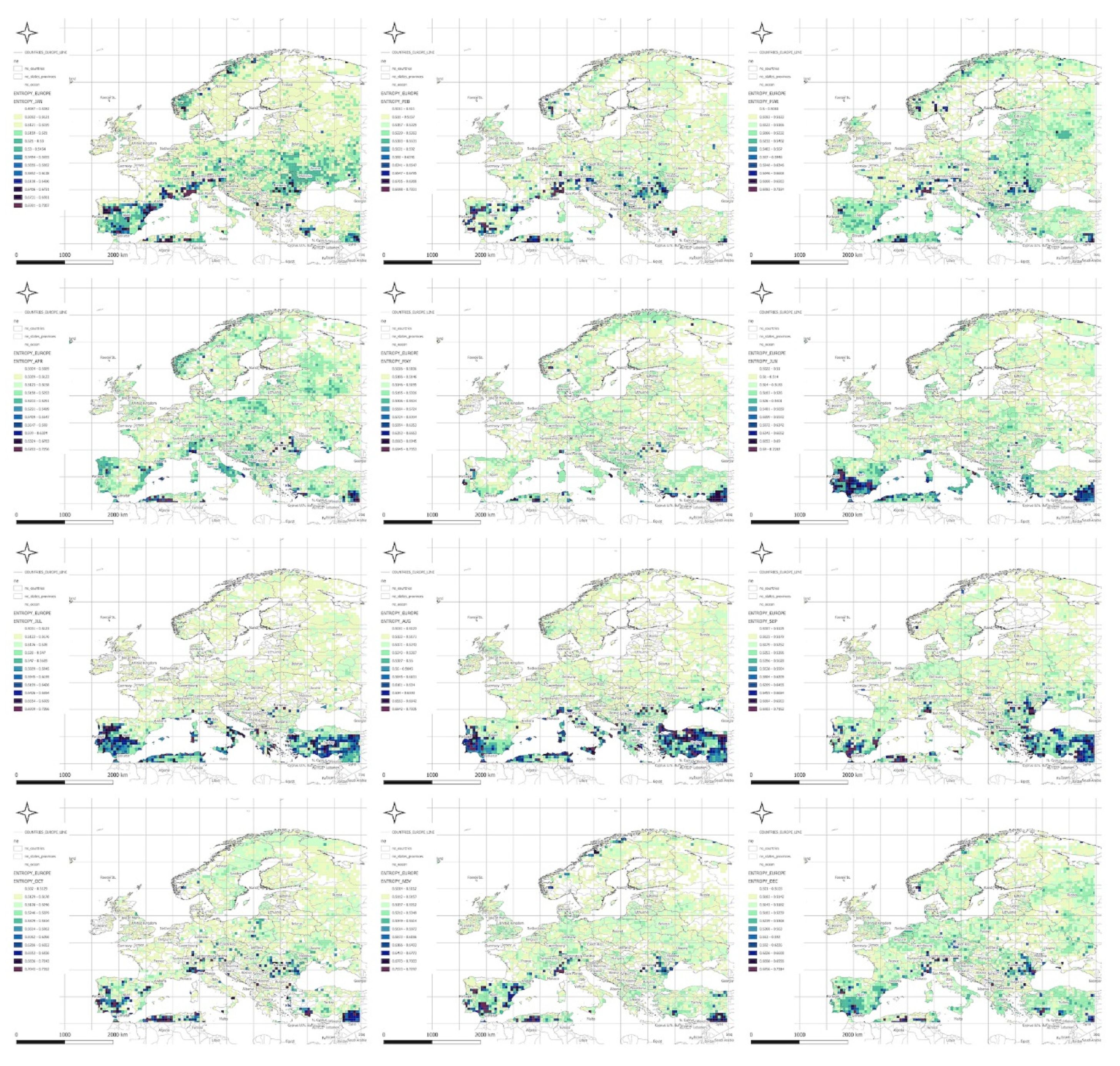
Figure 2.
Results of the Mann–Kendall Test at the 5% significance level identifying seasonal trends in Shannon entropy [bits/season].
Figure 2.
Results of the Mann–Kendall Test at the 5% significance level identifying seasonal trends in Shannon entropy [bits/season].
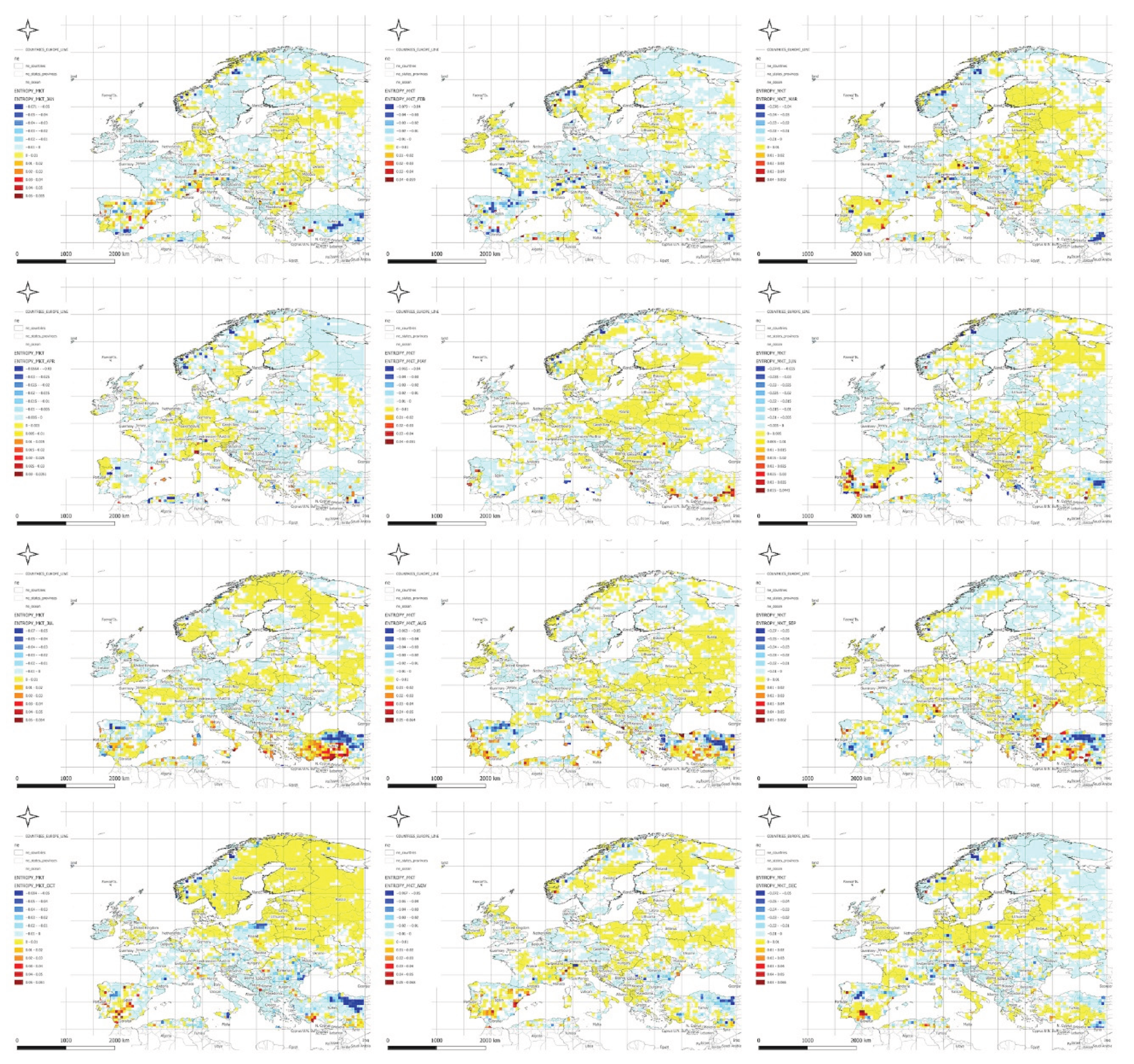
Figure 3.
Pettitt Test results at the 5% significance level indicating the years in which seasonal shifts in Shannon entropy trends occurred.
Figure 3.
Pettitt Test results at the 5% significance level indicating the years in which seasonal shifts in Shannon entropy trends occurred.
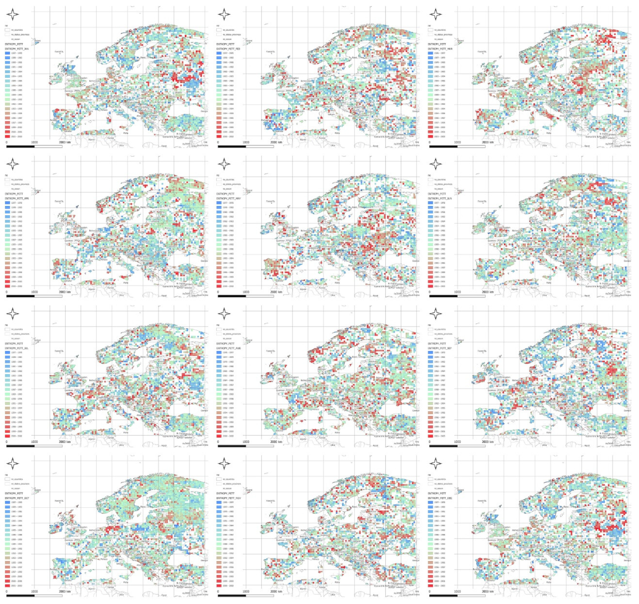
Figure 4.
Spearman correlations between entropy and meteorological parameters.
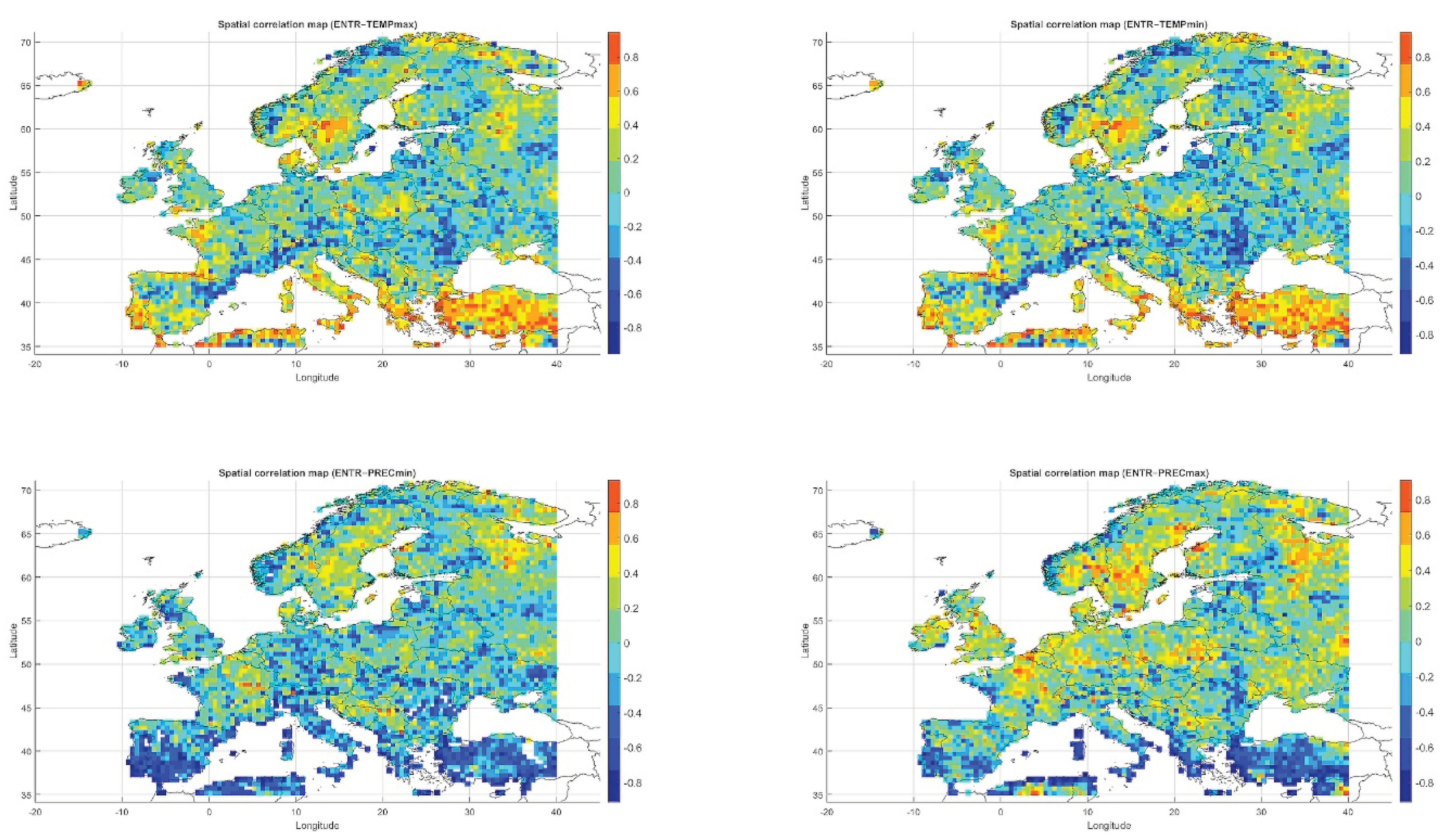
Figure 5.
Spearman correlations between entropy gradients and meteorological parameters.
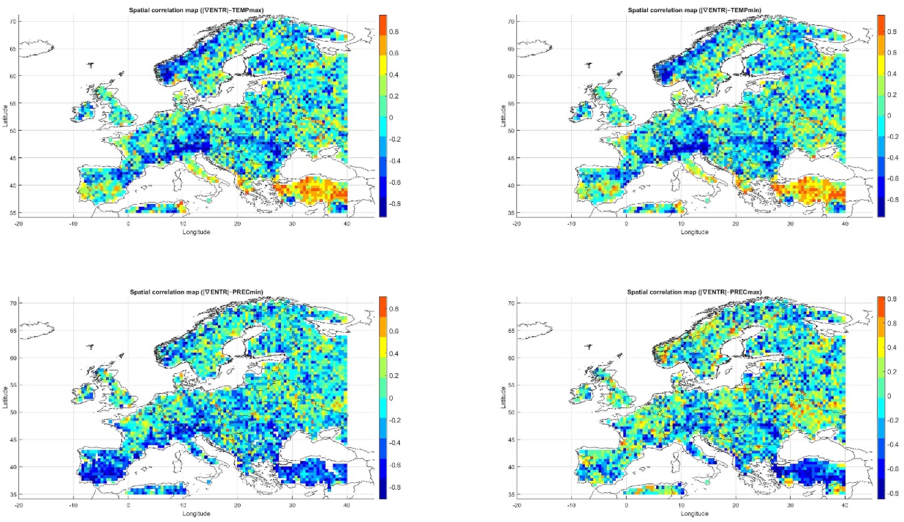
Figure 6.
Maximum absolute Spearman correlation at the 5% significance level.
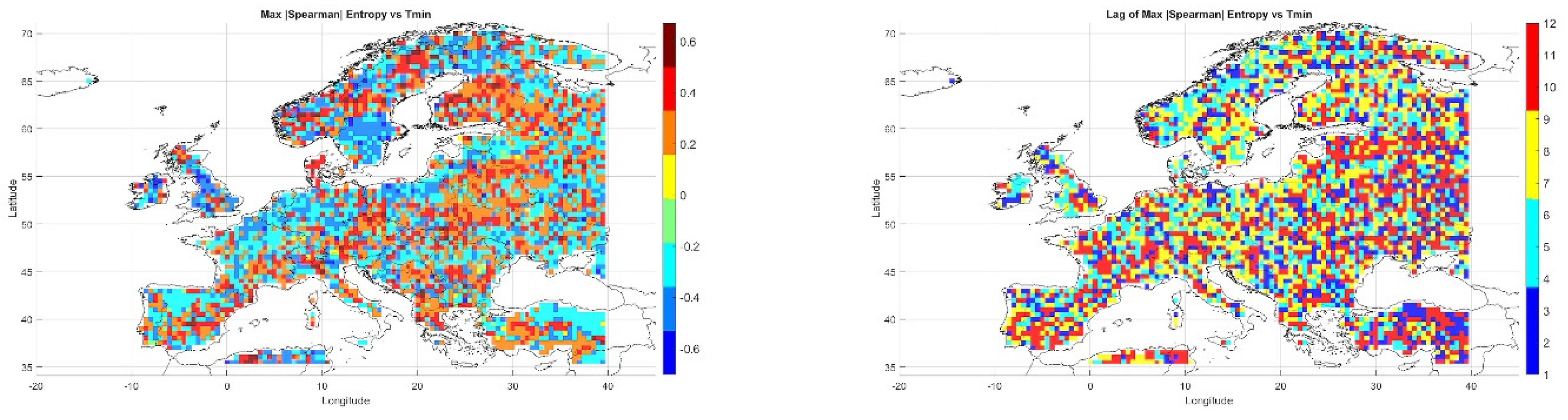
Figure 7.
Maximum absolute Spearman correlation at the 5% significance level.
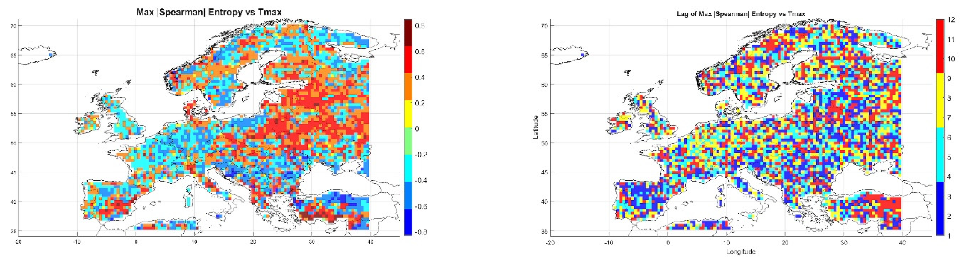
Figure 8.
Maximum absolute Spearman correlation
at the 5% significance level.
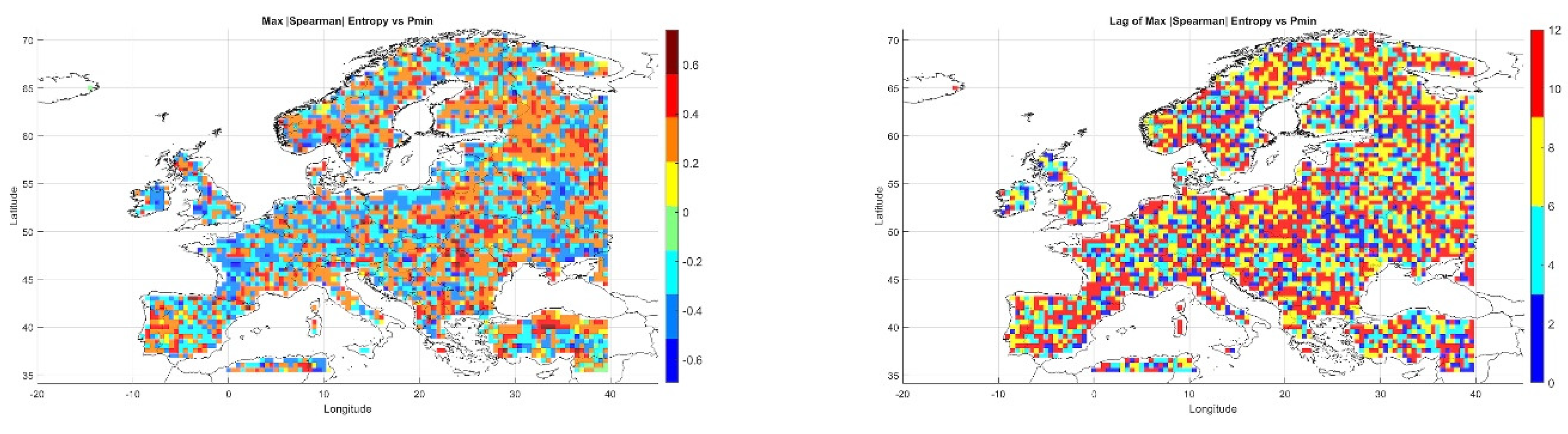
Figure 9.
Maximum absolute Spearman correlation
at the 5% significance level.
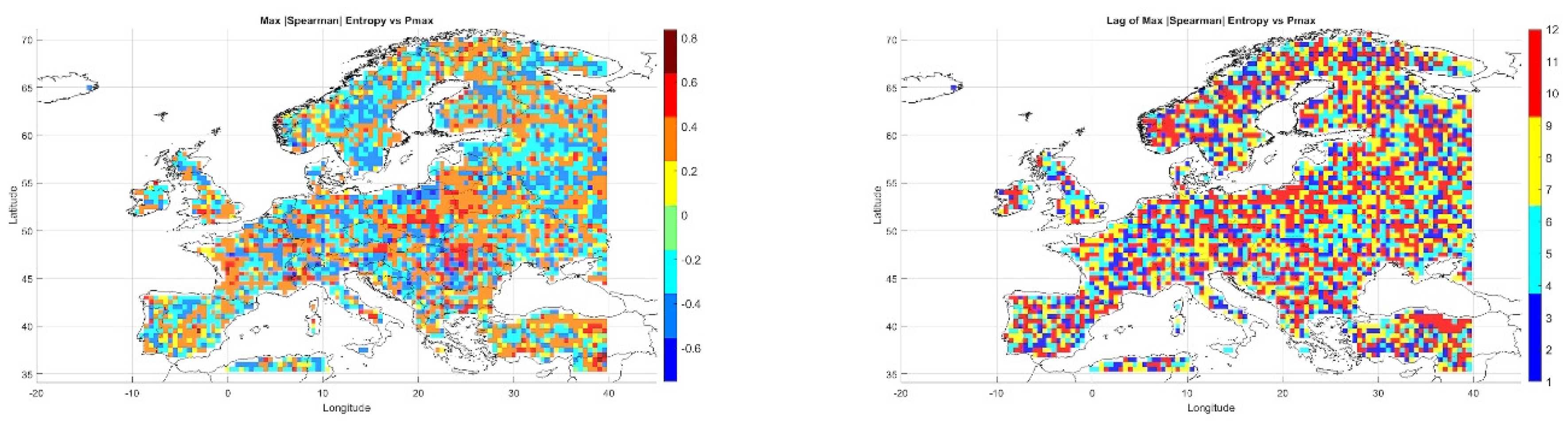
Table 2.
Analyzed forms of bivariate copula functions.
| Nazwa rozkładu | Postać matematyczna | Kendall’s τ | Eq. |
| Gaussian | where , | (8) | |
| Clayton | where | (9) | |
| Frank | where | (10) | |
| Gumbel | where | (11) |
Disclaimer/Publisher’s Note: The statements, opinions and data contained in all publications are solely those of the individual author(s) and contributor(s) and not of MDPI and/or the editor(s). MDPI and/or the editor(s) disclaim responsibility for any injury to people or property resulting from any ideas, methods, instructions or products referred to in the content. |
© 2025 by the authors. Licensee MDPI, Basel, Switzerland. This article is an open access article distributed under the terms and conditions of the Creative Commons Attribution (CC BY) license (http://creativecommons.org/licenses/by/4.0/).
Copyright: This open access article is published under a Creative Commons CC BY 4.0 license, which permit the free download, distribution, and reuse, provided that the author and preprint are cited in any reuse.


