The Dynamics of Shannon Entropy in Climate Variability Analysis: Application of the Clayton Copula for Modeling Temperature and Precipitation Uncertainty in Poland (1901–2010)

1. Introduction

Entropy, a fundamental concept in physics, plays a crucial role in analyzing climate systems. In thermodynamic terms, it describes the degree of disorder and energy dissipation, while in an informational sense (Shannon entropy), it quantifies the uncertainty and complexity of data systems, such as time series of temperature and precipitation. Recent research suggests a strong link between thermodynamic and informational entropy, enabling a new approach to analyzing climate variability. Thermodynamic entropy is essential in the operation of Earth's "heat engine" [1,2]. This system is not in thermodynamic equilibrium because temperature and pressure gradients drive atmospheric and oceanic circulation, leading to heat and moisture transfer [3,4,5]. However, the functioning of this system generates entropy through various processes, including the dissipation of kinetic energy in the atmosphere (e.g., wind friction and aerodynamic resistance), phase transitions such as water vapor condensation, ice sublimation, and snow melting, as well as heat and moisture diffusion, including heat transport between different atmospheric layers [4].

Informational entropy (Shannon entropy), on the other hand, allows for a quantitative assessment of uncertainty and randomness in climate data [6,7]. Specifically, entropy analysis of temperature and precipitation time series enables the identification of changes in their variability, which is crucial in the context of extreme weather events [8]. There is a strong relationship between thermodynamic and informational entropy—an increase in thermodynamic entropy leads to greater unpredictability and randomness in climate data. As a result, analyzing informational entropy trends in long-term time series allows for detecting changes in climate structure and assessing potential future directions of climate evolution [9,10,11]. Climate data, particularly temperature and precipitation, form the foundation for climate change analyses [xx]. These data are used across various sectors of the economy and environmental policy, including:

• Agriculture – for predicting droughts, optimizing irrigation systems, and managing agricultural production [12],
• Water management – for forecasting water resources and managing retention and flood protection [13],
• Energy sector – for assessing water availability for power plant cooling and forecasting energy demand [14],
• Urban planning – for reducing flood risk and protecting infrastructure [12],
• Medicine and public health – for predicting the impacts of heatwaves and humidity changes on human health [15].

These data enable the analysis of trends, anomalies, and the detection of extreme climate events such as intense storms, heatwaves, prolonged droughts, and floods [16]. Changes in these parameters affect Earth's energy balance and, consequently, entropy production in the climate system [3,17].

Calculating informational entropy based on temperature and precipitation distributions helps better understand climate change structures [18,19]. This is particularly important because classical statistical trend analyses often fail to capture changes in climate data variability and randomness [6,20]. Monitoring informational entropy in long-term time series allows for identifying regions at high risk of climate change, such as areas prone to increasing droughts or heavy rainfall. Analyzing informational entropy trends helps predict long-term climate changes, including the directions in which extreme events may develop. If entropy increases over time, it indicates growing climate instability and unpredictability. Such analyses can be particularly useful in forecasting future precipitation and temperature patterns, which is crucial for water resource management and urban adaptation to climate change. They also aid in assessing vulnerability to extreme meteorological events, such as more frequent heatwaves, severe storms, or thermal anomalies, and in evaluating climate change impacts on the economy, including planning adaptation strategies for the agricultural sector, forestry, and critical infrastructure [21,22].

Poland is located in a temperate transitional climate zone and is experiencing significant climate changes affecting precipitation and temperature patterns. The average temperature has been rising—between 1951 and 2021, it increased by approximately 0.28°C per decade, with winter temperatures rising even faster at 0.36°C per decade [23]. The number of hot days is increasing, particularly in the northern part of the country, leading to a higher risk of droughts [24,25,26]. At the same time, the number of frost days is decreasing, especially in northeastern Poland [27]. Precipitation changes are not uniform, but forecasts suggest an increase in the number of extreme precipitation days, mainly in eastern Poland [28,29]. Both precipitation and temperature variability exhibit characteristics of chaotic phenomena [30,31,32]. Extreme temperature and precipitation values observed in Poland may result from the interference of different circulation systems, including the interactions of air masses with distinct thermal and humidity properties [26,33]. Additionally, the increasing frequency of weather anomalies, such as intense storms or prolonged droughts, contributes to the chaotic nature of climate changes [34,35]. These findings confirm the growing variability of the climate, which can be detected through informational entropy analysis [36].

3. Bootstrap Resampling Technique

In this study, the bootstrap resampling technique was applied to estimate the distribution parameters of seasonal precipitation and temperature values. This method is preferred not only for its computational efficiency but also for its simplicity, which allows for the generation of bootstrap replications without relying on the assumption of a known underlying distribution [47]. It operates solely based on information derived from sampled data. Sequences of monthly precipitation and temperature values were generated. The number of elements in these sequences for both precipitation and temperature did not allow for a reliable assessment of Shannon entropy within the 95% confidence interval. It was assumed that the number of resamples from a 70-element sequence was 1000 [36].

To assess Shannon entropy trends, it was assumed that the 70-element sequences were generated recursively. For the estimation of monthly Shannon entropy, the calculations were based on resampled values:

$$\begin{gathered} {X^P}_i={P^{month}}_{1900+i},..,{P^{month}}_{1970+i},i=1,\dots ,40, \\ {X^T}_i={T^{month}}_{1900+i},..,{T^{month}}_{1970+i},i=1,\dots ,40 \end{gathered}$$

(1)

In this way, forty sequences of seventy elements each were arbitrarily obtained. These sequences served as a resource for 1000 bootstrap resamplings. Thus, forty 70-element sequences were bootstrapped 1000 times, and Shannon entropy was calculated within the 95% confidence interval. The above analysis was performed for all analyzed grid cells. This methodology was applied to each of the 396 grid cells in the studied area. The analysis code was developed using Matlab software.

4. Fitting the Normal and Gamma Distribution

The modeling of Shannon entropy variability in this study takes into account values for phenomena such as precipitation and temperature. A commonly used approach in entropy modeling involves extracting observation sequences from equal time periods, such as the total precipitation values for a given month. Similarly, this approach is applied to mean temperature values, assuming that the dataset is independent and identically distributed (i.i.d.). These data sets are then fitted to a probability distribution model. For monthly temperatures, the normal distribution was found to be the best fit, as confirmed by the Anderson-Darling test (ADT) [9,48]. For monthly total precipitation, the gamma distribution provided the best fit, a feature describing the randomness of precipitation sums in Poland, also validated by ADT. The parameters of these distributions were uniquely determined for each dataset, both for the normal and gamma distributions. The parameters were estimated using the Maximum Likelihood Estimation (MLE) method [49,50,51]. This methodology has been extensively studied and is considered a "user-friendly" approach.

Normal Distribution [51]:

$${f(x,\sigma ,\mu )}_S=e^{{\displaystyle \frac{-{(x-\mu )}^2}{2{\sigma }^2}}}$$

(2)

where: x$,\sigma ,\mu$ – respectively: temperature as a random variable, standard deviation, and mean value.

Gamma distribution [51]:

$${f(P/a,b)}_S={\displaystyle \frac{1}{b^a\mathsf{\Gamma }\left(a\right)}}{\mathrm{y}}^{a-1}{e}^{{\displaystyle \frac{-y}{b}}}$$

(3)

where: $y,a,b,\mathsf{\Gamma }\left(a\right)$ - respectively, precipitation as a random variable, distribution parameters, Gamma function.

5. Fitting the Copula Clayton Function

Copula functions are a statistical tool for multivariate modeling of random variable distributions. Their first applications emerged in the field of economics. They enable the combination of marginal univariate probability distributions of individual random variables into a full multivariate distribution of a multivariate random variable. The concept is not new and appeared in statistical theory over 80 years ago (Hoeffding, 1940, 1941, and Widder, 1941) [52,53,54].

Due to their ability to link marginal distributions and the increasing computational power of computers, the theory of copula functions has gained growing recognition and is increasingly applied in various fields of engineering sciences. When solving statistical or probabilistic decision-making problems, it is often necessary to determine the existence of multivariate distributions that are consistent with given marginal distributions (Nelsen, 1999; Joe, 1997; Drouet Mari & Kotz, 2001 [10]). Copula functions provide a mathematical tool to address this problem.

Typical examples from the Archimedean family include the Gumbel-Hougaard copula (both one- and two-parameter versions), the Frank copula, the Clayton copula, and the Plackett copula. Other frequently used copulas belong to the elliptical family, such as the Gaussian copula or the t-Copula [54,55,56,57].

A commonly used measure is Kendall's correlation coefficient (often denoted as τ_Kendall). Unlike Pearson’s correlation coefficient, which measures linear dependence, Kendall’s τ does not require normality of distributions and assesses the monotonic dependence between variables—it also performs well for nonlinear relationships. Kendall’s τ has a direct connection with copulas: it can be easily linked to copula parameters, allowing for the selection of an appropriate copula model for the data. It also demonstrates robustness to outliers: since it is based on ranks rather than absolute values, it is less sensitive to the influence of extreme values compared to Pearson’s correlation coefficient (Table 1).

In this study, the Clayton copula function was used to construct the joint distribution based on the marginal normal and gamma distributions [58]. The optimization of the copula parameter was performed by matching the theoretical cumulative distribution function (CDF) to the empirical CDF using the mean squared error (MSE) criterion [59,60]. The theoretical CDF was built on the marginal normal and gamma distributions with parameters estimated using the maximum likelihood estimation (MLE) method. The optimization results for the parameter θ yielded the following values for each month (Table 2).

The average values of the parameter $\theta$ illustrate the strongest relationship between precipitation and temperature during the winter months (January: 0.361, November: 0.295, December: 0.293), suggesting that these variables are more correlated in this period due to stable atmospheric conditions. The lowest values of $\theta$ occur in summer, particularly in July (0.025) and September (0.016), indicating a weaker dependence, which may result from greater variability in weather conditions, such as local storms, irregular precipitation, or heatwaves. The downward trend from January to September, followed by an increase in autumn, suggests seasonal variability in the relationship, which should be considered when modeling extreme weather events and their impact on the climate.

6. Shannon Entropy

Shannon entropy measures the uncertainty associated with predicting the value of a random variable [20,61,62]. It is calculated based on the probability distribution of the data, and its accuracy depends on the precision of this distribution. A poorly estimated distribution can lead to incorrect entropy calculations, significantly affecting the conclusions drawn about the analyzed system. The formula for Shannon entropy for a two-dimensional continuous random variable $(x,y)$ with a probability density function $f(x,y)$ is defined as [63,64,65]:

$$H_S\left(X\right)=-{\int }_{{\mathbb{R}}^2}f(x,y){\log }_{2}f\left(x,y\right)dxdy$$

(6)

Here, $f\left(x,y\right)$ is the joint PDF of the bivariate distribution derived from the copula and marginals. Marginal PDFs: the Normal and Gamma distributions, $f_X\left(x\right)$ and $f_Y\left(y\right)$. Copula density $c(u,v)$, which is derived from the Gaussian copula [62].

The formula for the joint PDF becomes:

$$f\left(x,y\right)=c(F\left(x\right),G(y\left)\right)f_X\left(x\right)f_Y\left(\mathrm{y}\right)$$

(7)

Use the definition:

$$H_S\left(X\right)=\mathrm{E}\left({\log }_{2}f\left(X,Y\right)\right)$$

(8)

to estimate the entropy as the negative mean of the log joint PDF.

In the discussion of Shannon entropy units for continuous distributions, results are typically represented in units of information, such as nats (derived from natural logarithms) or bits (using logarithms with base 2) [xx]. Despite the widespread application of this measure, it is important to acknowledge its limitations and potential pitfalls. Several key constraints of Shannon entropy deserve attention:

• Sensitivity to measurement scale: Entropy calculations are sensitive to the measurement scale. The chosen units can significantly affect the computed entropy, requiring precise definitions and appropriate scaling.
• Assumption of uniform distribution: In meteorological data, assuming a uniform distribution of all outcomes may be inaccurate, particularly since variables such as precipitation have natural constraints. This can lead to underestimation of entropy values.
• Ignoring correlations: Neglecting correlations between variables, such as temperature and precipitation, may result in overly simplified models that fail to capture the full complexity of the data.
• Data discretization: The process of categorizing data affects entropy calculations. The chosen discretization method should align with the nature of the data to ensure accurate entropy measurement.

This study focuses on computing Shannon entropy for monthly precipitation sums and average temperatures using numerical integration techniques. The sequences generated from these calculations were crucial for our further investigations into entropy variability under different climatic conditions. Anticipating potential criticisms of Shannon entropy, our approach was rigorously designed to address its known limitations. This included standardizing measurement units, selecting appropriate marginal distribution parameters, and applying a consistent discretization methodology for all analyzed data. The Anderson-Darling (AD) statistical test was employed to assess the goodness of fit between empirical and theoretical distributions, validating our data against the distributions of temperature and precipitation values. These steps ensured that our data met the strict criteria necessary for analyzing climate-related events.

7. Statistical Tests Used

To assess entropy trends for both precipitation and temperature, bootstrap resampling techniques were applied to generate sequences for Shannon entropy calculations. For each realization, the parameters of the marginal distributions of the joint distribution—constructed using the Clayton Copula—were estimated separately. The characteristics and patterns of these trends were verified using the Mann-Kendall (MK) test at a 5% significance level [66,67]. Additionally, change points in the entropy trend were identified using the Pettitt test (PCPT), also at a 5% significance level. If a change point was confirmed at this significance level, a new trend form for the subsequent sub-sequence was determined using the MK test [68,69,70]. The suitability of marginal distributions describing temperature and precipitation distributions for each analyzed value sequence was evaluated using the Anderson-Darling test (ADT), conducted at a 5% significance level.

The MK test is commonly used for detecting trends in time series and has been widely applied in scientific studies to assess trends in climate-related variables. The magnitude of the trend is estimated using the non-parametric Sen’s slope estimator, originally proposed by Sen and later extended by Hirsch [29,71]. In this study, the Shannon entropy trend was examined using this test.

Various methods can be applied to identify change points in time series. In this analysis, the non-parametric Pettitt change-point test (PCPT) was used to detect changes. PCPT, a test for abrupt changes in time series, is employed to identify a turning point where a sudden shift or "jump" occurs. This test compares the rank sums of two data subsets, divided at a threshold value, to determine whether a statistically significant change exists. Since it does not rely on the assumption of normality, it is suitable for any data distribution. The Pettitt test result is based on comparing the test statistic value with a critical value at the chosen significance level, deciding whether the null hypothesis of no sudden change can be rejected. PCPT has been widely used for detecting shifts in climatic and hydrological time series.

In this study, the presence of change points in Shannon entropy time series for monthly precipitation sums and mean monthly temperatures was examined. For sequences exhibiting a significant change point, the trend test was applied to the sub-sequences; otherwise, it was applied to the entire sequence.

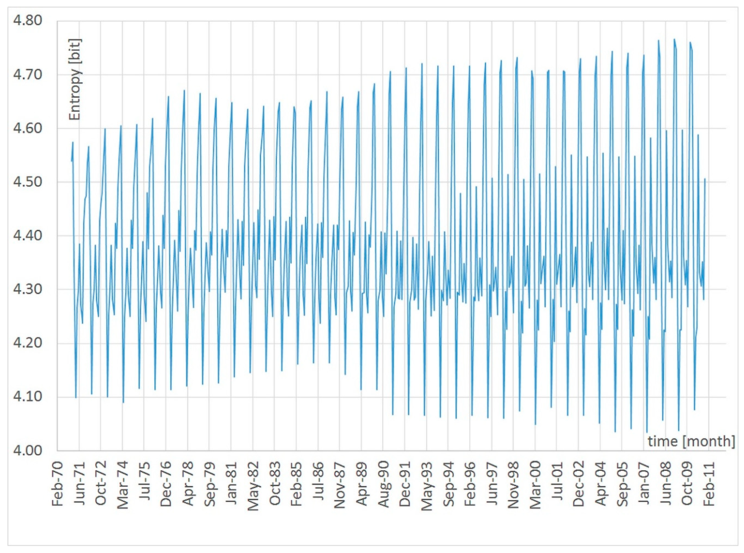
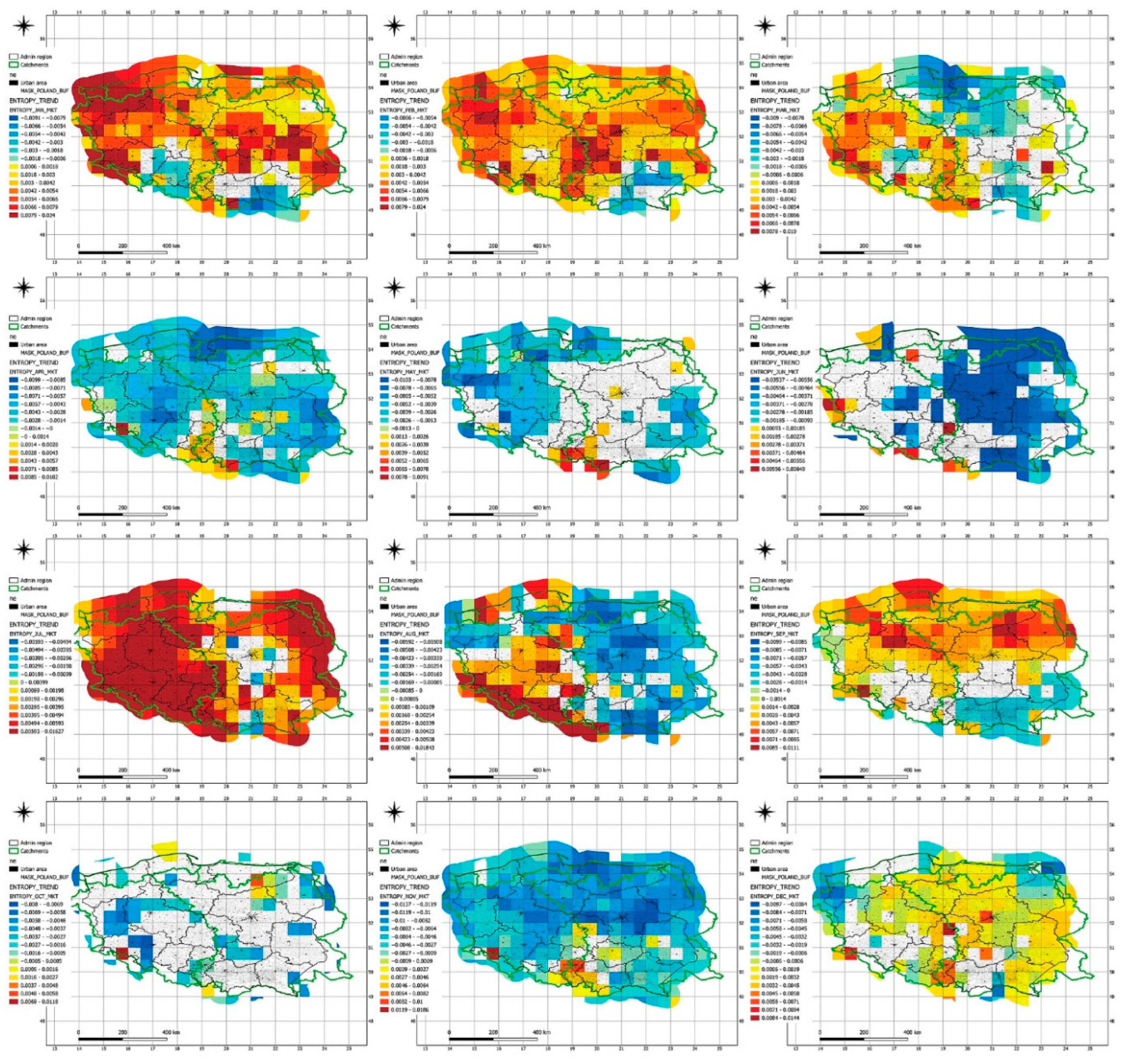
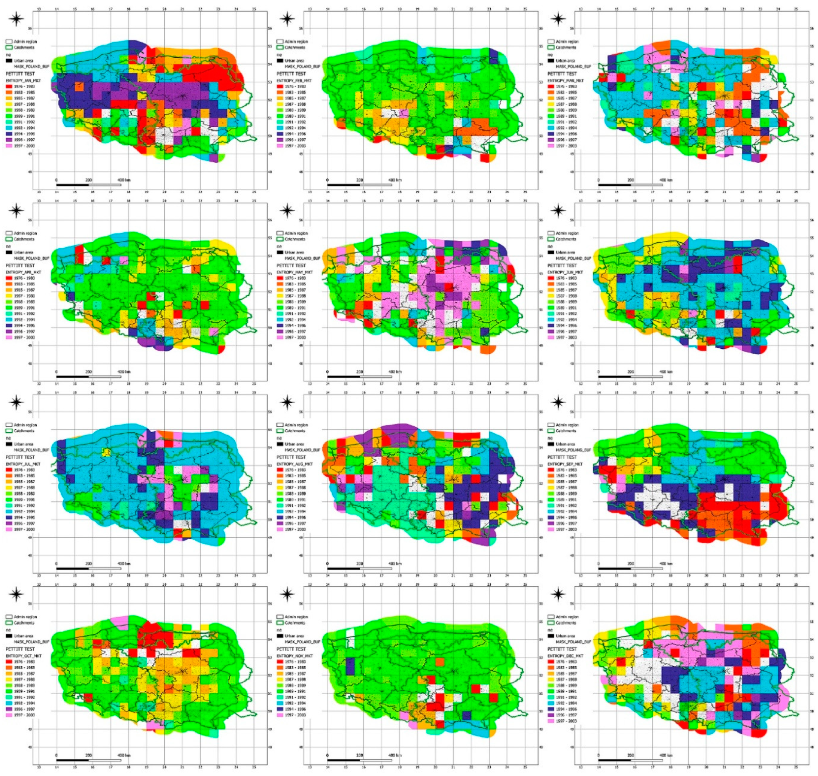
8. Analysis of Shannon's Entropy Trend Variation

The study utilized a joint distribution based on a copula, describing the combined variability of mean monthly temperature (modeled with a normal distribution) and monthly precipitation sums (modeled with a gamma distribution) [xx]. The Clayton copula was selected for entropy analysis because it best captures strong dependencies in the lower tail of the distribution, which is crucial for studying extreme events such as the simultaneous occurrence of low precipitation and high temperatures (droughts). In contrast, the Gumbel copula better describes dependencies in the upper tail of the distribution (e.g., extreme precipitation at high temperatures), which is significant in climate variability analysis, particularly when examining changes in mean values [xxx]. The Gaussian copula assumes symmetric dependencies, which do not reflect the real-world, often asymmetric relationships between precipitation and temperature [xxx]. Meanwhile, the Frank copula effectively models moderate dependencies but does not account for specific characteristics in the distribution tails, making it less precise in describing extreme weather conditions [xxx]. The fit of the empirical to theoretical cumulative distribution for the t-copula was comparable to that of the Clayton copula. However, due to the superior representation of dependencies in the lower tail, the Clayton copula was ultimately chosen for this study.

The computed Shannon entropy relates to the joint distribution of these variables, meaning it does not allow for a direct distinction between the sources of variability in temperature and precipitation separately but rather describes the overall uncertainty and disorder in their combined distribution. Interpreting Shannon entropy trends requires an approach that considers both structural changes in the climate and the dynamics of interdependencies between precipitation and temperature. An increase in entropy may result from rising unpredictability in this relationship, such as a weakening or destabilization of previously established correlations over time. This could indicate shifting climatic mechanisms, such as changes in atmospheric cycles, alterations in air circulation, or the impact of global warming on precipitation intensity within specific temperature ranges.

Assessing Shannon entropy trends for the joint distribution of precipitation and temperature is a valuable tool in climate research [88,89]. Historical data analysis helps determine the direction of changes in climate system unpredictability and provides insight into its evolution in a given region [90]. Statistical methods, such as entropy trend analysis, enhance the accuracy of climate forecasts and can support the development of adaptation strategies.

9. Results of the Analyses and Discussion

To clearly assess entropy trends for both precipitation and temperature, the bootstrap resampling method was applied to generate Shannon entropy sequences. Shannon entropy was calculated based on the joint probability distribution (Figure 1). Parameter estimation for the marginal distributions describing temperature and precipitation variability was performed using Maximum Likelihood Estimation (MLE). The significance of these trend patterns was confirmed using the Mann-Kendall (MK) test at a 5% significance level. Additionally, the Pettitt change-point test (PCPT) was applied at the same significance level to detect any shifts in entropy trends. If a change point was confirmed at the 5% level, a new trend pattern for the subsequent data subset was determined using the MK test. The adequacy of the marginal distributions for each value sequence was assessed using the Anderson-Darling test (ADT), also at a 5% significance level.

The results are presented graphically, providing a clearer and more precise visualization of the evolving entropy values and their trends.

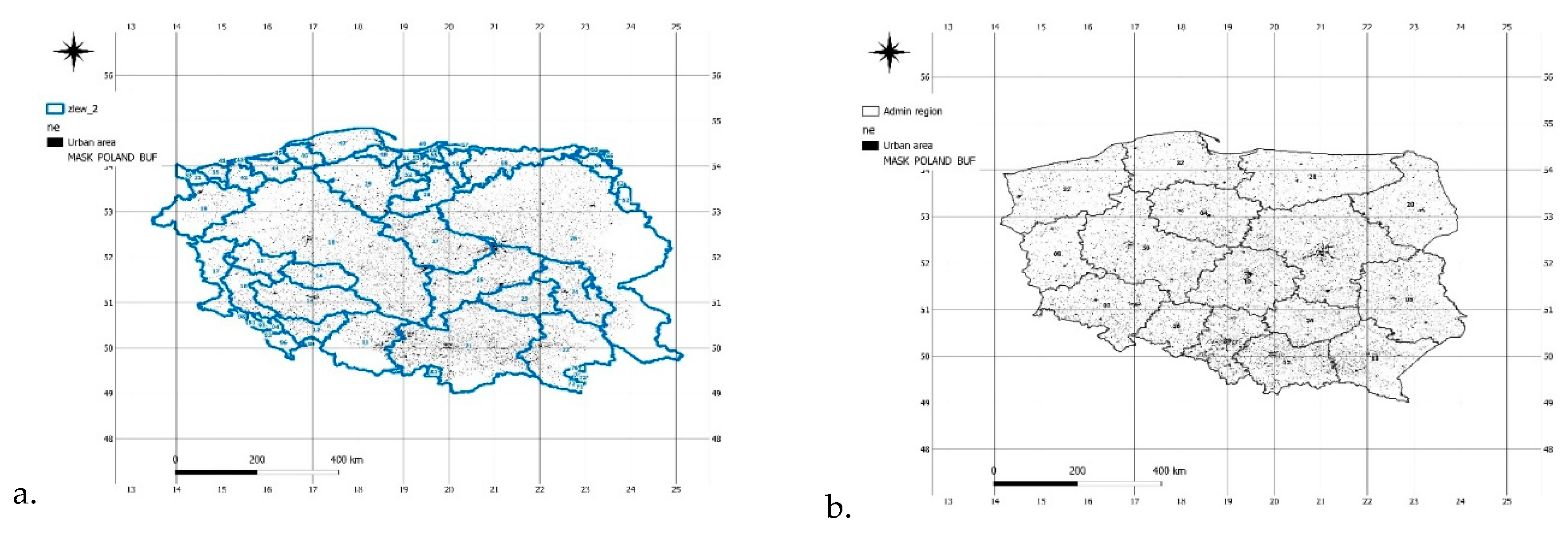
9.1. Analysis of Shannon Entropy Values in Second-Order River Basins

Shannon Entropy in the Analyzed River Basins (Figure 2a, Table 3) exhibits seasonal variability, reflecting different degrees of unpredictability in the distributions of temperature and precipitation throughout the year. The highest entropy values were recorded in the winter months, particularly in January and February, suggesting greater uncertainty in precipitation and temperature distributions during this period. Entropy values decrease in the spring and summer months, reaching their lowest levels in April and May, indicating a more predictable climate variability during this time.

The Barycz basin shows one of the lowest entropy values in April (3.726), suggesting more stable hydrological conditions in this month. Among the analyzed basins, the highest entropy in January was observed in the Bóbr River basin (5.103), indicating high uncertainty and strong fluctuations during this period. The Rega basin also has high entropy in January (5.070), which may be related to significant variability in precipitation and temperature in this region. The lowest entropy in the summer months (June–August) was recorded for the Dziwna and Barycz basins, suggesting that atmospheric conditions are more stable in these areas during summer.

In autumn, entropy gradually increases, indicating greater uncertainty during the transition period between summer and winter. The entropy values for the Nysa Kłodzka basin in August (4.498) and September (4.463) are higher than in the preceding summer months, possibly due to irregular precipitation following a drought period. The Parsęta River exhibits relatively high entropy throughout the year, suggesting significant variability in hydrometeorological conditions in this area.

The data indicate that Shannon entropy in estuarine river basins, such as the Vistula Lagoon and Martwa Wisła, is higher towards the end of the year, which may result from increased weather instability during this period. The Vistula basin, from the San to the Wieprz, maintains entropy values above 4.5 for most of the year, suggesting high unpredictability in temperature and precipitation distributions. The Shannon entropy of the Wieprz River remains at a similar level year-round, indicating a relatively even distribution of hydrological uncertainty.

Different sections of the Oder basin show variations in entropy values, reflecting regional differences in climate variability within this river basin. The entropy values suggest that the most unstable periods occur at the transition between winter and spring, as well as between autumn and winter, which aligns with typical atmospheric changes in a temperate climate.

In summary, the analysis of Shannon entropy in second-order river basins confirms that temperature and precipitation dynamics are strongly seasonally differentiated. The entropy values allow for identifying periods of greater and lesser predictability in hydrological conditions.

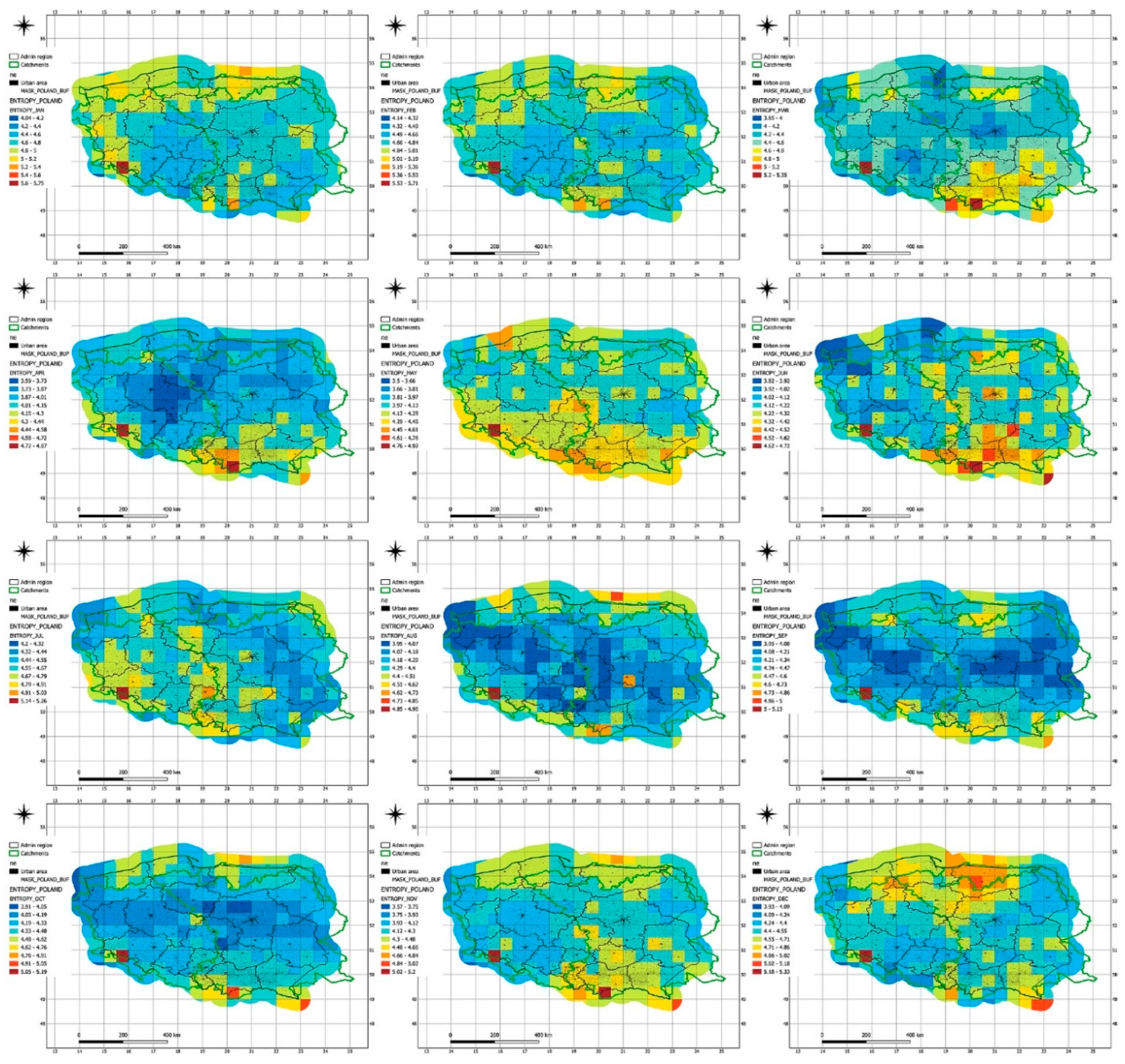
9.2. Analysis of Shannon Entropy Values in the Context of Public Administration Activities

Shannon Entropy values (Figure 2b, Table 4) indicate varying degrees of uncertainty in the distribution of temperature and precipitation across different voivodeships, which is crucial for planning adaptation measures in the context of climate change. The highest entropy values in winter months were recorded in the West Pomeranian (4.919 in January) and Warmian-Masurian (4.895 in February) voivodeships, suggesting significant variability in atmospheric conditions in these regions.

Voivodeships with high entropy values in summer months, such as Lower Silesian (4.769 in July) and Silesian (4.780 in July), may be particularly vulnerable to sudden hydrological changes, including both droughts and heavy rainfall leading to floods. Public administration in high-entropy regions should implement water management strategies, including the construction of retention reservoirs and small-scale retention systems.

Low entropy values in spring, e.g., in Greater Poland (3.753 in April) and Kuyavian-Pomeranian (3.786 in April), may indicate more stable climatic conditions but could also suggest prolonged dry periods conducive to agricultural droughts. Regional drought protection programs should consider irrigation of agricultural areas in regions with stable but low entropy in spring, such as Greater Poland and Kuyavia.

The highest climate variability occurs during transitional periods, such as in the Pomeranian Voivodeship in October (4.356), which may indicate a risk of intense rainfall and flash floods. Local governments in voivodeships with high entropy in October and November should invest in early flood warning systems and improve drainage infrastructure.

Data indicate that voivodeships with high entropy in winter, such as Warmian-Masurian (4.834 in December) and West Pomeranian (4.568 in December), may be more susceptible to temperature fluctuations and heavy snowfall. The administration in these voivodeships should focus on modernizing snow removal systems and constructing flood control reservoirs to mitigate sudden snowmelt.

The average entropy in summer months for most voivodeships ranges between 4.5 and 4.7, suggesting relatively stable but variable weather conditions, requiring flexible water management strategies. Voivodeships with high entropy in summer, such as Lublin (4.441 in July) and Świętokrzyskie (4.711 in July), may experience irregular precipitation, necessitating the construction of infrastructure to retain rainwater.

Climate change may lead to an increase in entropy in the coming decades, making it essential for public administration to implement strategies based on long-term forecasts. Local governments should integrate entropy data into crisis management systems to better respond to extreme weather events. In regions with high entropy in autumn, such as Lesser Poland (4.510 in December), increased monitoring of river and stream levels is needed to prevent the effects of heavy rainfall.

Public administration can use entropy data for spatial planning, considering areas most vulnerable to floods and droughts. Voivodeships with low entropy throughout most of the year, such as Opole (average entropy 4.2), may be less susceptible to sudden changes but still require adaptive measures.

9.3. Recommendations for Public Administration in the Context of Drought and Flood Protection and Climate Change Adaptation

Based on the analysis of Shannon entropy values (Table 4), the following recommendations for public administration regarding water resource management and climate change adaptation can be formulated. These recommendations are summarized in Table 5.

10. Trend and Seasonal Variability of Shannon Entropy in the Context of Climate Change

Shannon entropy values exhibit a general upward trend in most months, suggesting increasing climate variability over the analyzed period (1901–2010) (Table 6, Figure 3). The most significant entropy increases were observed in the summer months, particularly in July and August, where values reached their highest levels in recent decades, indicating growing instability in the distribution of temperature and precipitation.

In winter months (January, February, December), entropy also rises but at a more moderate rate, suggesting that atmospheric variability in winter is increasing more slowly than in summer. The lowest entropy values are observed in spring (April, May), indicating that weather conditions during this period are more predictable than in other months. The peak entropy values in February in recent decades (e.g., 4.747 in 2009) may indicate increasing instability in winter weather conditions, likely related to greater variability in snowfall and temperature.

The rise in entropy during summer months may result from more irregular precipitation patterns and extreme heatwaves, aligning with observed climate changes. The period from 1940 to 2010 is characterized by a noticeable increase in entropy in October and November, suggesting greater autumn weather variability, possibly due to more frequent storms and heavy rainfall.

Entropy values for summer months, particularly in July (e.g., an increase from 4.385 in 1901–1971 to 4.588 in 1940–2010), confirm the growing irregularity of seasonal precipitation, which may lead to an increased risk of droughts and flash floods. The decrease in entropy in May and June in recent decades may indicate more stabilized weather patterns during these months, although this could also be due to fewer anomalies occurring in this period.

Differences in the rate of entropy increase across months indicate that climate change does not affect all seasons equally—the highest variability occurs in summer and autumn months. In transitional months (March, September), entropy rises at a moderate pace, suggesting that while climate changes are noticeable, these periods remain relatively stable.

February exhibits some of the highest entropy values over the years, suggesting increasing variability in snowfall and temperature, leading to more unpredictable winters. Entropy values in October and November have remained high in recent decades, which may indicate an increase in extreme weather events, such as severe autumn storms.

The overall upward trend in entropy aligns with global observations of climate change, confirming the increasing instability of weather patterns. The dynamics of entropy suggest that in the future, we may expect further increases in weather unpredictability, particularly during summer and autumn, necessitating adjustments in water management strategies and climate adaptation efforts.

Analyzing the Shannon entropy values for the period 1901–2010 allows for the identification of key dynamic indicators (Table 7, Figure 4). By calculating the difference between the first period (1901–1971) and the most recent period (1940–2010), we can estimate the entropy increase over 40 years. The highest increase in entropy occurred in January (+0.221) and July (+0.203), indicating greater unpredictability in winter and summer. The largest decrease in entropy was observed in November (-0.188) and October (-0.073), suggesting greater regularity in atmospheric conditions during autumn. The average entropy growth rate per decade is highest in January (+0.055) and July (+0.051), which may indicate increasing variability in winter and summer due to climate change. Transitional months such as March, August, and September show slight increases in entropy, meaning that climate variability in these periods is lower compared to winter and summer.

Analysis of entropy trend changes in individual voivodeships (Figure 5, Table 8) indicates that the most significant changes occurred in the 1980s and 1990s, which may suggest the influence of global climate change and local environmental transformations. The earliest entropy trend changes were recorded in the Świętokrzyskie Voivodeship (September 1982) and Silesian Voivodeship (January 1983), possibly indicating early signs of climate change in these regions. The most recent trend changes occurred in the Kuyavian-Pomeranian Voivodeship (March 1996), Warmian-Masurian Voivodeship (December 1996), and Świętokrzyskie Voivodeship (May 1996, July 1996), which may suggest a later adaptation of these areas to the new climate dynamics.

Voivodeships such as Masovian, Pomeranian, and Podlaskie show a wide dispersion of trend change years, indicating a gradual and irregular impact of climate change in these regions. In contrast, voivodeships with relatively homogeneous changes within a similar period, such as Lower Silesian (1989–1992) or Lubusz (1990–1995), may have more consistent climatic and hydrological conditions affecting entropy.

Frequent changes between 1989 and 1992 in many voivodeships could be linked to the intensification of weather anomalies in Central Europe during this period, such as increased occurrences of droughts and floods. Eastern voivodeships (e.g., Lublin, Podlaskie, Subcarpathian) tend to show earlier trend changes, possibly due to their greater susceptibility to continental climate influences. Western voivodeships (e.g., West Pomeranian, Lubusz, Greater Poland) exhibit changes between 1990 and 1995, suggesting that they may have remained more climatically stable until the 1990s.

The presence of multiple trend changes in 1994–1996 in voivodeships such as Kuyavian-Pomeranian, Warmian-Masurian, and Świętokrzyskie may indicate a delayed response of these regions to climate change.

10.1. Attractor of the Mean Shannon Entropy

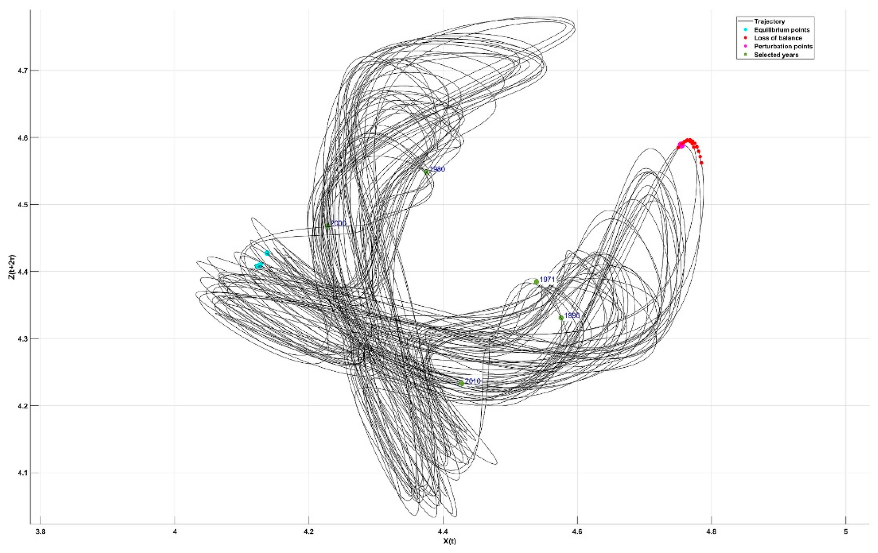
To describe the dynamics of Shannon entropy variability, a phase space analysis was performed in a three-dimensional space $\left[X\right(t),Y(t+\tau ),Z(t+2\tau \left)\right]$. The basis for constructing the plot consisted of the mean entropy values calculated for 40-year periods, separately for each of the 12 months. These values enabled the reconstruction of the system's trajectory in state space using the time delay embedding method [72,73,74].

The time delay $\tau$ was determined based on an analysis of the entropy autocorrelation function, selecting the first minimum of this function as the optimal value, $\tau$ =3 months, which indicates the lowest level of information redundancy. The calculated $\tau$ value corresponds to the optimal time shift at which the relationship between variables is strongest, allowing for the reconstruction of the system's hidden dynamic structure.

Figure 6. Attractor of the mean Shannon entropy.

Figure 6. Attractor of the mean Shannon entropy.

The attractor represents the trajectory of entropy evolution over time, highlighting areas of stable and unstable system states. Interpreting the attractor allows for the identification of equilibrium points (stable states), transitional points (unstable phases), and perturbation points (extreme changes) [75,76].

Transitional points indicate system states where small disturbances can lead to a shift into a different dynamic regime, whereas perturbation points represent moments of maximum instability, potentially linked to extreme climatic changes.

Equilibrium points, where the values of $X\left(t\right)$, $Y(t+\tau )$, and $Z(t+2\tau )$ oscillate around 4.124–4.138, 4.387–4.431, and 4.408–4.428, illustrate relatively stable climatic conditions over certain time periods. Transitional points (X=4.768, Y=4.053, Z=4.588) indicate areas where entropy undergoes irregular changes, suggesting the influence of climate anomalies. Perturbation points (X=4.755, Y=4.056, Z=4.589) mark the moments of the greatest fluctuations, where the system may transition into a new dynamic state, potentially associated with shifts in global climate trends.

For selected years, a gradual shift in entropy values can be observed, suggesting a long-term trend toward greater climatic system instability. For example, in 1971, the coordinate values (X=4.539, Y=4.099, Z=4.384) were closer to equilibrium points, indicating more predictable conditions. In the following decades (1980, 1990), entropy values shift toward greater instability, possibly linked to increasing weather anomalies.

By 2000 (X=4.707, Y=4.049, Z=4.515) and 2010 (X=4.760, Y=4.076, Z=4.588), the system approaches the characteristic values of transitional and perturbation points, suggesting an increase in irregularities in the distribution of temperature and precipitation.

Table 9. Coordinate Values of the Characteristic Points of the Attractor.

No.	Continent	X(t)	Y(t+τ)	Z(t+2τ)
1	Equilibrium Points	4.124 4.127 4.138	4.387 4.413 4.431	4.408 4.410 4.428
3	Unstable Points	4.768	4.053	4.588
4	Perturbation Points	4.755	4.056	4.589
Selected Years
5	1971	4.539	4.099	4.3845
6	1980	4.598	4.127	4.412
7	1990	4.667	4.113	4.408
8	2000	4.707	4.049	4.515
9	2010	4.760	4.076	4.588

Table 9. Coordinate Values of the Characteristic Points of the Attractor.

No.	Continent	X(t)	Y(t+τ)	Z(t+2τ)
1	Equilibrium Points	4.124 4.127 4.138	4.387 4.413 4.431	4.408 4.410 4.428
3	Unstable Points	4.768	4.053	4.588
4	Perturbation Points	4.755	4.056	4.589
Selected Years
5	1971	4.539	4.099	4.3845
6	1980	4.598	4.127	4.412
7	1990	4.667	4.113	4.408
8	2000	4.707	4.049	4.515
9	2010	4.760	4.076	4.588

The observed changes may indicate a long-term trend toward greater climate chaos, supporting the hypothesis of increasing extreme weather events. The attractor illustrates the dynamic structure of the system, revealing both periodic patterns and transitions to states of greater instability. Analyzing trajectories in phase space can aid in forecasting future climate variability by identifying transition periods and potential critical points.

The values of the attractor’s characteristic points suggest that the system exhibits features of a chaotic system, where even minor changes in initial conditions can lead to significant differences in dynamics. The data indicate that in recent decades, the climate system has gradually shifted from a stable state toward greater unpredictability. The rise in entropy in the years 2000 and 2010 compared to earlier periods may suggest a transition to a new, more unstable climate regime.

In summary, the attractor, based on the phase-space diagram and mean entropy, identifies key transition moments in climate dynamics, and its analysis can be valuable for predicting future climate changes.

11. Summary

The conducted analysis of Shannon entropy revealed significant changes in the dynamics of climate variability across different periods and spatial units. The application of the joint distribution of monthly temperatures and precipitation allowed for capturing complex dependencies between these two key meteorological parameters.

The mean entropy values, calculated for various years and months, exhibited both seasonal and long-term trends, suggesting increasing climate variability. The highest entropy values were observed in winter and summer months, indicating greater variability during these periods compared to spring and autumn. The analysis of the θ parameter for the Clayton copula confirmed that the strongest dependencies between temperature and precipitation occur in winter, while the weakest are in summer.

The phase-space diagram, constructed based on mean entropy and the time-delay embedding method, revealed the nonlinear dynamics of changes, identifying equilibrium, unstable, and perturbation points. The observed shift in entropy values over time suggests that the climate is gradually transitioning from a more predictable regime to a state of increased instability.

Equilibrium points in the analyzed attractor represented periods of stable climatic conditions, whereas perturbation points reflected periods of sudden changes. The most significant shifts in entropy dynamics occurred between 1980 and 2010, aligning with observed global warming and the intensification of extreme weather events.

The analysis of characteristic attractor points indicated that, in recent decades, the climate system has been moving toward greater instability, which could have significant implications for climate forecasting. A comparison of entropy values in selected years (1971, 1980, 1990, 2000, 2010) showed a systematic increase, suggesting growing unpredictability of atmospheric conditions. The lowest entropy values in the early decades of the 20th century indicated a more stable climate with regular weather patterns.

Current entropy values suggest a transition toward a more chaotic climate, where predicting future atmospheric conditions becomes increasingly challenging. The decrease in entropy in certain months, especially in autumn, may suggest seasonal stabilization of climatic conditions despite the overall increase in unpredictability.

The applied methodology proved effective in modeling climate dynamics, and the use of attractor analysis enabled the identification of key transition points within the system. The correlation between the years of entropy trend shifts and major periods of climate change (e.g., intensification of El Niño, increased greenhouse gas emissions, land use changes, and aerosol effects) confirms the global determinants of the analyzed processes.

References

1. Lucarini, V.; Fraedrich, K.; Lunkeit, F. ‘Thermodynamics of climate change: Generalized sensitivities’, Atmos. Chem. Phys., vol. 10, no. 20, pp. 9729–9737, 2010. [CrossRef]
2. Bannon, P.R. ‘Entropy production and climate efficiency’, J. Atmos. Sci., vol. 72, no. 8, pp. 3268–3280, 2015. [CrossRef]
3. Pitt, M.A. ‘Increased Temperature and Entropy Production in the Earth’s Atmosphere: Effect on Wind, Precipitation, Chemical Reactions, Freezing and Melting of Ice and Electrical Activity’, J. Mod. Phys., vol. 10, no. 08, pp. 966–973, 2019. [CrossRef]
4. Gibbins, G.; Haigh, J.D. ‘Entropy production rates of the climate’, J. Atmos. Sci., vol. 77, no. 10, pp. 3551–3566, 2020. [CrossRef]
5. Ghanghermeh, A.; Roshan, G.; Orosa, J.A.; Costa, Á.M. ‘Analysis and comparison of spatial-temporal entropy variability of tehran city microclimate based on climate change scenarios’, Entropy, vol. 21, no. 1, 2019. [CrossRef]
6. Atieh, M.; Rudra, R.; Gharabaghi, B. ‘Investigation of spatial and temporal variability of precipitation using an entropy theory’, ASABE 1st Clim. Chang. Symp. Adapt. Mitig., pp. 191–194, 2015. [CrossRef]
7. Organization, W.M. Guide to Climatological Practices 2018 edition, no. WMO-No. 100. 2018.
8. de P, V.; Filho, A.F.B.; Almeida, R.S.R.; de Holanda, R.M.; da Cunha Campos, J.H.B. ‘Shannon information entropy for assessing space-time variability of rainfall and streamflow in semiarid region’, Sci. Total Environ., vol. 544, pp. 330–338, 2016. [CrossRef]
9. Lewis, S.C.; King, A.D. ; Evolution of mean, variance and extremes in 21st century temperatures’, Weather Clim. Extrem., vol. 15, no. 16, pp. 1–10, 2017. 20 November. [CrossRef]
10. Pfleiderer, P.; Schleussner, C.F.; Mengel, M.; Rogelj, J. ‘Global mean temperature indicators linked to warming levels avoiding climate risks’, Environ. Res. Lett., vol. 13, no. 6, 2018. [CrossRef]
11. Miętus, M. ‘Climate of Poland 2022’, 2023, [Online]. Available: www.imgw.pl.
12. Mesbahzadeh, T.; Miglietta, M.M.; Mirakbari, M.; Sardoo, F.S.; Abdolhoseini, M. ‘Joint Modeling of Precipitation and Temperature Using Copula Theory for Current and Future Prediction under Climate Change Scenarios in Arid Lands (Case Study, Kerman Province, Iran)’, Adv. Meteorol., vol. 2019, 2019. [CrossRef]
13. Chen, L.; Guo, S. Copulas and its application in hydrology and water resources. 2019.
14. Tu, Y.X.; Kubatko, O.; Piven, V.; Sotnyk, I.; Kurbatova, T. ‘Determinants of Renewable Energy Development: Evidence from the EU Countries’, Energies, vol. 15, no. 19, pp. 1–14, 2022. [CrossRef]
15. Dankers, R.; Hiederer, R. ‘Extreme Temperatures and Precipitation in Europe: Analysis of a High-Resolution Climate Change Scenario’, JRC Sci. Tech. Reports, p. 82, 2008.
16. Rawat, A.; Kumar, D.; Khati, B.S. ‘A review on climate change impacts, models, and its consequences on different sectors: a systematic approach’, J. Water Clim. Chang., vol. 15, no. 1, pp. 104–126, 2024. [CrossRef]
17. Vinod, H.D.; López-de-Lacalle, J. ‘Maximum entropy bootstrap for time series: The meboot R package’, J. Stat. Softw., vol. 29, no. 5, pp. 1–19, 2009. [CrossRef]
18. Singh, P.; Gupta, A.; Singh, M. ‘Hydrological inferences from watershed analysis for water resource management using remote sensing and GIS techniques’, Egypt. J. Remote Sens. Sp. Sci., vol. 17, no. 2, pp. 111–121, 2014. [CrossRef]
19. Lal, P.N. et al., National systems for managing the risks from climate extremes and disasters, vol. 9781107025. 2012.
20. Guntu, R.K.; Agarwal, A. ‘Investigation of Precipitation Variability and Extremes Using Information Theory’, p. 14, 2021. [CrossRef]
21. Varbanov, P.S.; et al. ‘Efficiency measures for energy supply and use aiming for a clean circular economy’, Energy, vol. 283, p. 129035, Nov. 2023. [CrossRef]
22. Staffas, L.; Gustavsson, M.; McCormick, K. ‘Strategies and policies for the bioeconomy and bio-based economy: An analysis of official national approaches’, Sustain., vol. 5, no. 6, pp. 2751–2769, 2013. [CrossRef]
23. Marosz, M.; Miętus, M.; Biernacik, D. ‘Features of Multiannual Air Temperature Variability in Poland (1951–2021)’, Atmosphere (Basel)., vol. 14, no. 2, 2023. [CrossRef]
24. Cebulska, M.; Szczepanek, R.; Twardosz, R. Rozkład przestrzenny opadów atmosferycznych w dorzeczu górnej Wisły. 2013.
25. Cebulska, M.; Twardosz, R. ‘the Distribution of Extreme Monthly Precipitation Totals in the Polish Western Carpathians and Their Foreland Over the Year’, Prz. Geofiz., vol. 65, no. 1–2, pp. 55–68, 2020. [CrossRef]
26. Młyński, D.; Cebulska, M.; Wałȩga, A. ; Trends; variability, and seasonality of maximum annual daily precipitation in the Upper Vistula Basin, Poland’, Atmosphere (Basel)., vol. 9, no. 8, pp. 1–14, 2018. [CrossRef]
27. Ziernicka-Wojtaszek, A.; Zawora, T. ‘Thermal regions in light of contemporary climate change in Poland’, Polish J. Environ. Stud., vol. 20, no. 6, pp. 1627–1632, 2011.
28. Struzewska, J.; Kaminski, J.W.; Jefimow, M. ‘Changes in Temperature and Precipitation Trends in Selected Polish Cities Based on the Results of Regional EURO-CORDEX Climate Models in the 2030–2050 Horizon’, Appl. Sci., vol. 14, no. 1, 2024. [CrossRef]
29. Venegas-Cordero, N.; Kundzewicz, Z.W.; Jamro, S.; Piniewski, M. ‘Detection of trends in observed river floods in Poland’, J. Hydrol. Reg. Stud., vol. 41, no. 21, 2022. 20 December. [CrossRef]
30. Christensen, J.H.; et al. ‘Climate phenomena and their relevance for future regional climate change’, Clim. Chang. 2013 Phys. Sci. Basis Work. Gr. I Contrib. to Fifth Assess. Rep. Intergov. Panel Clim. Chang., vol. 9781107057, pp. 1217–1308, 2013. [CrossRef]
31. Easterling, D.R.; Kunkel, K.E.; Wehner, M.F.; Sun, L. ‘Detection and attribution of climate extremes in the observed record’, Weather Clim. Extrem., vol. 11, pp. 17–27, 2016. [CrossRef]
32. Zhang, Y.; Zhao, Y.; Shen, X.; Zhang, J., ‘A comprehensive wind speed prediction system based on Monte Carlo and artificial intelligence algorithms’. Appl. Energy 2021, 305, 117815. [CrossRef]
33. Młyński, D.; Wałȩga, A.; Petroselli, A.; Tauro, F.; Cebulska, M. ‘Estimating maximum daily precipitation in the Upper Vistula Basin, Poland’, Atmosphere (Basel)., vol. 10, no. 2, 2019. [CrossRef]
34. Stocker, T.F.; et al. ‘Physical Climate Processes and Feedbacks’, Clim. Chang. 2001 Sci. Bases. Contrib. Work. Gr. I to Third Assess. Rep. Intergov. Panel Clim. Chang., p. 881, 2001.
35. Beillouin, D.; Schauberger, B.; Bastos, A.; Ciais, P.; Makowski, D. ‘Impact of extreme weather conditions on European crop production in 2018: Random forest - Yield anomalies’, Philos. Trans. R. Soc. B Biol. Sci., vol. 375, no. 1810, 2020. [CrossRef]
36. Twaróg, B. ‘Application of Shannon Entropy in Assessing Changes in Precipitation Conditions and Temperature Based on Long-Term Sequences Using the Bootstrap Method’, Atmosphere (Basel)., vol. 15, no. 8, 2024. [CrossRef]
37. Menne, M.J.; Durre, I.; Vose, R.S.; Gleason, B.E.; Houston, T.G. ‘An overview of the global historical climatology network-daily database’, J. Atmos. Ocean. Technol., vol. 29, no. 7, pp. 897–910, 2012. [CrossRef]
38. Donat, M.G.; et al. ‘Updated analyses of temperature and precipitation extreme indices since the beginning of the twentieth century : The HadEX2 dataset’, vol. 118, pp. 2098–2118, 2013. [CrossRef]
39. Becker, A.; et al. ‘A description of the global land-surface precipitation data products of the Global Precipitation Climatology Centre with sample applications including centennial (trend) analysis from 1901-present’, Earth Syst. Sci. Data, vol. 5, no. 1, pp. 71–99, 2013. [CrossRef]
40. B. Twaróg, ‘Assessing the Polarization of Climate Phenomena Based on Long-Term Precipitation and Temperature Sequences’, 2023. doi: 2023040380. [CrossRef]
41. Allan, R.P.; Soden, B.J. ‘Atmospheric warming and the amplification of precipitation extremes’, Science (80-. )., vol. 321, no. 5895, pp. 1481–1484, 2008. [CrossRef]
42. Labriet, M.; Espegren, K.; Giannakidis, G.; Gallachóir, B.Ó., Aligning the Energy Transition with the Sustainable Development Goals: Key Insights from Energy System Modelling, vol. 101. 2024.
43. Asadieh, B.; Krakauer, N.Y. ‘Global trends in extreme precipitation: Climate models versus observations’, Hydrol. Earth Syst. Sci., vol. 19, no. 2, pp. 877–891, 2015. [CrossRef]
44. Hao, Z. ‘Application of Entropy Theory In Hydrologic Analysis And Simulation’, PENGARUH Pengguna. PASTA LABU KUNING (Cucurbita Moschata) UNTUK SUBSTITUSI TEPUNG TERIGU DENGAN PENAMBAHAN TEPUNG ANGKAK DALAM PEMBUATAN MIE KERING, vol. 15, no. 1, pp. 165–175, 2016, [Online]. Available: https://core.ac.uk/download/pdf/196255896.pdf.
45. Hou, W.; Yan, P.; Feng, G.; Zuo, D. ‘A 3D Copula Method for the Impact and Risk Assessment of Drought Disaster and an Example Application’, Front. Phys., vol. 9, no. April, pp. 1–14, 2021. [CrossRef]
46. DeDeo, S.; Hawkins, R.X.D.; Klingenstein, S.; Hitchcock, T. ‘Bootstrap methods for the empirical study of decision-making and information flows in social systems’, Entropy, vol. 15, no. 6, pp. 2246–2276, 2013. [CrossRef]
47. Ng, J.L.; Aziz, S.A.; Huang, Y.F.; Mirzaei, M.; Wayayok, A.; Rowshon, M.K. ‘Uncertainty analysis of rainfall depth duration frequency curves using the bootstrap resampling technique’, J. Earth Syst. Sci., vol. 128, no. 5, pp. 1–15, 2019. [CrossRef]
48. C. De Michele and F. Avanzi, ‘Superstatistical distribution of daily precipitation extremes: A worldwide assessment’, Sci. Rep., vol. 8, no. 1, pp. 1–11, 2018. [CrossRef]
49. Huser, R.; Davison, A.C. ‘Space-time modelling of extreme events’, J. R. Stat. Soc. Ser. B Stat. Methodol., vol. 76, no. 2, pp. 439–461, 2014. [CrossRef]
50. Gurmu, S.; Dagne, G.A. ‘Bayesian approach to zero-inflated bivariate ordered probit regression model, with an application to tobacco use’, J. Probab. Stat., 2012. [CrossRef]
51. Ross, S.M. Introduction to Probability and Statistics for Engineers and Scientists, Fifth Edition. 2014.
52. Ogwang, T. ‘Calculating a standard error for the Gini coefficient: Some further results: Reply’, Oxf. Bull. Econ. Stat., vol. 66, no. 3, pp. 435–437, 2004. [CrossRef]
53. Samson, P.; Carlen, E. Concentration of measure principle and entropy-inequalities. 2017.
54. Zhang, L.; Singh, V.P. ‘Bivariate rainfall frequency distributions using Archimedean copulas’, J. Hydrol., vol. 332, no. 1–2, pp. 93–109, 2007. [CrossRef]
55. Najjari, V.; Unsal, M.G. ‘An Application of Archimedean Copulas for Meteorological Data’, Gazi Univ. J. Sci., vol. 25, no. 2, pp. 417–424, 2012.
56. Frees, E.W.; Valdez, E.A. ‘Understanding Relationships Using Copulas’, no. 1996, pp. 1–25, 1997.
57. Management, F.R. ‘Copulas in Financial Risk Management’, Math. Financ., no. August, 2000.
58. Cherubini, U.; Luciano, E. Copula methods in finance. 2004.
59. Panchenko, V. ‘Goodness-of-fit test for copulas’, Phys. A Stat. Mech. its Appl., vol. 355, no. 1, pp. 176–182, 2005. [CrossRef]
60. Fermanian, J.D. ‘Goodness-of-fit tests for copulas’, J. Multivar. Anal., vol. 95, no. 1, pp. 119–152, 2005. [CrossRef]
61. Christianto, V.; Smarandache, F. ‘A Thousand Words: How Shannon Entropy Perspective Provides Link between Exponential Data Growth, Average Temperature of the Earth and Declining Earth Magnetic Field’, Bull. Pure Appl. Sci. Geol., vol. 38f, no. 2, p. 225, 2019. [CrossRef]
62. Chakrabarti, C.G.; Chakrabarty, I. ‘Shannon entropy: Axiomatic characterization and application’, Int. J. Math. Math. Sci., vol. 2005, no. 17, pp. 2847–2854, 2005. [CrossRef]
63. Cover, T.M.; Thomas, J.A. Elements of Information Theory. John Wiley & Sons, Inc, 1991.
64. Silini, R.; Masoller, C. ‘Fast and effective pseudo transfer entropy for bivariate data-driven causal inference’, Sci. Rep., vol. 11, no. 1, pp. 1–13, 2021. [CrossRef]
65. Zhang, L.; Singh, V.P. ‘Bivariate rainfall and runoff analysis using entropy and copula theories’, Entropy, vol. 14, no. 9, pp. 1784–1812, 2012. [CrossRef]
66. N. N. Karmeshu Supervisor Frederick Scatena, ‘Trend Detection in Annual Temperature & Precipitation using the Mann Kendall Test – A Case Study to Assess Climate Change on Select States in the Northeastern United States’, Mausam, vol. 66, no. 1, pp. 1–6, 2015, [Online]. Available: http://repository.upenn.edu/mes_capstones/47.
67. Wibig, J.; Glowicki, B. ‘Trends of minimum and maximum temperature in Poland’, Clim. Res., vol. 20, no. 2, pp. 123–133, 2002. [CrossRef]
68. Conte, L.C.; Bayer, D.M.; Bayer, F.M. ‘Bootstrap Pettitt test for detecting change points in hydroclimatological data: case study of Itaipu Hydroelectric Plant, Brazil’, Hydrol. Sci. J., vol. 64, no. 11, pp. 1312–1326, 2019. [CrossRef]
69. Pettitt, A.N. ‘A Non-Parametric Approach to the Change-Point Problem’, J. R. Stat. Soc. Ser. C (Applied Stat., vol. 28, no. 2, pp. 126–135, Apr. 1979. [CrossRef]
70. Jaiswal, R.K.; Lohani, A.K.; Tiwari, H.L. ‘Statistical Analysis for Change Detection and Trend Assessment in Climatological Parameters’, Environ. Process., vol. 2, no. 4, pp. 729–749, 2015. [CrossRef]
71. Hirsch, R.M.; Slack, J.R.; Smith, R.A. ‘Techniques of trend analysis for monthly water quality data’, Water Resour. Res., vol. 18, no. 1, pp. 107–121, Feb. 1982. [CrossRef]
72. Froyland, G.; Giannakis, D.; Lintner, B.R.; Pike, M.; Slawinska, J. ‘Spectral analysis of climate dynamics with operator-theoretic approaches’, Nat. Commun., vol. 12, no. 1, pp. 1–21, 2021. [CrossRef]
73. Essex, C.; Lookman, T.; Nerenberg, M.A.H. ‘The climate attractor over short timescales’, Nature, vol. 326, no. 6108, pp. 64–66, 1987. [CrossRef]
74. Kovács, T. ‘How can contemporary climate research help understand epidemic dynamics? Ensemble approach and snapshot attractors’, J. R. Soc. Interface, vol. 17, no. 173, 2020. [CrossRef]
75. Bhattacharya, K. ; The climate attractor’; Sci, P.I.A.S.-E.P.; vol.; no.; pp., 1993. [CrossRef]
76. Brunetti, M.; Ragon, C. ‘Attractors and bifurcation diagrams in complex climate models’, Phys. Rev. E, vol. 107, no. 5, 2023. [CrossRef]
Figure 1. Seasonal Shannon entropy values calculated for the most recent period (1941–2010).
Preprints 151180 g001
Figure 2. Location of river basins (a) and public administration units (b) with corresponding codes.
Preprints 151180 g002
Figure 3. Average Shannon Entropy in the Years 1971–2010.
Preprints 151180 g003
Figure 4. Results of the Mann-Kendall test determined at a 5% significance level identifying seasonal trends in Shannon entropy [bits/season].
Preprints 151180 g004
Figure 5. Results of the Pettitt test at a 5% significance level identifying the years in which changes in seasonal trends of Shannon entropy occurred.
Preprints 151180 g005